Abstract
We present an extension of the polarization coherence theorem (PCT) for the case in which two qubits play similarly important roles. The standard version of the PCT: , involves three measures, visibility , distinguishability , and the degree of polarization , all of which refer to a single qubit, regardless of its physical realization. This is also the case with the inequality that is implied by the PCT: , which was originally derived in an attempt to quantify Bohr’s complementarity principle. We show that all of these constraints hold true, no matter how the involved qubits are physically realized, either as quantum or else as classical objects.
1. Introduction
Somewhat prematurely perhaps, a “second quantum revolution” has already been announced while research institutions and industry are still making efforts to develop the most basic quantum technologies. Alongside other platforms, optics and photonics are expected to play a key role in this enterprise. Technological breakthroughs are widely expected, based on quantum properties, such as coherent state superposition, entanglement, and measurement collapses. It is rather ironic that precisely these three quantum properties have been identified and highlighted by the optics community [1]. Indeed, despite the widely held identification of those properties as unique quantum ones, they are also exhibited by classical electromagnetic fields [2]. For example, a polarized plane wave can be represented as the coherent superposition of, say, horizontally and vertically polarized states [3]. Entanglement may involve two or more degrees of freedom (DOFs) that are carried along by classical light beams [4,5,6,7,8,9,10]. A polarizing beam-splitter supplemented with a couple of birefringent plates constitute the perfect analog of a Stern–Gerlach device, giving rise to measurement collapses [11]. Even so, it is not our purpose here to deny the possibility of so-called quantum advantages. Rather, we aim at sharpening the identification of those resources that could allow us to implement these advantages. It might be the case that what is really exploited by some quantum algorithms, quantum protocols, and the like, are, in fact, features that are not exclusively tied to quantum phenomena, but to the linear algebraic formalism used to describe these phenomena. In that case, we could widen the spectrum of physical tools that can be employed for reaching quantum advantage. This spectrum might include physical phenomena and techniques that belong to the classical domain. The sweet spot of such a development would be a stage at which one has reached quantum advantage without quantum fragility. Thus, it seems worthwhile to strip off the quantum or classical rhetoric that often accompany our mathematical description of physical phenomena and so lay bare the essential features that we are actually addressing.
In this work, we address a feature that is often referred to as a genuinely quantum one: wave-particle duality. We will show that what recent, quantitative approaches to wave-particle duality in fact engage, is a couple of DOFs. As long as the latter can be ascribed to both quantum and classical entities, we can exhibit wave-particle duality by employing quantum as well as classical tools, e.g., photons and classical light beams. Perhaps considering a mechanical-electrical analogy helps to clarify what we mean. The said analogy applies when an electric circuit and a mechanical system obey one and the same differential equation, e.g., the one established in the textbook cases of an LCR circuit and a damped mass-spring system. It is merely a matter of convention to say that one system simulates the other, so that, by means of, say, the time-varying position, one can simulate the time-varying electric current. Suppose next that we design some protocol based on properties of the common differential equation governing the two cases, the mechanical and the electrical. We could implement this protocol either with mechanical or else with electrical tools. Even if we mentally link the differential equation with an electric current and we imagine this current as being made of electrons, i.e., spin-1/2, charged particles that interact with an ion-lattice, nothing of this is captured by the differential equation. Something similar could happen with those features that exclusively stem from the linear algebraic structure that is used to describe some quantum phenomena. Even though we keep connecting said algebraic structure with the phenomena it is supposed to describe, the linear structure by itself could also describe phenomena of a very different nature, as it occurs with the mechanical-electrical analogy.
We will illustrate the foregoing state of affairs by first addressing two recent results about wave-particle duality, which have been couched in quantum-mechanical terms. As we shall see, the very same results hold true when dealing with classical light beams. That is, what we really engage here is a linear algebraic structure that underlies the description of some properties that are shared by quantum and classical light. Each of the two examples incorporates a feature hitherto neglected when dealing with wave-particle duality. In one case, the new feature is polarization [12] and in the other case it is entanglement [13]. We should stress that polarization can be defined whenever we deal with a two-state system and entanglement whenever we deal with two vector spaces, out of which we construct their tensor product space. The corresponding physical realization might be optical or something else.
We will also present an extension of the polarization coherence theorem (PCT) [14,15,16] to the case in which two qubits are engaged. Besides having a richer structure than the standard PCT, this extension makes clear how many DOFs are actually engaged in one and the other case. Here, again, it is the linear algebraic structure what really matters, irrespective of its physical realization, which could be classical or quantal.
2. Two-Slit Interference and Wave-Particle Duality
A general setting for addressing wave-particle duality is the Young-type, two-beam interference setup that is schematically shown in Figure 1. In the quantum context, this setup is used to exhibit wave and particle properties. In accordance with our mental pictures of particles and waves, we put which-path information in the set of particle-like features, and the capability to produce an interferometric pattern in the set of wave-like features. One set is complementary to the other, which means that, the more features from one set show up, the less show up from the other. Complementarity can be quantified by defining measurable quantities that we naturally associate with the features we have in mind. In the Young-type scenario, there are three locations, , , and , at which we perform measurements (see Figure 1). These measurements essentially consist on some counting process (of particles, excitations, etc.). In the quantum case, counting leads to probability measurements, and in the classical case it leads to intensity measurements. To fix ideas, let us suppose that we measure intensities at the three locations. We get and at the two fixed locations, and , respectively, and at the variable location on the detection screen.
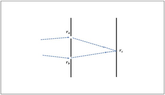
Figure 1.
Young setup.
Now, the two-path alternative of the Young-type setup can be mathematically encoded in terms of a two-dimensional vector space, whose members can be written as . Here, and in what follows, the Dirac notation does not necessarily refer to a quantum description. Indeed, may denote just the a-beam, a concept that can be both quantal (photon beam) and classical (optical beam). For the sake of concreteness, let us take as describing the path-state at the two-slit screen. When this state propagates towards the detection screen, the coefficients and change, being modified by propagation factors. The path difference is what matters, i.e., the difference between and . Denoting this difference by z, the intensity at point on the detection screen will be of the form
with , , and with the angular brackets denoting statistical averages. By changing the detection point , viz. z, we display the periodic variation of that makes up the interferometric pattern. We interpret this pattern in terms of constructive and destructive interferences, something attributable to a wave-like phenomenon. The difference between and gives us instead which-path information, something that is attributable to a particle-like phenomenon.
In order to give quantitative support to our interpretations, we first construct a matrix M with elements , where . We next define distinguishability () and visibility () by
We see that and are defined in terms of a single DOF that is associated with a two-level system, a qubit in modern parlance. This DOF can be physically realized in different ways: as a two-path alternative, as a horizontally/vertically polarized state, as a spin up/down state, as a two-state Josephson junction, etc. The hermitian matrix M gives rise to a third definition, which is similar to those of and . We define the “degree of polarization” in terms of the eigenvalues of M, as follows:
Using , we obtain
From , it follows the constraint , which was established by different authors (see [14,17,18,19] and references therein), before the PCT was known [14]. Equation (5), in turn, has also been subsequently derived in different ways and with various backgrounds. Correspondingly, people have used different definitions of distinguishability. For instance, it has been occasionally called “predictability” by other authors [17]. The meaning we give here to should be unambiguous, as it is fixed by its mathematical definition. The same holds for and . In what follows, we focus on two recent results that involve these quantities.
2.1. Complementarity and the Degree of Polarization
In Ref. [12], the PCT is obtained by considering two orthogonal polarization modes , where represents a single-photon polarized along direction x, and similarly . A general, possibly mixed polarization state can be represented by a density matrix . This matrix can be written in the form [20]
where , with being a coherent superposition, while contributes an incoherent mixture, and . Given a density matrix , one can always decompose it as in Equation (6), by setting . In Ref. [12], the PCT is re-derived and written in the form
The derivation rests upon the following results [12]:
with . There is a lot of physical background in Ref. [12], of which we want to point out only some few features. Two-point Stokes parameters are introduced as , with . Here, is the identity matrix, are the Pauli matrices and are the positive and negative frequency parts of the electric field operator. The quantum parameters are analogs of classical, two-point Stokes parameters [21,22,23,24]. The one-point, standard Stokes parameters are given by . “Intensity distinguishability” is similarly defined to in Equation (2), substituting and , whereas visibility is expanded from being a single quantity to four similarly defined quantities, one for each Stokes parameter. Such an approach unveils several hitherto neglected aspects of complementarity. However, the point that we want to make here is that none of these aspects effectively enter Equation (7). Indeed, let us write of Equation (6) explicitly:
By applying the definitions of , and given in (2) and (3), with , we obtain , and , as above. That is, despite all of the physical background that is supposed to underlie Equation (7), what this relationship is actually capable of exhibiting is no more than what is contained in (5). The exclusive dependence of on and , cf. (11), makes clear that reference to four different locations in , and is rather decorative than informative. Hence, experiments testing or exploiting (5) and (7) can be equally performed with polarized single photons, polarized optical beams, or any two-state system of whatever sort. Our interpretation, in terms of wave-particle duality, largely depends on our mental pictures rather than on bare facts. If, for instance, our two-state system is a polarized state, as assumed in [12,25], there are no actual paths involved and the Young-type setup only exists in the abstract polarization space. To talk about “wave” and “particle” in this case seems to be out of place and, yet, such a parlance would be no less supported by experimental facts than the corresponding one that is associated to a Young, double-slit experiment conducted with electrons or photons.
2.2. Entanglement as an Additional Coherence
Let us now turn to another recent result in which wave-particle duality has been couched in quantum terms [13]. In this case, entanglement is addressed by writing (5) in the form [13,26]
where denotes Wooters’ concurrence [27]. Equation (12) and (5) are the same, because for pure, bipartite states, it holds [28,29,30,31]. According to [13], Equation (12) is the correct single-particle duality restriction. This is so, because the restriction allows that both and simultaneously increase or decrease, it being possible that . In this last case, we should say that we have neither a particle nor a wave, while we can be dealing with, say, a detectable photon in a state for which . Thus, concurrence provides what is missing in the constraint . Ref. [13] reports the experimental tests of (12) that were conducted with single photons prepared in the state
with . The vectors represent propagation modes and polarization modes, with and . Here, and stand for horizontally and vertically polarized photons, respectively. Seven points lying on an octant of the -sphere defined by (12) were experimentally tested. , and were expressed in terms of the control parameters and , as [13]
The experimental results reported in [13] closely match the theoretical expressions, including the case , for which “traditional duality” is “turned off” [13]. In such a case, the single-particle coherence that remains active is entanglement. These results were interpreted as a manifestation of self-interference and self-entanglement of individual quantum particles [13].
Here again, what has been effectively tested is something that can be equally well ascribed to quantum and to classical phenomena. Indeed, the state in (13) belongs to a tensorial product space that can be physically realized in different ways. is a two-qubit, pure state, alternatively represented by the density matrix . By tracing over one DOF, one obtains a , reduced density matrix that describes the other DOF. The reduced density matrix corresponds to a mixed state, unless the two-qubit state is a factorable one.
Hence, we can define and . Using the definitions of and that are given in (2), first with and then with , we obtain
It should be clear that has the same value for and , because the two-qubit state can be brought to the Schmidt form , with and orthonormal basis vectors in their respective subspaces. The eigenvalues of the reduced density matrices, and , are, thus, , and is defined in terms of these eigenvalues. On replacing (17) in , we recover the expression for given in (14).
We can readily see that the two pairs, , and , , satisfy Equation (12). Hence, (12) could be tested with , as it was with . Of course, the experimental setup should be changed. Moreover, the experiments that were reported in [13] could have been conducted with optical light beams. The conclusions would have been the same, because all that enters in the tested results is the interplay between two DOFs, mathematically encoded in two qubits. It would be a matter of pure convention to say that one type of experiment simulates the other. Laying bare what we are really addressing also has practical advantages. Because the relationships (5) and (12) are, in fact, the same, by testing one of them, we are also testing the other. However, in order to obtain experimentally, it is common practice to perform two-qubit tomography. This generally requires sixteen measurements and maximum-likelihood parameter estimation [32]. To obtain instead, one measures the four Stokes parameters that belong to any of the two single-qubit, reduced density matrices or . Of course, two-qubit tomography provides more information than single-qubit tomography, but this information is not captured by the single parameter any more than it is captured by .
We have seen in the two cases above that they essentially address some DOFs, which can be carried by classical or quantum entities. Each of the two cases effectively deals with only one qubit. In what follows, we will discuss similar approaches that deal with two qubits.
3. Two Qubits in Alternating Roles
As we already said, before the PCT was established, the constraint had been derived by several authors. This constraint also follows from the PCT: , on account of . However, the underlying interferometric scenarios are not exactly the same in all cases and this can cause some confusion, in particular regarding the number of DOFs that are actually involved. One or the other DOF has been addressed, depending on the underlying interferometric scenario. Each DOF, though, is assigned to a qubit. For example, Englert [17] addressed two qubits: the path-mode of a two-way interferometer and some “internal” DOF, such as spin or polarization. The idea in [17] is that the second qubit serves as a “marker” of the first, path-qubit. The more effective the marker is, the less visible should be the interference fringes. Now, even though the derivation of , given in [17], seemingly requires dealing with two qubits, the actual definitions of and involve only one qubit, as we shall see below. Our main goal here is to present an extension of the PCT, which effectively involves two qubits. As it turns out, both the single-qubit case and the two-qubit case can be addressed with reference to the Mach–Zehnder (MZ) type interferometric setup that is shown in Figure 2.
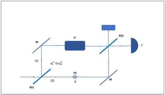
Figure 2.
Mach–Zehnder-type setup to deal with two qubits. The path-qubit, associated to the two-way alternative, plays the role of the “system” or “quanton”. A quanton’s internal qubit (spin, polarization, etc.) serves as a which-way “marker”. The unitary U acts on the marker-qubit. BS1 and BS2 are beam splitters. An unbalanced BS1 can produce path states of the form . The initial, system-marker state is available after BS1 and submitted to a non-local unitary (see text). By setting U to the identity one can address the single-qubit case.
To begin with, let us refer to inequality , as derived in [17]. The interferometric setup considered in [17] is essentially the same as that of Figure 2. The system of interest, called “quanton”, is submitted to the action of the two-way interferometer. The second system is the which-way marker, or “detector”. This marker-system is an internal DOF that is carried by the “quanton”; for example, spin in the case of neutron interferometry, or polarization in the case of photons. In order to make the marker effective, a unitary transformation U is applied to it, conditioned on the path followed by the quanton. In the case of polarization, U could be performed by three birefringent plates, set on one of the two paths (see Figure 2).
3.1. Quanton without Marker
Let us first address the quanton alone, which is submitted to the interferometer of Figure 2, with U being removed. Such a configuration is then essentially the same as the Young setup that we discussed before. The quanton goes from an initial state to a state . Here, , where represents beam splitting and phase shifting. The Pauli matrices are defined, so that , where correspond to the two paths of the interferometer. By considering the intensity pattern at one output, , we can define (fringe) visibility, as in (2): . The input state in the Young configuration corresponds to the state after the first beam-splitter in the MZ configuration: . The corresponding intensities on each arm of the interferometer are . In terms of these intensities, we define distinguishability as in (2): . This was called “predictability” in [17].
We may define Stokes parameters by writing in terms of the identity and the Pauli matrices:
Setting for brevity, the explicit expressions for the are:
where . By applying the definitions of and , i.e., those of (2) with , we get
As for the degree of polarization, , it is also easily calculated in terms of and . We can write in the form , with . Thus, the eigenvalues of are . The definition of , cf. (3), leads then to
3.2. Marker without Quanton
We now activate the marker by placing U on one arm of the interferometer. The action of the setup that is shown in Figure 2 on a system-marker initial state can be described by a unitary transformation . Here again, we can define fringe visibility in terms of the output intensity. When considering a symmetric interferometer, one obtains , with [17,33]. As for distinguishability , it may be defined in terms of the trace-distance between the two marker states, and . As shown in Ref. [17], and are mutually constrained by
According to [17], (25) and “convey utterly different messages despite their great similarity”. The reason would be that and stand for two different kinds of which-way knowledge. Englert [17] attributes the constraint on to the “positivity of the initial state of the quanton”. Instead, the constraint on would derive from “the quantum properties of the detector” [17], i.e., the marker. While the positivity of the quanton state amounts to the Hermiticity of the matrix that we mentioned before, which certainly leads to the constraint on , Englert’s statement concerning requires some qualifications. To begin with, (25) can be derived by addressing the interferometric setup of Figure 2, regardless of the quantal or classical nature that we ascribe to the carriers of the two involved DOFs, one called “quanton” and the other “marker” (or “detector”) in [17]. As shown in [33], it holds
where we have reverted to writing instead of , for the reasons we explain below. In (26), is the rotation angle that belongs to , where is a unit vector along the rotation axis. Equation (26) implies the PCT for , and, hence, also (25) with .
It might be disputed that (25) and the PCT follow from (26), because the PCT addresses one qubit, while (25) and (26) involve two qubits, the quanton and its marker. However, the actual definitions of and in [17,33] are equivalent to and , where for matrix M. The definitions of and refer then to a single qubit: the marker. This is also the case with in (26), which is given by the eigenvalues of [33]. Therefore, (26) exclusively refers to the marker qubit. The quanton (path-qubit) does not take part in this constraint.
Hence, while the marker was incorporated to store which-way information about the quanton, we end up establishing a constraint that involves the marker alone. This is a consequence of having taken the beam-splitter BS1 in Figure 2 as a symmetric one. The two paths have then equal weights. Setting an unbalanced beam-splitter BS1 and removing U lead us back to the situation already discussed, of a quanton without marker. Therefore, we need an unbalanced beam-splitter and U in place, in order to activate both quanton and marker. We do this next.
4. Two-Qubit Extension of the PCT
Our previous considerations naturally lead us to ask what happens when both the marker-qubit and the path-qubit are equally active. Let us start with the pure-mixed case, in which the path-qubit (the “system” or quanton) is in a pure state and the marker-qubit is in a mixed state. The initial, system-marker state is given by
State is available after BS1 (see Figure 2) and then submitted to the unitary transformation
Before BS2, the state of the two-qubit system is given by . The corresponding single-qubit states can be obtained by partial tracing. These states are , whose explicit form we presently do not need, and
We see that is the sum of two states, each one related to one path of the interferometer. This prompts us to define distinguishability as the trace-distance between these two states:
If the probabilities or intensities that are associated with the two paths are equal, i.e., , then reduces to the previously defined distinguishability [17]: . The definition of in (30) takes into account the two elements that contribute to distinguish one path from the other: the biased path-choice and the triggering or not of the unitary transformation.
To quantify visibility, we consider the intensity at one output of the second beam-splitter (BS2):
We then define visibility as fringe contrast, thereby obtaining
From the above expression, we obtain
Here, we use the Euler–Rodrigues parameters and , which characterize , the 3D-rotation matrix that corresponds to our . Moreover, , with , and , which is also given by the difference of the eigenvalues of matrix .
Using , we get
where and .
Equation (36) extends the PCT to the two-qubit case. It contains all of the previous results, as can be checked by setting . In this case, we must pick the first option in (36), setting and , so that . On substituting and , we obtain Equation (26), the one-qubit extension of the PCT. As we see, our generalization of the PCT comprises visibilities and distinguishabilities that refer to two qubits. While and refer to the path-qubit alone, and involve both the path-qubit and marker-qubit.
Next, we lift the restriction that the path-qubit is initially in a pure state and assume that it may be prepared, like the marker-qubit, in a mixed state. By writing the initial state of the path-qubit as a statistical mixture of pure states, we can use the above results and obtain (for details, see Appendix A):
5. Discussion
Bohr’s complementarity asserts that quantum systems may have properties that are mutually exclusive. Wave-particle duality is a prominent case of complementarity, a case that has been quantified by means of various constraints. These constraints were derived from so-called “genuinely quantum properties”. It is common scientific practice to experimentally test whatever constraints have been derived as necessary consequences of the assumed physical properties. However, problems may arise when one takes a necessary condition as being also a sufficient one, without having proved the implication in the two directions. In particular, quantumness may imply some mathematical constraint, but—unless proved otherwise—the validity of this constraint does not necessarily imply quantumness.
We have shown that several constraints that were derived in order to exhibit quantum wave-particle duality, in fact draw from interconnections between degrees of freedom that are by themselves neither quantal nor classical. Experimental tests dealing with said constraints are often conducted using quantum tools. This is perfectly valid; but, it is also valid to conduct similar tests using classical tools. What is submitted to test in such a case is, so to say, blind to the kind of employed tools.
The aforementioned, logical shortcoming has a practical consequence. By taking quantumness as a necessary condition—when it is not—for the implementation of some requirements, we can unnecessarily limit the search of possible tools needed to achieve such an implementation. Said requirements may be formulated as constraints, like those discussed in the present work, or as basic properties underlying algorithms and protocols. The latter might be the case in quantum information science.
The cases we have discussed should illustrate how often some features not really captured by a mathematical formulation can nonetheless be verbally addressed as if they were part of it. One can, for instance, refer to single photons, even though only a DOF has been mathematically encoded, a DOF that can be carried by both photons and optical light beams. One can refer to two qubits, even though all quantities entering a mathematical formulation have been defined in terms of a single qubit.
It is a pending task to lay bare the actual physical properties that enter many a mathematical formulation that has been claimed to expose genuinely quantum features. Such a task may be intimately related with the goal of achieving the so-called quantum advantage.
Funding
This material is based upon research partially supported by the Office of Naval Research under Award Number N62909-19-1-2148.
Conflicts of Interest
The author declares no conflict of interest.
Abbreviations
The following abbreviations are used in this manuscript:
| PCT | Polarization coherence theorem |
| DOF | Degree of freedom |
| LCR | Inductor, capacitor and resistor |
| MZ | Mach-Zehnder |
Appendix A
We can write the initial state of the path-qubit as a statistical mixture of pure states: , with , and . We can thus readily see that (31) generalizes to
With , we get
Here, are components of the Stokes vector that belongs to . The visibility is now given by
As for distinguishability, we define it as the statistical mixture:
Working out the above definition, we obtain
with
Equation (A6) gives . We then get
We have thus two possible cases:
For the path-qubit in the mixed state, it holds , and . Hence,
We notice that , and are joined with , and in the first equation of (A10). In the second equation instead, does not take part. However, we can rewrite this second equation as
so that now appears, while is not explicitly included.
References
- OIDA. OIDA Quantum Photonics Roadmap: Every Photon Counts. OIDA Report. 2020, Volume 3, pp. 1–70. Available online: http://www.osapublishing.org/abstract.cfm?URI=OIDA-2020-3 (accessed on 25 October 2020).
- Eberly, J.H.; Qian, X.-F.; Al Qasimi, A.; Ali, H.; Alonso, M.A.; Gutiérrez-Cuevas, R.; Little, B.J.; Howell, J.C.; Malhotra, T.; Vamivakas, A.N. Quantum and classical optics—emerging links. Phys. Scr. 2016, 91, 063003. [Google Scholar] [CrossRef]
- Wolf, E. Introduction to the Theory of Coherence and Polarization of Light; Cambridge University Press: Cambridge, UK, 2007. [Google Scholar]
- Spreeuw, R.J.C. A classical analogy of entanglement. Found. Phys. 1998, 28, 361–374. [Google Scholar] [CrossRef]
- Borges, C.V.S.; Hor-Meyll, M.; Huguenin, J.A.O.; Khoury, A.Z. Bell-like inequality for the spin-orbit separability of a laser beam. Phys. Rev. A 2010, 82, 033833. [Google Scholar] [CrossRef]
- Qian, X.-F.; Eberly, J.H. Entanglement and classical polarization states. Opt. Lett. 2011, 36, 4110–4112. [Google Scholar] [CrossRef] [PubMed]
- Kagalwala, K.H.; Di Giuseppe, G.; Abouraddy, A.F.; Saleh, E.A. Bell’s measure in classical optical coherence. Nat. Photonics 2013, 7, 72–78. [Google Scholar] [CrossRef]
- Qian, X.-F.; Little, B.; Howell, J.C.; Eberly, J.H. Shifting the quantum-classical boundary: Theory and experiment for statistically classical optical fields. Optica 2015, 2, 611–615. [Google Scholar] [CrossRef]
- Aiello, A.; Töppel, F.; Marquardt, C.; Giacobino, E.; Leuchs, G. Quantum-like nonseparable structures in optical beams. New J. Phys. 2015, 17, 043024. [Google Scholar] [CrossRef]
- McLaren, M.; Konrad, T.; Forbes, A. Measuring the nonseparability of vector vortex beams. Phys. Rev. A 2015, 92, 023833. [Google Scholar] [CrossRef]
- Gadway, B.R.; Galvez, E.J.; De Zela, F. Bell-inequality violations with single photons entangled in momentum and polarization. J. Phys. B At. Mol. Opt. Phys. 2009, 42, 015503. [Google Scholar] [CrossRef]
- Norrman, A.; Friberg, A.T.; Leuchs, G. Vector-light quantum complementarity and the degree of polarization. Optica 2020, 7, 93–97. [Google Scholar] [CrossRef]
- Qian, X.-F.; Konthasinghe, K.; Manikandan, S.K.; Spiecker, D.; Vamivakas, A.N.; Eberly, J.H. Turning off quantum duality. Phys. Rev. Res. 2020, 2, R012016. [Google Scholar] [CrossRef]
- Eberly, J.H.; Qian, X.-F.; Vamivakas, A.N. Polarization coherence theorem. Optica 2017, 4, 1113–1114. [Google Scholar] [CrossRef]
- Abouraddy, A.F.; Dogariu, A.; Saleh, B.E.A. Polarization coherence theorem: Comment. Optica 2019, 6, 829–830. [Google Scholar] [CrossRef]
- Eberly, J.H.; Qian, X.-F.; Vamivakas, A.N. Polarization coherence theorem: Reply. Optica 2019, 6, 831. [Google Scholar] [CrossRef]
- Englert, B.-G. Fringe visibility and which-way information: An inequality. Phys. Rev. Lett. 1996, 77, 2154–2157. [Google Scholar] [CrossRef]
- Greenberger, D.M.; Yasin, A. Simultaneous wave and particle knowledge in a neutron interferometer. Phys. Lett. A 1988, 128, 391. [Google Scholar] [CrossRef]
- Jaeger, G.; Shimony, A.; Vaidman, L. Two interferometric complementarities. Phys. Rev. A 1995, 51, 54. [Google Scholar] [CrossRef]
- Mandel, L. Coherence and indistinguishability. Opt. Lett. 1991, 16, 1882–1883. [Google Scholar] [CrossRef]
- Ellis, J.; Dogariu, A. Complex degree of mutual polarization. Opt. Lett. 2004, 29, 536–538. [Google Scholar] [CrossRef]
- Setälä, T.; Tervo, J.; Friberg, A.T. Stokes parameters and polarization contrasts in Young’s interference experiment. Opt. Lett. 2006, f31, 2208. [Google Scholar] [CrossRef]
- Setälä, T.; Tervo, J.; Friberg, A.T. Contrasts of Stokes parameters in Young’s interference experiment and electromagnetic degree of coherence. Opt. Lett. 2006, 31, 2669. [Google Scholar] [CrossRef] [PubMed]
- Leppänen, L.-P.; Saastamoinen, K.; Friberg, A.T.; Setälä, T. Interferometric interpretation for the degree of polarization of classical optical beams. New J. Phys. 2014, 16, 113059. [Google Scholar] [CrossRef]
- Norrman, A.; Blomstedt, K.; Setälä, T.; Friberg, A.T. Complementarity and Polarization Modulation in Photon Interference. Phys. Rev. Lett. 2017, 119, 040401. [Google Scholar] [CrossRef] [PubMed]
- Jakob, M.; Bergou, J.A. Quantitative complementarity relations in bipartite systems: Entanglement as a physical reality. Opt. Commun. 2010, 283, 827–830. [Google Scholar] [CrossRef]
- Wootters, W.K. Entanglement of Formation of an Arbitrary State of Two Qubits. Phys. Rev. Lett. 1998, 80, 2245–2248. [Google Scholar] [CrossRef]
- Qian, X.-F.; Malhotra, T.; Vamivakas, A.N.; Eberly, J.H. Coherence constraints and the last hidden optical coherence. Phys. Rev. Lett. 2016, 117, 153901. [Google Scholar] [CrossRef]
- Eberly, J.H. Correlation, coherence and context. Laser Phys. 2016, 26, 084004. [Google Scholar] [CrossRef]
- Qian, X.-F.; Vamivakas, A.N.; Eberly, J.H. Entanglement limits duality and vice versa. Optica 2018, 5, 942–947. [Google Scholar] [CrossRef]
- De Zela, F. Optical approach to concurrence and polarization. Opt. Lett. 2018, 43, 2603–2606. [Google Scholar] [CrossRef]
- James, D.F.V.; Kwiat, P.G.; Munro, W.J.; White, A.G. Measurement of qubits. Phys. Rev. A 2001, 64, 052312. [Google Scholar] [CrossRef]
- De Zela, F. Hidden coherences and two-state systems. Optica 2018, 5, 243–250. [Google Scholar] [CrossRef]
Publisher’s Note: MDPI stays neutral with regard to jurisdictional claims in published maps and institutional affiliations. |
© 2020 by the author. Licensee MDPI, Basel, Switzerland. This article is an open access article distributed under the terms and conditions of the Creative Commons Attribution (CC BY) license (http://creativecommons.org/licenses/by/4.0/).