Review

Casimir Effect with Dielectric Matter in Salted Water and Implications at the Cell Scale


1
Centre of Excellence ENSEMBLE3, Sp. z o. o., Wolczynska Str. 133, 01-919 Warsaw, Poland
2
Instituto de Física, Universidade Federal do Rio de Janeiro, Rio de Janeiro 21941-972, Brazil
3
Forschungszentrum Jülich, 52425 Jülich, Germany
4
RWTH (Rhine-Westphalian Academy of Sciences), Aachen University, 52062 Aachen, Germany
5
Laboratoire Kastler Brossel, Sorbonne Université, CNRS (Centre National de la Recherche Scientifique), ENS-PSL (École Normale Supérieure, Université Paris Sciences et Lettres), Collège de France, 75252 Paris, France
*
Authors to whom correspondence should be addressed.
Physics 2026, 8(2), 40; https://doi.org/10.3390/physics8020040
Submission received: 13 January 2026 / Revised: 13 February 2026 / Accepted: 28 February 2026 / Published: 10 April 2026

Abstract

The Casimir interaction in salted water contains a universal contribution of electromagnetic fluctuations that makes it of a longer range than previously thought. The universal contribution dominates non-universal ones at the distances relevant for actin fibers inside the cell. We discuss universal and non-universal contributions with a model mimicking biological matter. We also show that the universal Casimir effect should have crucial implications at the cell scale.

1. Introduction

Quantum physics was born when Max Planck wrote the first quantum law, where he explained the properties of black-body radiation [1] (English translation in Ref. [2]). This law gave the mean energy per mode of the electromagnetic field as the product of the energy of a photon ω , with the reduced Planck constant, and a mean number n ¯ ω of thermal photons per mode at frequency ω . Approximately ten years later, Planck [3] added an extra term 1 2 ω to the mean energy per mode. This marked the appearance in physics of zero-point fluctuations, which have superseded the now abandoned reasoning of the paper in which they were introduced [4,5].
While the original Planck’s law fell off the expectation k B T , with k B the Boltzmann constant, by a constant offset ω / 2 at high temperatures ( T ), the second law including zero-point fluctuations had the correct classical limit [6] (English translation in Ref. [7]). The modern writing of the mean energy per mode makes this property straightforward since all the terms in the high-temperature expansion go to 0 at T but the dominant one,
1 2 + n ¯ ω ω = ω 2 coth ω 2 k B T T k B T + 𝒪 1 T .
Discussions on zero-point fluctuations were active before their precise nature was better understood as the full development of quantum theory took place [8]. Vacuum fluctuations, the zero-point fluctuations of electromagnetic fields in empty space, were introduced in previous quantum theory [9,10].
Nowadays, zero-point fluctuations are considered as a consequence of the non-commutative character of quantum observables [11,12,13,14] (these papers are reproduced or English-translated, and commented in Ref. [15]). The dispersions of these fluctuations are specified by inequalities deduced from the commutators of observables [16] (English translation in Ref. [17]; history is discussed, for example, in Refs. [18,19,20]). Vacuum fluctuations are now defined by the quantum theory of the electromagnetic field [21], with each field mode represented by canonical variables analogous to those of an harmonic oscillator. This theory leads to a full quantum derivation of Einstein’s description of absorption, stimulated and spontaneous emission processes [22] (English translation in Ref. [23]). Vacuum fluctuations have many essential effects in atomic and subatomic physics, such as the Lamb shift and radiative corrections [24,25,26,27,28].
In this paper, we focus the discussions on mechanical effects due to the radiation pressure of these fluctuations that are Casimir forces [29] and related Casimir–Polder and van der Waals forces [30,31,32]. In his initial study, Hendrik Casimir studied an idealized problem with two perfectly reflecting plane mirrors in an electromagnetic vacuum at zero temperature. Since then, a considerable number of papers have generalized the description to make it more realistic in terms of material properties and geometry (a review with many references can be found in Ref. [33]). Meanwhile, more and more sophisticated experiments have, in particular, precisely measured the forces between metallic reflecting surfaces in empty space (reviews and references in Refs. [34,35,36,37,38,39]).
We stress at this point that most experiments are performed at room temperature, so thermal and zero-point fluctuations have to be considered together. The study of the Casimir effect in the presence of thermal fluctuations has a long history [40,41,42]. It is conveniently addressed by using the Matsubara summation technique [43]. The latter is directly related to Equation (1) as Matsubara frequencies ξ n are nothing but the poles of the hyperbolic cotangent function, namely [44]
1 2 coth ω 2 k B T = n = + k B T ω 𝚤 ξ n , ξ n = n 2 π k B T .
An advantage of the Matsubara technique is that the high-temperature limit of the interaction is given by the term at zero frequency, that is, the pole at ω = 0 in the formulas (1) and (2). This contribution has a universal character [45,46] since it does not depend on details of the variation with frequency of the electromagnetic response functions (details discussed below).
For the most common experimental configuration using metallic scatterers in empty space (see [46] and the references therein), this universal limit can only be met at distances larger than the thermal wavelength in vacuum, where the force is quite small and hard to measure with precision (see the experiments discussed in Refs. [47,48]). There exists, however, another configuration of great interest in this respect, which involves dielectric matter in electrolytes. In this case, the Casimir force can be both large and dominated by the universal term at distances that are not too large. This configuration has been studied in previous theoretical and experimental papers [49,50,51,52,53] and is reviewed in the following.
This universal Casimir effect in electrolytes is of particular relevance at the interface of physics and biology as it may have quite a large impact on the mechanics of biological systems at the cell scale, a point that has been recently emphasized [54] and is revisited below.

2. Scattering Theory of Casimir Interaction in Electrolytes

We first describe in this Section the scattering theory of the Casimir effect in electrolytes in the simplest geometry of two bulks of matter with parallel plane interfaces, separated by an electrolyte layer [50]; see Figure 1.
As we consider the Casimir interaction between objects immersed in an electrolyte, the key “novelty” is that the dissolved ions give rise to essential nonlocal effects. Such nonlocality, also referred to as spatial dispersion, manifests itself in a wave number k-dependence of the permittivity in reciprocal space and also in the emergence of a nontrivial tensorial character of the electrolyte permittivity
ϵ ( ω ) ϵ i j ( ω , k ) ,
where i j denote the tensor indexes. The main consequence of the nonlocality of the medium is the support of longitudinal modes, in addition to the standard transverse electromagnetic fluctuations. The medium allows for three independent polarizations: transverse electric (TE), transverse magnetic (TM) and longitudinal (), and the extra degree of freedom for the fluctuations has considerable consequences for dispersion interactions [50].
The most economical way of writing the Casimir energy is by reinterpreting it as a reverberation problem for the electromagnetic fluctuations and then making a Wick rotation to imaginary frequencies [44]. For simplicity, let us assume that the bulk materials are strictly (spatially) local. The Wick rotation produces a Matsubara sum over the frequencies defined in Equation (2)
F Cas = F 0 + n = 1 F n .
In the total Casimir free energy (4), we separate the term F 0 , corresponding to the zero Matsubara frequency, as it plays the main role in the discussions of this paper. The other terms F n , each corresponding to a nonzero frequency ξ n , are discussed for the two-bulk geometry in Ref. [50], and they are discussed for the two-slab geometry in Section 5 below.
It can be shown [50] that the TM and fluctuations are coupled at the interfaces between the bulks and medium, but, in effect, it turns out that the TE term vanishes in the limit ξ 0 and the TM- contributions actually uncouple one from another [55], thus yielding for an area A:
F 0 = A k B T 2 d 2 k ( 2 π ) 2 ln 1 e 2 k d A k B T 16 π ζ ( 3 ) d 2 + A k B T 2 d 2 k ( 2 π ) 2 ln 1 r 2 e 2 k 2 + λ D 2 d F 0 ( ) ,
with r the reflection amplitde and λ D the Debye length. Let us rewrite expression (5) by highlighting the first (TM) term that is henceforth referred to as the universal Casimir contribution F univ bulk as it depends only on the temperature and geometry:
F 0 = F univ bulk + F 0 ( ) , F univ bulk = A H 12 π d 2 , H = 3 ζ ( 3 ) 4 k B T .
The Hamaker constant H depends only on temperature ( H 0.9 k B T , with ζ denoting the Riemann function and ζ ( 3 ) 1.202 the Apery’s constant), and it yields F through a multiplication by a dimensionless geometrical quantity. As F univ bulk is proportional to temperature, the associated entropy is deduced just to be such that the mechanical energy F univ bulk + T S univ bulk , where S univ bulk denotes the entropy, vanishes, which means that the universal Casimir interaction is a purely entropic effect. These properties are still true for the other geometries considered below, with different expressions, naturally.
The second term in Equation (5) is the longitudinal contribution at zero Matsubara frequency, and is determined by the reflection amplitude r and the Debye length, λ D :
r = ϵ b ( 0 ) k 2 + λ D 2 ϵ 2 ( 0 ) k ϵ b ( 0 ) k 2 + λ D 2 + ϵ 2 ( 0 ) k , λ D = ϵ b ( 0 ) k B T n 2 m ,
respectively, where n is the ionic concentration in the electrolyte, m is the ion mass, and ϵ b is the dielectric permittivity of pure water (i.e., the permittivity of water without the ionic contribution).
In the long-distance limit, the longitudinal part F 0 ( ) is exponentially suppressed by the Debye screening with typical length λ D
F 0 ( ) e 2 d / λ D .
This is the first major takeaway of this paper: there is indeed a screening of the contribution F 0 ( ) of longitudinal modes across the electrolyte, but the universal contribution F univ bulk is unscreened as it arises from the transverse electromagnetic fluctuations. This property was first demonstrated in the framework of a macroscopic description of the dielectric response of salted water [50], and it has been confirmed since then by the molecular dynamics simulations presented in Ref. [54]. This has far-reaching consequences for physical and even biological systems, which we discuss below.
An essential aspect has to be clarified at this point. The discussions just presented on transverse and longitudinal fluctuations treat fields in the vicinity of zero frequency rather than at zero frequency. In technical terms, what was calculated is given by a residue associated with the pole at ω = 0 of the cotangent function in Equation (2). The physical origin of the effect is merely the divergence as k B T / ( ω ) of the number of photons in a field mode with frequency close to ω = 0 , finally resulting in a finite contribution to the free energy.

3. Experimental Evidence with Optical Tweezers

Optical tweezers [56] are considered a highly appropriate tool to measure interaction forces in aqueous media, and several applications in biology have been developed [57,58]. Since the trap stiffness is proportional to the beam laser power, the system can be tuned to match the required order of magnitude. Standard single-beam traps are most effective for particles whose refractive indexes are slightly higher than that of the surrounding medium. Conveniently, this is also the condition that minimizes the non-universal contributions F n 1 , which depend on the reflection (or more generally scattering) amplitudes at the interface between the material and the host medium.
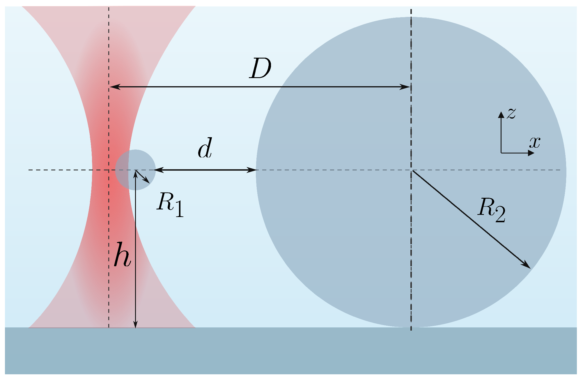
The universal Casimir interaction between two silica microspheres immersed in salted water has been measured with optical tweezers [51]. The experimental scheme is sketched in Figure 2. Brownian fluctuations of a small silica microsphere (radius R 1 = 2.4 μ m ) held by optical tweezers were measured along the x and y directions transverse to the laser beam. The interaction energy was then observed through the modification of the fluctuations along the x-axis connecting the sphere centers as the larger microsphere (radius R 2 = 12 μ m ), adhered to the glass slide at the bottom of the sample, was approached by employing a piezoelectric nano-positioning system. The sample was also displaced vertically to align the sphere centers so as to have h = R 2 , where h is the height of the small microsphere with respect to the glass slide. While fluctuations along x captured the interaction signal, fluctuations along y were not modified, showing the absence of optical binding or of any other perturbation of the optical force in this configuration with near-index matching. Since the trapping beam was circularly polarized, the Brownian fluctuations along y accumulated over several experimental runs were employed to infer the optical potential relevant for the interaction direction x . As an additional check, the resulting optical potential was shown to agree with the Mie–Debye theory of optical tweezers [59,60] as well as with standard Stokes calibration [61], with the latter implemented in the absence of the larger microsphere.
The interaction energy for distances above 100 nm was then obtained by subtracting the optical potential from the total energy as determined by the Brownian dynamics along the x-direction. For moderate salt concentrations, the interaction was dominated by the electrostatic double-layer interaction. In order to suppress such interaction, a second experiment reported in Ref. [51] employed a high salt concentration (strong screening with λ D = 0.65 nm ). In this second case, the interaction was completely dominated by the universal Casimir contribution discussed in the previous section.
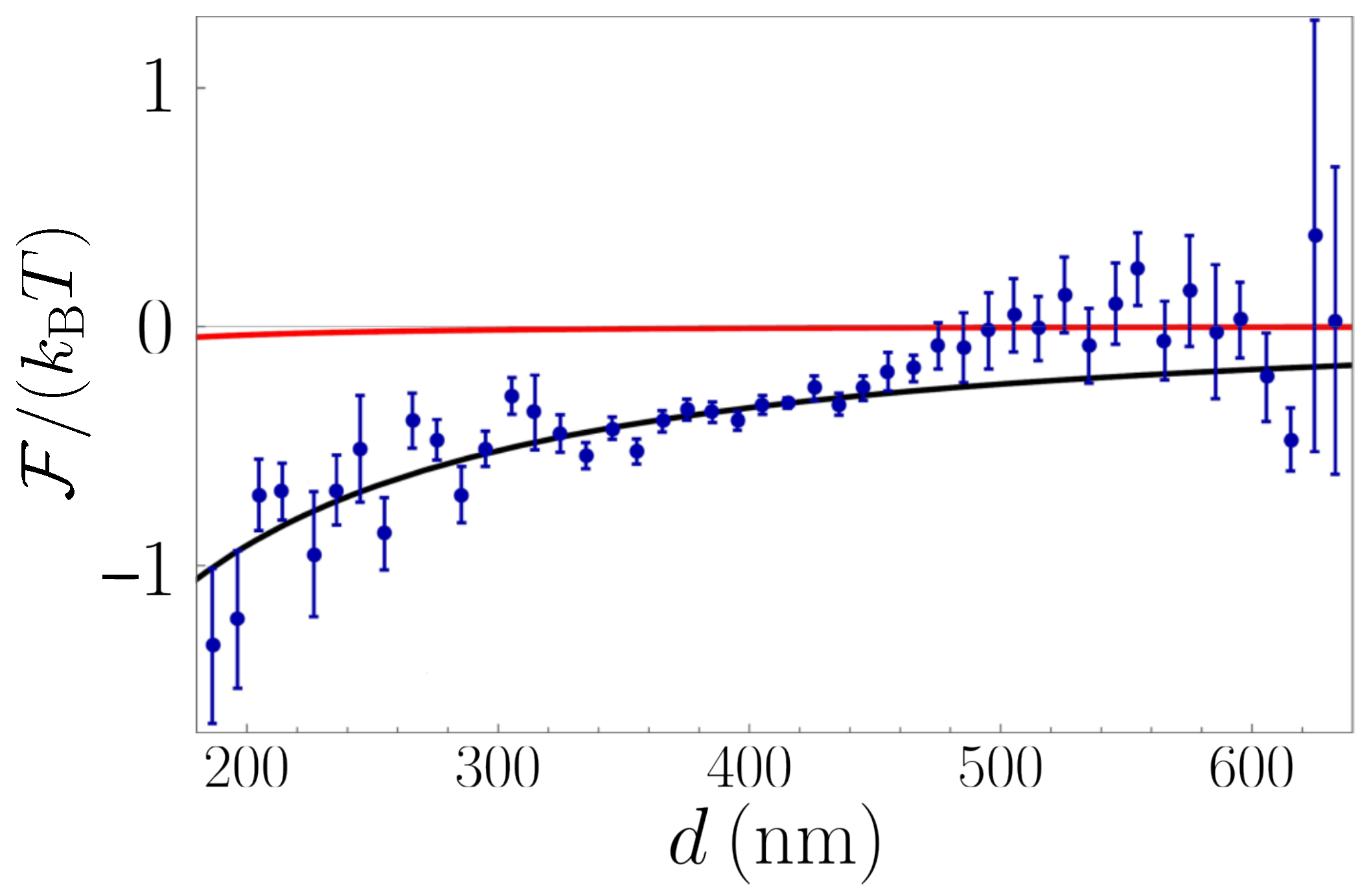
Figure 3 shows the resulting Casimir energy in units of k B T versus distance d of closest approach (see Figure 2). The red curve represents the non-universal contribution accounting for the positive Matsubara frequencies ξ n 1 . The calculation is based on Mie scattering by dielectric spheres in water [62]. The red curve thus represents the generalization for the geometry of two spheres of the standard theoretical prediction for the Casimir interaction in salted water [32], which is often considered within the parallel planar interface setup or within the corresponding proximity-force approximation. The longitudinal contribution F 0 ( ) is not included as it is negligible at both moderate and high salt concentrations employed in Ref. [51] due to the fact that the distances are much larger than the corresponding Debye screening lengths. Indeed, F 0 ( ) is given by the second term on the right-hand side of Equation (5) for parallel planar interfaces and calculated for two spheres in Ref. [63]. In both cases, F 0 ( ) becomes exponentially small at distances larger than λ D .
The black curve in Figure 3 shows the total Casimir interaction, including the universal contribution arising from TM modes in the zero-frequency limit. Like the non-universal contribution, the total Casimir interaction is calculated exactly for the geometry of two dielectric spheres in salted water as described in Refs. [52,53] (see also Section 4 below). The comparison between the black and red curves indicates that the universal contribution dominates the Casimir interaction for distances above 200 nm . More importantly, the unscreened universal Casimir contribution provides an excellent description of the data, with no fitting parameter, in contrast with the standard approach that overlooks the contribution of TM modes and is excluded by the experimental data shown in Figure 3.

4. Universal Casimir Interaction in the Two-Sphere or Two-Cylinder Geometries

The universal Casimir interaction that is the high-temperature limit of the expression in the case of highly efficient Debye screening has been calculated in the two-sphere [52,53] and two-cylinder [54] geometries. As in the two-bulk geometry considered above, it arises from the term n = 0 in the Matsubara sum appearing due to transverse electromagnetic fluctuations, and it does not depend on details of the frequency dependence of dielectric functions.
The associated free energy is the product of the thermal energy scale k B T by a dimensionless function f, which now depends in a nontrivial manner on the geometrical parameters. In the two-sphere geometry, we have
F univ sph = k B T f d , R 1 , R 2 .
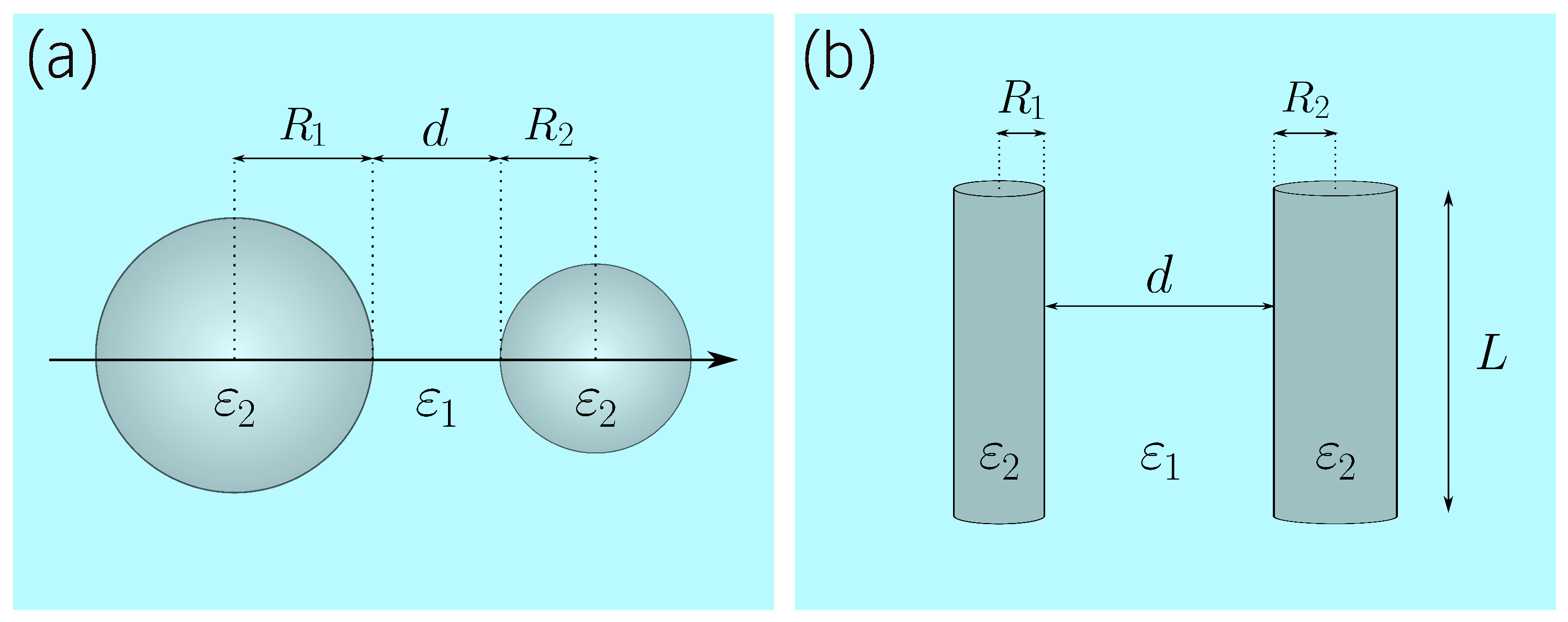
The Casimir interaction is captured in the function f, which has been calculated for two dielectric spheres in salted water [52,53]. The function f does not depend on temperature (the effect is purely entropic), and it is a dimensionless function of the two ratios that can be formed with the three length parameters d (note that it was denoted L in Refs. [52,53]), R 1 and R 2 (radii of the two spheres; see Figure 4a).
The function f is calculated within the scattering theory of the Casimir effect [44]. It is a sum over all field modes of scattering operators involving an arbitrary number of round-trips in the cavity formed by the two objects. In the so-called dipolar limit where the spheres have small sizes in comparison with the distance, the contributions of large numbers of round-trips are negligible. In this small-size approximation (SSA) or equivalently long-distance approximation, f is proportional to the two volumes R 1 3 and R 2 3 , and inversely proportional to the sixth power of distance [52,53]:
f SSA = 3 R 1 3 R 2 3 4 d 6 .
In the opposite limit of a short distance between the spheres, the exact result involves large numbers of round-trips, and it tends to an expression related to the two-bulk geometry through the proximity-force approximation (PFA) [64]. In this PFA limit, f is proportional to the effective radius R eff defined from the two radii R 1 and R 2 , and inversely proportional to the distance
f PFA = ζ ( 3 ) R eff 8 d and R eff = R 1 R 2 R 1 + R 2 .
The function f has a universal expression that does not depend on the details of the variation with frequency of the permittivity functions of either the dielectric matter in the spheres or salted water constituting the immersion medium. The result is conveniently conveyed—just like in Figure 1(b) of Ref. [52]—as a function f u x of two dimensionless parameters
x = d R eff and u = R 1 R 2 R 1 + R 2 2 ,
where x is an aspect ratio for the distance d and u an aspect ratio for the radii. Further, f depends only on x, and u is a remarkable scale-invariance property, meaning that f is unchanged when the three geometrical dimensions d , R 1 , and R 2 are multiplied by a common factor.
A more subtle property appears when f is written (see Figure 2 of Ref. [52]) in terms of another parameter,
y = d + R 1 + R 2 2 + R 1 2 + R 2 2 2 R 1 R 2 = 1 + x 1 + u x 2 .
The value of f thus appears to depend mainly on y, which reveals an approximate conformal invariance of geometrical dependence of the free energy [52,53]. This property has been used in Ref. [53] to provide a relatively simple formula that can be applied to a wide range of geometrical parameters. This formula is sufficient for the salinity of biological media and at ambient temperature. The obtained free energy F univ sph is larger than k B T ( f 1 ) only for spheres quite close one to another, that is, the geometry in which the universal Casimir interaction has been experimentally measured (see Section 3).
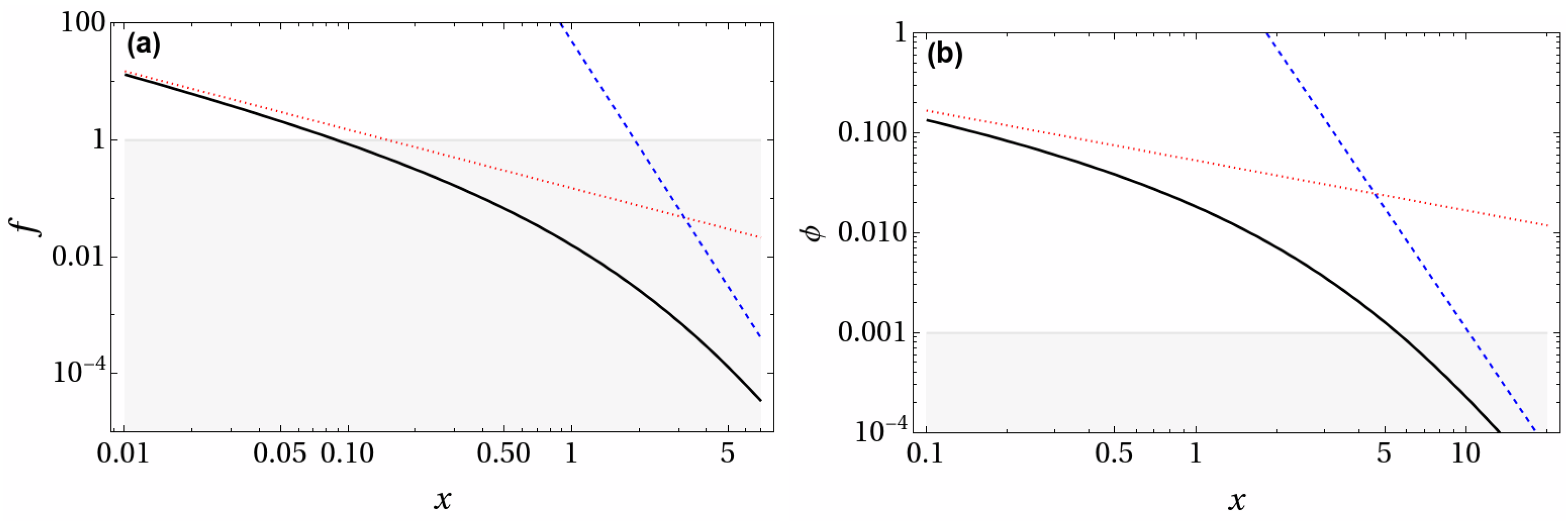
In order to compare the two-sphere case and the two-cylinder one discussed below, we consider the geometry of two spheres with equal radii R 1 = R 2 = R and show in Figure 5a the corresponding function f versus the geometric parameter x defined in (12). The grayed out band in the figure shows where f < 1 , which is also where the binding energy | F | is smaller than the Brownian motion energy scale. Figure 5a shows that the universal Casimir effect dominates the Brownian energy k B T for distances d < 0.09 R eff . Note that, for the geometry with different radii employed in the optical tweezers experiment of Section 3, the order of magnitude for this border | F univ sph | k B T is at d 0.2 μ m , which is indeed the scale of distances probed in Ref. [51].
We now come to the discussion of the configuration with two dielectric cylinders in salted water. This configuration makes the interaction larger than in the two-sphere case as it scales as the length L of the cylinders. The geometry is shown in Figure 4b with two cylinders with radii R 1 and R 2 at a distance d of closest approach. In this geometry, the universal Casimir free energy is the product of the thermal energy k B T by two dimensionless factors L / d and ϕ
F univ cyl = k B T L d ϕ d , R 1 , R 2 .
The physics of the universal interaction is captured in the function ϕ , which has been calculated in Ref. [54]. The remarks just after Equation (9) remain valid here as soon as ϕ does not depend on temperature and is a dimensionless function of two ratios of the three geometrical quantities d , R 1 and R 2 .
In order to discuss the implications of these results for biological systems in Section 6, we depict in Figure 5b the function ϕ for two cylinders with equal radii R 1 = R 2 = R . The function ϕ is plotted versus the geometric parameter x defined as in Equation (12) but for cylinders. The grayed out band in the figure shows where ϕ < 0.001 , that is, where the binding energy | F | is smaller than the Brownian motion energy scale for L = 1000 d (see the discussions in Section 6 below). The key message from Figure 5b is that the universal Casimir free energy dominates the Brownian motion energy k B T imposed by the surrounding water over a broad range of parameters, including in particular distances d of the order of R eff . The striking difference between the two-sphere case (Figure 5a) and the two-cylinder one (Figure 5b) is just due to the presence of the considerably large factor L / d in Equation (14), which makes | F univ cyl | larger than k B T in a wider range of parameters.
Both functions—f and ϕ —in Figure 5 agree with the proximity-force approximation (red dotted curve) at short separations and with the small-size approximation (blue dashed line) at long distances. For completeness, we give the PFA and SSA expressions for the case of two cylinders:
ϕ PFA = ζ ( 3 ) 32 2 R eff d and ϕ SSA = 891 π 4096 R 1 2 R 2 2 d 4 ,
respectively. The expressions (15) to be compared with Equations (11) and (10), respectively. In particular, the power-law changes have clear meanings. For the PFA, ϕ is proportional to R eff / d because there is only one curvature radius in a direction orthogonal to the distance for cylinders (there are two of them for spheres, and f is proportional to R eff / d ). For the SSA, the extensive quantity in the perturbative limit is the area for cylinders rather than the volume for spheres. It follows that ϕ is proportional to the two areas R 1 2 and R 2 2 and inversely proportional to the fourth power of distance.

5. Non-Universal Contributions with Dielectric Matter in Salted Water

The universal Casimir interaction was calculated in Ref. [54] for two dielectric cylinders in salted water, but the non-universal contributions have never been analyzed in this geometry. In order to fill this gap, one needs a robust model for the dielectric response of matter as non-universal contributions depend on this response. In the absence of an exact solution, we have also to produce a reasonably accurate estimate for the interaction between two cylinders. These requirements are tackled in this Section.
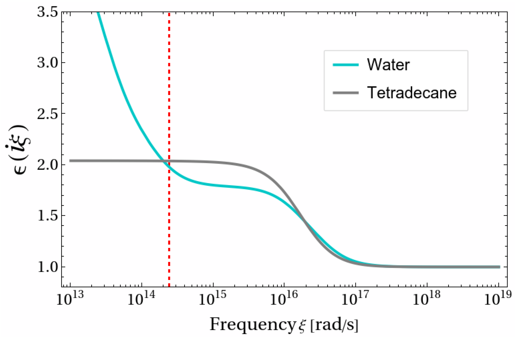
For describing dielectric properties of organic matter, we follow Refs. [65,66] by considering tetradecane as a proxy for these properties. Its dielectric function is given by a Lorentz model, with parameters to be found in [67]. In addition, we modelled salted water as in Refs. [50,55], with the contribution from the ions depending on their concentration. As we mentioned in Section 4 above, this contribution is critical for the universal contribution at zero frequency, but it plays a negligible role at nonzero Matsubara frequencies, which are way large (at room temperature) to “feel” the effect of ionic conduction (when compared to electrons, ions have a much larger mass and their number per unit volume is much smaller). The tetradecane function is represented in Figure 6 versus imaginary frequency ω = 𝚤 ξ (i.e., after a Wick rotation, as is common for studies of the Casimir effect [33]), alongside the pure water function (i.e., disregarding the ionic contribution) taken from the model in Ref. [68]. The vertical dashed line in Figure 6 shows the position of the first nonzero Matsubara frequency ξ 1 at room temperature. The figure indicates a nearly perfect index matching of biological matter and water at this frequency, which is at the root of the smallness of the non-universal contributions to the Casimir interaction. Although the contribution of ions is negligible at this frequency, the index contrast grows sharply for lower frequencies, in particular as the effective response diverges for salted water. This Drude-like divergence caused by the dissolved ions is the reason why the universal contribution ends up not depending on the details of the properties of the material immersed in salted water.
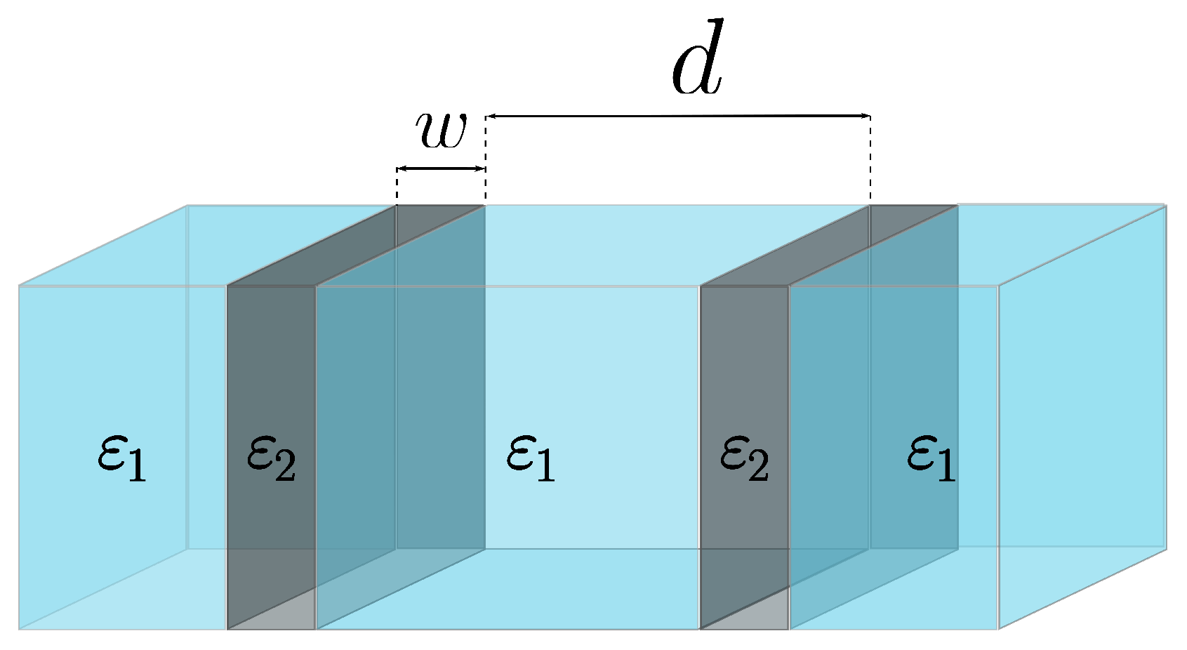
In order to get reliable estimations for the non-universal contributions to interaction between cylinders, we use the fact that these contributions are considered to be comparably small due to the index-matching at most non-null Matsubara frequencies and, therefore, that they should be approximately represented by a pairwise summation technique [69]. Let us stress that such an approximation cannot give an accurate description of the universal contribution as perturbation theory is in no way adapted to this case. Guided by the pairwise summation, we consider that the order of magnitude of the ratio between universal and non-universal contributions arising from two cylinders of radii R can be approximately estimated from the same calculation in a setup of two slabs of thickness w 2 R separated by a gap d of salted water (see Figure 7).
Rewriting expression (4) for slabs, we get
F Cas slab = F 0 slab + n = 1 F n slab .
where the nonzero Matsubara terms are given by
F n slab = A k B T σ d 2 k ( 2 π ) 2 ln 1 r ˜ ( σ ) ( 𝚤 ξ n ) 2 e 2 κ 1 d , n 0 ,
with σ representing either TE or TM polarization of a given electromagnetic mode. Here, the reflection coefficients of a slab are given by [70]
r ˜ ( σ ) ( 𝚤 ξ n ) = r ( σ ) ( 𝚤 ξ n ) 1 exp ( 2 κ 2 w ) 1 r ( σ ) ( 𝚤 ξ n ) 2 exp ( 2 κ 2 w ) and κ i = ϵ i ( 𝚤 ξ n ) ξ n 2 / c 2 + k 2 ,
where c is the speed of light and r ( σ ) ( 𝚤 ξ n ) are the Fresnel coefficients for a plane wave going from the electrolyte to the slab
r ( TE ) ( 𝚤 ξ n ) = κ 1 κ 2 κ 1 + κ 2 , r ( TM ) ( 𝚤 ξ n ) = ε 2 κ 1 ε 1 κ 2 ε 2 κ 1 + ε 1 κ 2 .
The zero-frequency Matsubara term F 0 slab for the slabs is analogous to expression (5). Given that we are interested in the distances d λ D , the longitudinal part is negligible:
F 0 slab F univ slab .
As shown in the Appendix of Ref. [55], the universal contribution for two slabs is the same as in the case of two half-spaces discussed in Section 2: F univ slab = F univ bulk .
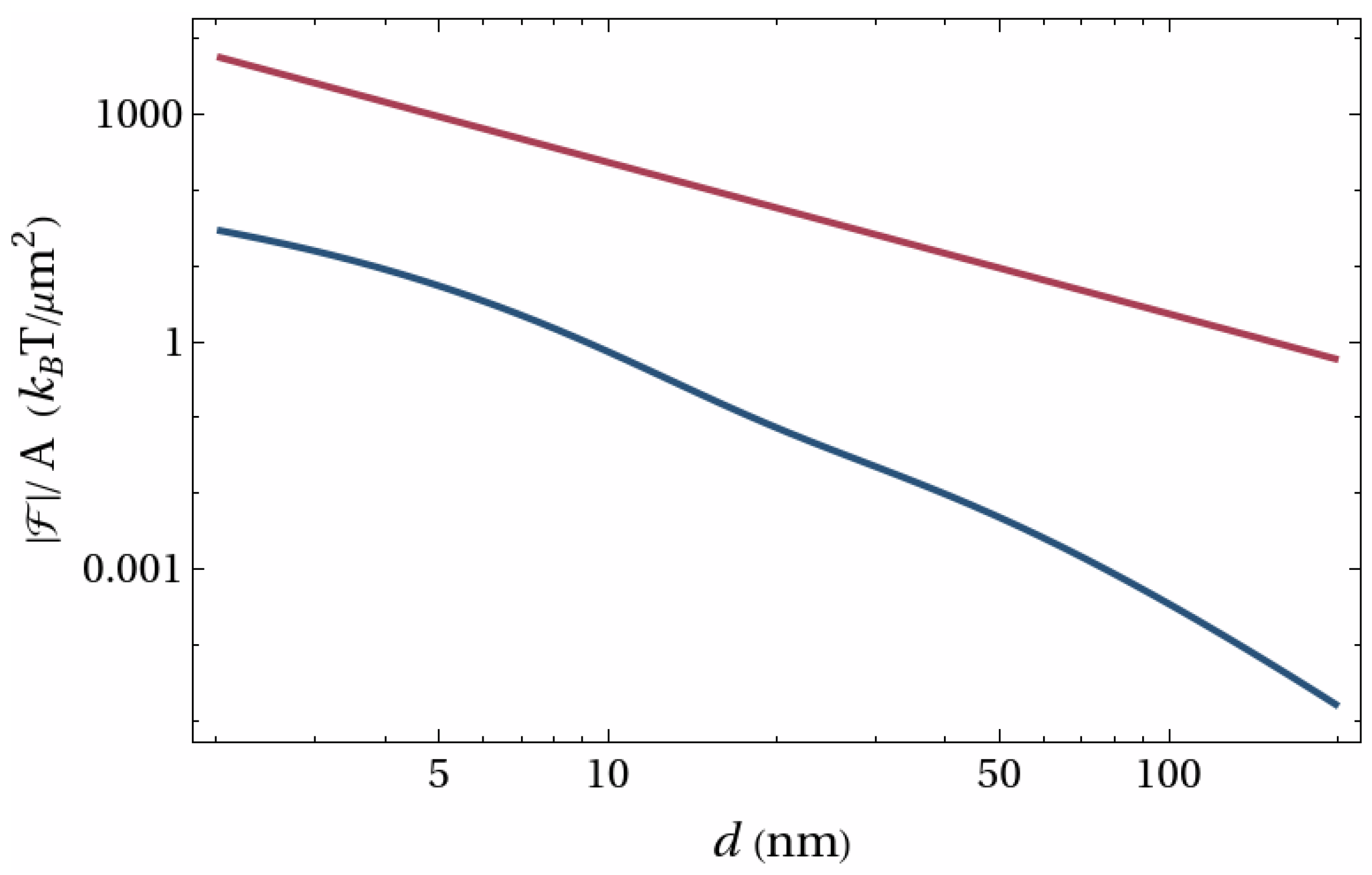
The variations in the universal contribution for the binding energy | F univ slab | and the non-universal part | n 1 F n slab | versus distance d are depicted separately in Figure 8, for identical slabs of thickness w = 6 nm (this number is motivated by discussions in Section 6). The non-universal contributions have been calculated with the dielectric model for tetradecane represented in Figure 6. Figure 8 clearly shows that the non-universal contributions are much smaller than the universal one, which is a consequence of the index-matching at nonzero Matsubara frequencies between water and tetradecane. We have checked that the ratio between the two contributions is always above a factor 100.

6. Implications at the Cell Scale

We now use the results obtained to show how the universal Casimir interaction may play an essential role in biomechanics at the cell scale. The question was thoroughly discussed in Ref. [54], where many references can be found. Here, we only recall a few critical points.
Actin filaments play critical roles in the mechanical functions of the cytoskeleton, as well as in many intracellular processes, by actively generating forces with the help of motor proteins [71,72,73]. The actin filaments form bundles, with filaments cross-linked by specific proteins into parallel arrays. It has been shown that bundles of parallel filaments may form in vitro in the absence of cross-linkers [74,75]. Other examples of self-assembled filaments are discussed in Ref. [54], which play key roles in or beyond the cytoskeleton. The universal Casimir interaction considered in this paper is relevant at the observed dimensions for bundles of actin filaments, so it should have essential implications in the self-assembly and cohesion of bundles of filaments at the cell scale.
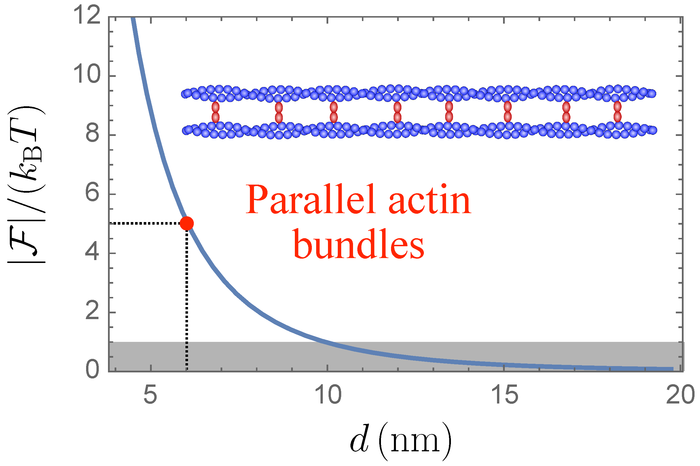
Estimation of the interaction for the relevant case of parallel actin filaments is conducted by modeling filaments as cylinders and using the physical dimensions known for parallel actin filaments [76], each having a radius R 3 nm and a length L 15 μm, which form bundles with a typical distance of closest approach d 6 nm between filaments (geometry sketched as an inset in Figure 9, with filaments shown in blue and cross-linkers in red). Such distance is about ten times larger than the characteristic Debye screening length λ D in biologically relevant solutions. The electrostatic interaction as well as the longitudinal contribution to the Casimir interaction (see Section 2) are then negligible as they are efficiently screened. The parameters given above correspond to a large value for the ratio L / d 2500 , which is a key reason that the corresponding Casimir interaction is as significant. The binding energy | F | , expressed in units of k B T , is shown versus the separation distance d in Figure 9. The relevant distance, d 6 nm, is emphasized as the red point, where the binding energy is of the order of 5 k B T . In the gray-shaded zone, | F | is dominated by the Brownian motion energy k B T .
Let us stress at this point that such a magnitude had to be expected for a physical interaction having relevance for biomechanics at the cell scale. The interaction has to be larger than k B T in order to dominate Brownian agitation, while it should not be way large to be compatible with mechanical activity provided by molecular motors. This was underlined by Moysés Nussenzveig in his remarkable paper [57] commenting on the links between physics and biology, and discussing in particular the pioneering studies by Niels Bohr [77] and Erwin Schrödinger [78].
We also emphasize that this magnitude has been obtained without any ad hoc fine-tuning of the parameters. The energy constants are given by the theory of the universal Casimir interaction reviewed in this paper, and they do not depend on any specific detail of the biological matter involved. Hence, the binding energy depends only on geometrical parameters known for bundles of actin filaments [76]. Note also that the numbers presented for actin (red solid dot in Figure 9) correspond to x = 4 in Figure 5b, where the PFA expression overestimates the correct value of ϕ by a factor of 13 . This implies that the calculation presented in Ref. [54] for cylinders was mandatory for obtaining a reliable estimation for bundles of actin filaments.
Another crucial point becomes clearer after the discussions in the present paper. We gave here an estimation of the non-universal Casimir interaction in Section 5, showing that it is more than a hundred times smaller than the universal one. For the relevant distance d = 6 nm between actin filaments, the non-universal contribution is then smaller than 0.05   k B T . It is thus established that the non-universal interaction is not only much smaller than the universal one but also way too small to have any relevance in a medium dominated by Brownian agitation. It is only the presence of the universal contribution that makes the Casimir binding energy essential for biomechanics at the cell scale.
As a concluding remark, let us stress that physics is highly complex at the cell scale, with quite a large number of different processes involved in the mechanics and functionalities of the cell. Detailed discussions of this crucial point are presented in the concluding part of Ref. [54]. Our modest aim in this review has been to show that the universal Casimir interaction due to transverse electromagnetic fluctuations has to be considered as a significant contribution to this rich physics as it produces an attractive interaction between biological filaments in the cell with a typical energy of a few Brownian thermal scales k B T .

Author Contributions

All authors have contributed to the various aspects involved in the writing of this review. All authors have read and agreed to the published version of the manuscript.

Funding

This work was supported by CAPES-COFECUB (Coordenação de Aperfeiçoamento de Pessoal de Nível Superior -, Comité français d’Evaluation de la Coopération universitaire et scientifique avec le Brésil) collaboration project n° Ph1030/24, Conselho Nacional de Desenvolvimento Científico e Tecnológico (CNPq-Brazil), Instituto Nacional de Ciência e Tecnologia de Fluidos Complexos (INCT-FCx), and the Research Foundations of the States of Rio de Janeiro (FAPERJ) and São Paulo (FAPESP), Brazil. L.I. was supported by project No. 2022/47/P/ST3/01236, co-funded by the National Science Centre and the European Union’s Horizon 2020 research and innovation program under Marie Skłodowska-Curie grant agreement No. 945339. Institutional and infrastructural support for the ENSEMBLE3 Centre of Excellence was provided through the ENSEMBLE3 project (MAB/2020/14), delivered within the Foundation for Polish Science International Research Agenda Programme and co-financed by the European Regional Development Fund and the Horizon 2020 Teaming for Excellence initiative (Grant Agreement No. 857543), as well as the Ministry of Education and Science initiative “Support for Centres of Excellence in Poland under Horizon 2020” (MEiN/2023/DIR/3797).

Data Availability Statement

No new data were created.

Acknowledgments

This paper is dedicated to the memory of our dear and esteemed colleague, H. Moysés Nussenzveig, to whom we are indebted for many inspiring discussions. The authors warmly thank the colleagues who have participated in the development of this project over the years, in particular D.S. Ether, L.B. Pires, S. Umrath, D. Martinez, Y. Ayala, B. Pontes, G.R.S. Araújo, S. Frases, G.-L. Ingold, N.B. Viana, R.O. Nunes, A.B. Moraes, A. Canaguier-Durand, R. Guérout, B. Spreng, M.J.B. Moura, R.S. Decca, R.S. Dutra, M. Borges, T. Schoger, H. Berthoumieux, and A.-F. Bitbol.

Conflicts of Interest

The authors declare no conflicts of interest.

References

  1. Planck, M. Zur Theorie des Gesetzes der Energieverteilung im Normalspektrum. Verhandl. Deutsch. Phys. Gesellsch. 1900, 2, 237–245, Reproduced in: ter Haar, D. (Ed.) Quantentheorie: Einführung und Originaltexte; Vieweg & Sohn: Braunschweig, Germany; Pergamon Press: Oxford, UK; Akademie-Verlag: Berlin, Germany; pp. 107–117. [Google Scholar] [CrossRef] [Scilit]
  2. Planck, M. On the theory of the energy distribution law of the normal spectrum. In The Old Quantum Theory; ter Haar, D., Ed.; Pergamon Press Ltd.: Oxford, UK, 1967; pp. 82–90. [Google Scholar] [CrossRef] [Scilit]
  3. Planck, M. Eine neue Strahlungshypothese [A new radiation hypothesis]. Verhandl. Deutsch. Phys. Gesellsch. 1911, 13, 138–148. Available online: https://archive.org/details/verhandlungen-der-deutschen-physikalischen-gesellschaft-vol-13/page/138/ (accessed on 23 February 2026).
  4. Klein, M.J. Thermodynamics and quanta in Planck’s work. Phys. Today 1966, 19, 23–32. [Google Scholar] [CrossRef] [Scilit]
  5. Darrigol, O. Statistics and combinatorics in early quantum theory. Hist. Stud. Phys. Biol. Sci. 1988, 19, 17–80. [Google Scholar] [CrossRef] [Scilit]
  6. Einstein, A.; Stern, O. Einige Argumente für die Annahme einer molekularen Agitation beim absoluten Nullpunkt. Ann. Phys. 1913, 345, 551–560. [Google Scholar] [CrossRef] [Scilit]
  7. Einstein, A.; Stern, O. Some Arguments for the Assumption of Molecular Agitation at Absolute Zero. Available online: https://echo-old.mpiwg-berlin.mpg.de/ECHOdocuViewSB?url=/permanent/einstein/annalen/Einst_Einig_de_1913/index.meta&mode=texttool (accessed on 23 February 2026).
  8. Milonni, P.; Shih, M.L. Zero-point energy in early quantum theory. Am. J. Phys. 1991, 59, 684–698. [Google Scholar] [CrossRef] [Scilit]
  9. Nernst, W. Über einen Versuch, von quantentheoretischen Betrachtungen zur Annahme stetiger Energieänderungen zurückzukehren [On an attempt to return from quantum-theoretical considerations to the assumption of continuous energy changes]. Verhandl. Deutsch. Phys. Gesellsch. 1916, 18, 83–116. Available online: https://archive.org/details/verhandlungen-der-deutschen-physikalischen-gesellschaft-vol-18/page/n103/ (accessed on 23 February 2026).
  10. Kragh, H. Preludes to dark energy: Zero-point energy and vacuum speculations. Arch. Hist. Exact Sci. 2012, 66, 199–240. [Google Scholar] [CrossRef] [Scilit]
  11. Heisenberg, W. Über quantentheoretische Umdeutung kinematischer und mechanischer Beziehungen [Quantum-theoretical re-interpretation of kinematical and mechanical relations]. Z. Phys. 1925, 33, 879–893. [Google Scholar] [CrossRef] [Scilit]
  12. Born, M.; Jordan, P. Zur Quantenmechanik [On quantum mechanics]. Z. Phys. 1925, 34, 858–888. [Google Scholar] [CrossRef] [Scilit]
  13. Born, M.; Heisenberg, W.; Jordan, P. Zur Quantenmechanik. II. [On quantum mechanics. II]. Z. Phys. 1926, 35, 557–615. [Google Scholar] [CrossRef] [Scilit]
  14. Dirac, P.A.M. The fundamental equations of quantum mechanics. Proc. R. Soc. London. A 1925, 109, 642–653. [Google Scholar] [CrossRef] [Scilit]
  15. van der Waerden, B.L. (Ed.) Sources of Quantum Mechanics; Dover Publications, Inc.: New York, NY, USA; North-Holland Publishing Co.: Amsterdam, The Netherlands, 1967; Available online: https://archive.org/details/sourcesofquantum0000unse/ (accessed on 23 February 2026).
  16. Heisenberg, W. Über den anschaulichen Inhalt der quantentheoretischen Kinematik und Mechanik. Z. Phys. 1927, 43, 172–198. [Google Scholar] [CrossRef] [Scilit]
  17. Heisenberg, W. The Actual Content of Quantum Theoretical Kinematics and Mechanics; NASA Technical Memorandum NASA-TM-77379; National Aeronautics and Space Administration (NASA): Washington, DC, USA, 1983. Available online: https://ntrs.nasa.gov/citations/19840008978 (accessed on 23 February 2026).
  18. Darrigol, O. From c-Numbers to q-Numbers: The Classical Analogy in the History of Quantum Theory; University of California Press: Oakland, CA, USA, 1992. [Google Scholar] [CrossRef] [Scilit]
  19. Fedak, W.A.; Prentis, J.J. The 1925 Born and Jordan paper “On quantum mechanics”. Am. J. Phys. 2009, 77, 128–139. [Google Scholar] [CrossRef] [Scilit]
  20. Duncan, A.; Janssen, M. Heisenberg’s Umdeutung Paper. In Constructing Quantum Mechanics. Volume Two: The Arch, 1923–1927; Oxford University Press: Oxford, UK, 2023. [Google Scholar] [CrossRef] [Scilit]
  21. Dirac, P.A.M. The quantum theory of the emission and absorption of radiation. Proc. R. Soc. Lond. A 1927, 114, 243–265. [Google Scholar] [CrossRef] [Scilit]
  22. Einstein, A. Zur Quantentheorie der Strahlung. Phys. Z. 1917, 18, 121–128, Reproduced in: ter Haar, D. (Ed.) Quantentheorie: Einführung und Originaltexte; Vieweg & Sohn: Braunschweig, Germany; Pergamon Press: Oxford, UK; Akademie-Verlag: Berlin, Germany; pp. 209–228. [Google Scholar] [CrossRef] [Scilit]
  23. Einstein, A. On the quantum theory of radiation. In The Old Quantum Theory; ter Haar, D., Ed.; Pergamon Press Ltd.: Oxford, UK, 1967; pp. 167–183. [Google Scholar] [CrossRef] [Scilit]
  24. Power, E.A. Zero-point energy and the Lamb shift. Am. J. Phys. 1966, 34, 516–518. [Google Scholar] [CrossRef] [Scilit]
  25. Dupont-Roc, J.; Fabre, C.; Cohen-Tannoudji, C. Physical interpretations for radiative corrections in the non-relativistic limit. J. Phys. B 1978, 11, 563. [Google Scholar] [CrossRef] [Scilit]
  26. Itzykson, C.; Zuber, J.-B. Quantum Field Theory; Dover Publications, Inc.: Mineola, NY, USA, 2005; Available online: https://archive.org/details/quantumfieldtheo0000itzy_i9a1/ (accessed on 23 February 2026).
  27. Cohen-Tannoudji, C.; Dupont-Roe, J.; Grynberg, G. Atom–Photon Interactions: Basic Process and Appilcations; WILEY-VCH Verlag GmbH & Co. KGaA: Weinheim, Germany, 2004. [Google Scholar] [CrossRef] [Scilit]
  28. Milonni, P.W. The Quantum Vacuum: An Introduction to Quantum Electrodynamics; Academic Press, Inc./Elsevier Inc.: San Diego, CA, USA, 2013. [Google Scholar] [CrossRef] [Scilit]
  29. Casimir, H.B.G. On the attraction between two perfectly conducting plates. Proc. Kon. Ned. Akad. Wetensch. 1948, 51, 793–795. Available online: https://dwc.knaw.nl/DL/publications/PU00018547.pdf (accessed on 23 February 2026).
  30. Milton, K.A. The Casimir Effect: Physical Manifestations of Zero-Point Energy; World Scientific Publishing Co. Pte. Ltd.: Singapore, 2001. [Google Scholar] [CrossRef]
  31. Power, E.A. Casimir-Polder potential from first principles. Eur. J. Phys. 2001, 22, 453. [Google Scholar] [CrossRef] [Scilit]
  32. Parsegian, V.A. Van der Waals Forces: A Handbook for Biologists, Chemists, Engineers, and Physicists; Cambridge University Press: New York, NY, USA, 2005. [Google Scholar] [CrossRef] [Scilit]
  33. Reynaud, S.; Lambrecht, A. Casimir forces and vacuum energy. In Quantum Optics and Nanophotonics (Les Houches 2013); Fabre, C., Sandoghdar, V., Treps, N., Cugliandolo, L.F., Eds.; Oxford University Press: Oxford, UK, 2017; pp. 407–455. [Google Scholar] [CrossRef] [Scilit]
  34. Dalvit, D.; Milonni, P.; Roberts, D.; da Rosa, F. (Eds.) Casimir Physics; Springer: Berlin/Heidelberg, Germany, 2011. [Google Scholar] [CrossRef] [Scilit]
  35. Palasantzas, G.; Dalvit, D.A.R.; Decca, R.; Svetovoy, V.B.; Lambrecht, A. Casimir Physics. J. Phys. Condens. Matter 2015, 27, 210301. [Google Scholar] [CrossRef] [Scilit]
  36. Woods, L.M.; Dalvit, D.A.R.; Tkatchenko, A.; Rodriguez-Lopez, P.; Rodriguez, A.W.; Podgornik, R. Materials perspective on Casimir and van der Waals interactions. Rev. Mod. Phys. 2016, 88, 045003. [Google Scholar] [CrossRef] [Scilit]
  37. Stange, A.; Campbell, D.K.; Bishop, D.J. Science and technology of the Casimir effect. Phys. Today 2021, 74, 42–48. [Google Scholar] [CrossRef] [Scilit]
  38. Milton, K.A. (Ed.) State of the Quantum Vacuum: The Casimir Physics in the 2020s; World Scientific Publishing Co. Pte. Ltd.: Singapore, 2022. [Google Scholar] [CrossRef] [Scilit]
  39. Shelden, C.; Spreng, B.; Munday, J. Opportunities and challenges involving repulsive Casimir forces in nanotechnology. Appl. Phys. Rev. 2024, 11, 041325. [Google Scholar] [CrossRef] [Scilit]
  40. Mehra, J. Temperature correction to the Casimir effect. Physica 1967, 37, 145–152. [Google Scholar] [CrossRef] [Scilit]
  41. Brown, L.S.; Maclay, G.J. Vacuum stress between conducting plates: An image solution. Phys. Rev. 1969, 184, 1272–1279. [Google Scholar] [CrossRef] [Scilit]
  42. Schwinger, J.; DeRaad, L.L., Jr.; Milton, K.A. Casimir effect in dielectrics. Ann. Phys. 1978, 115, 1–23. [Google Scholar] [CrossRef] [Scilit]
  43. Matsubara, T. A new approach to quantum-statistical mechanics. Prog. Theor. Phys. 1955, 14, 351–378. [Google Scholar] [CrossRef] [Scilit]
  44. Lambrecht, A.; Maia Neto, P.A.; Reynaud, S. The Casimir effect within scattering theory. New J. Phys. 2006, 8, 243. [Google Scholar] [CrossRef] [Scilit]
  45. Feinberg, J.; Mann, A.; Revzen, M. Casimir Effect: The Classical Limit. Ann. Phys. 2001, 288, 103–136. [Google Scholar] [CrossRef] [Scilit]
  46. Canaguier-Durand, A.; Ingold, G.L.; Jaekel, M.T.; Lambrecht, A.; Maia Neto, P.A.; Reynaud, S. Classical Casimir interaction in the plane-sphere geometry. Phys. Rev. A 2012, 85, 052501. [Google Scholar] [CrossRef] [Scilit]
  47. Decca, R.S.; Aksyuk, V.; López, D. Casimir force in micro and nano electro mechanical systems. In Casimir Physics; Dalvit, D., Milonni, P., Roberts, D., da Rosa, F., Eds.; Springer: Berlin/Heidelberg, Germany, 2011; pp. 287–309. [Google Scholar] [CrossRef] [Scilit]
  48. Bimonte, G.; Spreng, B.; Maia Neto, P.A.; Ingold, G.L.; Klimchitskaya, G.L.; Mostepanenko, V.M.; Decca, R.S. Measurement of the casimir force between 0.2 and 8 μm: Experimental procedures and comparison with theory. Universe 2021, 7, 93. [Google Scholar] [CrossRef] [Scilit]
  49. Ether, D.S.; Pires, L.B.; Umrath, S.; Martinez, D.; Ayala, Y.; Pontes, B.; Araújo, G.R.d.S.; Frases, S.; Ingold, G.L.; Rosa, F.S.S.; et al. Probing the Casimir force with optical tweezers. EPL (Europhys. Lett.) 2015, 112, 44001. [Google Scholar] [CrossRef] [Scilit]
  50. Maia Neto, P.A.; Rosa, F.S.S.; Pires, L.B.; Moraes, A.B.; Canaguier-Durand, A.; Guérout, R.; Lambrecht, A.; Reynaud, S. Scattering theory of the screened Casimir interaction in electrolytes. Eur. Phys. J. D 2019, 73, 178. [Google Scholar] [CrossRef] [Scilit]
  51. Pires, L.B.; Ether, D.S.; Spreng, B.; Araújo, G.R.S.; Decca, R.S.; Dutra, R.S.; Borges, M.; Rosa, F.S.S.; Ingold, G.L.; Moura, M.J.B.; et al. Probing the screening of the Casimir interaction with optical tweezers. Phys. Rev. Res. 2021, 3, 033037. [Google Scholar] [CrossRef] [Scilit]
  52. Schoger, T.; Spreng, B.; Ingold, G.L.; Maia Neto, P.A.; Reynaud, S. Universal Casimir interaction between two dielectric spheres in salted water. Phys. Rev. Lett. 2022, 128, 230602. [Google Scholar] [CrossRef] [Scilit]
  53. Schoger, T.; Spreng, B.; Ingold, G.L.; Lambrecht, A.; Maia Neto, P.A.; Reynaud, S. Universal Casimir interactions in the sphere-sphere geometry. Int. J. Mod. Phys. A 2022, 37, 2241005. [Google Scholar] [CrossRef] [Scilit]
  54. Spreng, B.; Berthoumieux, H.; Lambrecht, A.; Bitbol, A.F.; Maia Neto, P.A.; Reynaud, S. Universal Casimir attraction between filaments at the cell scale. New J. Phys. 2024, 26, 013009. [Google Scholar] [CrossRef] [Scilit]
  55. Inácio, L.; Rosa, F.S.; Reynaud, S.; Maia Neto, P.A. Casimir repulsion turned into attraction by the nonlocal response of salted water. Phys. Rev. A 2025, 111, 012816. [Google Scholar] [CrossRef] [Scilit]
  56. Ashkin, A. Optical Trapping and Manipulation of Neutral Particles Using Lasers (A Reprint Volume with Commentaries); World Scientific: Singapore, 2006. [Google Scholar] [CrossRef]
  57. Nussenzveig, H.M. Bohr’s ‘Light and Life’ revisited. Phys. Scr. 2015, 90, 118001. [Google Scholar] [CrossRef] [Scilit]
  58. Bustamante, C.J.; Chemla, Y.R.; Liu, S.; Wang, M.D. Optical tweezers in single-molecule biophysics. Nat. Rev. Meth. Prim. 2021, 1, 25. [Google Scholar] [CrossRef] [Scilit]
  59. Viana, N.B.; Rocha, M.S.; Mesquita, O.N.; Mazolli, A.; Maia Neto, P.A.; Nussenzveig, H.M. Towards absolute calibration of optical tweezers. Phys. Rev. E 2007, 75, 021914. [Google Scholar] [CrossRef] [Scilit] [PubMed]
  60. Dutra, R.S.; Viana, N.B.; Maia Neto, P.A.; Nussenzveig, H.M. Absolute calibration of forces in optical tweezers. Phys. Rev. A 2014, 90, 013825. [Google Scholar] [CrossRef] [Scilit]
  61. Sarshar, M.; Wong, W.; Anvari, B. Comparative study of methods to calibrate the stiffness of a single-beam gradient-force optical tweezers over various laser trapping powers. J. Biomed. Opt. 2014, 19, 115001. [Google Scholar] [CrossRef] [Scilit]
  62. Spreng, B.; Maia Neto, P.A.; Ingold, G.L. Plane-wave approach to the exact van der Waals interaction between colloid particles. J. Chem. Phys. 2020, 153, 024115. [Google Scholar] [CrossRef] [Scilit] [PubMed]
  63. Nunes, R.O.; Spreng, B.; de Melo e Souza, R.; Ingold, G.L.; Maia Neto, P.A.; Rosa, F.S.S. The Casimir interaction between spheres immersed in electrolytes. Universe 2021, 7, 156. [Google Scholar] [CrossRef] [Scilit]
  64. Spreng, B.; Hartmann, M.; Henning, V.; Maia Neto, P.A.; Ingold, G.L. Proximity force approximation and specular reflection: Application of the WKB limit of Mie scattering to the Casimir effect. Phys. Rev. A 2018, 97, 062504. [Google Scholar] [CrossRef] [Scilit]
  65. Parsegian, V.; Ninham, B. Temperature-dependent van der Waals forces. Biophys. J. 1970, 10, 664–674. [Google Scholar] [CrossRef] [Scilit]
  66. Parsegian, V.; Ninham, B. Toward the correct calculation of van der Waals interactions between lyophobic colloids in an aqueous medium. J. Colloid Interface Sci. 1971, 37, 332–341. [Google Scholar] [CrossRef] [Scilit]
  67. Parsegian, V.; Weiss, G.H. Spectroscopic parameters for computation of van der Waals forces. J. Colloid Interface Sci. 1981, 81, 285–289. [Google Scholar] [CrossRef] [Scilit]
  68. van Zwol, P.J.; Palasantzas, G. Repulsive Casimir forces between solid materials with high-refractive-index intervening liquids. Phys. Rev. A 2010, 81, 062502. [Google Scholar] [CrossRef] [Scilit]
  69. Bitbol, A.F.; Canaguier-Durand, A.; Lambrecht, A.; Reynaud, S. Pairwise summation approximation for Casimir potentials and its limitations. Phys. Rev. B 2013, 87, 045413. [Google Scholar] [CrossRef] [Scilit]
  70. Pirozhenko, I.; Lambrecht, A. Influence of slab thickness on the Casimir force. Phys. Rev. A 2008, 77, 013811. [Google Scholar] [CrossRef] [Scilit]
  71. Salbreux, G.; Charras, G.; Paluch, E. Actin cortex mechanics and cellular morphogenesis. Trends Cell Biol. 2012, 22, 536–545. [Google Scholar] [CrossRef] [Scilit]
  72. Murrell, M.; Oakes, P.W.; Lenz, M.; Gardel, M.L. Forcing cells into shape: The mechanics of actomyosin contractility. Nat. Rev. Mol. Cell Biol. 2015, 16, 486–498. [Google Scholar] [CrossRef] [Scilit] [PubMed]
  73. Burla, F.; Mulla, Y.; Vos, B.E.; Aufderhorst-Roberts, A.; Koenderink, G.H. From mechanical resilience to active material properties in biopolymer networks. Nat. Rev. Phys. 2019, 1, 249–263. [Google Scholar] [CrossRef] [Scilit]
  74. Tang, J.X.; Janmey, P.A. The polyelectrolyte nature of F-actin and the mechanism of actin bundle formation. J. Biol. Chem. 1996, 271, 8556–8563. [Google Scholar] [CrossRef] [Scilit] [PubMed]
  75. Deshpande, S.; Pfohl, T. Hierarchical self-assembly of actin in micro-confinements using microfluidics. Biomicrofluidics 2012, 6, 34120. [Google Scholar] [CrossRef] [Scilit]
  76. Volkmann, N.; DeRosier, D.; Matsudaira, P.; Hanein, D. An atomic model of action filaments cross-linked by fimbrin and its implications for bundle assembly and function. J. Cell Biol. 2001, 153, 947–956. [Google Scholar] [CrossRef] [Scilit]
  77. Bohr, N. Light and life. Nature 1933, 131, 457–459. [Google Scholar] [CrossRef] [Scilit]
  78. Schrödinger, E. What Is Life? The Physical Aspect of the Living Cell, with Mind and Matter & Autobiographical Sketches; Cambridge University Presss: Cambridge, UK, 2013. [Google Scholar] [CrossRef] [Scilit]
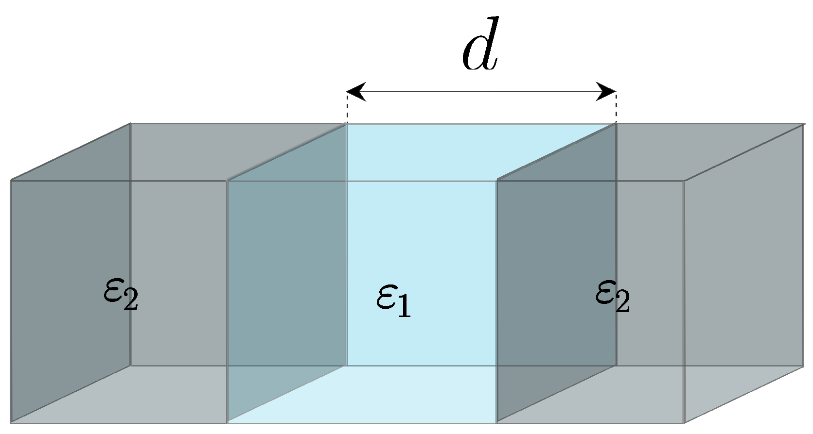
Figure 1. Sketch of the two-bulk configuration, with d the distance between the two parallel interfaces and ε 1 and ε 2 the dielectric functions for water and immersed matter.
Physics 08 00040 g001
Figure 2. Principles of the experiment reported in Ref. [51]: a silica microsphere (radius R 1 ) is held by a tightly focused laser beam close to a larger silica microsphere (radius R 2 ) that is attached to the glass slide at the bottom of the sample chamber. The distance D between the larger microsphere and the laser axis is controlled by using a piezoelectric nano-positioning system. The Brownian fluctuations of the trapped microsphere are measured for different values of D. The distance of closest approach of the two spheres is denoted d and the height of the small sphere above the glass slide h.
Physics 08 00040 g002
Figure 3. Variations in Casimir interaction energy (in units of the thermal energy k B T ) with the distance d between two dielectric microspheres in salted water for the setup depicted in Figure 2. Experimental points are shown with their error bars (blue dots)). The old approach relying on overlooking the universal contribution (red curve) leads to way too small values to be compatible with the experimental data. New theory (black curve) [52,53], with the universal contribution included, agrees fairly well with experiments (with no fitting). Adapted from Ref. [51] under copyright permission from APS.
Physics 08 00040 g003
Figure 4. Geometry for two spheres (a) or two cylinders (b) immersed in salted water. R 1 and R 2 are the radii of spheres or cylinders, and d is the distance of closest approach ( ε 1 and ε 2 are defined in Figure 1).
Physics 08 00040 g004
Figure 5. Universal functions (solid black curves) showing the variations in the universal free energy versus x = d / R eff : (a) function f calculated for two spheres with equal radii and (b) function ϕ calculated for two cylinders with equal radii. Red dotted and blue dashed lines represent the proximity-force and small-size approximations that provide the asymptotic behaviors at x 1 and x 1 , respectively.
Physics 08 00040 g005
Figure 6. Dielectric functions of water (blue curve) and tetradecane (gray curve) versus imaginary frequency ξ . The vertical red dashed line represents the first nonzero Matsubara frequency ξ 1 = 2 π k B T / at ambient temperature, where the dielectric functions of water and tetradecane are nearly identical.
Physics 08 00040 g006
Figure 7. Sketch of the two-slab configurations, with d the distance between the two parallel interfaces and w the width of the slabs ( ε 1 and ε 2 are defined in Figure 1).
Physics 08 00040 g007
Figure 8. Universal (red upper line) and non-universal (blue lower curve) contributions to the Casimir binding energy for two slabs of tetradecane of thickness w = 6 nm separated by a salted water gap d. The binding energy | F | per unit area is represented in units of thermal energy k B T per μ m 2 .
Physics 08 00040 g008
Figure 9. Casimir binding free energy between actin filaments, each having a radius 3 nm and a length 15 μm. The binding free energy | F | is drawn versus the distance d (nm) between two parallel actin filaments and measured in units of k B T . In the gray-shaded zone, | F | is dominated by the thermal energy k B T . Energies above this zone are relevant for biomechanics in the cell, and they include the physiological distance ( 6 nm ) indicated by the red solid dot. Inset: schematic of two actin filaments (blue) in a two-filament bundle, with cross-linkers shown in red. Adapted from Ref. [54] under the copyright permission from IoP.
Physics 08 00040 g009
Disclaimer/Publisher’s Note: The statements, opinions and data contained in all publications are solely those of the individual author(s) and contributor(s) and not of MDPI and/or the editor(s). MDPI and/or the editor(s) disclaim responsibility for any injury to people or property resulting from any ideas, methods, instructions or products referred to in the content.