MHD Simulations of the Solar Corona to Determine the Conditions for Large Solar Flares and the Acceleration of Cosmic Rays during Them

Abstract

Solar cosmic rays (SCRs) are generated during the primordial energy release in solar flares. This explosive process takes place in the solar corona above the active region. It represents the fast release of the magnetic field energy of the current sheet, which is formed near a singular magnetic field line. Solar cosmic rays appear as a result of the acceleration of charged particles, mainly protons, by an inductive electric field in the current sheet equal to the field E = V × B/c (with V the speed of plasma and B the magnetic field near the current sheet, and c the speed of light). To study the mechanism of solar flares and obtain conditions for studying SCR acceleration, it is necessary to carry out magnetohydrodynamic (MHD) simulations of flare situations in the solar corona above a real active region. Methods of stabilization were developed which made it possible to partially solve the problem of numerical instabilities. MHD simulations shows complicated configurations near the singular line. Comparison of the results of the MHD simulations with observations showed the general agreement of the positions of the current sheets with regions of intense flare radiation. However, there are some problems with the details of such coincidences. The results obtained in this paper show the possibility of improving the methods of MHD simulation in order to solve the problems that arise during solving of MHD equations.

1. Introduction

Solar cosmic rays are generated during the primordial energy release in solar flares. This explosive process takes place in the solar corona above the active region at altitudes of 15,000 to 70,000 km (~1/40–1/10 of the solar radius). This has been proven by direct measurements of the thermal X-ray emission of flares on the limb [1]. There are other sources of evidence for the energy release of a flare in the corona based on the analysis of observations (see, e.g., [2,3]). The possible positions of the flares found from the results of numerical simulations of the corona above the active region confirm the appearance of flares at these altitudes.

The slow accumulation of magnetic energy that occurs in the solar corona and then the energy fast release during a flare is explained by the mechanism according to which, during a flare, the energy accumulated in the magnetic field of the current sheet is released [4,5]. The current sheet, which is formed in the vicinity of a singular line of the X-type magnetic field as a result of the accumulation of disturbances, is first in a stable state. Further, in the process of quasi-stationary evolution, during which the plasma flows quickly out of the sheet under the action of the magnetic tension force, the current sheet transfers into an unstable state. The instability in the current sheet causes a flare release of energy with all the observed manifestations, which are explained by the electrodynamic model of the flare proposed by I.M. Podgorny in Ref. [6]. The model was developed based on the results of observations and numerical magnetohydrodynamics (MHD) simulations and uses analogies with the substorm electrodynamic model proposed earlier by its author [7].

Solar cosmic rays appear as a result of the acceleration of charged particles, mainly protons, by an inductive electric field in the current sheet equal to the field E = −V × B/c (with V the speed of plasma and B the magnetic field near the current sheet, and c the speed of light) [8]. This inductive electric field is caused by a rapid change in the magnetic field during current sheet instability. A similar mechanism accelerates charged particles in the pinch [9] created in an installation for solving the problem of controlled thermonuclear fusion, in spite of the fact that the magnetic field configurations in the current sheet and in the pinch are different. I.M. Podgorny noted in Refs. [8,9] an important property of this electric field which allows for clear understanding of the mechanism of cosmic ray acceleration. Both in the case of the current sheet and in the case of a pinch, charged particles are accelerated by an inductive electric field which is equal to E = −V × B/c near the main current. For solar flares, these particles (mainly protons), under favorable conditions, can leave the magnetic field above the active region, which will lead to the appearance of solar cosmic rays (SCRs).

This mechanism can accelerate galactic cosmic rays during super flares on stars to energies five orders of magnitude higher than the SCR energy [10].

In Ref. [11], an analytical solution for the current sheet was obtained and the acceleration of particles when they move in electric and magnetic fields was considered, the latter being derived from the obtained analytical solution.

To study the mechanism of solar flares, the process of the formation of a current sheet and the accumulation of energy in its magnetic field for each specific flare and to create the possibility of improving the prognosis of solar flares based on an understanding of their physical mechanism, it is necessary to carry out an MHD simulation of a flare situation in the solar corona above a real active region. The electric and magnetic fields obtained by MHD simulation above a real active region at the site of the primordial flare energy release and near it are necessary for studying the generation of solar cosmic rays. The acceleration of charged particles and the possibility of particles exit from the acceleration region to be studied by calculating the trajectories of charged particles in electric and magnetic fields obtained by MHD simulation. The first results of studying the acceleration of charged particles were obtained by calculating trajectories in electric and magnetic fields found by MHD simulation above the active region under simplified conditions [12].

Here, an MHD simulation is performed above the real active region in order to more accurately determine the configurations of the magnetic and electric fields for studying SCR generation by calculating the trajectories of charged particles. More complex field configurations are obtained and analyzed near singular lines at the places where current sheets appear. A more detailed comparison of the MHD simulation results with observations led to some problems, the solution of which requires further development of the numerical simulation technique.

When setting the conditions for the MHD simulation, no assumptions are made about the physical mechanism of the solar flare; the boundary conditions are taken from observations. For MHD simulation in the real scale of time, a high computational speed is required, which can be achieved only with parallel computing using supercomputers. The parallelization of calculations was carried out by computational threads on graphic cards (graphic processing units, GPUs). Experience has shown that the physical mechanism of a solar flare can be studied by MHD simulation only if the calculation starts a few days before the appearance of flares, when the magnetic energy for the flare has not yet accumulated in the corona. The simulation of the problem in this setting showed the appearance of a current sheet above the active region [13]. The current sheet occurrence was demonstrated by MHD simulations performed in Refs. [14,15] in the setting of a problem similar to those considered here. The initial magnetic field above the active region was almost current-free, and no magnetic energy for the solar flare existed in the corona. The boundary conditions are taken from observations without additional horizontal motions on the photosphere. MHD simulations of the solar corona in other problem settings were performed in Refs. [15,16,17,18,19,20,21,22,23,24,25,26,27,28,29,30,31,32,33].

2. Methods of MHD Simulation

MHD simulation is carried out above the active region AR10365. The computational domain in the corona is a rectangular parallelepiped (0 ≤ x ≤ 1, 0 ≤ y ≤ 0.3, 0 ≤ z ≤ 1) (the length unit chosen was L₀ = 4 × 10¹⁰ cm). The lower boundary of the computational domain y = 0 (xz-plane) is located on the surface of the Sun (the photosphere) and contains the active region; the y-axis is directed from the Sun perpendicular to the photosphere. The x-axis is directed from East to West, and the z-axis from North to South. The three-dimensional system of MHD equations,

$$\frac{𝜕B}{𝜕t}=\mathrm{rot}(V\times B)-\frac{1}{{\mathrm{Re}}_m}\mathrm{rot}\left(\frac{{\sigma }_0}{\sigma }\mathrm{rot}B\right)-\mathrm{rot}\left({\nu }_{m\_\mathrm{Art}}\hspace{0.17em}\mathrm{rot}B\right)\hspace{0.17em},$$

(1)

$$\frac{𝜕\rho }{𝜕t}=-\mathrm{div}(V\rho ),\hspace{1em}$$

(2)

$$\frac{𝜕V}{𝜕t}=-(V,\nabla )V-\frac{\beta }{2\rho }\nabla \left(\rho T\right)-\frac{1}{\rho }\left(B\times \mathrm{rot}B\right)+\frac{1}{\mathrm{Re}\rho }\Delta V+G_{g}G+{\nu }_{\mathrm{Art}}\Delta V,\hspace{0.17em}$$

(3)

$$\begin{array}{l}\frac{𝜕T}{𝜕t}=-(V,\nabla )T-(\gamma -1)T\mathrm{div}V+(\gamma -1)\frac{2{\sigma }_0}{{\mathrm{Re}}_m\sigma {\beta }_0\rho }{\left(\mathrm{rot}B\right)}^2-(\gamma -1)G_q\rho L^{\prime }(T)+\\ \frac{\gamma -1}{\rho }\mathrm{div}\left(e_{\left|\right|}{\kappa }_{dl}(e_{\left|\right|},\nabla T)+e_{\perp 1}{\kappa }_{\perp dl}(e_{\perp 1},\nabla T)+e_{\perp 2}{\kappa }_{\perp dl}(e_{\perp 2},\nabla T)\right),\end{array}$$

(4)

is solved numerically in a dimensionless form.

A typical magnetic field strength in the active region, B₀ = 300 G, is used as the unit of the magnetic field. The units of plasma density and temperature are taken to have their typical values in the corona above the active region, n₀ = ρ₀/m_i = 10⁸ cm⁻³ and T₀ = 10⁶⁰ K, which are assumed to be initially constant (m_i = 1.67 × 10⁻²⁴ g is the ion mass, ρ₀ = 1.67 × 10⁻¹⁶ g cm⁻³ is the initial plasma mass density). The units of plasma velocity, V, and time, t, are, respectively, the Alfvén velocity and the Alfvén time, $V_0=V_A=B_0/\sqrt{4\pi {\rho }_0}$ = 0.65 × 10¹⁰ cm/s and t₀ = L₀/V₀ = 6.1 s.

In Equations (1)–(4), γ = 5/3 is the adiabatic constant; Re_m = V₀L₀/ν_m0 is the magnetic Reynolds number; ν_m0 = c²/4πσ₀ is the magnetic viscosity for the conductivity, σ₀, at the temperature T₀; σ is the conductivity, σ/σ₀ = T^3/2; β = 8πn₀kT₀/B₀² (n₀ = ρ₀/m_i, k = 1.38 × 10⁻¹⁶ erg/K is the Boltzmann constant). Re = ρ₀L₀V₀/η is the Reynolds number; η is the viscosity.

G_q = L(T₀)ρ₀t₀/T₀, L(·) is the radiation function for the ionization equilibrium of solar corona [34]. L′(T) = L(T₀T)/L(T₀) is the dimensionless radiation function. e_||, e_⊥1, e_⊥2 are the orthogonal unit vectors, that are correspondingly parallel and perpendicular to the magnetic field. κ_dl = κ/(Πκ₀) is the dimensionless thermal conductivity along the magnetic field lines; Π = ρ₀L₀V₀/κ₀ is the Peclet number; κ₀ is the thermal conductivity for the temperature, T₀; κ is the thermal conductivity, κ/κ₀ = T^5/2. κ_⊥dl = [(κκ₀⁻¹Π⁻¹)(κ_Bκ_0B⁻¹Π_B⁻¹)]/[(κκ₀⁻¹Π⁻¹) + (κ_Bκ_0B⁻¹Π_B⁻¹)] is the dimensionless thermal conductivity perpendicular to the magnetic field lines and Π_B = ρ₀L₀V₀/κ_0B is the Peclet number for the thermal conductivity across the strong magnetic field (when the cyclotron radius is much smaller than the free path length). This thermal conductivity is denoted as κ_B, and κ_0B is its value for the temperature, T₀, plasma density, ρ₀, and field, B₀; κ_B/κ_0B = ρ²B⁻²T^−1/2. G_gG is the dimensionless gravitational acceleration. The dimensional vector G of gravitational acceleration in the solar corona is directed to the Sun perpendicular to the photosphere, its absolute value is 2.74 × 10⁴ cm/s², so that in the chosen coordinate system G = (0, 2.74 × 10⁴, 0). G_g is the value which inverse to the dimensionless unit of acceleration G_g = (V₀/t₀)⁻¹ = 0.94 × 10⁻⁹ s²/cm. The gravitational acceleration of the plasma is ~10⁻⁵ dimensionless units, it is much less than the acceleration of the magnetic force and the pressure force, so it can be neglected. In most calculations, gravitational acceleration was neglected, setting G_g = 0.

To select the parameters, the principle of limited simulation [35] was used, according to which much larger and much smaller units of dimensionless parameters were set in calculations much larger and much smaller than unity without accurately preserving their values. The main parameters were the magnetic and ordinary Reynolds numbers, Re_m and Re. Dimensionless values of artificial viscosities (ν_{m_Art_Ph} and ν_{Art_Ph}) were set to stabilize the numerical instabilities.

For the numerical solution, an upwind, absolutely implicit finite-difference scheme was developed which is conservative with respect to the magnetic flux [36]. The scheme is solved by the method of iterations. The methods were applied with the aim of constructing a scheme that remains stable for the maximum possible time step. The scheme was realized in the computer program PERESVET [36].

A stable finite-difference scheme (high stability is achieved if this scheme is implicit) should approximate the magnetic induction Equation (1), in which the diffusion term is taken as ν_mΔB rather than −rot(ν_mrotB). For this purpose, it is necessary to preserve the magnetic flux through the boundary of each cell of the difference scheme, which means that the finite-difference analog [divB] is equal to zero with high accuracy if the values are correctly specified on the grid elements of the difference scheme. For a difference scheme conservative with respect to the magnetic flux, the finite-difference analogs of [ν_mΔB] and [−rot(ν_mrotB)] coincide. If, in the finite-difference scheme, the magnetic flux is conserved with high accuracy, then the scheme with finite-difference approximation of the diffusion term in the form [−rot(ν_mrotB)] is also stable, since this diffusion term is equal to [ν_mΔB] with high accuracy. In addition, when solving a finite-difference scheme by the iteration method, the values at the central point of the template can be taken both at the current iteration and at the next iteration. It becomes possible to use various variants of the difference scheme. The above considerations for the constant magnetic viscosity, ν_m, extend to the case where ν_m depends on spatial coordinates. For this, it is necessary to add finite-difference analogs of the products of the spatial derivatives of ν_m and the spatial derivatives of the B components to the scheme which do not cause instability of the difference scheme.

For the numerical solution of the MHD equations, several versions of the scheme were proposed, in which the magnetic flux was conserved with high accuracy. A more accurate visual representation of the arrangement of quantities on a three-dimensional grid of a finite-difference scheme, conservative with respect to the magnetic flux, was produced. Images of the locations of the values on the grid are shown in Figure 1 and Figure 2. The finite-difference analogue of the magnetic field divergence, [divB], for such a scheme should be equal to zero with high accuracy; for our calculations, the dimensionless value |[divB]|~10⁻⁴. In connection with the appearance of numerical instabilities near the boundary of the region, additional test calculations were carried out for possible corrections in the choice of the scheme variant with the conservation of the magnetic flux. As a result, taking into account the influence of instabilities near the boundary, the variant in which the iterations converge the fastest remains the most efficient. In this version, the diffusion term in the equation for the magnetic field was taken in the form of a finite-difference analog ΔB ([ΔB]), rather than rot(rotB) ([rot(rotB)]), and the values at the central point of the grid stencil of the finite-difference scheme were taken in the next iteration.

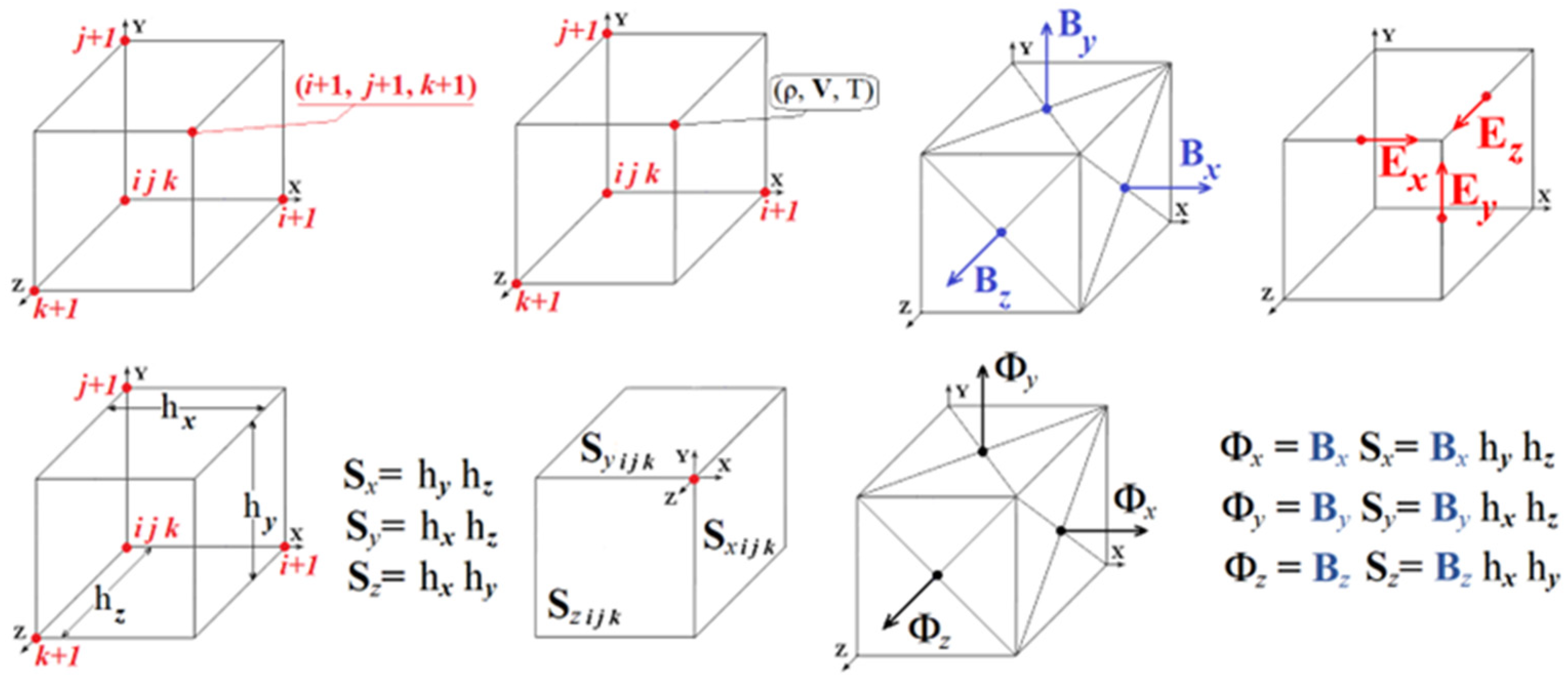
In the finite-difference scheme, which is conservative with respect to the magnetic flux, the magnetic field is specified not by the field vectors at the grid points, but by the magnetic fluxes through the boundaries of the grid cells, averaged per unit area (Figure 1). Used to specify the magnetic field components, the magnetic fluxes through the cell faces, averaged per unit area, approximate the components of the magnetic field vector perpendicular to the given face, taken at the central point of the given face. The values of plasma density, ρ, velocity, V, and temperature, T, were set at the grid points of the finite-difference scheme, i.e., at the vertices of the cubes, which are grid cells.

The dimensionless electric field E = −V × B + ν_mj (here, ν_m = Rm⁻¹ (σ₀/σ) = Rm⁻¹T^−3/2 is the dimensionless magnetic viscosity) and the dimensionless electric current density j = rotB are not included in the equations of magnetic hydrodynamics but are expressed in terms of the quantities included in these equations. It is convenient to use the variables E and j for constructing a difference scheme; their values are determined at the edges of the grid cells. The edges of the grid cells, which can be parallel to one of the coordinate axes x, y or z are numbered by the Latin letters i, j, k (in the three dimensional space) of the end of this edge with the minimum value of the corresponding coordinate.

The magnetic field Equation (1) in the introduced notation has the form $\frac{𝜕B}{𝜕t}=\mathrm{rot}(-E)$. The flux of the magnetic field, B, through the surface of a small area, S, perpendicular to the vector, B, is equal to Φ_B= B S (if there is an arbitrary surface of a large area, then the magnetic flux through it can no longer be expressed through the field vector at any one point; the magnetic flux will be equal to the integral over the surface, ${\mathsf{\Phi }}_{\mathrm{B}}={\displaystyle \underset{S}{\iint }({\rm B},ds)}$, where B is the magnetic field vector defined at each point of the surface; ds is the vector perpendicular to the surface, the value of which is equal to the small area, ds, on the surface under consideration; and (B,ds) is the scalar product of these vectors).

The flux of the vector rot(−E) through the surface of a small area, S, perpendicular to the vector rot(−E) is equal to Φ_rot(−E) = rot(−E) S. According to the induction equation $\frac{𝜕B}{𝜕t}=\mathrm{rot}(-E)$, this flow, Φ_rot(−E), represents a change in time of the magnetic flux, Φ_B. Since the divergence of the magnetic field must always be zero: divB = 0, the magnetic flux through a surface bounding any region in space will be zero. This confirms the induction equation, from which it follows that, if, for an initial magnetic field, its flux through the surface bounding any region in space is zero, it will remain zero for any moment in time, since the flux of the vector field rotor (in this case, rot(−E)), representing the change in time of the magnetic flux, is always zero.

To improve stability, a scheme was constructed in which the flow through the grid cell boundary remains equal to zero with high accuracy (with the accuracy of iteration convergence if this is an implicit scheme solved by the iteration method or with the accuracy of representing numbers in a computer if an explicit scheme is used, which is less stable). This is a scheme that is conservative with respect to magnetic flux.

The magnetic flux through a face perpendicular to the x-axis is equal to the product of the magnetic field component, B_x, defined for this face by the area of this face.

Φ_x,i,j,k = B_x,i,j,kS_x = B_x,i,j,kh_yh_z (h_y, h_e are the grid steps along the y and z axes; see Figure 1, bottom).

Similarly, magnetic fluxes are determined through faces perpendicular to the y and z axes. The total flux of the magnetic field emerging through the surface limiting the volume of the computational grid cell with the numbers i + 1, j + 1 and k + 1 (the cell shown in Figure 1 with the limits of coordinate change (x_i ≤ x ≤ x_i+1, y_j ≤ y ≤ y_j+1 and z_k ≤ z ≤ z_k+1)) can be found by determining the flows through the faces of this cell; for a scheme that is conservative with respect to the magnetic flux, this value should be equal to zero (with high accuracy):

Φ_{x,i+1,j+1,k+1} − Φ_x,i,j+1,k+1 + Φ_{y,i+1,j+1,k+1} − Φ_y,i+1,j,k+1 + Φ_{z,i+1,j+1,k+1} − Φ_z,i+1,j+1,k = 0,

or, substituting the values of magnetic fluxes:

B_{x,i+1,j+1,k+1}S_x – B_x,I,j+1,k+1S_x + B_{y,i+1,j+1,k+1} S_y − B_y,i+1,j,k+1 S_y + B_{z,i+1,j+1,k+1}S_z − B_z,i+1,j+1,kS_z = 0,

where S_x, S_y and S_z are the areas of cell faces perpendicular to the vectors of the selected coordinate system, e_x e_y e_z : S_x= h_yh_z, S_y= h_xh_z and S_z= h_xh_y.

The density of the magnetic flux source in a grid cell is the value of the total magnetic flux divided by the volume of the cell. Dividing the total magnetic flux by the volume, V = h_xh_yh_z, of the grid cell, one obtains:

(B_{x,i+1,j+1,k+1} − B_x,i,j+1,k+1)/h_x + (B_{y,i+1,j+1,k+1} − B_y,i+1,j,k+1)/h_y + (B_{z,i+1,j+1,k+1} − B_z,i+1,j+1,k)/h_z= 0,

i.e., the finite-difference analog of the magnetic field divergence, divB ([divB]), vanishes, as expected.

Equality to zero of the total flux of the magnetic field through the cell boundary in a scheme that is conservative with respect to the magnetic flux is achieved by setting the initial magnetic field on the faces of the grid cells with zero total magnetic flux and zero change in the flux with time. The change in the magnetic flux, representing the flux of the vector rot(−E), which goes through the boundary of the grid cell, will be zero if, in the scheme, the components of the vector rot(−E), the finite-difference analogs of the derivatives, are expressed in terms of the components of the vectors, the electric field, E, specified on the edges of the cells grids, as illustrated in Figure 2.

Despite the use of special methods, simulation in real time is possible only with the help of parallel computing. The simulations were carried out by means of parallel computing threads on graphics cards using CUDA (Compute Unified Device Architecture) technology described in Ref. [37].

The main problem in MHD simulation above a real active region is the numerical instabilities that arise near the boundary of the computational region. The developed methods for stabilizing the instability made it possible to partially solve the problem for calculations with relatively low viscosities (Re_m = 10⁹, Re = 10⁷), which practically do not suppress the perturbation propagating from the photosphere. The results obtained make it possible to determine ways to further improve the technique for stabilizing numerical instabilities.

3. Results

Current sheets exist for a long time before a flare, causing pre-flare radiation, which can be used to determine the position of the current sheet. When instability of the current sheet occurs during a flare, the energy of the magnetic field of the current sheet is rapidly released, the plasma is rapidly heated, the radiation increases sharply in all ranges and protons are accelerated at energies of up to 20 GeV. This behavior of the current sheets was confirmed by our comparison of the MHD simulation results with observations three hours before the flare and during the flare.

A number of electrons accelerate during a flare, and electrons heated during the flare and pre-flare release of magnetic energy in the current sheets to temperatures of several tens of millions of degrees, which produce radio emissions at a frequency of 17 GHz, do not propagate far from the site of the primordial energy release of the flare. This is evidenced by the compactness of the radiation source at a given frequency, as well as the general coincidence of the positions of the current sheets obtained as a result of MHD simulations with regions of intense flare radiation. Therefore, the source of radio emission measured at a frequency of 17 GHz by the Nobeyama radioheliograph was used to determine the location of the primordial energy release of the flare.

MHD simulations above AR10365 were carried out for 3 days from 24 May 2003 20:47:59 to 27 May 2003 20:47:59. The results of further simulations after 27 May 2003 20:47:59 could be of greater interest since the most powerful flares appeared then. However, further simulations were not carried out, as difficulties arise in setting the conditions on the photospheric boundary due to its position at a small angle to the line-of-sight direction when the active region is located near the boundary of the solar disk.

The configuration of the magnetic field obtained by MHD simulation is so complex that it is often impossible to determine from this configuration the positions of singular lines and the current sheets appearing near them from it. For this purpose, a graphical search system of flare positions has been developed [13] and modernized. The system is based on the search for current density maxima, which are reached in the middle of the current sheets, and further analysis of the magnetic field configuration near the points of the found maxima.

The results presented here are a continuation of the study reported in Ref. [38], where the MHD simulations above AR10365 were carried out for time interval on 25 May 2003 at relatively high viscosities (Re_m = 3 × 10⁴, Re = 10⁴) and in Ref. [39], which presents a comparison of the results of MHD simulations above AR10365 with observations made on 27 May 2003 at 02:43. The conclusions presented here were reached on the basis of a generalization of both these results and the results obtained in this work.

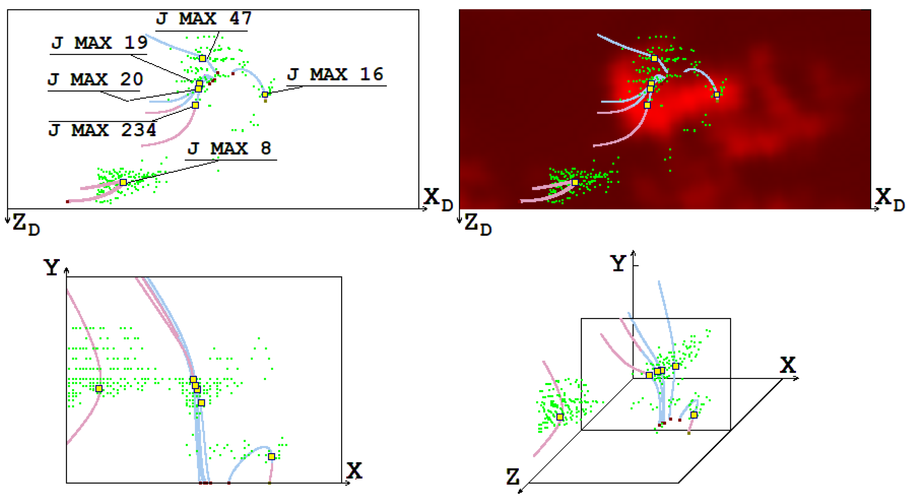
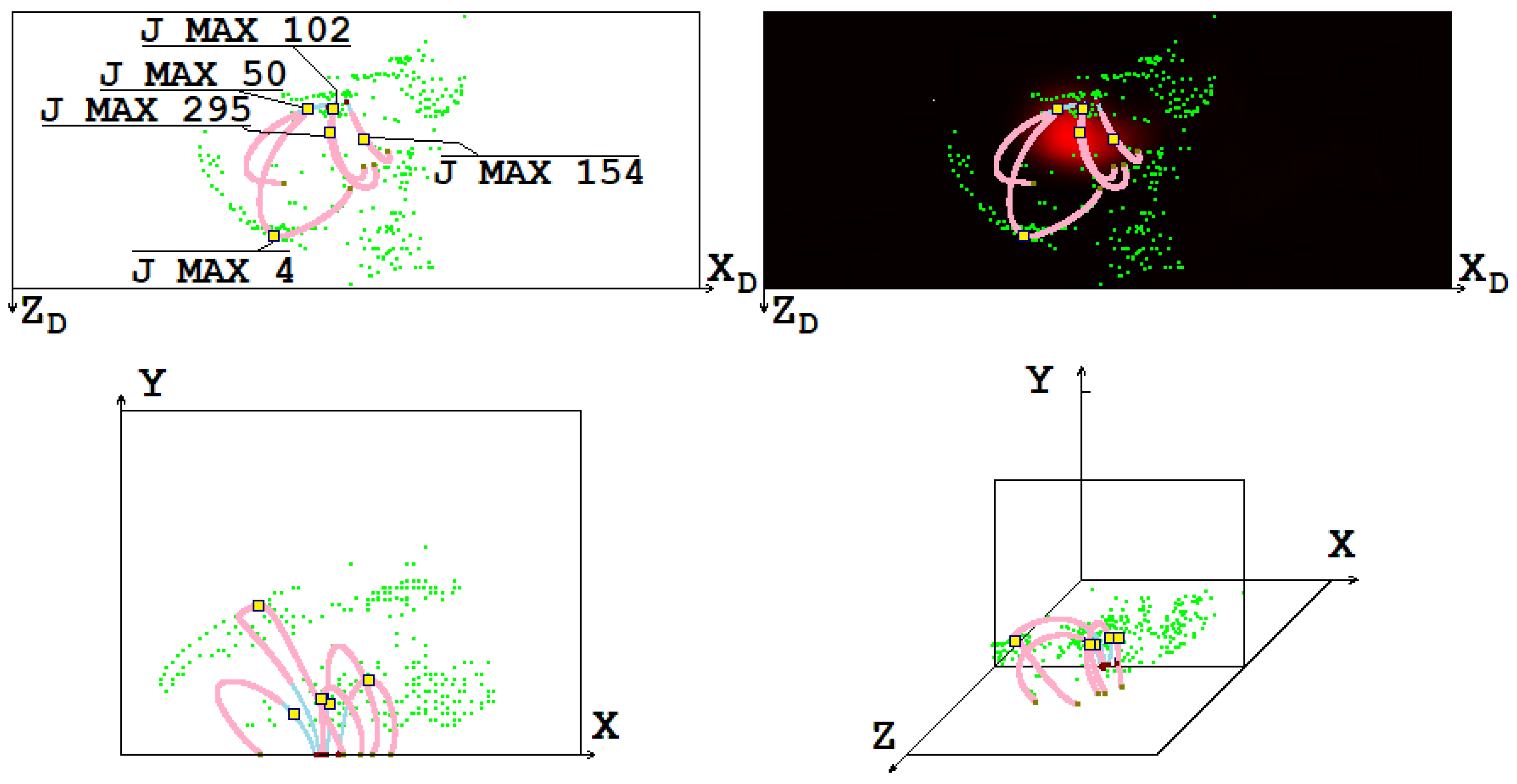
Figure 3 and Figure 4 present a comparison of the results of MHD simulations with observations of radio emissions at a frequency of 17 GHz obtained with the Nobeyama Radioheliograph (NoRH [40]) before the M1.9 flare on 26 May 2003 above the active region of AR10365 and during this flare (26 May 2003, 02:32:05 and 05:50:03). The positions of the selected current density maxima with numbers 8, 16, 19, 20, 47 and 234 at 02:32:05 and 4, 50, 102, 154 and 295 at 05:50:03 are marked, and the remaining maxima are indicated by green dots (the current density maxima are numbered in decreasing order of density current). The configuration of the magnetic field is represented by magnetic lines passing through these selected current density maxima. Magnetic lines in a three-dimensional space of the computational domain in the solar corona above the active region AR10365, projections of magnetic lines onto the central plane of the computational domain (z = 0.5) (this central plane is perpendicular to the solar surface and parallel to the solar equator), and projections of magnetic lines onto the picture plane, which is perpendicular to the line of sight, are shown. The projections of magnetic lines onto the picture plane are also plotted together with the intensity distributions of radio emissions at a frequency of 17 GHz obtained using NoRH in order to compare the results of the MHD simulations with observational data.

As was mentioned at the beginning of Section 2, the computational domain is a rectangular parallelepiped with edges directed along the axes of the selected coordinate system, X, Y, Z. The Y-axis is directed from the Sun perpendicular to the solar surface, the X-axis is directed from East to West, and the Z-axis from North to South. The lower boundary of the computational domain (YZ) is located on the solar surface and contains the active region. In Figure 3 (upper) and Figure 4 (upper), the vertical and horizontal coordinates on the solar disk, X_D and Z_D, are indicated. The X_D-axis is directed from left to right, the Z_D-axis from top to bottom. The Y_D-axis is directed along the line-of-sight from the Sun. The X_D, Y_D, Z_D coordinates are closest to the chosen coordinates of the computational domain. When the active region is located in the center of the solar disk and at zero inclination of the axis of rotation of the Sun, B_0, the coordinate axes X, Y, Z and X_D, Y_D, Z_D coincide. At the selected moments, the solar tilt angle, B_0, is ~1.5 degrees and the position of the active region is approximately S07W02, so the angles of inclination of the X_D- to X-, Y_D- to Y-, and Z_D- to Z-axes are no more than 10 degrees.

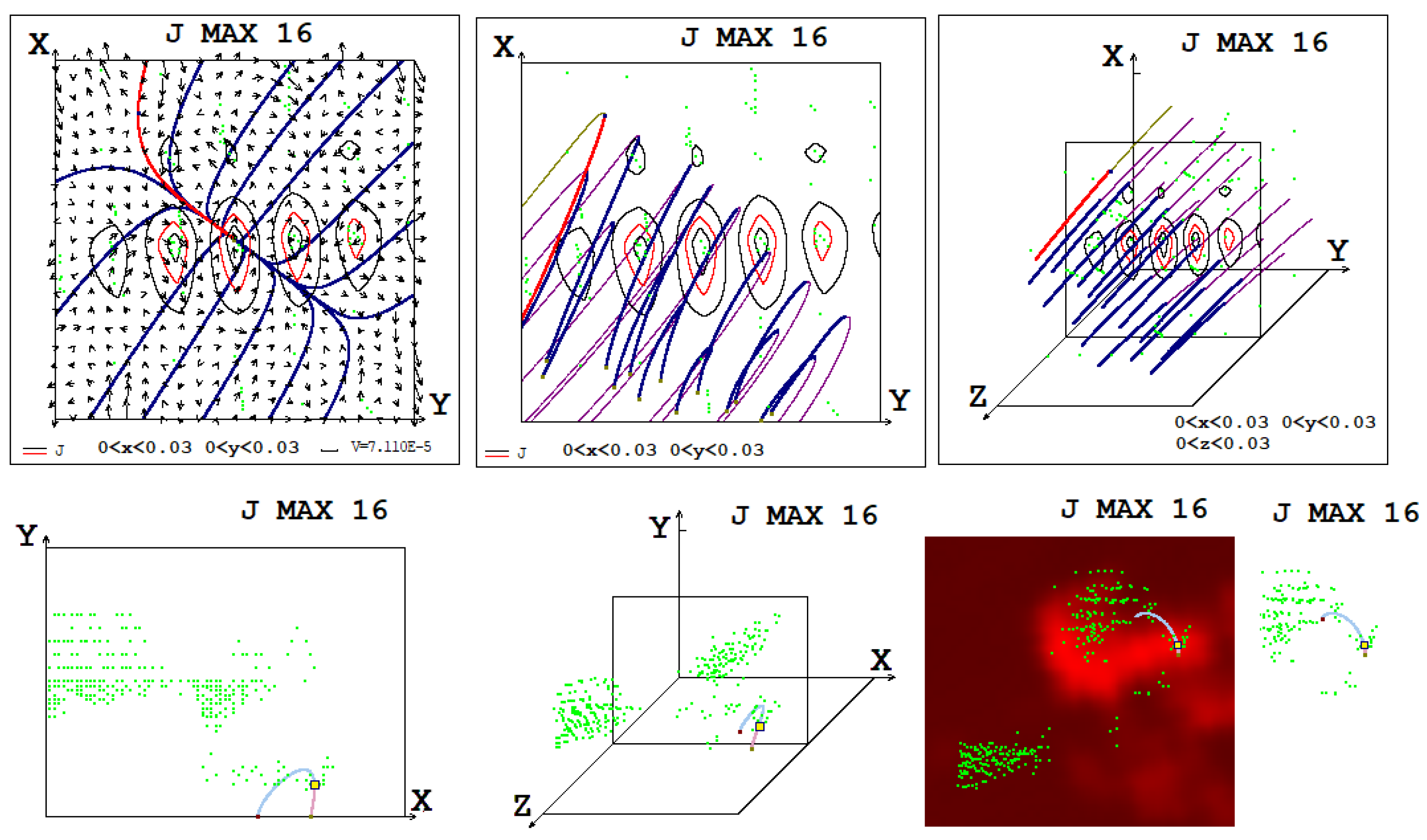
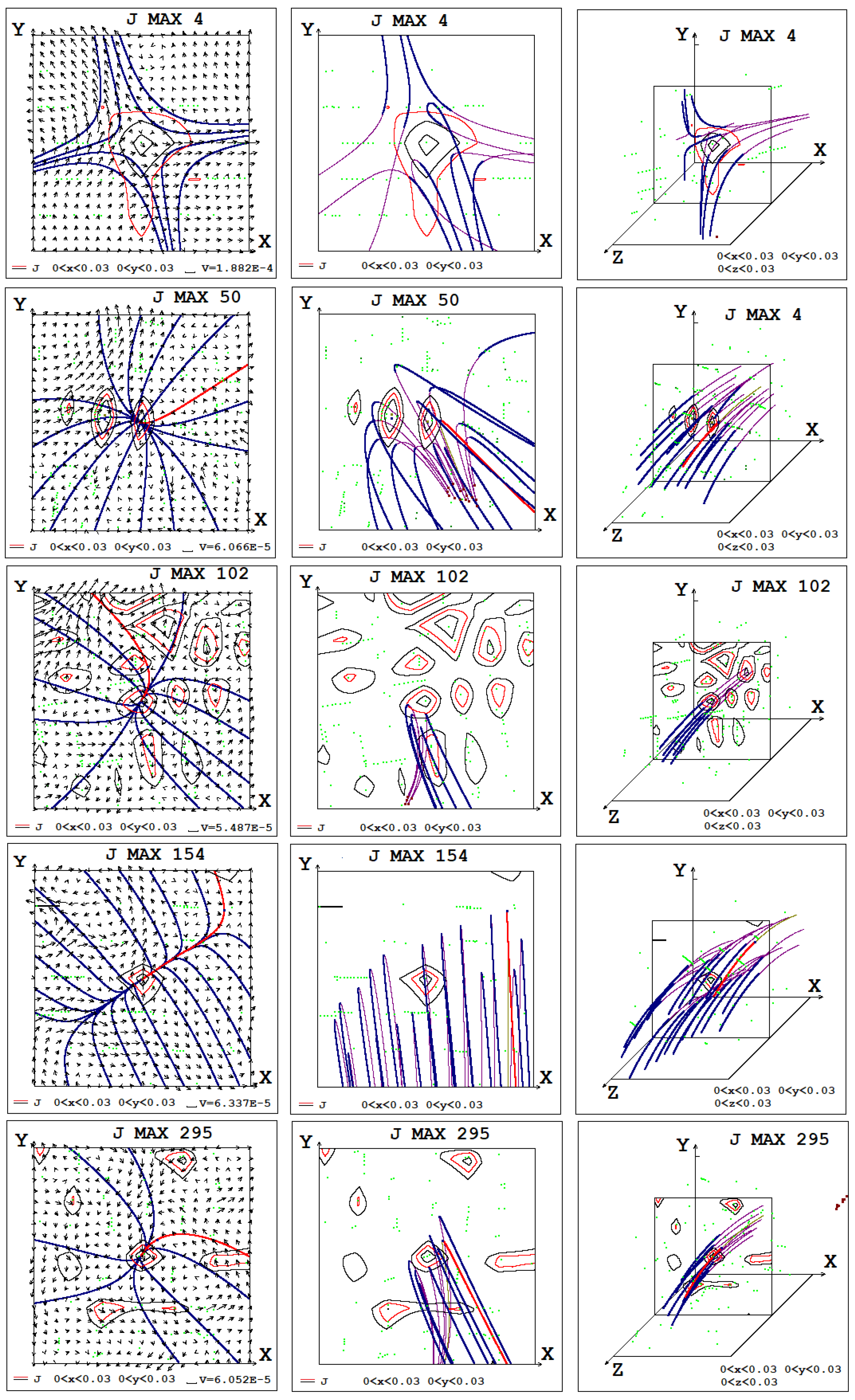
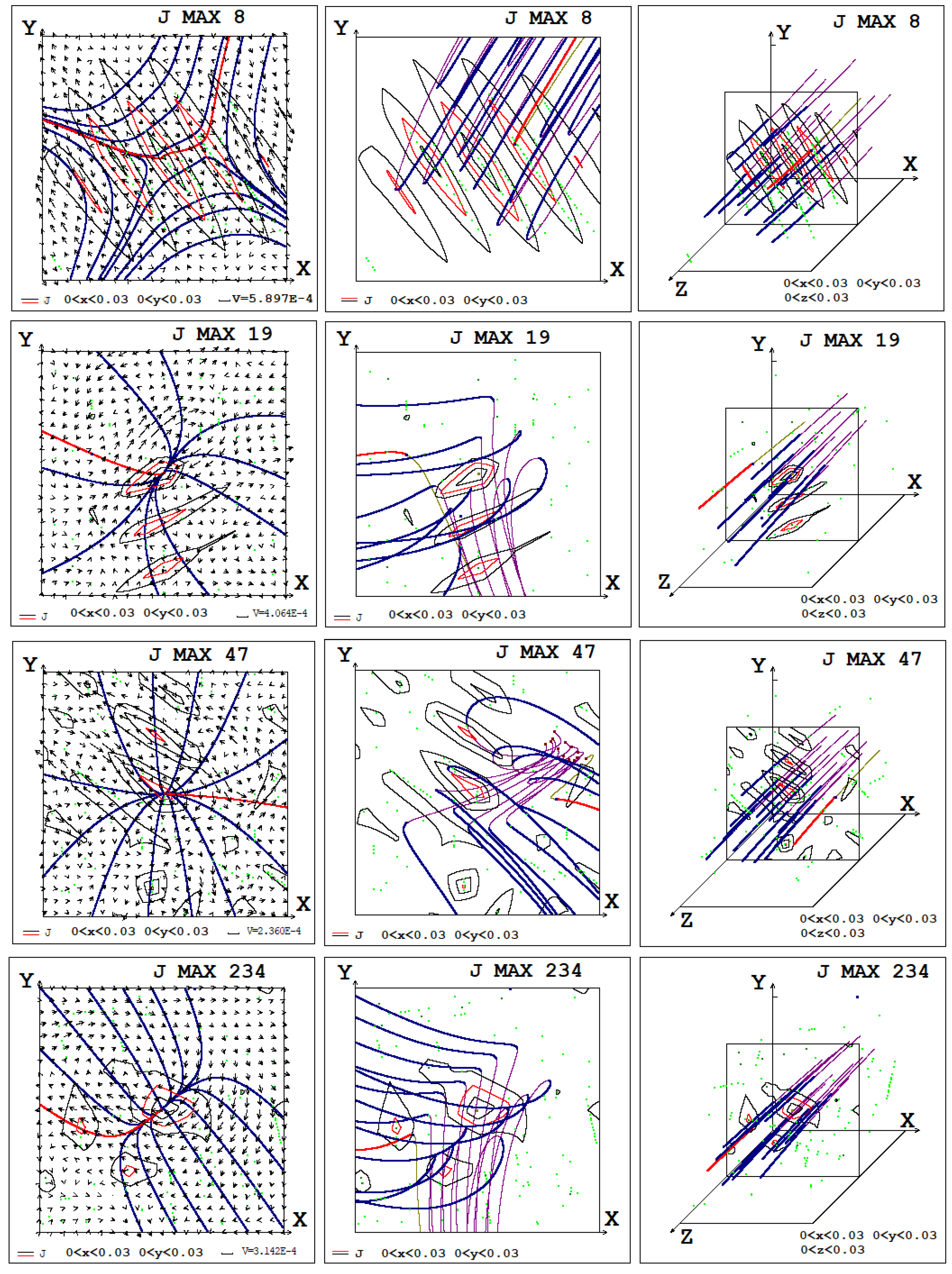
The magnetic field configurations near the current density maxima, which to be situated on singular magnetic lines and which are places of magnetic energy accumulation for solar flare, are shown in Figure 5 for the 8th, 19th, 47th and 234th maxima and in Figure 6 for the 16th maximum, which were chosen as examples. These configurations show that a divergent magnetic field is superimposed on the X-type magnetic field at many current density maxima. In view of some insignificant differences between the configurations near the 19th and 20th maxima, Figure 5 shows only the configuration near the 19th maximum. The 16th maximum of the current density, located on the solar disk in the region of radiation at a frequency of 17 GHz of sufficiently high intensity, is of interest since it has a number of properties that increase the probability of the accumulation and rapid release of flare energy for this current sheet. The 16th maximum is located near the top of the loop and has a rather powerful X-type configuration (Figure 6). The divergent field dominates just weakly and has almost the same effect as the X-type field, as can be seen from the configuration of lines tangential to the projections of the magnetic field vectors onto the plane of the current sheet configuration (the location of the plane of the current sheet configuration is explained in Figure 5 captions).

In general, the divergent magnetic field causes the rotational motion of plasma around the singular line, which interferes with current sheet creation to accumulate the magnetic energy for solar flare. However, due to the presence of the X-type configuration, current sheets are formed at such locations even if the divergent field dominates and a deformed divergent magnetic field is obtained as a result of the superposition.

The simulation shows that, for a rather large number of current density maxima, the longitudinal component of the magnetic field is large, so that the 3-dimensional magnetic field lines are almost parallel. For such singular magnetic lines, the pressure of the longitudinal magnetic field can stabilize the current sheet and in such a way to interfere with the fast energy release. But it is impossible to say that a flare in such a situation cannot occur because the appearance of instability is defined not only by the pressure of the longitudinal magnetic field, but also by a number of factors and it is quite a complicated task to estimate their mutual influence. Also, the simulation shows the positions of some current density maxima near the tops of magnetic loops, but the large number of maxima are situated far from the tops of the magnetic loops, where the magnetic field is directed almost vertically.

4. Discussion

In this paper, a comparison of the results of MHD simulations with observations before and during flares showed a general agreement between the positions of the current sheets found by our graphical search system and the regions of intense flare radiation. A significant number of points at which current density maxima were found are located in the region of strong radiation. Also, a significant number of the points of maxima were found are located at relatively small distances from the region of strong radiation (~10 Mm and less), which can be explained by the error of the numerical method and the physical processes during the flare. These results confirm the mechanism according to which the energy accumulated in the magnetic field of the current sheet is released during a flare.

There are some problems with the details of such coincidences. The problems arise especially if you choose current sheets in which the current directions are almost parallel to the solar surface and are located at the tops of magnetic loops (or at least near the tops of magnetic loops) at a fairly high altitude of 25,000–45,000 km. These heights are lower than 60,000–70,000 km, where it is difficult to expect the accumulation of large magnetic energy due to low magnetic fields, but at the same time these are not heights of 15,000–20,000 km, where, apparently, a current sheet may not appear with a sufficiently small longitudinal field so that explosive instability can occur in it. In the magnetic field of current sheets at the tops of magnetic loops at altitudes of 25,000–45,000 km, apparently, energy for a flare can accumulate best of all, and after a quasi-stationary evolution such current sheets can go into an unstable state.

The results obtained indicate the need for the further work to solve the problems that have arisen. In spite of the large number of current density maxima in the bright region of intensive flare emission or near it, also, there are a large number of current density maxima situated far from the bright region (at distances of about 20 Mm, 30 Mm and more). Moreover, the current density maxima which are the most probable candidates for the solar flare positions are situated out of the bright region. Such a current density maximum is the maximum number 4 (see Figure 4 and Figure 7), situated at a distance of more than 20 Mm from the bright region. The X-type magnetic field is dominated in the magnetic field configuration near the singular line on which the fourth current density maximum is situated. The longitudinal magnetic field component is not much larger than its component in the plane of configuration (the field of the X-type configuration and the field of current along the singular line); this can be concluded from the observation that the magnetic lines near the singular line are not parallel (Figure 7). The fourth current density maximum is situated near the top of the magnetic loop.

Certainly, the physical processes near the singular lines and in the current sheets can be more complicated. It may be that near the current density maxima, which, according to our MHD simulation, are situated in the bright region of intensive flare emission, there is effective magnetic energy accumulation followed by the appearance of instability with strong flare energy release.

Also, it is possible that current density maxima such as the fourth maximum were not situated in the bright region of intensive flare emission because our MHD simulation was not sufficiently precise. The solutions of MHD equations can be distorted by disturbances propagated from the places of numerical instability near the boundary of the computational domain. Simulations can have insufficient precision due to rather large space steps in the numerical grid. Also, the solutions of MHD equations can be distorted as a result of not setting sufficiently accurate conditions for the magnetic field on the solar surface boundary. To understand the real reason why such types of current density maxima are situated in the bright region is a problem which it is necessary to solve.

It is necessary to carry out more accurate calculations. This can be helped by a more efficient stabilization of the instability near the boundary of the computational domain as well as by a more accurate setting of the boundary conditions, which is possible now. The obtained results show the way to modernize numerical methods to perform more precise simulations which can be used to solve the problems that have appeared.

5. Conclusions

The following conclusions are in order.

• The methods of MHD simulation of the solar corona above a real active region have been improved. The application of these methods made it possible to perform calculations above the active region AR10365 during a time interval of about three days but showed the need for further modernization. For the upwind, absolutely implicit finite-difference scheme which is conservative with respect to the magnetic flux that was developed and implemented using the PERESVET program, a variant of magnetic flux conservation was chosen for which the stabilization of the numerical instability that occurs near the boundary of the computational domain is best performed. The parallel computing algorithm implemented by computational threads on graphics cards using CUDA technology has been modernized over the past few years since its first version was developed. The stabilization of the numerical instability that occurs near the boundary of the computational domain has been improved by more accurate selection of artificial viscosity values and by using other methods.
• An analysis of the new results of MHD simulation before solar flares and during solar flares confirmed the formation of singular X-type lines in the magnetic field configuration and the appearance of current sheets in them, in the magnetic field of which energy for solar flares is accumulated.
• The results obtained confirmed the existence of a large number of singular magnetic field lines, in the vicinity of which a divergent magnetic field is superimposed on the X-type field configuration. Even if the divergent magnetic field dominates, such that a deformed divergent magnetic field results from the superposition, the presence of an X-type field can produce a sufficiently strong current sheet to explain the appearance of a medium-power flare.
• The results of the analysis of MHD simulation data for the time moments before and during flares confirmed that a large number of current density maxima (more than a hundred), located on a singular magnetic field line in the vicinity of which the current sheet is formed, are in the region of intense flare radio emission at a frequency of 17 GHz or at a distance from the region of intense radiation not exceeding 10 Mm. This arrangement of current density maxima confirms the solar flare mechanism based on the release of energy stored in the magnetic field of the current sheet. The details of the location of the current density maxima did not always correspond to the observational data, which indicates the need to develop more accurate methods for solving the equations of magnetohydrodynamics and setting the boundary conditions on the solar surface.