Enhancing Temperature Data Quality for Agricultural Decision-Making with Emphasis to Evapotranspiration Calculation: A Robust Framework Integrating Dynamic Time Warping, Fuzzy Logic, and Machine Learning

Abstract

This study introduces a comprehensive framework for assessing and enhancing the quality of hourly temperature data collected from a six-station agrometeorological network in the Arta plain, Epirus, Greece, spanning the period 2015–2023. By combining traditional quality control (QC) techniques with advanced methods—Dynamic Time Warping (DTW), Fuzzy Logic, and XGBoost machine learning—the framework effectively identifies anomalies and reconstructs missing or erroneous temperature values. The DTW–Fuzzy Logic approach reliably detected spatial inconsistencies, while the machine learning reconstruction achieved low root mean squared error (RMSE) values (0.40–0.66 °C), ensuring the high fidelity of the corrected dataset. A Data Quality Index (DQI) was developed to quantify improvements in both completeness and accuracy, providing a transparent and standardized metric for end users. The enhanced temperature data significantly improve the reliability of inputs for applications such as evapotranspiration (ET) estimation and agricultural decision support systems (DSS). Designed to be scalable and automated, the proposed framework ensures robust Internal Consistency across the network—even when stations are intermittently offline—yielding direct benefits for irrigation water management, as well as broader agrometeorological applications.

1. Introduction

Accurate and reliable temperature measurements are essential for various environmental and agricultural applications, including climate monitoring, crop management, irrigation water management, etc. However, ensuring the quality of temperature data collected from automated weather station networks remains a major challenge, as measurement time series are often affected by sensor malfunctions, missing values, and spatial inconsistencies. Without proper quality control, erroneous or incomplete temperature data can lead to the incorrect modeling of agricultural processes and hence negatively affect productivity. Therefore, it is critical to implement a robust data quality framework to enhance user confidence in the reliability of these measurements [1].

Traditional quality control (QC) methods, such as Gross Error Limits, Step Tests, and persistence checks, provide an initial validation, but often fail to detect contextual outliers [2,3]—temperature values that appear reasonable in isolation, but deviate from expected spatial or temporal trends. Additionally, existing QC approaches do not adequately address long-term missing values, which occur when a weather station is offline for an extended period.

Despite the utility of traditional quality control methods like gross error limits, Step Tests, and persistence checks, these techniques exhibit several limitations. They primarily focus on identifying obvious anomalies without adequately capturing contextual or spatial inconsistencies, especially when errors appear reasonable in isolation. Furthermore, they often lack the mechanisms to deal with extended periods of missing data, introducing gaps that can compromise model reliability. Spatial Consistency Tests, while promising, are sensitive to missing values and seasonal variations, reducing their effectiveness in automated pipelines. These challenges underscore the need for a more robust framework that not only enhances data completeness and accuracy, but also ensures spatial coherence across networks. Recent studies [4] demonstrate the value of integrating quality control with automated gap-filling to ensure continuous, usable temperature datasets. In this work, by integrating Dynamic Time Warping (DTW), Fuzzy Logic, and machine learning-based reconstruction, we address these limitations, offering an innovative and practical solution for the comprehensive assessment and improvement of temperature data quality.

To overcome these challenges, advanced techniques such as Dynamic Time Warping (DTW) and Fuzzy Logic can improve anomaly detection, while Machine Learning (ML) models can reconstruct missing temperature values with high accuracy. Boujoudar et al. [5] recently compared several ML algorithms for meteorological time series reconstruction, with XGBoost and similar ensemble methods showing strong accuracy and adaptability to nonlinear patterns. This study aims to establish a trustworthy temperature data quality framework by performing the following:

• Implementing a Spatial Consistency Test using Dynamic Time Warping (DTW) and Fuzzy Logic to detect anomalies in temperature measurements.
• Applying ML-based reconstruction (using XGBoost) to fill missing values while preserving seasonal and spatial temperature patterns.
• Developing a Data Quality Index (DQI) to quantify the overall reliability of temperature measurements, ensuring transparency and usability for water management and agricultural applications.

By integrating these approaches, we provide a systematic data quality assessment that enhances trust in temperature data. This work ensures that end users (including farmers, agriculturalists, irrigation consultants, and researchers) can confidently utilize temperature data for evapotranspiration modeling, DDS (Decision Support Systems)-based irrigation scheduling, climate studies, etc. The main body of this paper is structured as follows: Section 2 describes the weather station network and temperature dataset. Section 3 details the methodology, including QC tests, anomaly detection, and ML-based reconstruction. Section 4 presents the results of the quality assessment. Section 5 discusses the findings and their implications for real-world applications.

2. Temperature Dataset Characteristics and Data Quality Challenges

2.1. Temperature Time Series and Types of Observed Errors

The temperature time series analyzed in this study originates from UOI-DAGRI weather station network (Figure 1) (

Table 1. Coordinates and altitude of UOI-DAGRI weather station network.

	Uoi	Big	Ag	Neo	Kom	Kam
Latitude (°)	39.12208	39.07888	39.14904	39.05061	39.09518	39.21634
Longitude (°)	20.94737	20.88525	20.87591	21.01207	21.06071	20.91295
Altitude (m)	10	0	10	10	15	20

), covering the period from 2015 to 2023. Temperatures were logged every 10 min, and those measurements have been aggregated into 1 h intervals for the present analysis. In meteorological data collection, errors can generally be classified into random errors and systematic errors [6]. Random errors are unpredictable fluctuations that arise from temporary environmental influences, sensor noise, or small variations in measurement conditions. These errors tend to cancel out when averaging multiple observations. In contrast, systematic errors are consistent biases introduced by calibration issues, sensor degradation, or improper placement of instruments. Unlike random errors, systematic errors do not diminish with repeated measurements and require identification and correction using calibration or algorithmic adjustments. Understanding these error types is crucial for ensuring the reliability of temperature measurements.

For the UOI-DAGRI weather station network, one of the most common and evident issues in the dataset is the presence of missing values (NaN). These missing periods can occur sporadically for individual time steps or extend over longer durations (e.g., months), typically due to a station being out of service. However, there no long periods of missing data overlapping across the network. In cases where a station experienced data loss, at least five out of the six stations remained operational. Nevertheless, there were instances when up to three stations simultaneously recorded missing values for a short period of time.

Another type of systematic error involves extreme erroneous values that lack physical plausibility. Occasionally, temperatures exceeding 100 °C or dropping below −20 °C were observed in the raw time series. These errors are infrequent and easily identifiable using visual inspection. Their causes cannot always be determined with certainty, but may stem from statistical malfunctions of electronic components, such as analog-to-digital converter (ADC) overflow or unexpected system reboots.

A more subtle but problematic systematic error type involved periodic erroneous temperature values. In some cases, one out of every four measurements exhibited deviations, albeit within a plausible range. This pattern was attributed to a malfunctioning temperature sensor and persisted until the sensor was replaced during maintenance. This type of error is particularly challenging to detect, as it does not always trigger automated alarms and can persist for weeks without being visually apparent.

Another notable issue was observed where, for certain days, the recorded temperatures appeared to follow the general trend of the other stations, but only above a specific threshold. This anomalous behavior ceased after maintenance, suggesting a station-specific malfunction. Finally, comparing the temperature values of a station with those of the neighboring stations, contextual outliers can create anomalies that may appear normal when viewed in isolation, but which are considered outliers when analyzed within their specific temporal or spatial context. In temperature data, these anomalies occur when a measurement deviates significantly from the expected values based on time of day, season, or surrounding stations. For example, a temperature reading of 15 °C at 3:00 AM during the winter might be considered an outlier if the surrounding stations report temperatures close to 5 °C. However, the same 15 °C reading in the afternoon might be entirely normal, demonstrating the importance of considering the temporal and spatial contexts in anomaly detection.

Overall, the temperature data from the weather station network can be considered reliable, with some short- and long-term missing values and occasional erroneous measurements arising due to sensor malfunctions. No time shift errors were found in the time series. Raw data from the network measurements can be accessed at: https://dagri.uoi.gr/atoo/ (accessed on 29 March 2025).

2.2. Challenges of Network Operation and Data Analysis

In addition to the data-specific challenges described above, maintaining the continuous operation of an agrometeorological network presents further technical and resource-based difficulties. Based on the previously described data conditions and overall network operation, various challenges arise in maintaining the operational status of an agrometeorological network. These challenges refer to performance monitoring, alarm mechanisms, error correction, and data reconstruction. Given that agrometeorological weather networks operated by universities and small-scale organizations often face limited resources, implementing a robust set of automated monitoring algorithms is crucial to ensuring their proper functionality. These algorithms and procedures must be capable of continuously verifying the network’s proper operation, detecting unusual measurements or behaviors, isolating and labeling different types of outliers, and providing straightforward suggestions for personnel. Another valuable aspect of these networks is the quality assessment of end user data. Raw data, even when properly flagged with potential outliers, require time-consuming human visual inspection and become impractical for near-real-time decision-making systems. Therefore, end users should be provided not only with raw data, but also with cleaned or reconstructed data, accompanied by confidence indicators generated through the data cleaning process.

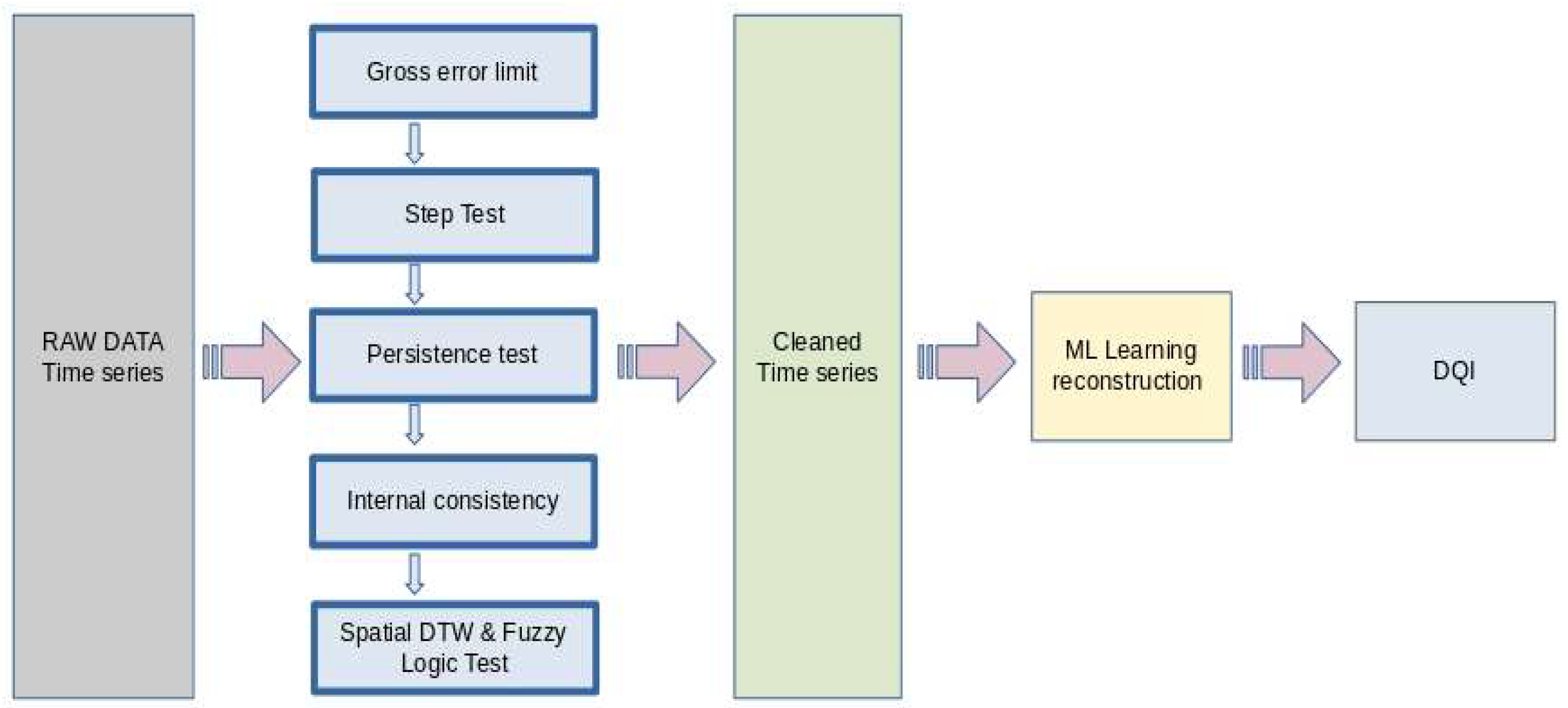
3. Materials and Methods

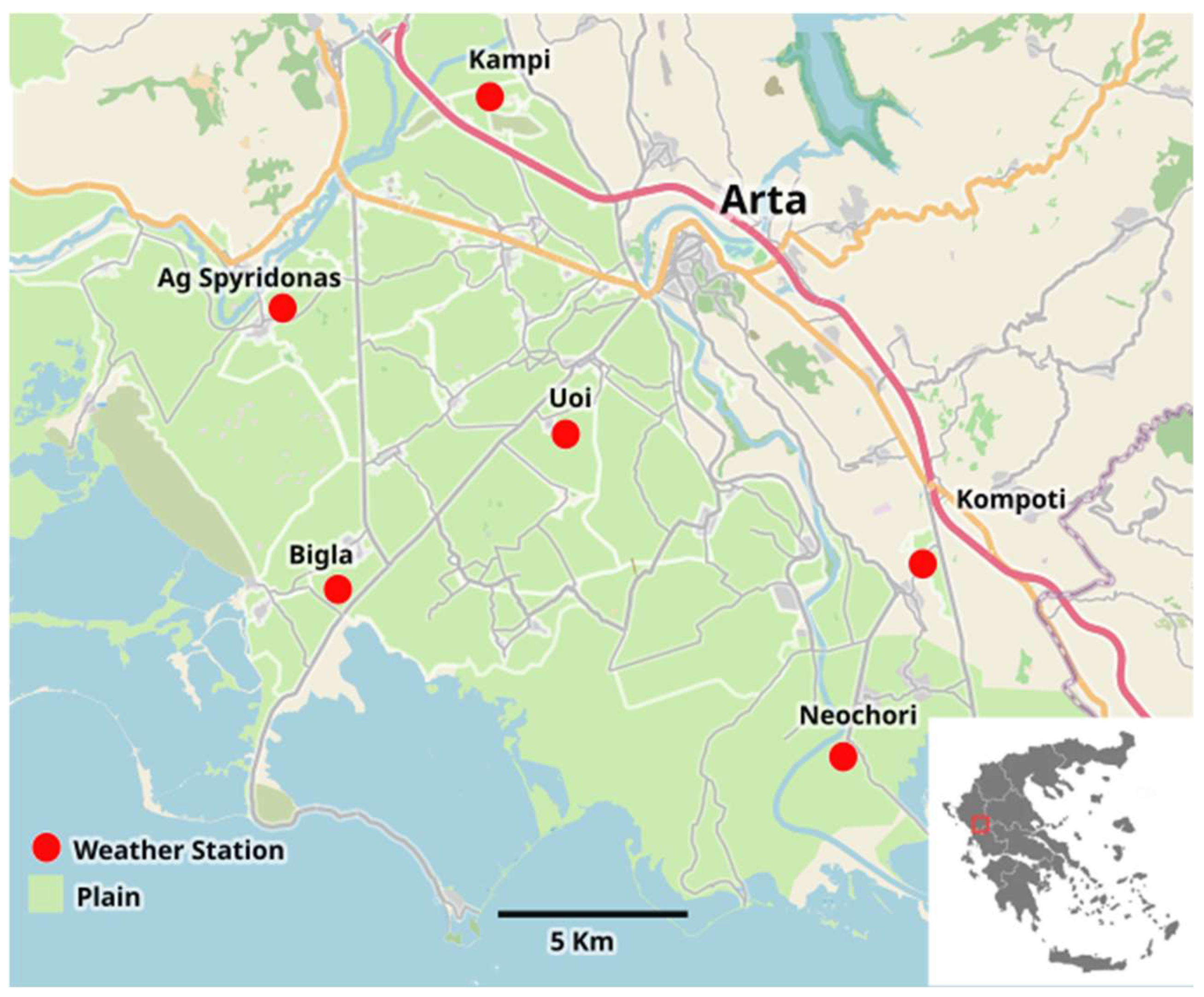
3.1. Area Description and Weather Station Network

The agrometeorological station network, located in the plain of Arta, Greece, consists of six automated weather stations that have recorded hourly temperature data for over a decade. While the network is designed to meet World Meteorological Organization’s (WMO) standards, issues such as erroneous temperature readings, extended missing data periods, and sensor degradation have been observed.

According to the WMO Guide to Meteorological Instruments and Methods of Observation [6], the representativeness of an observation is the extent to which it accurately reflects the value of a variable required for a specific application. Different uses of weather or environmental data have different requirements for how frequently data should be collected (timescales), how closely spaced weather stations should be (station density), and how detailed the observations should be (resolution). For instance, agricultural meteorology typically requires finer spatial and temporal scales than global long-range forecasting. Based on recommendations from sources such as the WMO’s Agricultural Meteorological Practices [7] and I. Orlanski [8], a representative weather station network designed for agricultural applications should ideally have a horizontal spatial scale of at least 100 m and a temporal resolution of 1 h. However, meeting these spatial requirements is challenging for weather station networks, primarily because reliable automatic weather stations that meet WMO standards are costly to purchase, install, and maintain. Furthermore, achieving a “toposcale” [6] network (100 m < Spatial density < 3 km) can be difficult. In this work, the agrometeorological station network of the Department of Agriculture of the University of Ioannina (UOI-DAGRI), which serves agricultural applications across the plain of Arta, Greece (Figure 1) (Table 1), is classified as a “mesoscale” network (3 km < spatial density < 100 km) according to WMO standards [6,7]. Weather station placement (approximately 7 km each other) places the network near the boundary between the “toposcale” (100 m–3 km) and “mesoscale” (3–100 km) domains [6,8]. While it formally falls within the mesoscale classification, its relatively dense configuration aligns more closely with the higher-resolution end of mesoscale, or even the upper range of toposcale, applications.

All of the stations of the network are identical in terms of sensor [9] type and data loggers [10]. Each station records measurements for temperature, relative humidity, solar radiation, precipitation, wind speed, and direction, as well as soil temperature and moisture. The temporal resolution requirement of 1 h [6], essential for agricultural meteorology, is met by this network. Each weather station samples data every 10 min, which can then be aggregated into 1 h intervals. Each station is positioned such that objects are not closer than twice their height above the gauge orifice, and the stations are located in areas with homogeneous dense vegetation and no ground slope.

The plain of Arta, located in Epirus, northwestern Greece, spans along the prefectures of Arta and Preveza, covering approximately 45,000 hectares. It is bordered by significant natural features: mountains to the north and east, the Gulf of Amvrakikos to the south, and the open Ionian Sea to the west. Two rivers, the Arachthos and Louros, flow through the plain. According to the Köppen–Geiger climate classification system [11], the climate of the Arta plain is categorized as “Csa”, indicating a temperate climate with dry, hot summers and mild, wet winters. This classification is consistent with the typical Mediterranean climatic patterns observed in the region. Weather patterns are influenced primarily by systems moving in from the west and northwest. Agriculture is a key activity. At low heights, annual arable crops (maize, alfalfa, etc.), citrus fruit, and kiwifruit are the main crops, while medium elevations towards the mountain ranges host olive groves, all benefiting from the varied topography and climate.

The agrometeorological stations network was installed having, as a primary goal, to support decisions regarding irrigation water management and also to feed broader agricultural consulting services and research activities. It focuses on measuring key variables for the calculation of evapotranspiration, rain, and soil moisture. Beyond irrigation water management organizations, agricultural consultants and researchers use its data for disease prevention, the calculation of chill hours, and the documentation of temperature extremes (especially frost) and other parameters that could negatively impact yield.

3.2. QC Tests

Quality control (QC) procedures for automated weather station (AWS) data are divided into three main categories: (i) pre-processing checks, (ii) basic quality control checks, and (iii) extended quality control checks. Following the guidelines provided by WMO [4,10], pre-processing checks such as syntactic validation, synchronicity, temporal repetition checks, and the handling of missing data are conducted immediately after data sampling within the AWS. These checks yield instantaneous data, typically in minute- or hourly averaged intervals, in a common text format. Basic quality control checks including gross error limits, Temporal Consistency, and Internal Consistency checks can be performed either within the AWS itself or in a digital processing center (DPC), which is the most common case. Extended quality control checks, such as Spatial Consistency, climatological constrains, homogeneity checks, or any other custom check, are exclusively carried out within the DPC as well.

In addition to the measured values of physical quantities, QC files also include metadata about the weather station. Metadata provides information on sampling methods, instrumentations, site locations, and geographical coordinates (Aguilar et al.) [12]. They also include essential instrument characteristics, such as resolution, range, measurement units, and data formats, as well as records of regular site inspections and maintenance, in accordance with the Guide to Meteorological Instruments and Methods of Observation from the WMO [6]. Validated data from these QC procedures are formatted in the NetCDF format, adhering to the international Climate and Forecast (CF) Metadata Convention version 1.7 (Eaton et al., 2003) [13], as recommended by the WMO [7].

All previously described QC tests serve as data validation steps (

Table 2. List of QC tests.

Test	Formulation	Reference
Gross error limit	−30 °C < Th < 50 °C	Shafer et al., 2000 [16]
Step Test	|Th − Th−1| < 10 °C	WMO No.8 [6]
Persistence Test	Th≠Th−1≠Th−2≠Th−3	Estévez et al. (2011) [17], Meek and Hatfield (1994) [18]
Internal Consistency	Thmin < Th < Thmax Th > Tdew (Th, RH)	WMO (2010) [7] Reek et al., 1992 [19] Feng et al. (2004) [20] Magnus-Tetens formula [21]
Spatial Consistency	T* − fσ* < Th < T* + fσ* f = 3 σ* = weighting root mean square error;	Hubbard et al. (2005) [22]
Spatial DTW and Fuzzy Logic Test		Proposed in this work
ML Reconstructed data		Proposed in this work

Th is the hourly temp value, Thmin and Thmax are the min and max hourly temp value, T* is the estimated temperature value, f is the standard deviation value, and σ* is standard deviation of the residuals.

), identifying and flagging data of questionable quality. These quality control (QC) flags supplement the data without altering them and specify which test the data failed. In certain cases, QC procedures may classify data as erroneous and remove them from further analysis, as outlined in subsequent sections. To ensure clarity and reliability, all archived meteorological data must be accompanied by QC flags (e.g., “good”, “suspect”, “warning”, or “failure”) which indicate the confidence level that network managers attribute to the observations (Fiebrich and Crawford, 2001) [14]. These flags provide users with critical information about data quality and reliability. QC flags are commonly divided into two primary categories: informative flags, which provide additional context or warnings about data quality, and severe flags, which indicate data requiring urgent attention or exclusion. This categorization is consistent with practices such as those implemented by the California Irrigation Management Information System (CIMIS) (Snyder and Pruitt, 1992) [15].

3.2.1. Basic QC: Gross Error Limit

Gross Error Limit checks are a fundamental QC test in meteorological data processing, designed to identify and eliminate physically implausible values caused by sensor malfunctions, transmission errors, or human mistakes (WMO) [6]. These checks involve defining upper and lower temperature thresholds based on historical data, instrument specifications, and regional climatic norms, such as from −30 °C to 50 °C for non-extreme climate regions [23]. Observations falling outside these limits are flagged as erroneous and are either removed or corrected, ensuring the dataset’s reliability (Durre et al., 2008) [24]. Unlike climatological limit checks, which account for seasonal and regional variations, Gross Error Limit checks rely on fixed thresholds, making them particularly suitable for short-term datasets where climatic calculations are unfeasible [6]. The data that failed this test were flagged and converted as NaN.

3.2.2. Basic QC: Step Test

The Step Test evaluates the absolute difference between consecutive temperature observations (|T_h − T_h−1|) and compares it to a predefined threshold. This method is particularly effective in identifying sudden spikes or drops that are physically implausible under normal atmospheric conditions. According to the Guide on the Global Data-Processing System (GDPS) [25], a commonly used threshold for temperature data is 4 °C or 10 °C, meaning that if the difference between two consecutive hourly measurements exceeds this value, the data point is flagged as potentially erroneous. According to a previous studies by Centrini and Estévez [3,4] for the Mediterranean region, and as also seen in our data, a temperature difference of 4 °C is too small for hourly variations and leads to a large number of failed values. For this reason, a temperature difference of 10 °C was used as a safer restriction for spike detection. The values that failed the Step Test were flagged and converted to NaN.

3.2.3. Basic QC: Persistence Test

This test evaluates whether consecutive observations exhibit identical values over a specified time period. According to Estévez et al. [3] and Meek and Hatfield [18], a common criterion for persistence tests in temperature data is to check whether four consecutive hourly measurements are identical (T_h = T_h−1 = T_h−2 = T_h−3). If this condition is met, the data points are flagged as potentially erroneous and converted to NaN. Persistence tests are particularly effective in detecting sensor freezing or data transmission failures, where the same value is recorded repeatedly over time.

3.2.4. Basic QC: Internal Consistency

Internal Consistency Tests are quality control (QC) procedures used to ensure the logical and physical coherence of meteorological data, such as temperature and humidity measurements. These tests typically involve two key components: (a) verifying that hourly temperature values (T_h) fall within the daily minimum (T_hmin) and maximum (T_hmax) temperature limits, and (b) ensuring that the hourly temperature does not exceed the dew point temperature calculated from relative humidity (RH) data. The first test, as outlined in the Guide on the Global Data-Processing System (GDPS) WMO [25], requires that T_hmin < T_h < T_hmax. However, the automatic calculation of T_hmin and T_hmax is not explicitly described in the guidelines. In this study, T_hmin and T_hmax were calculated as the mean values of the daily maximum and minimum temperatures across all operational stations. This approach relies on the assumption of spatial homogeneity within the network. This assumption can be considered reasonable because the agrometeorological stations are installed on the relatively flat and homogeneous landscape of the Arta plain at low altitudes (0–20 m) with minimal topographic influence. Moreover, Spatial Consistency Tests conducted using Dynamic Time Warping (DTW) and the Spatial Regression Test (Section 4.1) demonstrated high inter-station coherence, with pairwise RMSE values typically below 1 °C. These results confirm a strong spatial correlation among stations, supporting the use of network-averaged extreme values (T_hmin and T_hmax) for Internal Consistency checks, despite the potential presence of localized microclimatic effects.

The second test relies on the physical principle that air temperature must always be greater than or equal to the dew point temperature under normal atmospheric conditions. The dew point temperature is calculated using the Magnus–Tetens formula, as described by Lawrence [21], which provides a reliable relationship between relative humidity and dew point temperature. Any measurements that failed to pass the test were flagged and converted to NaN.

3.2.5. Basic QC: Spatial Consistency Test

All other previous QC tests were single-station tests that did not record, in advance, the neighbor temperature measurements of the other weather stations. The Spatial Consistency Test is a critical quality control procedure designed to evaluate the spatial coherence of temperature data by comparing observations from multiple stations. This test is based on the spatial regression method introduced by Hubbard et al. [22], which estimates the expected temperature at a target station using data from neighboring stations. The method calculates the residual between the observed temperature and the estimated value derived from an objective analysis, ensuring that the residual falls within a predefined confidence interval based on the selection of and standard deviation value (usually f = 3). The spatial regression test (SRT) employs a weighted average of estimates from neighboring stations, with weights determined by the strength of the relationship between the target station and its neighbors, quantified using root mean square error (RMSE) values. In addition to that, even if the spatial test provided by Hubbard is a well-defined and statistically complete method, it cannot by itself handle long periods of NaN values in addition to the possible erroneous measurements as flagged by previous tests. Another disadvantage of the method is that it calculates the estimation value of a weather station based on neighborhoods using a normal confidence distribution from the entire time series. In our case, this spatial test returned erroneous values based on certain temperature thresholds. While running the test variations, it was observed that the presence of missing data and their dependency on seasonality time windows made it very complicated for automatic use. For this reason, this test was excluded for the test sets, but the results are presented in this work. For overcoming the above problem, a new spatial test (Spatial DTW and Fuzzy Logic Test) is proposed as an alternative in this paper.

3.3. Extended QC: Spatial DTW and Fuzzy Logic Test

The challenge of comparing hourly temperature time series across multiple weather stations prompted an exploration of advanced outlier detection methods (Yaro et al.) [26] (Blázquez-García et al.) [27]. Traditional statistical approaches, such as the Z-score, Modified Z-Score, Mahalanobis Distance, One-Class SVM, and Local Outlier Factor (LOF), were initially considered. However, these methods often treat data points as independent, disregarding the strong temporal correlations inherent in temperature time series, such as daily and seasonal cycles. Furthermore, many of these techniques assume a Gaussian distribution, which may not adequately capture the characteristics of temperature data. To overcome these limitations, we introduce the “DTW and Fuzzy Logic Test”, a novel method specifically designed to detect contextual outliers in temperature data by leveraging both temporal alignment and uncertainty handling. This method combines Dynamic Time Warping algorithm and Fuzzy Logic. Unlike traditional approaches, this method utilizes the following:

• Dynamic Time Warping (DTW) to compare temperature time series across multiple stations, allowing for temporal shifts and capturing underlying similarities.
• Fuzzy Logic to handle uncertainty in anomaly classification, reducing the risk of false positives and false negatives.
• Dynamic adaptations to seasonal and diurnal temperature variations, ensuring the accurate detection of anomalies within different meteorological conditions.

3.3.1. DTW Methodology Description

The proposed anomaly detection framework integrates Dynamic Time Warping (DTW) to assess the temporal alignment and similarity between temperature time series from different weather stations [28]. DTW is a well-established technique for measuring the similarity between two time-dependent sequences by allowing for nonlinear alignments, making it particularly effective for comparing time series that exhibit shifts or distortions in time. In the context of temperature measurements, DTW enables robust comparisons across stations by accounting for variations in local meteorological conditions while preserving the overall structural integrity of the data.

A comprehensive statistical analysis of DTW distances across all station pairs revealed a right-skewed distribution (Figure 2), meaning that most temperature differences were small, but some extreme values were present. Such skewed distributions can pose challenges for defining meaningful anomaly thresholds. To address this, a logarithmic transformation (1) was applied to DTW distances to normalize the distribution, ensuring that standard statistical techniques could be effectively used for threshold determination.

log(DTW + ϵ)

(1)

where ϵ = 10⁻⁹ is a small constant introduced to prevent computational issues associated with zero-valued distances. This value was selected to be sufficiently small so as not to affect the transformation’s outcome for non-zero values. A sensitivity analysis with alternative small values (e.g., 10⁻⁸ and 10⁻¹⁰) showed no notable impact on the distribution characteristics or the resulting anomaly thresholds. Therefore, ε = 10⁻⁹ was adopted as a safe and robust default. The transformation serves two critical purposes:

• Stabilizing variance: Log transformation compresses large values and expands smaller values, reducing the influence of extreme anomalies while maintaining the relative relationships between distances.
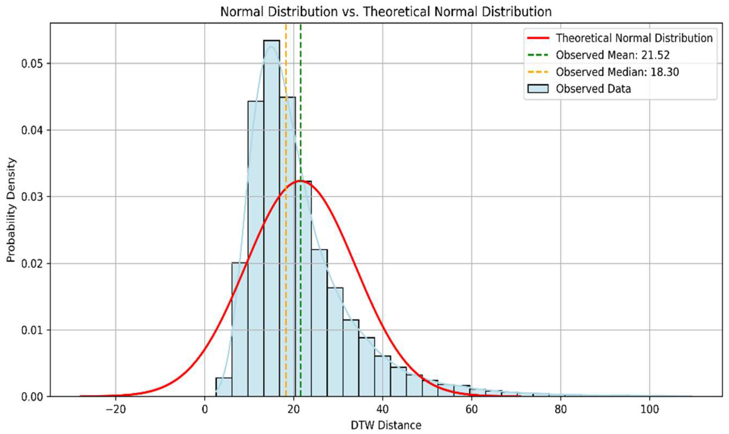
• Enhancing normality: The original DTW distance distribution exhibited a mean of 21.52 and a median of 18.30, with significant right skewness. After transformation, the distribution became more symmetric, with a mean of 2.94 and a standard deviation of 0.50, facilitating the use of standard-deviation-based thresholding techniques.

To define a statistically robust threshold for anomaly detection, the three-standard-deviation rule was applied in the log-transformed domain:

Threshold = μ + 3σ

(2)

where μ and σ represent the mean and standard deviation of the log-transformed DTW distances, respectively. This threshold was then converted back to the original scale using exponentiation:

Threshold = e^(μ+3σ) − ϵ

(3)

This resulted in a final threshold value of “85.28” in the original DTW distance scale. Any station pair exceeding this threshold was classified as an anomalous temperature relationship, indicating significant deviations in temperature patterns that warranted further investigation. The DTW framework was implemented through the following methodological steps:

• Daily isolation: Each day’s temperature data were treated as a separate time series, consisting of 24-hourly measurements per station.
• DTW pairwise comparisons: DTW distances were computed for daily temperature time series across all station pairs.
• Log transformation and thresholding: The log transformation was applied to the DTW distances, and the anomaly threshold was established using the three-standard-deviation criterion.

The application of DTW in anomaly detection is crucial, as it allows for detecting spatially and temporally inconsistent temperature variations across the network. Unlike simple Euclidean distance measures, DTW adapts to minor phase shifts in temperature variations, ensuring that stations exhibiting similar trends but with slight temporal misalignments are not falsely classified as anomalous. By integrating DTW with log transformation and statistical thresholding, the proposed framework provides a robust, scalable, and mathematically grounded method for detecting temperature anomalies, contributing to the overall Data Quality Index (DQI) for the weather station network.

3.3.2. Fuzzy Logic Model

To enhance the classification of temperature differences between weather stations, a Fuzzy Logic Model was integrated into the anomaly detection framework. This model enables a flexible and context-aware approach by considering meteorological variations and station-specific characteristics. The methodology is based on two key input variables:

• Time of day: Classified as either “Night” or “Day”.
• Absolute temperature difference: Between a reference station (e.g., Ag) and all other stations in the network.

The classification of time was determined based on hourly observations, with nighttime defined as the period between 22:00 and 08:00, while all other hours were categorized as daytime. This distinction was crucial, as diurnal temperature variations influence spatial temperature differences. To establish appropriate thresholds for anomaly detection, a statistical analysis of nighttime temperature differences between stations was conducted. Key statistical measures, including the mean, median, and percentiles, were computed. The analysis indicated that temperature differences generally remained below 10 °C at night, while deviations exceeding 11 °C were infrequent and were typically associated with sensor errors or localized meteorological effects.

Based on these findings, fuzzy membership functions were defined for each time category. For nighttime, temperature differences below 10 °C were considered normal, whereas differences exceeding 11 °C were classified as anomalies. For daytime, normal differences ranged from 0 °C to 5 °C, while values surpassing 7 °C were flagged as potential anomalies.

The Fuzzy Logic Model applied these membership functions to classify temperature observations as either normal or anomalous. A classification threshold of 1.5 was used to quantify the degree of anomaly, ensuring a robust decision-making process. This threshold represents the minimum confidence level at which a temperature difference is deemed to be an outlier, thereby mitigating the risk of false positives. Additionally, a consensus mechanism was implemented to improve reliability: an observation was flagged as anomalous only if at least three out of five station comparisons identified it as an outlier. If fewer than three stations detected an anomaly, the observation was classified as a potential false positive, requiring further verification.

The integration of Fuzzy Logic with Dynamic Time Warping (DTW) enhances anomaly detection by providing a more context-sensitive and spatially coherent assessment. DTW identifies stations with significant temporal misalignment, while Fuzzy Logic incorporates meteorological conditions to refine anomaly classification. The combined approach ensures that temperature anomalies are detected with high reliability, contributing to the overall Data Quality Index (DQI) for the weather station network. Observations failing to meet the defined criteria were systematically flagged and converted to NaN, ensuring data integrity while minimizing false detections.

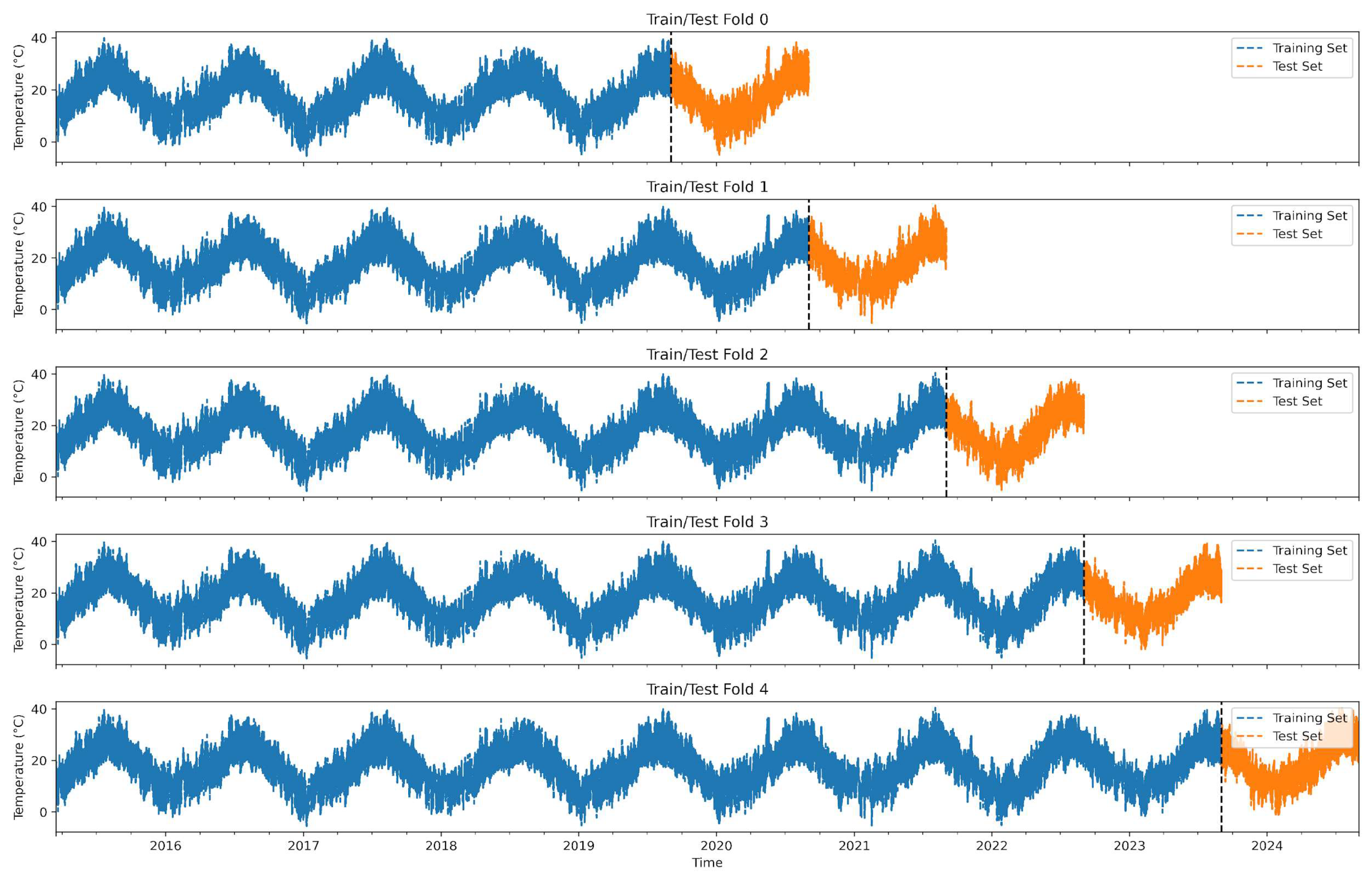
3.4. ML for the Reconstruction of Time Series

In this stage, data were validated using both basic quality control (QC) tests and the newly proposed spatial test, which integrates Dynamic Time Warping (DTW) and Fuzzy Logic, as described previously (Figure 3). Measurements that failed either the basic QC tests or the spatial test were flagged and converted to NaN, resulting in an increased number of total NaN values (

Table 3. Summary of quality control (QC) test results for each station. The table reports the absolute number of flagged cases, followed in parentheses by the percentage relative to the total dataset (N = 82,967).

Station	Initial Nan	Gross Errors	Step Test (10 °C)	Step Test (4 °C)	Persistence	Internal Consistency	Spatial Consistency	DTW Fuzzy	Final NaN
Uoi	2547 (3.07%)	0	19	2290 (2.76%)	1	0	0	4	2571 (3.1%)
Big	823	0	5	1642 (1.98%)	0	0	413 (0.5%)	0	828 (0.01%)
Ag	30	19	51	2961 (3.57%)	0	0	0	16 (0.02%)	116
Neo	8664 (10.4%)	2543 (3.07%)	51	2788 (3.35%)	0	0	0	185 (0.21%)	11,443 (13.7%)
Kom	846	20	13	4649 (5.59%)	0	0	8084 (9.73%)	21 (0.03%)	900 (0.01%)
Kam	9	0	15	2950 (3.56%)	0	0	11,370 (13.7%)	145 (0.16%)	169

Total points 82,967.

). Subsequently, a machine learning (ML) reconstruction method capable of handling NaN values was employed to impute the missing data, particularly in cases where data were missing for extended periods. This requirement is essential for two reasons:

• First, to ensure that the training dataset remains viable even if data from one station are missing.
• Second, because the final ML model—intended for real-time processing—must be able to produce results even if one or more stations are offline.

Recurrent Neural Networks (RNNs) and Tree-Based Ensemble Methods are particularly well-suited for reconstructing missing temperature values in time series datasets collected from weather stations. RNNs, especially Long Short-Term Memory (LSTM) and Gated Recurrent Units (GRU), excel at capturing temporal dependencies and learning sequential patterns, making them effective for imputing missing values based on historical temperature trends [28,29,30,31]. Additionally, their ability to adapt to real-time data streams aligns well with the requirement for continuous temperature monitoring. On the other hand, Tree-Based Ensemble Methods such as Random Forest [32], XGBoost [33], and LightGBM [34] offer strong predictive performance while inherently handling missing data, allowing for robust imputation without the need for complex preprocessing [35,36]. These models are computationally efficient, scalable, and capable of capturing nonlinear relationships in temperature variations across different stations [30].

In our study, Tree-Based Ensemble Methods, specifically XGBoost (eXtreme Gradient Boosting), were chosen for reconstructing missing values in the time series temperature dataset. XGBoost is a powerful machine learning algorithm based on gradient-boosted decision trees, designed for both classification and regression tasks. It is known for its efficiency, scalability, and ability to handle complex nonlinear relationships within the data. Unlike traditional boosting methods, XGBoost incorporates advanced optimization techniques such as second-order gradient updates, regularization (L1 and L2), and a sparsity-aware algorithm that efficiently handles missing values [5]. Various ensemble models produced comparable results based on the RMSE metric, leading the main focus to shift toward feature selection and engineering. Specifically, efforts were directed at determining the most relevant features derived from the initial dataset, such as the significance of seasonal patterns (daily, monthly, yearly) and the impact of historical values through lagged features. Identifying and incorporating these critical temporal dependencies played a key role in enhancing model performance, ensuring accurate and reliable temperature reconstructions.

For a more effective training approach and enhanced robustness against overfitting, cross-validation (Figure 4) was implemented by splitting the dataset into 80% training and 20% testing across all years. This strategy ensured that the model was evaluated on diverse temporal segments, reducing the risk of overfitting to specific periods. The final model’s performance was assessed using the median RMSE value across all cross-validation iterations, providing a more stable and reliable estimate of the reconstruction accuracy.

Among the previously mentioned models, XGBoost was found to produce nearly identical prediction results compared to the other tree-based ensemble methods. However, it demonstrated a more balanced dependency between the target station and the surrounding stations, ensuring that no single input dominated the reconstruction process. Although no formal benchmark was conducted, XGBoost was selected due to its known advantages over alternatives for the specific needs of this study. These advantages include its native handling of missing values without the need for complex data imputation, its lower computational requirements that make it suitable for CPU-only environments, its faster training and tuning times—which are especially important for near real-time reconstruction in operational networks—and its easier model interpretability, such as the ability to analyze feature importance.

All analyses in this study were conducted using Python 3.11. The implementation of machine learning reconstruction was performed using the XGBoost library, while anomaly detection incorporated Dynamic Time Warping (DTW) for time series similarity analysis. Additional data processing, quality control, and evaluation procedures were carried out using the Scikit-Learn (sklearn) library, ensuring a robust and reproducible computational framework.

3.5. DQI

Ensuring the reliability of temperature data is critical for robust meteorological analysis and climate studies. The assessment of data quality is particularly important for datasets used in decision-making, as poor-quality data can lead to erroneous conclusions and suboptimal agricultural and water management strategies. To systematically evaluate the quality of data collected from the weather station network, we introduce the Data Quality Index (DQI), a metric designed to quantify data integrity both before and after machine learning (ML) reconstruction.

The DQI incorporates two fundamental aspects of data quality, Completeness and Accuracy, providing a holistic assessment of the dataset’s usability for scientific and operational purposes. Completeness reflects the proportion of valid usable data within a given period and is a primary indicator of dataset reliability. Accuracy, on the other hand, measures the deviation of recorded values from expected values and is crucial for ensuring reliable meteorological measurements. These dimensions align with established data quality assessment frameworks. Kong et al. (2019) [37] proposed a Data Quality Evaluation Index (DQEI) to assess data quality in data journals, emphasizing Accuracy and Completeness as key dimensions of data integrity. Their work highlights the necessity for a structured approach to measuring data reliability, which is essential for environmental datasets where missing or erroneous values can significantly impact downstream analyses. Similarly, Ehrlinger et al. and Batini et al. [38,39] provided an extensive survey of data quality measurement techniques, reinforcing the importance of Completeness and Accuracy in evaluating datasets across multiple domains. Building upon these studies, our DQI framework integrates traditional quality control methods with advanced statistical and machine learning approaches to enhance both Completeness and Accuracy. By quantifying data quality improvements before and after ML-based reconstruction, the DQI provides a transparent metric for evaluating the effectiveness of data cleaning and imputation techniques.

3.5.1. Completeness Assessment

Completeness reflects the proportion of valid usable data within a given period and serves as a primary indicator of dataset reliability. Initial Missing Values, basic QC test errors, and inconsistencies identified using the DTW and Fuzzy Logic Test contribute to the data gaps that reduce completeness. Completeness can be calculated before (Initial Completeness C_init) and after (Final Completeness C_final) ML reconstruction in order for Completeness Improvement (C_imp) (5) to be calculated. We define

$$C_{init}=\left(1-{\displaystyle \frac{N_{NaN}+N_{err}+N_{DTW}}{N_{total}}}\right)\times 100$$

(4)

where

Initial Completeness, C_init, is the Completeness before ML reconstruction;

N_NaN is the count of Initial Missing Values;

N_err is the count of erroneous values;

N_DTW is the count of DTW-flagged outliers;

N_total is the total number of data points in the selected period.

Final Completeness (C_final): Since machine learning reconstruction fills all missing values and erroneous data, we assume that

$$C_{final}=100$$

Completeness Improvement (C_imp):

$$C_{imp}={\displaystyle \frac{C_{final}-C_{init}}{C_{init}}}\times 100$$

(5)

3.5.2. Accuracy Assessment

Accuracy measures the reliability of recorded temperature values by evaluating their deviation from expected values. Similarly to Completeness an initial Accuracy (A_init), final Accuracy (A_final) and Accuracy Improvement (A_imp) can be calculated. We quantify Initial Accuracy using the root mean squared error (RMSE) metric, normalized by the temperature range as follows:

$$A_{init}=100\times \left(1-{\displaystyle \frac{{RMSE}_{init}}{R_{init}}}-Penalty\right)$$

(6)

where

$R_{init}=T_{max,obs}-T_{min,obs}$ is the observed temperature range before reconstruction.

Initial RMSE (${RMSE}_{init}$) before ML reconstruction can be defined as follows:

$${RMSE}_{init}=\sqrt{{\displaystyle \frac{1}{N}}\sum {\left(T_{Final,i}-T_{obs,i}\right)}^2}$$

(7)

where

T_obs is the observed temperature before reconstruction;

T_Final is the final corrected temperature;

N is the number of valid data points.

At initial accuracy, NaN measurements cannot be included for RMSE_init calculation. In cases where, in a period of interest, only NaN errors appear, then the initial accuracy will always be 100%. To overcome this problem, we introduce a Penalty to initial accuracy according to portion of NaN values as follows:

$$Penalty=penaltyfactor\times {\displaystyle \frac{Nancount}{Totalpoints}}$$

(8)

A penalty factor of 0.1 means that, for every 1% of missing data (NaN values), the Initial Accuracy will be penalized by 0.1%. The penalty factor of 0.1 was selected as a pragmatic choice to balance penalization without excessively distorting the Initial Accuracy score. A lower factor (e.g., 0.05) would underestimate the impact of missing data, while a higher factor (e.g., 0.2) would overemphasize it. Although a formal sensitivity analysis was not conducted, preliminary tests varying the penalty factor within the range of 0.05 to 0.2 showed negligible effects on the overall DQI improvement, indicating that the selected value is robust for the intended application.

Final Accuracy (A_final): To calculate Final Accuracy, we applied the ML reconstruction RMSE results for each weather station.

$$A_{final}=100\times \left(1-{\displaystyle \frac{ML-RMSE}{R_{final}}}\right)$$

(9)

where $R_{final}=T_{max,Final}-T_{min,Final}$ is the reconstructed temperature range.

Finally, the Accuracy Improvement (A_imp) can be expressed as follows:

$$A_{imp}={\displaystyle \frac{A_{final}-A_{init}}{A_{init}}}\times 100$$

(10)

3.5.3. Data Quality Index (DQI) Computation

The overall DQI is computed as a weighted sum of completeness and accuracy as follows:

DQI = w_completeness × C+ w_accuracy × A

(11)

where equal weights (0.5) are assigned to completeness and accuracy, ensuring a balanced evaluation of data quality. We define

$$\mathrm{Initial} \mathrm{DQI}: {DQI}_{init}=\left(0.5\times C_{init}\right)+\left(0.5\times A_{init}\right)$$

(12)

$$\mathrm{Final} \mathrm{DQI}: {DQI}_{final}=\left(0.5\times C_{final}\right)+\left(0.5\times A_{final}\right)$$

(13)

The difference between DQI_final − DQI_init is expressed as percentage and can describe the overall improvement in the temperature data using ML reconstruction for a specific period of time for each station.

4. Results

4.1. Basic QC Tests’ Results

The quality control (QC) process applied to the temperature dataset from the six weather stations identified several issues, including missing values, abrupt temperature changes, and spatial inconsistencies. A summary of the results from the various QC tests is provided below (Table 3).

Initial Missing Values: The number of missing values varied significantly across the stations. Neo exhibited the highest number of missing values, totaling 8664 data points, while Kam had the fewest missing values, with only 9. These discrepancies highlight the varying quality and completeness of the data across the network.

Gross Error Check: The Gross Error Check flagged only a small fraction of the data points. Ag and Kom each had 19 and 20 flagged values, respectively. However, Neo exhibited a significantly higher number of gross errors, with 2.543 flagged cases, indicating potential sensor issues or data entry problems at this station.

Step Test: The Step Test, designed to identify abrupt temperature changes, flagged a substantial number of instances when applying a 4 °C threshold (suggested by WMO). Specifically, Kom (5.59%), Kam (3.56%), and Ag (3.57%) showed a high percentage of flagged values. Due to the inefficiency of this threshold in capturing meaningful temperature fluctuations, a stricter 10 °C threshold was applied. This adjustment resulted in significantly fewer flagged instances, with Big showing only 5 flagged cases, while both Neo and Ag had 51 flagged cases each.

Persistence Test: The persistence test, which identifies unrealistically constant temperatures, flagged only a single instance at Uoi, with all other stations passing this test. This result suggests that the temperature measurements across most stations were appropriately variable and did not exhibit prolonged periods of unrealistic stability.

Internal Consistency Test: No violations were detected in the Internal Consistency Test across any of the stations, suggesting that the data remained internally consistent within the defined temporal scope.

Spatial Consistency Check (Hubbard Test): The Spatial Consistency Check, implemented using the Hubbard spatial test, revealed significant discrepancies at two stations: Kom (9.73%) and Kam (13.7%). These stations showed higher-than-expected spatial variability, which may indicate localized deviations, sensor malfunctions, or environmental factors influencing data accuracy. However, the Hubbard test’s reliability was limited in certain cases due to the presence of missing or inconsistent data, which hindered the algorithm’s performance.

DTW–Fuzzy Spatial Test: In contrast, the newly proposed DTW–Fuzzy Spatial Test demonstrated greater adaptability to time series inconsistencies and effectively minimized false positives. This method flagged fewer problematic cases, with Neo (0.21%) and Kam (0.16%) showing the most instances of spatial inconsistency. The improved performance of this test suggests that it provides a more reliable and robust approach to Spatial Consistency checks, even in the presence of missing data.

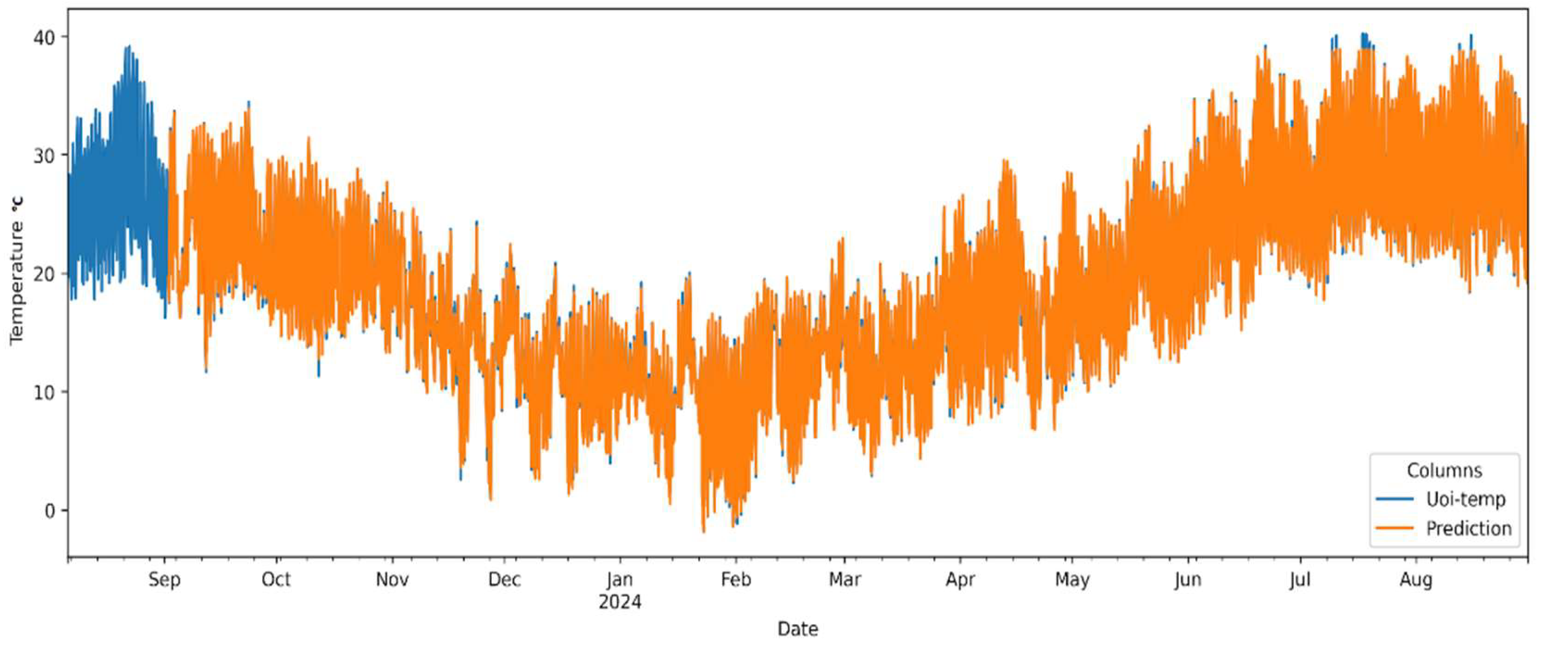
4.2. ML Reconstruction Results

Following the application of quality control (QC) procedures, machine learning (ML) techniques were employed to reconstruct missing temperature values across the weather station network. The primary objective of this reconstruction was to restore data integrity while preserving the spatial and temporal coherence of temperature observations. Among the various ML models evaluated, eXtreme Gradient Boosting (XGBoost) was selected due to its robustness in handling missing data, ability to model nonlinear relationships, and computational efficiency.

The performance of the XGBoost model was assessed using the root mean squared error (RMSE), which quantifies the deviation between the reconstructed and observed temperature values. As presented in

Table 4. ML RMSE metric value of each weather station.

	Uoi	Big	Ag	Neo	Kom	Kam
RMSE	0.43	0.40	0.42	0.47	0.66	0.52

, the RMSE values ranged from 0.40 °C to 0.66 °C, indicating high reconstruction accuracy across the network. The lowest RMSE was observed for the Big station (0.40 °C), suggesting strong agreement between the reconstructed and actual values, while the highest RMSE was recorded at Kom (0.66 °C), likely due to prolonged missing periods and localized deviations in temperature trends.

To ensure the interpretability of the reconstruction process, an analysis of feature importance was conducted. The most influential predictors for each station were identified based on their relative contribution to the model’s decision-making process. As summarized in

Table 5. Feature importance for each weather station ML model.

Station	Most Important	Less Important <10%	Min Importance <1%
Uoi	Big 49% Ag 23% Neo 13.7%	Kam 6% Kom 5% Uoi-lag1h 1.3%	Uoi-lag2h, Uoi-lag1h, Uoi-lag24h * month, quarter
Big	Uoi 48% Ag 24% Neo 17%	Kam 6% Big-lag1h 2%	Kom, Big-lag2h, Big-lag1h, Big-lag24h month quarter
Ag	Big 37% Kam 35% Uoi 19.5%	Neo 3% Ag-lag1h 2.6%	Kom, Ag-lag2h, Ag-lag1h, Ag-lag24h month, quarter
Neo	Kom 38% Uoi 32% Big 23%	Ag 2.6% Neo-lag1h 2.5%	Kam Neo-lag1h, Neo-lag2h, Neo-lag24h month, quarter
Kom	Neo 59% Uoi 25%	Ag 6.5% Kom-lag1h 4% Big 3.6%	Kam Kom-lag1h, Kom-lag2h, Kom-lag24h month, quarter
Kam	Ag 46% Uoi 25% Big 14% Kam-lag1h 10%	Kom 1.5% Neo 1%	Kam lag2h, Kam-lag1h, Kam-lag24h month, quarter

* lag_1h, lag_2h, and lag_24h represent the 1 h, 2 h, and 24 h previous temperature values.

, the reconstructed values at each station were primarily influenced by neighboring stations, reinforcing the assumption of spatial coherence in temperature variations. These results demonstrate that spatial correlation played a crucial role in the reconstruction process, as temperature values at a given station were strongly dependent on observations from nearby locations. Furthermore, temporal dependencies, such as lagged temperature values from previous hours, contributed to the reconstruction, but had a relatively lower impact (<10%) compared to spatial features. The ML-based reconstruction approach effectively restored missing temperature values (Figure 5) while maintaining spatial and Temporal Consistency. The key findings of this analysis can be summarized as follows:

• The XGBoost model achieved high reconstruction accuracy, with RMSE values ranging between 0.40 °C and 0.66 °C across the weather station network.
• The Big station exhibited the lowest RMSE (0.40 °C), indicating stable temperature patterns and a strong spatial correlation with neighboring stations.
• The Kom station recorded the highest RMSE (0.66 °C), suggesting that prolonged missing data periods and localized temperature anomalies may have introduced higher reconstruction uncertainty.
• Spatial correlation was the dominant factor influencing reconstruction accuracy, with temperature observations from nearby stations serving as the most significant predictors.
• The proposed method provides a computationally efficient and interpretable solution for reconstructing missing meteorological data, offering a practical framework for ensuring data completeness in automated weather station networks.

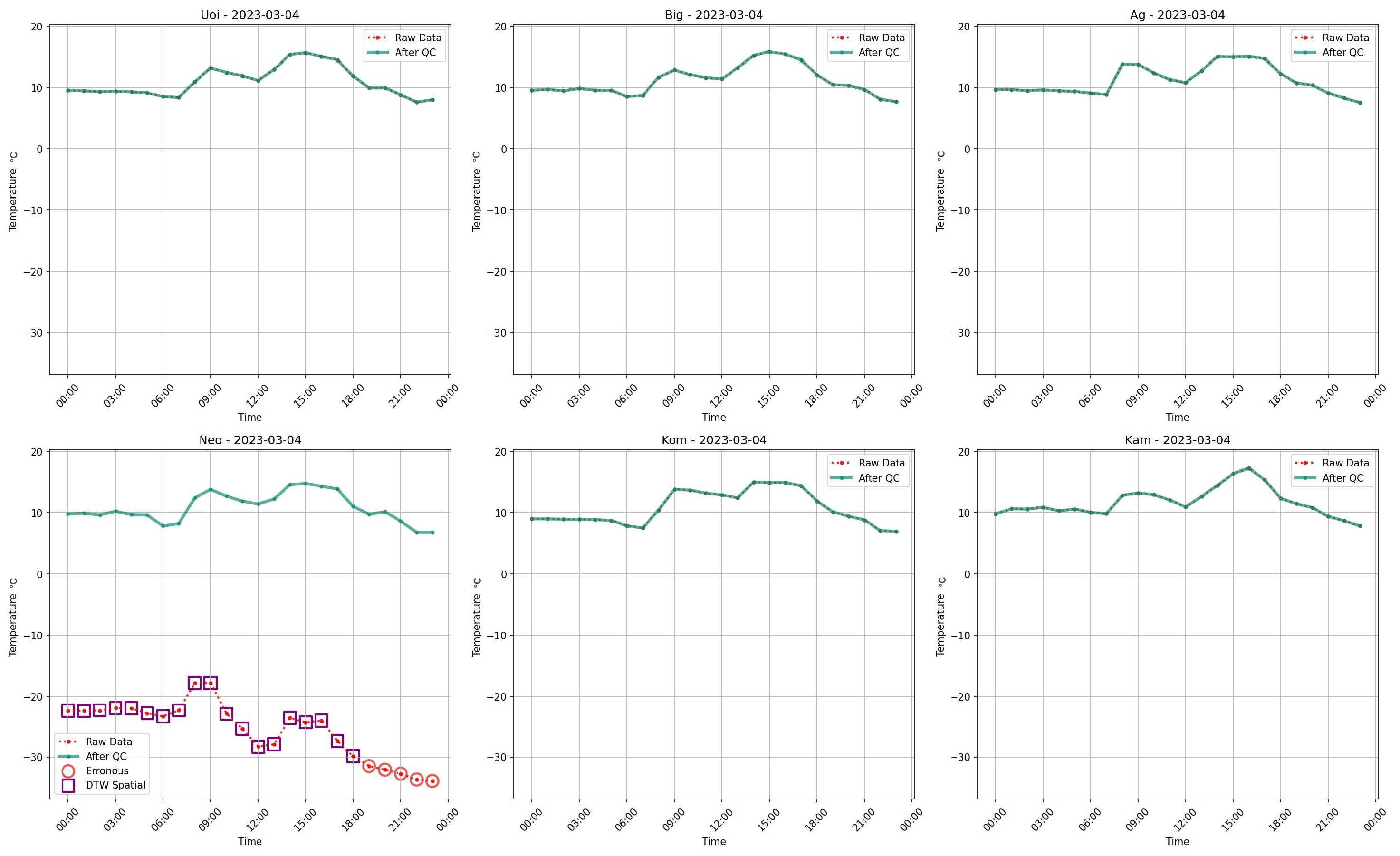
4.3. Results of the Proposed DTW–Fuzzy Spatial Test

The DTW–Fuzzy Spatial Test was applied to the quality-controlled temperature dataset to identify spatial inconsistencies across the weather station network. This method demonstrated superior robustness compared to the traditional Hubbard Spatial Consistency Test, particularly in handling missing data and seasonal variations.

Table 6. DTW–Fuzzy Spatial Test total number of anomalies for each station.

Station	Anomalies Detected (n)	Anomalies Detected (%)
Uoi	4	0.005%
Big	0	0.000%
Ag	16	0.02%
Neo	185	0.21%
Kom	21	0.03%
Kam	145	0.16%

summarizes the number and percentage of anomalies detected using the DTW–Fuzzy Spatial Test for each station.

The DTW–Fuzzy test detected a very small percentage of spatial anomalies, suggesting strong coherence across the network, but was still able to identify critical localized deviations that traditional methods overlooked. An example of the DTW–Fuzzy Spatial Test’s enhanced sensitivity is shown in Figure 6, which displays the all-station temperature time series on 4 March 2023.

On this day, the Neo station exhibited abnormal behavior not captured with the traditional Hubbard spatial test and partially captured from base QC tests, but clearly detected using the DTW–Fuzzy framework.

Unlike the Hubbard method, which relies on static thresholds and can be biased by missing data, the DTW–Fuzzy approach dynamically adapts to the observed temporal structures, minimizing false positives while improving the reliability of anomaly detection. Overall, the DTW–Fuzzy method demonstrated the following:

• Better resilience to missing values.
• Higher detection sensitivity to local anomalies.
• Lower false alarm rates, improving the trustworthiness of spatial quality control assessments.

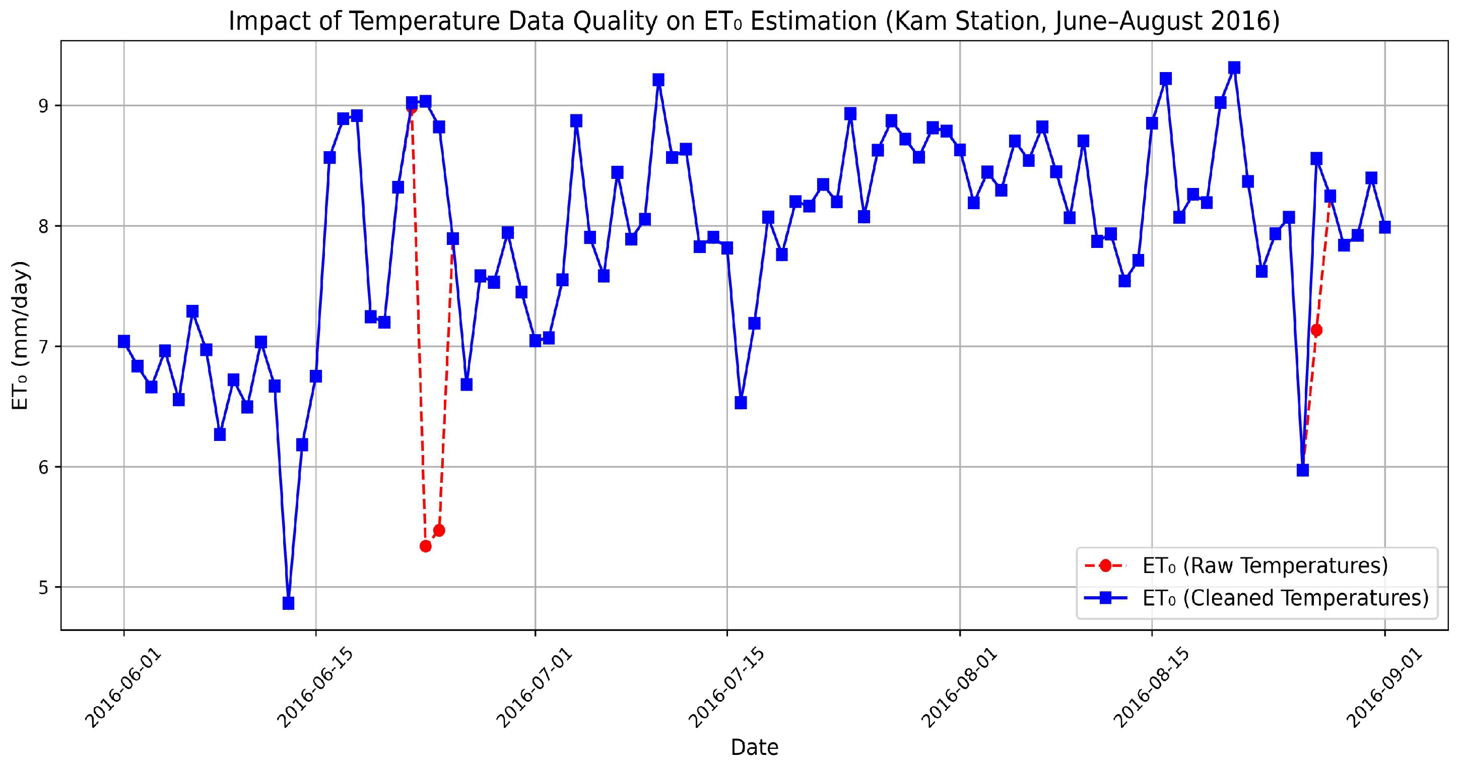
4.4. Preliminary Assessment of Temperature Data Quality Impact on Evapotranspiration Estimation

To illustrate the practical significance of improved temperature data quality for agricultural decision-making, a preliminary assessment of the impact on evapotranspiration (ET) estimation was conducted. The Hargreaves–Samani method [40], which calculates reference evapotranspiration (ET₀) based primarily on air temperature data and extraterrestrial radiation, was selected due to its widespread use and sensitivity to temperature accuracy [41,42].

ET₀ = 0.0023 (T_mean + 17.8) (T_max − T_min)^0.5 R_a

(14)

where ET₀ is the reference evapotranspiration (mm/day) and T_mean, T_max, and T_min are the mean, maximum, and minimum daily temperatures (°C), respectively. The constant 0.0023 and coefficient 17.8 were empirically derived using the Hargreaves–Samani method. Finally, Ra stands for extraterrestrial radiation (MJ/m²/day).

Using data from “Kam” weather station, characterized by erroneous temperature records, ET₀ was computed using both the raw and cleaned temperature datasets. The results reveal substantial differences in ET₀ estimation between the raw and cleaned datasets, particularly during periods associated with sensor errors. For example, on 23 June 2016, the cleaned temperature series produced an ET₀ value of 9.0 mm/day, compared to 5.31 mm/day calculated from the raw data (Figure 7). These discrepancies were mainly attributed to extreme erroneous temperature values and periods of missing data, which the reconstruction framework effectively corrected.

This preliminary analysis confirms that the enhanced temperature data not only improve Internal Consistency, but also have a direct and measurable positive effect on evapotranspiration modeling outcomes. Future work will systematically assess ET₀ estimation improvements across the entire dataset and integrate the enhanced data into irrigation scheduling decision support systems.

4.5. DQI Results

The Data Quality Index (DQI) was developed to offer a quantitative measure of the reliability of temperature data, empowering end users such as farmers, irrigation specialists, and researchers to make informed decisions. By integrating completeness and accuracy metrics, the DQI provides a comprehensive evaluation of data quality, ensuring transparency and usability for agricultural and water management applications. The initial DQI (DQI_init), computed before data reconstruction, reflects the quality of the raw data, highlighting missing values, sensor malfunctions, and flagged anomalies. The final DQI (DQI_final), calculated after machine learning (ML) reconstruction, indicates the extent to which data quality has been restored, serving as a metric for the effectiveness of the applied reconstruction techniques.

Figure 8 illustrates the total number of problematic temperature measurements over time, including missing values (NaN), erroneous readings, and those flagged by the DTW–Fuzzy method. This plot allows us to identify the Longest Problematic Period (LPP) for each weather station, which highlights extended periods of data gaps and errors. By incorporating the LPP into the Data Quality Index (DQI) calculation, we can assess how data quality improves when these periods are addressed. This approach provides the highest data improvement, making it an effective method for evaluating and enhancing overall data quality.

Table 7. “Longest Problematic Period” of each station.

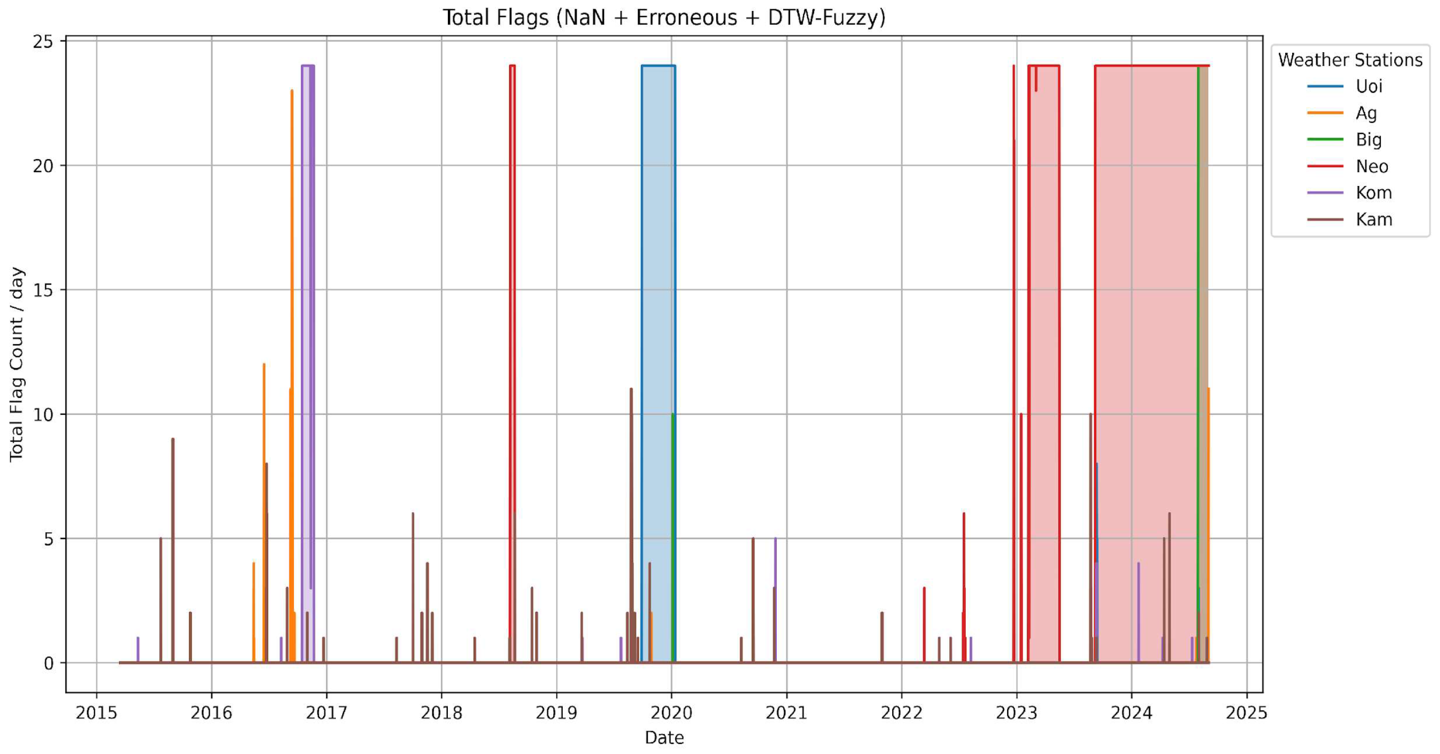
	Start	End	Nan	Erroneous	DTW-Fuzzy
Uoi	27 July 2019	11 January 2020	2	2542	1
Ag	14 June 2016	12 September 2016	55	13	7
Big	29 July 2024	31 August 2024	0	809	0
Neo	2 March 2023	31 August 2024	1663	8659	120
Kom	13 October 2016	20 November 2016	22	842	4
Kam	23 August 2019	24 August 2019	0	0	13

summarizes the longest problematic periods at each weather station. The durations of these periods, along with their corresponding error counts, are provided for each station, giving insight into the severity of data quality issues.

Following the analysis of problematic periods, the completeness of the dataset was evaluated by examining the proportion of missing values, erroneous measurements, and flagged anomalies in the entire recorded temperature time series. The initial completeness (C_init) reflects the proportion of usable data prior to reconstruction, while the final completeness (C_final) assumes a fully restored dataset after ML-based imputation. Similarly, the accuracy of the dataset was assessed using the root mean squared error (RMSE) normalized with the observed temperature range. The initial accuracy (A_init) was computed based on the pre-reconstruction data, while the final accuracy (A_final) was based on the station-specific RMSE of the ML-reconstruction model. The results are presented in

Table 8. DQI improvement in the “Longest Problematic Period” of each station.

	Initial Completeness	Final Completeness	Initial Accuracy	Final Accuracy	Initial DQI	Final DQI	Improvement
Uoi	37.25%	100.00%	68.66%	98.79%	52.96%	99.40%	46.44%
Ag	96.57%	100.00%	99.70%	98.46%	98.13%	99.23%	1.10%
Big	0.61%	100.00%	50.31%	83.59%	25.46%	91.79%	66.33%
Neo	20.72%	100.00%	67.14%	98.86%	43.93%	99.43%	55.50%
Kom	7.26%	100.00%	55.02%	97.74%	31.14%	98.87%	67.73%
Kam	72.92%	100.00%	100.00%	100.00%	86.46%	99.98%	13.52%

. Furthermore, an overall improvement in DQI is presented in

Table 9. Overall DQI improvement of each station (2015–2024).

	Initial Completeness	Final Completeness	Initial Accuracy	Final Accuracy	Initial DQI	Final DQI	Improvement
Uoi	99.90%	100.00%	98.47%	99.06%	97.68%	99.53%	1.85%
Ag	99.86%	100.00%	99.98%	99.09%	99.93%	99.54%	−0.39%
Big	99.00%	100.00%	99.50%	99.07%	99.25%	99.53%	0.28%
Neo	86.21%	100.00%	94.78%	99.10%	90.49%	99.55%	9.06%
Kom	98.92%	100.00%	99.49%	99.15%	99.20%	99.57%	0.37%
Kam	99.80%	100.00%	99.99%	99.15%	99.90%	99.58%	−0.32%

, using the entire time period from 2015 to 2024.

“Final Completeness” refers solely to the absence of missing (empty) data after machine learning (ML) reconstruction. “Final Accuracy” represents the accuracy of the reconstructed temperature values, assessed using the RMSE metric normalized with the temperature range.

For stations with initially high data quality, such as Ag and Kam, a slight decrease in the overall Data Quality Index (DQI) was observed following machine learning (ML) reconstruction. This effect is explained by the fact that ML models, despite their high predictive accuracy (RMSE 0.40–0.66 °C), inevitably introduce small deviations relative to the original measurements. When applied to already high-quality data, these minor inaccuracies slightly reduce the accuracy component of the DQI. Given that the DQI formula equally weights completeness and accuracy, this marginal loss offsets the completeness gain. This observation suggests that, for datasets with near-perfect initial conditions, a more targeted reconstruction strategy may be preferable, but this will be explored in a future work.

5. Discussion

This study presents a data quality assessment framework for hourly temperature data collected from a six-station agrometeorological network operating on the plain of Arta (Epirus, Greece). This study covers the period from 2015 to 2023. The application of Dynamic Time Warping (DTW) and Fuzzy Logic notably improved the spatial anomaly detection process. Compared to conventional Spatial Consistency checks such as the Hubbard Test, which exhibited sensitivity to missing values and rigid assumptions about distribution, the DTW–Fuzzy framework provided a more flexible and context-aware solution. Its robustness against missing data and capacity to dynamically adapt to diurnal and seasonal temperature patterns significantly reduced false positives, a critical advantage for automated data quality pipelines. The machine-learning-based reconstruction using XGBoost also demonstrated high performance, with RMSE values ranging from 0.40 °C to 0.66 °C.

A practical consideration, which is outlined by the results, is that at least two—or, preferably, three—weather stations must be operational in an area in order to safeguard data quality, a suggestion that aligns with other relevant studies [43]. This recommendation is directly supported by the operational principles of the DTW–Fuzzy Logic anomaly detection framework proposed in this study. Since the DTW algorithm assesses the similarity between temperature time series from different stations, and the Fuzzy Logic Model refines anomaly detection based on multiple cross-comparisons, having multiple stations operational simultaneously significantly strengthens the robustness and reliability of outlier identification. When only a single neighboring station is available, the capacity to distinguish between true anomalies and localized meteorological variations is reduced. Therefore, the simultaneous operation of at least two, and ideally three, weather stations within weather station network is critical to maintain high spatial redundancy, enhance anomaly detection sensitivity, and safeguard overall data quality.

The introduction and implementation of the Data Quality Index (DQI) represent a critical advancement in quantifying data reliability. By considering both Completeness and Accuracy, the DQI offers a holistic and interpretable metric. Significant improvements in the DQI were observed across stations with problematic periods where the initial DQI scores were substantially lower due to extensive missing and erroneous data. After ML reconstruction, these stations showed marked improvements (up to 67.7%), validating the efficacy of the proposed framework. For stations with already high data quality, the minor reduction in the DQI highlights a key consideration: ML-based reconstruction, while beneficial for filling gaps, may introduce slight deviations in otherwise high-fidelity data. This finding suggests that future implementations should include conditional reconstruction strategies, perhaps based on station-level DQI thresholds or uncertainty estimations.

The proposed approach has very significant applications regarding agricultural decision-making. As the number of personal weather stations for agricultural purposes is booming, the proposed approach could find an extensive field of application that regards data quality assessment and provision of improved data time series. An indicative field of application is irrigation water management, as evapotranspiration (ET₀) calculation has been proven to be sensitive to temperature data quality in studies all around the world for methods that use a set of measured parameters [44] as well as for methods that are based only on temperature measurements [45]. A preliminary analysis of the impact of data quality on evapotranspiration estimation using the Hargreaves–Samani method demonstrated substantial differences in outputs between raw and cleaned datasets. This highlights the real-world implications of poor-quality temperature data on critical agricultural processes such as irrigation planning. The cleaned data yielded more consistent and credible ET₀ values, affirming that improvements in temperature data quality translate directly into enhanced decision support.

Planning for future research includes the application of the proposed approach for other parameters such as relative humidity and rain and its combination with remote sensing data for the creation of virtual agro-meteorological stations. Initially, the extension of the framework to other variables (e.g., humidity) will be carried out independently; nonetheless, future work will also investigate multivariate modeling strategies to assess the potential benefits for anomaly detection and reconstruction. Scalability challenges, such as the computational cost of multi-variable modeling, are expected to be manageable, as both the Dynamic Time Warping (DTW) method and the XGBoost model demonstrated fast computational performance during this study.

6. Conclusions

This study presents a robust framework for improving the quality of hourly temperature data collected from a six-station agrometeorological network in Epirus, Greece. By integrating traditional quality control (QC) methods with advanced techniques such as Dynamic Time Warping (DTW), Fuzzy Logic, and XGBoost machine learning, we address key challenges related to missing values, sensor errors, and spatial inconsistencies. The proposed DTW–Fuzzy Logic anomaly detection method effectively identifies contextual outliers, while ML-based reconstruction significantly improves data completeness and accuracy, achieving RMSE values as low as 0.40 °C.

The introduction of a Data Quality Index (DQI) allowed for a quantitative assessment of data reliability, demonstrating substantial improvements after reconstruction. These advancements directly benefit agricultural decision-making, particularly in irrigation water management and crop modeling, where precise temperature data are essential for evapotranspiration (ETo) calculations and yield predictions. The integration of high-quality temperature data into decision-support systems (DSS) enables farmers, irrigation specialists, and researchers to make more informed and resource-efficient choices, ultimately contributing to sustainable agriculture. While this framework significantly enhances data quality, further improvements could be explored:

• Extending the DQI framework to incorporate additional meteorological variables such as humidity, solar radiation, and wind speed.
• Exploring alternative machine learning models (e.g., LSTMs, transformers) for even more robust time series reconstructions.
• Evaluating the impact of improved data quality on real-world irrigation practices using field experiments and case studies.

By continuously refining temperature data quality assessment methods, we can further support climate-resilient and data-driven agricultural practices, ensuring optimal water use.

References

- Faybishenko, B.; Versteeg, R.; Pastorello, G.; Dwivedi, D.; Varadharajan, C.; Agarwal, D. Challenging problems of quality assurance and quality control (QA/QC) of meteorological time series data. Stoch. Environ. Res. Risk Assess. 2022, 36, 1049–1062. [Google Scholar] [CrossRef]
- Lopez-Guerrero, A.; Cabello-Leblic, A.; Fereres, E.; Vallee, D.; Steduto, P.; Jomaa, I.; Owaneh, O.; Alaya, I.; Bsharat, M.; Ibrahim, A.; et al. Developing a Regional Network for the Assessment of Evapotranspiration. Agronomy 2023, 13, 11. [Google Scholar] [CrossRef]
- Estévez, J.; Gavilán, P.; Berengena, J. Sensitivity analysis of a Penman–Monteith type equation to estimate reference evapotranspiration in southern Spain. Hydrol. Process. 2009, 23, 3342–3353. [Google Scholar] [CrossRef]
- Cerlini, P.; Silvestri, L.; Saraceni, M. Quality control and gap-filling methods applied to hourly temperature observations over Central Italy. Meteorol. Appl. 2020, 27, e1913. [Google Scholar] [CrossRef]
- Boujoudar, M.; El Ydrissi, M.; Abraim, M.; Bouarfa, I.; El Alani, O.; Ghennioui, H.; Bennouna, E.G. Comparing machine learning algorithms for imputation of missing time series in meteorological data. Neural Comput. Appl. 2024. [Google Scholar] [CrossRef]
- WMO. Guide to Meteorological Instruments and Methods of Observation; No. 8; WMO: Geneva, Switzerland, 2023. [Google Scholar]
- WMO. Guide to Agricultural Meteorological Practices (GAMP); No. 134; WMO: Geneva, Switzerland, 2010. [Google Scholar]
- Orlanski, I. A rational subdivision of scales for atmospheric processes. Bull. Am. Meteorol. Soc. 1975, 56, 527–530. [Google Scholar]
- High Precision Miniature Humidity and Temperature Probe. Available online: https://www.epluse.com/products/humidity-instruments/humidity-modules-and-probes/ee08 (accessed on 29 March 2025).
- A753 UHF Radio Telemetry Unit. ADCON. Available online: https://www.rshydro.fr/wireless-telemetry-systems/wireless-radio-data-loggers/radio-rtus/a753-uhf-radio-telemetry-unit/ (accessed on 29 March 2025).
- Peel, M.C.; Finlayson, B.L.; McMahon, T.A. Updated world map of the Köppen-Geiger climate classification. Hydrol. Earth Syst. Sci. 2007, 11, 1633–1644. [Google Scholar] [CrossRef]
- Aguilar, E.; Auer, I.; Brunet, M.; Peterson, T.; Wieringa, J. Guidelines on Climate Metadata and Homogenization; No. 1186; WMO: Geneva, Switzerland, 2003. [Google Scholar]
- Eaton, B.; Gregory, J.; Drach, B.; Taylor, K.; Hankin, S.; Caron, J.; Signell, R.; Bentley, P.; Rappa, G.; Höck, H.; et al. NetCDF Climate and Forecast (CF) Metadata Conventions. NetCDF. Available online: https://cfconventions.org/cf-conventions/cf-conventions.html (accessed on 29 March 2025).
- Fiebrich, C.; Crawford, K. The Impact of Unique Meteorological Phenomena Detected by the Oklahoma Mesonet and ARS Micronet on Automated Quality Control. Bull. Am. Meteorol. Soc. 2001, 82, 2173–2188. [Google Scholar] [CrossRef]
- Snyder, R.L.; Pruitt, W.O. Evapotranspiration data management in California. In Proceedings of the Irrigation and Drainage Sessions at Water Forum ‘92, Baltimore, ML, USA, 2–6 August 1992; pp. 128–133. [Google Scholar]
- Shafer, M.A.; Fiebrich, C.A.; Arndt, D.S.; Fredrickson, S.E.; Hughes, T.W. Quality assurance procedures in the Oklahoma Mesonet. J. Atmos. Ocean. Technol. 2000, 17, 474–494. [Google Scholar] [CrossRef]
- Estévez, J.; Gavilán, P.; Giráldez, J.V. Guidelines on validation procedures for meteorological data from automatic weather stations. J. Hydrol. 2011, 402, 144–154. [Google Scholar] [CrossRef]
- Meek, D.; Hatfield, J. Data Quality Checking for Single Station Meteorological Databases. Agric. For. Meteorol. 1994, 69, 85. [Google Scholar] [CrossRef]
- Reek, T.; Doty, S.R.; Owen, T.W. A deterministic approach to the validation of historical daily temperature and precipitation data from the Cooperative Network. Bull. Am. Meteorol. Soc. 1992, 73, 753–762. [Google Scholar] [CrossRef]
- Feng, S.; Hu, Q.; Qian, Q. Quality control of daily meteorological data in China, 1951–2000: A new dataset. Int. J. Climatol. 2004, 24, 853–870. [Google Scholar] [CrossRef]
- Lawrence, M. The Relationship between Relative Humidity and the Dewpoint Temperature in Moist Air: A Simple Conversion and Applications. Bull. Am. Meteorol. Soc. 2005, 86, 225–233. [Google Scholar] [CrossRef]
- Hubbard, K.G.; You, J. Spatial regression test for climate data. J. Appl. Meteorol. 2005, 44, 634–643. [Google Scholar]
- Fiebrich, C.A.; Morgan, C.R.; McCombs, A.G.; Hall, P.K.; McPherson, R.A. Quality assurance procedures for mesoscale meteorological data. J. Atmos. Ocean. Technol. 2010, 27, 1565–1582. [Google Scholar] [CrossRef]
- Durre, I.; Menne, M.J.; Vose, R.S. Strategies for evaluating quality assurance procedures. J. Appl. Meteorol. Climatol. 2008, 47, 1785–1791. [Google Scholar] [CrossRef]
- WMO. Guide on the Global Data-Processing System; No. 305; WMO: Geneva, Switzerland, 1993. [Google Scholar]
- Yaro, A.S.; Maly, F.; Prazak, P. Outlier Detection in Time-Series Receive Signal Strength Observation Using Z-Score Method with Sn Scale Estimator for Indoor Localization. Appl. Sci. 2023, 13, 6. [Google Scholar] [CrossRef]
- Blázquez-García, A.; Conde, A.; Mori, U.; Lozano, J. A Review on Outlier/Anomaly Detection in Time Series Data. ACM Comput. Surv. 2021, 54, 56. [Google Scholar] [CrossRef]
- Li, K.; Sward, K.; Deng, H.; Morrison, J.; Habre, R.; Franklin, M.; Chiang, Y.-Y.; Ambite, J.L.; Wilson, J.P.; Eckel, S.P. Using dynamic time warping self-organizing maps to characterize diurnal patterns in environmental exposures. Sci. Rep. 2021, 11, 24052. [Google Scholar] [CrossRef]
- Hochreiter, S.; Schmidhuber, J. Long Short-Term Memory. Neural Comput. 1997, 9, 1735–1780. [Google Scholar] [CrossRef] [PubMed]
- Li, C.; Ren, X.; Zhao, G. Machine-Learning-Based Imputation Method for Filling Missing Values in Ground Meteorological Observation Data. Algorithms 2023, 16, 9. [Google Scholar] [CrossRef]
- Hayawi, K.; Shahriar, S.; Hacid, H. Climate Data Imputation and Quality Improvement Using Satellite Data. J. Data Sci. Intell. Syst. 2025, 3, 2. [Google Scholar] [CrossRef]
- RandomForestClassifier. Scikit-Learn. Available online: https://scikit-learn.org/stable/modules/generated/sklearn.ensemble.RandomForestClassifier.html (accessed on 29 March 2025).
- XGBoost Documentation—Xgboost 3.0.0 Documentation. Available online: https://xgboost.readthedocs.io/en/release_3.0.0/ (accessed on 29 March 2025).
- LightGBM Documentation. Available online: https://lightgbm.readthedocs.io/en/stable/ (accessed on 29 March 2025).
- Friedman, J.H. Greedy function approximation: A gradient boosting machine. Ann. Stat. 2001, 29, 1189–1232. [Google Scholar] [CrossRef]
- Chen, T.; Guestrin, C. XGBoost: A Scalable Tree Boosting System. In Proceedings of the 22nd ACM SIGKDD International Conference on Knowledge Discovery and Data Mining, KDD ’16, San Francisco, CA, USA, 13–17 August 2016; Association for Computing Machinery: New York, NY, USA, 2016; pp. 785–794. [Google Scholar] [CrossRef]
- Kong, L.; Xi, Y.; Lang, Y.; Wang, Y.; Zhang, Q. A Data Quality Evaluation Index for Data Journals. In Big Scientific Data Management; BigSDM 2018. Lecture Notes in Computer Science; Springer: Cham, Switzerland, 2019; Volume 11473. [Google Scholar] [CrossRef]
- Ehrlinger, L.; Wöß, W. A Survey of Data Quality Measurement and Monitoring Tools. Front. Big Data 2022, 5, 850611. [Google Scholar] [CrossRef]
- Batini, C.; Barone, D.; Mastrella, M.; Maurino, A.; Ruffini, C. A Framework and a Methodology for Data Quality Assessment and Monitoring. In Proceedings of the 12th International Conference on Information Quality, MIT, Cambridge, MA, USA, 9–11 November 2007; p. 346. [Google Scholar]
- Hargreaves, G.H.; Samani, Z.A. Reference crop evapotranspiration from temperature. Appl. Eng. Agric. 1985, 1, 96–99. [Google Scholar] [CrossRef]
- Liu, H.; Zhang, R.; Li, Y. Sensitivity analysis of reference evapotranspiration (ETo) to climate change in Beijing, China. Desalin. Water Treat. 2014, 52, 2799–2804. [Google Scholar] [CrossRef]
- Emeka, N.; Ikenna, O.; Okechukwu, M.; Chinenye, A.; Emmanuel, E. Sensitivity of FAO Penman–Monteith Reference Evapotranspiration (ETo) to Climatic Variables Under Different Climate Types in Nigeria. J. Water Clim. Change 2021, 12, 858–878. [Google Scholar] [CrossRef]
- Stahl, K.; Moore, R.D.; Floyer, J.A.; Asplin, M.G.; McKendry, I.G. Comparison of approaches for spatial interpolation of daily air temperature in a large region with complex topography and highly variable station density. Agric. For. Meteorol. 2006, 139, 224–236. [Google Scholar] [CrossRef]
- Paredes, P.; Pereira, L.S.; Almorox, J.; Darouich, H. Reference grass evapotranspiration with reduced data sets: Parameterization of the FAO Penman-Monteith temperature approach and the Hargeaves-Samani equation using local climatic variables. Agric. Water Manag. 2020, 240, 106210. [Google Scholar] [CrossRef]
- Tegos, A.; Malamos, N.; Efstratiadis, A.; Tsoukalas, I.; Karanasios, A.; Koutsoyiannis, D. Parametric Modelling of Potential Evapotranspiration: A Global Survey. Water 2017, 9, 795. [Google Scholar] [CrossRef]