Author Contributions
Methodology, H.L.; writing—original draft preparation, H.L.; experiment, J.N.; software, J.N.; review and editing, J.L. (Jaecheon Lee); conceptualization, S.L.; investigation, H.Z.; resources, J.L. (Jiantao Lu); validation, C.C. All authors have read and agreed to the published version of the manuscript.
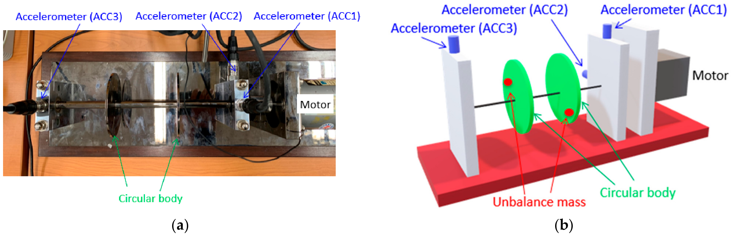
Figure 1.
Experimental rotor testbench. (a) Photograph of the actual testbench. The motor is located at the right end; ACC1 is vertically mounted at the right bearing support, ACC2 horizontally at the same support, and ACC3 vertically at the left bearing support. (b) Schematic overview showing shaft, two unbalance discs, bearing supports, and accelerometer positions of ACC1 to ACC3.
Figure 1.
Experimental rotor testbench. (a) Photograph of the actual testbench. The motor is located at the right end; ACC1 is vertically mounted at the right bearing support, ACC2 horizontally at the same support, and ACC3 vertically at the left bearing support. (b) Schematic overview showing shaft, two unbalance discs, bearing supports, and accelerometer positions of ACC1 to ACC3.
Figure 2.
Schematic diagrams of the four rotor configurations (red, green, and blue colors mean unbalance masses, disks, and a rotary shaft, respectively). (a) Balance (B): no added mass. (b) Static left unbalance (SL): unbalance mass on the left disc only. (c) Static right unbalance (SR): unbalance mass on the right disc only. (d) Dynamic unbalance (D): equal masses on both discs with 180° phase offset.
Figure 2.
Schematic diagrams of the four rotor configurations (red, green, and blue colors mean unbalance masses, disks, and a rotary shaft, respectively). (a) Balance (B): no added mass. (b) Static left unbalance (SL): unbalance mass on the left disc only. (c) Static right unbalance (SR): unbalance mass on the right disc only. (d) Dynamic unbalance (D): equal masses on both discs with 180° phase offset.
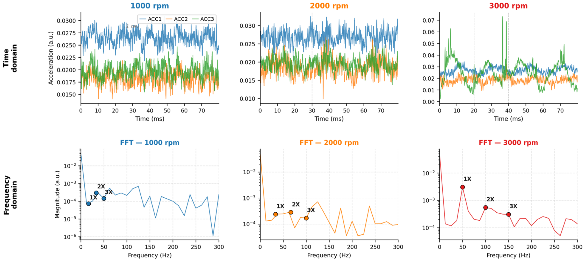
Figure 3.
Vibration signal characteristics at three operating speeds (dynamic unbalance class). Top row: time-domain waveforms (ACC1, ACC2, and ACC3 overlaid). Bottom row: FFT spectra of ACC1 signal (markers indicate 1×, 2×, and 3× harmonics).
Figure 3.
Vibration signal characteristics at three operating speeds (dynamic unbalance class). Top row: time-domain waveforms (ACC1, ACC2, and ACC3 overlaid). Bottom row: FFT spectra of ACC1 signal (markers indicate 1×, 2×, and 3× harmonics).
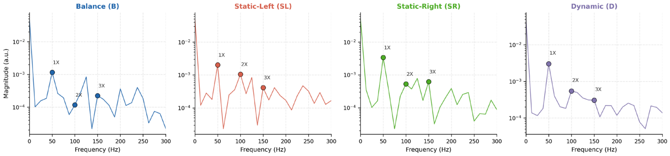
Figure 4.
FFT spectra at 3000 rpm for all four fault classes (ACC1 channel). Markers indicate 1×, 2×, and 3× harmonic frequencies.
Figure 4.
FFT spectra at 3000 rpm for all four fault classes (ACC1 channel). Markers indicate 1×, 2×, and 3× harmonic frequencies.
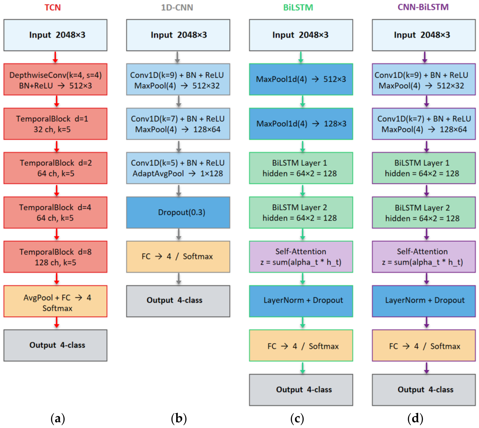
Figure 5.
Architecture diagrams for the four deep learning models. (a) TCN with dilated temporal convolutions. (b) 1D-CNN with three convolutional blocks. (c) BiLSTM with MaxPool downsampling and self-attention. (d) CNN-BiLSTM combining (b,c).
Figure 5.
Architecture diagrams for the four deep learning models. (a) TCN with dilated temporal convolutions. (b) 1D-CNN with three convolutional blocks. (c) BiLSTM with MaxPool downsampling and self-attention. (d) CNN-BiLSTM combining (b,c).
Figure 6.
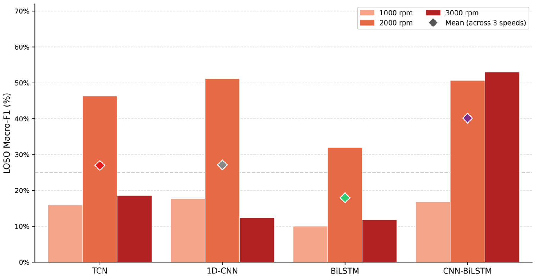
LOSO macro-F1 by model and held-out test speed. Grouped bars: per-speed performance; diamonds: mean F1 across three speeds. Dashed line: chance level (0.250).
Figure 6.
LOSO macro-F1 by model and held-out test speed. Grouped bars: per-speed performance; diamonds: mean F1 across three speeds. Dashed line: chance level (0.250).
Figure 7.
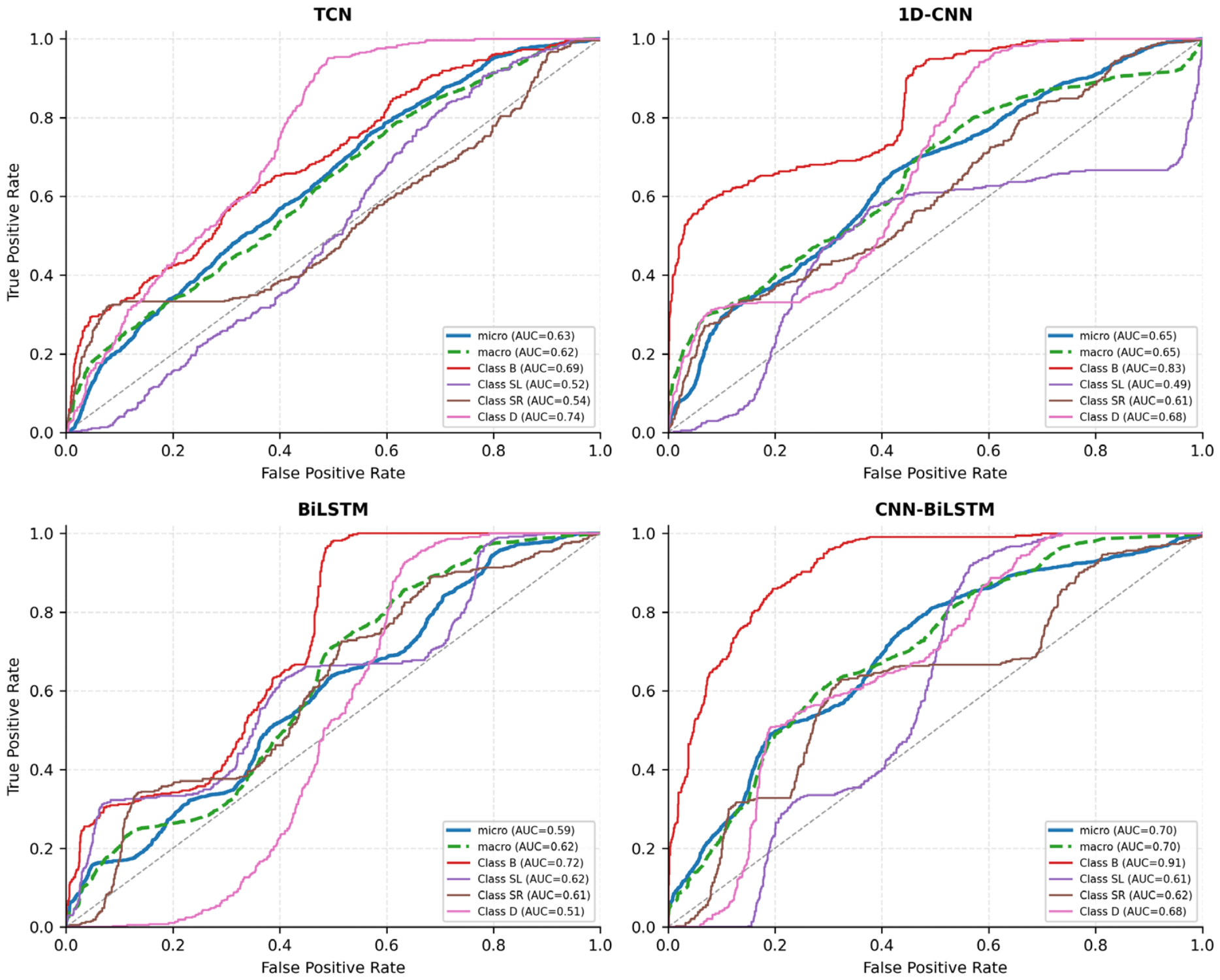
ROC curves for all four models under LOSO evaluation (predictions pooled across three held-out speeds). Macro-AUC: CNN-BiLSTM 0.704, 1D-CNN 0.654, TCN 0.622, BiLSTM 0.616.
Figure 7.
ROC curves for all four models under LOSO evaluation (predictions pooled across three held-out speeds). Macro-AUC: CNN-BiLSTM 0.704, 1D-CNN 0.654, TCN 0.622, BiLSTM 0.616.
Figure 8.
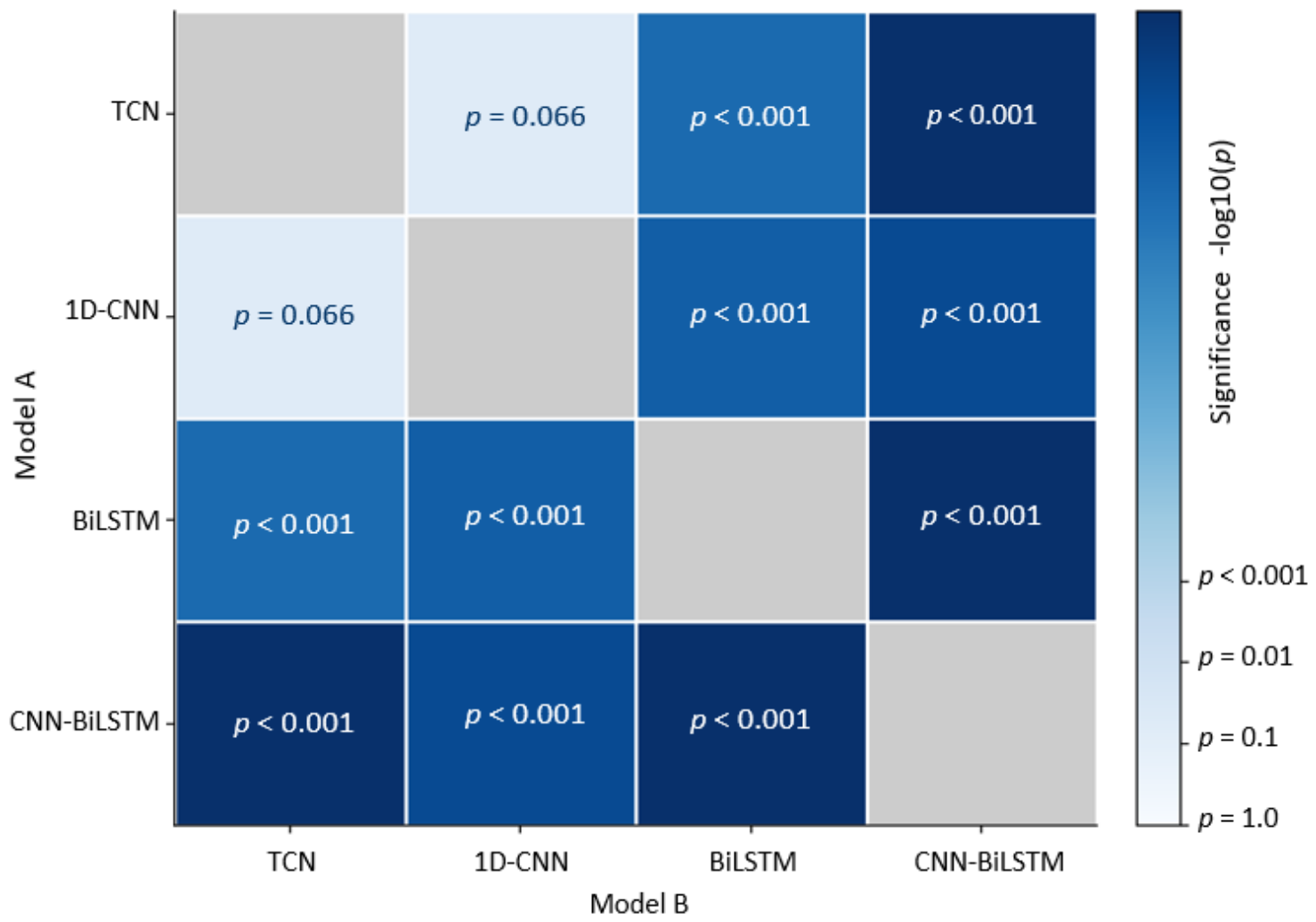
DeLong pairwise AUC significance heatmap. Color encodes −log10(p); darker blue indicates a more significant difference. Diagonal cells (same model) are shown in grey.
Figure 8.
DeLong pairwise AUC significance heatmap. Color encodes −log10(p); darker blue indicates a more significant difference. Diagonal cells (same model) are shown in grey.
Figure 9.
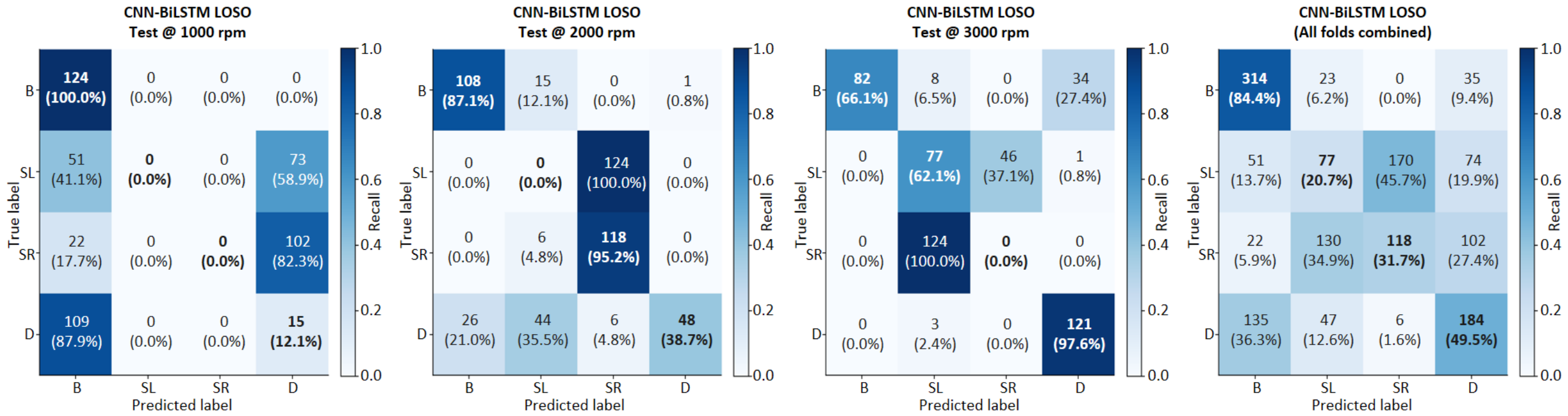
LOSO confusion matrices of CNN-BiLSTM by held-out test speed. Left three panels: per-speed results (1000, 2000, and 3000 rpm); right panel: pooled across all three held-out speeds (the number of windows = 1488). Rows: true class; columns: predicted class.
Figure 9.
LOSO confusion matrices of CNN-BiLSTM by held-out test speed. Left three panels: per-speed results (1000, 2000, and 3000 rpm); right panel: pooled across all three held-out speeds (the number of windows = 1488). Rows: true class; columns: predicted class.
Table 1.
Dataset summary.
Table 1.
Dataset summary.
| Parameter | Value |
|---|
| Total windows | 1488 |
| Window length | 2048 samples (80 ms) |
| Sensor channels | 3 (ACC1, ACC2, ACC3) |
| Sampling frequency (fs) | 25.6 kHz |
| Operating speeds | 1000, 2000, 3000 rpm |
| Fault classes | B (Balance), SL, SR, D |
| Windows per speed | 496 |
| Windows per class | 372 |
| Windows per speed–class pair | 124 |
Table 2.
Within-speed 5-fold cross-validation results at 1000, 2000, and 3000 rpm. All four architectures achieve macro-F1 = 1.0, providing no basis for architecture selection under this protocol.
Table 2.
Within-speed 5-fold cross-validation results at 1000, 2000, and 3000 rpm. All four architectures achieve macro-F1 = 1.0, providing no basis for architecture selection under this protocol.
| Model | 1000 rpm | 2000 rpm | 3000 rpm |
|---|
| Mean F1 | Std F1 | Mean F1 | Std F1 | Mean F1 | Std F1 |
|---|
| TCN | 1.000 | 0.000 | 1.000 | 0.000 | 1.000 | 0.000 |
| 1D-CNN | 1.000 | 0.000 | 1.000 | 0.000 | 1.000 | 0.000 |
| BiLSTM | 1.000 | 0.000 | 1.000 | 0.000 | 1.000 | 0.000 |
| CNN-BiLSTM | 1.000 | 0.000 | 1.000 | 0.000 | 1.000 | 0.000 |
Table 3.
LOSO macro-F1 by model and held-out test speed. CNN-BiLSTM achieves the highest mean LOSO macro-F1 of 0.401. The nominal chance level for a balanced four-class problem is 0.250.
Table 3.
LOSO macro-F1 by model and held-out test speed. CNN-BiLSTM achieves the highest mean LOSO macro-F1 of 0.401. The nominal chance level for a balanced four-class problem is 0.250.
| Model | @1000 rpm | @2000 rpm | @3000 rpm | Mean F1 | Std F1 |
|---|
| BiLSTM | 0.101 | 0.320 | 0.118 | 0.180 | 0.100 |
| TCN | 0.160 | 0.463 | 0.187 | 0.270 | 0.137 |
| 1D-CNN | 0.177 | 0.512 | 0.125 | 0.271 | 0.172 |
| CNN-BiLSTM | 0.168 | 0.507 | 0.530 | 0.401 | 0.165 |
Table 4.
Per-class LOSO macro-F1 scores (fold-averaged across three held-out speeds). CNN-BiLSTM achieves the highest F1 for balance (B) and dynamic (D) fault types. BiLSTM shows near-zero F1 for static right (SR) unbalance and dynamic (D) unbalance, indicating collapse under cross-speed conditions for these fault classes.
Table 4.
Per-class LOSO macro-F1 scores (fold-averaged across three held-out speeds). CNN-BiLSTM achieves the highest F1 for balance (B) and dynamic (D) fault types. BiLSTM shows near-zero F1 for static right (SR) unbalance and dynamic (D) unbalance, indicating collapse under cross-speed conditions for these fault classes.
| Model | F1 | Mean Macro-F1 |
|---|
| Balance | SL | SR | D |
|---|
| BiLSTM | 0.374 | 0.335 | 0.005 | 0.005 | 0.180 |
| TCN | 0.341 | 0.140 | 0.222 | 0.376 | 0.270 |
| 1D-CNN | 0.470 | 0.004 | 0.225 | 0.385 | 0.271 |
| CNN-BiLSTM | 0.737 | 0.153 | 0.212 | 0.505 | 0.401 |
Table 5.
Pairwise DeLong test results (micro-averaged placement values, pooled 1488-sample evaluation set). AUC values are from the DeLong placement statistic and may differ slightly from the macro-AUC values in
Figure 7, which are computed via scikit-learn one-vs.-rest ROC-AUC.
Table 5.
Pairwise DeLong test results (micro-averaged placement values, pooled 1488-sample evaluation set). AUC values are from the DeLong placement statistic and may differ slightly from the macro-AUC values in
Figure 7, which are computed via scikit-learn one-vs.-rest ROC-AUC.
| Comparison | AUC Values | p-Value | Interpretation |
|---|
| CNN-BiLSTM vs. BiLSTM | 0.699 vs. 0.590 | <0.001 | Significant |
| CNN-BiLSTM vs. TCN | 0.699 vs. 0.634 | <0.001 | Significant |
| CNN-BiLSTM vs. 1D-CNN | 0.699 vs. 0.652 | <0.001 | Significant |
| 1D-CNN vs. BiLSTM | 0.652 vs. 0.590 | <0.001 | Significant |
| TCN vs. BiLSTM | 0.634 vs. 0.590 | <0.001 | Significant |
| TCN vs. 1D-CNN | 0.634 vs. 0.652 | 0.066 | Not significant |
Table 6.
Bootstrap 95% confidence intervals (2000 resamples, percentile method) for macro-F1 and macro-AUC under LOSO evaluation. Values in brackets are [lower, upper] of 95% CI bounds. Per-speed F1 CIs are computed within each held-out speed fold independently.
Table 6.
Bootstrap 95% confidence intervals (2000 resamples, percentile method) for macro-F1 and macro-AUC under LOSO evaluation. Values in brackets are [lower, upper] of 95% CI bounds. Per-speed F1 CIs are computed within each held-out speed fold independently.
| Model | Macro-F1 (Pooled) | Macro-AUC (Pooled) | F1 @ 1000 rpm | F1 @ 2000 rpm | F1 @ 3000 rpm |
|---|
| BiLSTM | 0.224 [0.210, 0.237] | 0.616 [0.598, 0.635] | 0.101 [0.088, 0.113] | 0.320 [0.296, 0.344] | 0.118 [0.105, 0.132] |
| TCN | 0.363 [0.338, 0.386] | 0.623 [0.604, 0.642] | 0.160 [0.137, 0.184] | 0.463 [0.427, 0.495] | 0.187 [0.159, 0.213] |
| 1D-CNN | 0.331 [0.311, 0.352] | 0.654 [0.634, 0.672] | 0.177 [0.155, 0.201] | 0.512 [0.479, 0.543] | 0.125 [0.105, 0.145] |
| CNN-BiLSTM | 0.443 [0.420, 0.467] | 0.704 [0.690, 0.717] | 0.168 [0.149, 0.187] | 0.507 [0.474, 0.536] | 0.530 [0.501, 0.558] |
Table 7.
Variation in centrifugal force with different rotational speeds.
Table 7.
Variation in centrifugal force with different rotational speeds.
| Speed | ω (Rad/s) | F = meω2 | Relative Scale |
|---|
| 1000 rpm | 104.7 | 5.3 N | 1× |
| 2000 rpm | 209.4 | 21.1 N | 4× |
| 3000 rpm | 314.2 | 47.5 N | 9× |




 ,
,