Time Is of the Essence: A Comparative Study of Continuous (NCDE) and Discrete (LSTM) Time Models for User Anomaly Detection

Abstract

User Behaviour Analytics (UBA) relies heavily on sequential data to detect anomalies such as insider threats. Traditional approaches often model user behaviour as discrete sequences of events using Recurrent Neural Networks (RNNs) like Long Short-Term Memory (LSTM) networks. These methods implicitly treat time steps as uniform, ignoring the irregular time intervals inherent in user logs. In this paper, we present the first application of Neural Controlled Differential Equations (NCDEs) to user behaviour analytics, a class of continuous-time models that naturally handle irregularly-timed event data. We compare a simple LSTM predictor against an NCDE predictor on the CERT 4.2 and 6.2 insider threat dataset. We demonstrate that standard discrete-time models (LSTMs) produce noisy loss signals on sparse data, forcing downstream classifiers to rely on fragile error spikes. In contrast, Neural CDEs generate stable, continuous error signals. NCDE roughly tripled the F1 of the discrete baseline (0.364 vs. 0.133) on the challenging CERT 6.2 dataset.

1. Introduction

User behaviour analytics (UBA) is a critical component of modern cybersecurity, particularly for detecting insider threats and account takeovers. The volume of log data generated by modern enterprises necessitates automated approaches, leading to the widespread adoption of machine learning.

Traditional deep learning approaches model user behaviour as a discrete sequence of events. Methods like Hidden Markov Models (HMM) and Long Short-Term Memory (LSTM) networks process inputs step-by-step, implicitly assuming that the duration between event t and event $t+1$ is irrelevant or uniform. These methods typically ignore the time intervals between events, which can contain valuable information about user behaviour. In real-world cybersecurity logs, time can be and usually is highly irregular. A user might generate a burst of 50 events in one minute or even second (e.g., script execution) and then be inactive for hours or days.

In this paper, we compare a widely used discrete LSTM approach against Neural Controlled Differential Equations (NCDEs). NCDEs treat the data not as a sequence of discrete steps, but as a continuous path derived from the input, controlled by a differential equation. We hypothesise that by utilising a model designed for continuous time, we can achieve superior anomaly detection performance. We test this on the CERT dataset, comparing an LSTM predictor against an NCDE predictor. Furthermore, we investigate the specific impact of “time” by analysing whether the use of real timestamps versus interpolated steps affects the model’s discriminative power.

Related Work

The field of user behaviour analytics has a rich history, with a wide variety of methods being applied to the problem of anomaly detection. The CERT insider threat dataset, first introduced in 2013 by [1], remains the standard benchmark for this domain due to its realistic simulation of insider threat scenarios. A comprehensive survey of UBA and Account Takeover (ATO) research by [2] provides a broad overview of the state of the art in this field. Research using the CERT dataset has evolved from traditional machine learning methods to complex deep learning architectures, but most existing approaches share a common dependency on discrete-time modelling.

Early work on this dataset often employed traditional machine learning models such as Hidden Markov Models (HMMs). Ref. [3] utilised Hidden Markov Models (HMMs), which represent user behaviour as a set of states and transition probabilities. While HMMs are effective for capturing short-term dependencies, they can sometimes struggle with the long-term context required to detect sophisticated insider threats that unfold over weeks or months.

Various decision tree-based approaches are also often applied, in particular Random Forest approaches for supervised classification [4,5] or Isolation Forest [6,7] as one of the most commonly used unsupervised approaches.

Bayesian methods have also been explored to model the probability of user actions due to their computational simplicity and explainability, either as a benchmark method or as part of an ensemble [8,9]. However, these approaches often rely on manual feature engineering and may fail to capture complex non-linear patterns in user activity.

As computational power increased, the field rapidly shifted toward deep learning to capture these non-linear complexities and long-range dependencies. Ref. [10] were among the first to apply LSTMs to the CERT dataset. They demonstrated that LSTMs could capture long-range dependencies in user behaviour that simple Markovian models missed. Their work established the “next-event prediction” paradigm, where the model learns to predict the next user action, and high prediction error indicates an anomaly.

This was followed by the introduction of the LSTM autoencoder by [11], which focused on reconstruction error rather than prediction error. Ref. [12] further extended this by combining LSTM autoencoders with Generative Adversarial Networks (GANs) to handle the extreme class imbalance inherent in the dataset.

While effective, these methods share a common limitation: they are discrete-time models. They ingest sequences of events (e.g., ‘[Logon, File_Access, Email]’) and treat the step from ‘Logon’ to ‘File_Access’ as identical to the step from ‘File_Access’ to ‘Email’, regardless of whether the time difference was 1 s or 1 h. This discretisation discards potentially valuable temporal information. There are various approaches with encoding the time component directly into events, producing e.g., ‘Logon_working_hours’ or ‘Logon_night’, as well as putting the events into hourly buckets but, as to our best knowledge, there are no approaches using continuous time as a model input.

While variations like Time-LSTM, as described by [13], attempt to handle irregular intervals by modifying the forget gates with time decay, they fundamentally remain discrete-time models. They still rely on discrete updates and may struggle to capture the continuous latent dynamics of user behaviour as effectively as a native differential equation solver.

Neural Controlled Differential Equations (NCDEs), introduced by [14], offer a mathematically rigorous solution to irregular time series. Unlike RNNs, which update hidden states at discrete steps, NCDEs define the hidden state $z\left(t\right)$ as the solution to an Ordinary Differential Equation (ODE) controlled by the continuous data path $X\left(t\right)$:

$$dz\left(t\right)=f_{\theta }\left(z\left(t\right)\right)dX\left(t\right)$$

(1)

This allows the model to naturally handle missing data and irregular timestamps without imputation. While NCDEs have shown state-of-the-art performance in medical [15,16], physics [17] or chemistry [18] time series (where irregular sampling is common), to the best of our knowledge, this work represents the first application of NCDEs to the CERT insider threat dataset. This paper bridges the gap by directly comparing the discrete LSTM baseline against the continuous NCDE approach on the same feature sets.

2. Materials and Methods

The CERT dataset, although introduced in 2013, still remains one of the most used datasets for testing new machine learning approaches in the field. The dataset has multiple revisions, with versions 4.2 and 6.2 accounting for the vast majority of usage in literature.

2.1. Data Preparation

Both revisions of the dataset consist of the same set of files, with a difference in the size and number of injected insiders, seventy for version 4.2 and just five, one per scenario, in version 6.2.

Version 4.2 of the dataset simulates a company or a government agency of 1000 employees over 17 months, with 70 insiders (30 for scenario 1 and 2, 10 for scenario 3) and is considered a dense-needle dataset. User events are saved as lines in CSV files, as displayed in

Table 1. Cert 4.2  files.

File	Fields	Number of Rows	Size
logon.csv	id, date, user, pc, activity	854,860	58.5 M
http.csv	id, date, user, pc, url, content	28,434,424	14.5 G
file.csv	id, date, user, pc, filename, content	445,582	193.1 M
device.csv	id, date, user, pc, activity	405,381	29 M
email.csv	id, date, user, pc, to, cc, bcc, from, size, attachments, content	2,629,980	1.4 G
psychometric.csv	employee_name, user_id, O, C, E, A, N	1000	44 K

. Insider events are manually injected, and only 0.03% of the events are categorised as malicious in the CERT 4.2 dataset, while CERT 6.2 pushes this further with malicious events comprising only 0.00035% of the dataset (470 malicious events out of 135 million total events). This extreme class imbalance poses a significant challenge for traditional classifiers and requires metrics like PR-AUC and F1 to complement the standard AUC-ROC, making accuracy completely unusable in this context.

Version 6.2 of the dataset depicts a company or a government agency of 4000 employees over 17 months. User events are provided in the CSV files, as shown in

Table 2. Cert 6.2 files.

Filename	Fields	Number of Rows	Size
device.csv	id, date, user, pc, file_tree, activity	1,551,828	139 M
email.csv	id, date, user, pc, to, cc, bcc, from, activity, size, attachments, content	10,994,957	8.1 G
file.csv	id, date, user, pc, filename, activity, to_removable_media, from_removable_media, content	2,014,883	1.3 G
http.csv	id, date, user, pc, url, activity, content	117,025,216	92.1 G
logon.csv	id, date, user, pc, activity	3,530,285	241.6 M
psychometric.csv	employee_name, user_id, O, C, E, A, N	4000	185 K

.

Table 3. CERT scenarios ¹.

Scenario	Description	4.2	6.2
1	User who did not previously use removable drives or work after hours begins logging in after hours, using a removable drive, and uploading data to wikileaks.org. Leaves the organisation shortly thereafter.	30	1
2	User begins surfing job websites and soliciting employment from a competitor. Before leaving the company, they use a thumb drive (at markedly higher rates than their previous activity) to steal data.	30	1
3	System administrator becomes disgruntled. Downloads a keylogger and uses a thumb drive to transfer it to his supervisor’s machine. The next day, he uses the collected keylogs to log in as his supervisor and send out an alarming mass email, causing panic in the organisation. He leaves the organisation immediately.	10	1
4	A user logs into another user’s machine and searches for interesting files, emailing them to their home email. This behaviour occurs more and more frequently over a 3-month period.	–	1
5	A member of a group decimated by layoffs uploads documents to Dropbox, planning to use them for personal gain.	–	1

¹ Source: [19].

shows brief scenario descriptions; as defined by [1], version 4.2 contains scenarios 1–3, while version 6.2 contains all five scenarios.

In our experiments, we used the complete CERT 4.2 dataset. For CERT 6.2, due to its prohibitive size, we followed an established convention in the literature by randomly selecting a subset of 500 users, similar to [20] or [21]. This selection was performed using a fixed random seed (42) to ensure complete reproducibility, while manually ensuring the inclusion of all 5 malicious insiders. While the sampling was purely random rather than explicitly stratified by user activity or department, an analysis of the resulting subset confirms it is highly representative of the broader CERT 6.2 population. Due to the severe computational bottleneck of the NCDE adaptive step-size solver, which requires approximately 20 h of training and scoring time per run, conducting multiple rounds of k-fold sampling was computationally prohibitive. However, as demonstrated in

Table 4. CERT 6.2 Department distribution: original vs. sampled population.

Department	Original Population (%)	Sampled Population (%)
Engineering	32.8% (1311)	32.0% (160)
Assembly	18.1% (725)	17.8% (89)
Software Management	12.2% (489)	11.8% (59)
Field Service	9.4% (378)	10.2% (51)
Research	8.5% (342)	10.4% (52)
Sales	9.4% (378)	7.8% (39)
Security	5.4% (219)	6.2% (31)
Other	4.2% (168)	3.8% (19)

, the demographic alignment between the original dataset and our sample confirms the absence of significant sampling bias, providing confidence in the stability and generalizability of our baseline. The code for subset generation is available in the Zenodo repository accompanying this paper [22].

Following the methodology of [3], we extracted two feature sets to test the models’ sensitivity to feature engineering, and then aggregated events by user and week:

• Simple: 7 basic events
• Comprehensive: 16 events encoding week-day and working-hour distinctions

The full event table is shown in

Table 5. CERT extracted feature variants.

Simple	Comprehensive
logon	weekday_logon
logoff	weekday_logon_afterhours
connect	weekend_logon
disconnect	logoff
email	file_exe
http	file_jpg
file	file_zip
	file_txt
	file_doc_pdf
	internal_email
	external_email
	weekday_connect
	weekday_connect_afterhours
	weekend_connect
	disconnect
	website

.

2.2. Model Architectures

We employ a two-stage self-supervised approach. The core sequence models (LSTM/NCDE) were trained in a purely self-supervised manner (next-event prediction) without exposure to anomaly labels. For the evaluation phase, we utilise the generated error signals as features for a downstream classifier to quantify the distinctiveness of the learned representations rather than to train the anomaly model itself.

The main ideas are to test if the added temporal information in the comprehensive variant helps LSTM to better differentiate between the classes and to test if the complete temporal information helps NCDE. Since the dataset contains no insider attacks in the first twenty weeks, they are used for training a global model per method and variant; afterwards, each user’s week is scored.

This setup, using global models and anomaly detection, is performed in order to simulate a real-world scenario where labels are either non-existent or scarce and where training a model per user for millions of users is impractical.

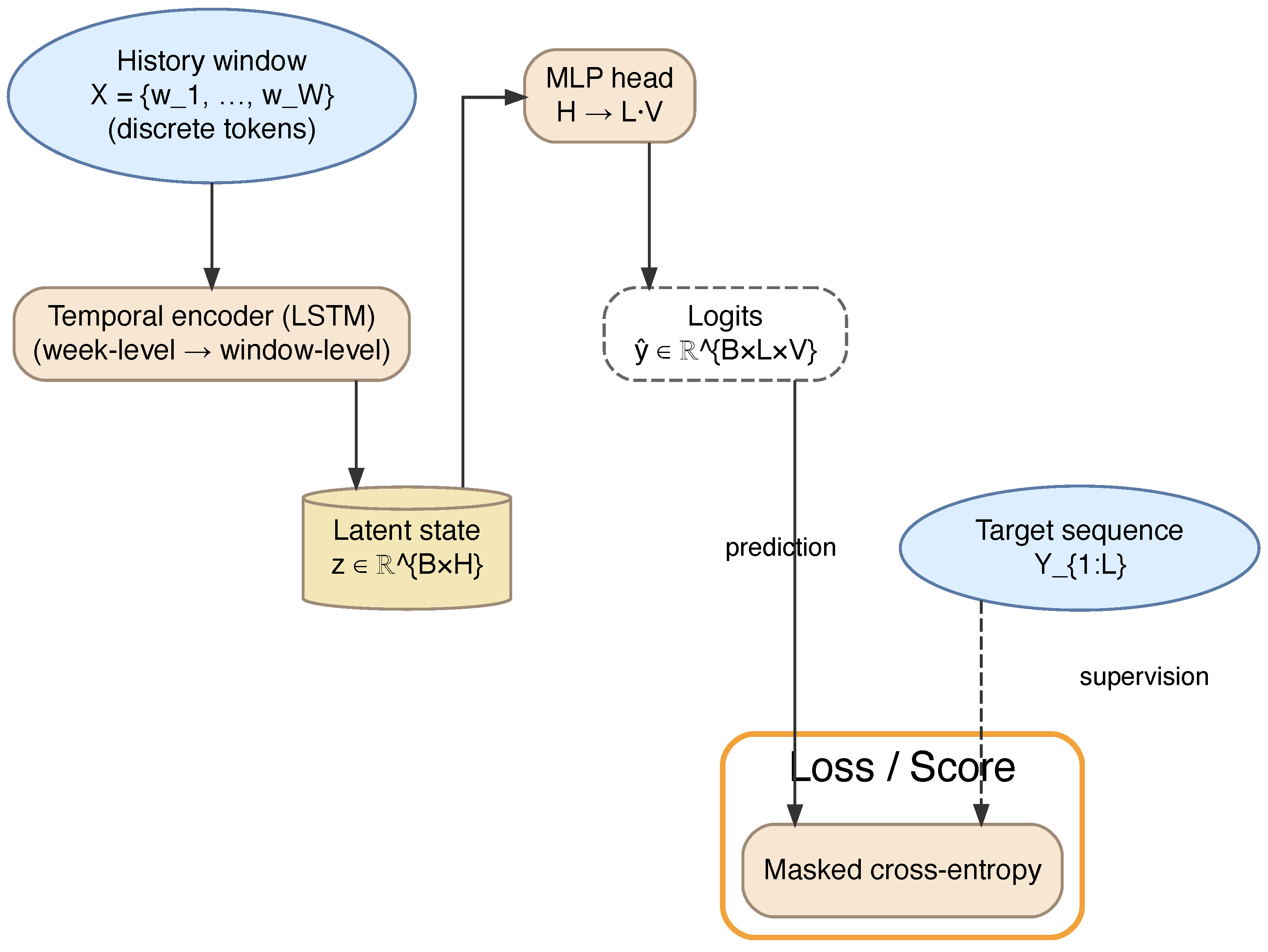
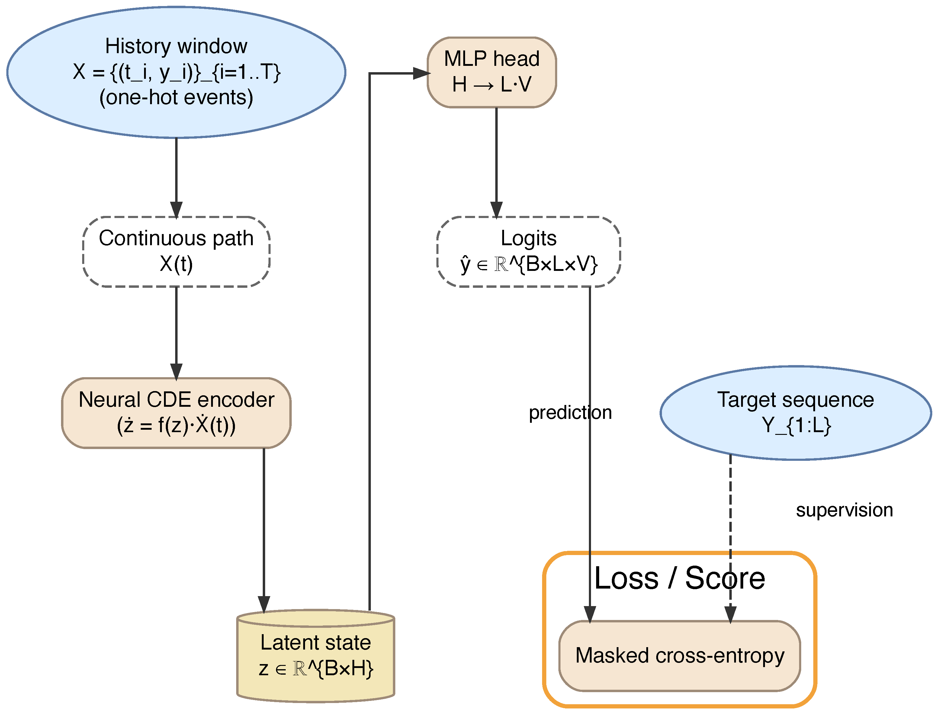
To provide a rigorous comparison between continuous and discrete paradigms and compare the models on equal terms, the capacity and architecture were matched, as shown in Figure 1 and Figure 2; the full hyperparameter table is provided in Appendix A.

2.2.1. LSTM Predictor

Our baseline is a hierarchical LSTM architecture designed for discrete event sequences. The model receives a history window $W_{hist}$ of k previous weeks.

• A shared encoder (Embedding layer + Bidirectional LSTM) maps each week’s discrete events to a fixed dense vector h.
• The sequence of history vectors is processed by a second unidirectional LSTM to summarise the user’s recent temporal history.
• A fully connected MLP projects the final hidden state to output the logits for the sequence of action tokens in the next week $t+1$.
• The model is trained to minimise the Cross-Entropy Loss between the predicted token probability distributions and the actual next-week actions.

The architecture of the LSTM model is shown in Figure 1 and can be formally described as follows:

Input Representation

The history window consists of W weekly sequences,

$$X=\{X_1,\dots ,X_W\},X_w=(x_{w,1},\dots ,x_{w,T_w}),$$

(2)

where $x_{w,t}\in \{1,\dots ,V\}$ denotes a discrete event token.

Each token is mapped to an embedding vector using a learned embedding matrix E:

$$e_{w,t}=E\left(x_{w,t}\right)\in {\mathbb{R}}^d.$$

(3)

Hierarchical Encoder Structure

The encoder operates hierarchically, first processing the high-frequency events within each week, and subsequently aggregating these weekly summaries into a global history vector.

Week-Level Encoding

Each week w consists of a sequence of discrete event tokens. Unlike the simplified recurrent formulation often presented in high-level overviews, our baseline utilises a standard Long Short-Term Memory (LSTM) cell to mitigate the vanishing gradient problem. For a given week w, the update mechanism at step t processes the input embedding $e_{w,t}$ and the previous hidden state $h_{t-1}$ through a series of gating mechanisms:

$$\begin{array}{cc}\hfill f_t& =\sigma (W_f·[h_{t-1},e_{w,t}]+b_f)\hfill \\ \hfill i_t& =\sigma (W_i·[h_{t-1},e_{w,t}]+b_i)\hfill \\ \hfill {\tilde{C}}_t& =tanh(W_C·[h_{t-1},e_{w,t}]+b_C)\hfill \\ \hfill C_t& =f_t\odot C_{t-1}+i_t\odot {\tilde{C}}_t\hfill \\ \hfill o_t& =\sigma (W_o·[h_{t-1},e_{w,t}]+b_o)\hfill \\ \hfill h_t& =o_t\odot tanh\left(C_t\right)\hfill \end{array}$$

(4)

Here, $\sigma$ denotes the sigmoid activation function, and ⊙ represents the Hadamard product. The forget gate $f_t$ is particularly relevant to our comparison; it determines how much of the previous cell state $C_{t-1}$ is retained. In this discrete formulation, the transition from $t-1$ to t implies a uniform “computational step”, ignoring the actual time elapsed between log events. The final hidden state of this sequence forms the week representation:

$$h^{\left(w\right)}=h_{T_w}\in {\mathbb{R}}^D$$

(5)

Window-Level Encoding

Once the sequence of weeks is encoded into a set of vectors $H=(h^{\left(1\right)},\dots ,h^{\left(W\right)})$, a second, unidirectional LSTM layer aggregates the history window. This layer captures the long-term evolution of the user’s behaviour over the k previous weeks:

$$z={\mathrm{LSTM}}_{window}\left(H\right)\in {\mathbb{R}}^{H_{dim}}$$

(6)

The final hidden state z serves as the compressed latent representation of the user’s entire history window, which is then passed to the prediction head.

Prediction Head

The latent state is decoded using a feedforward network:

$$\widehat{Y}=\mathrm{MLP}\left(z\right)\in {\mathbb{R}}^{L\times V}.$$

(7)

The predictive distribution at each position is given by

$${\widehat{p}}_{\theta }(y_{\ell }\mid X)=\mathrm{Softmax}\left({\widehat{Y}}_{\ell }\right).$$

(8)

Training Objective

Let $m_{\ell }\in \{0,1\}$ indicate whether position ℓ is valid (non-padding). The model is trained by minimising the masked cross-entropy loss

$${\mathcal{L}}_{\mathrm{LSTM}}\left(\theta \right)={\displaystyle \frac{1}{{\sum }_{\ell =1}^L{m}_{\ell }}}{\displaystyle \sum _{\ell =1}^L}{m}_{\ell }\mathrm{CE}\left({\widehat{p}}_{\theta }(y_{\ell }\mid X),y_{\ell }\right).$$

(9)

2.2.2. NCDE Predictor

The NCDE predictor transforms the discrete sequence into a continuous path to control the neural differential equation.

• Path Construction: The sequences of events in the history window are concatenated into a single stream. The discrete events are transformed into a continuous path $X\left(t\right)$ via linear interpolation. To preserve the temporal density and velocity of user actions, we employ an Elapsed Time formulation:
  • Timestamps are calculated as elapsed hours since the start of the window.
  • These values are scaled by a fixed global constant (e.g., the maximum window duration) to the range $[0,1]$. Unlike min–max normalisation, this preserves the relative gaps between events, allowing the ODE solver to distinguish between rapid bursts of activity and sparse interactions.
• Neural CDE: The path $X\left(t\right)$ controls the evolution of the latent state $z\left(t\right)$ via the equation $dz\left(t\right)=f_{\theta }\left(z\left(t\right)\right)dX\left(t\right)$. To compute the terminal latent state $z\left(1\right)$, we numerically solve this equation using an adaptive step-size solver. This allows the model to maintain high integration precision during rapid bursts of activity (e.g., script execution) while remaining computationally efficient during long periods of inactivity. The vector field $f_{\theta }$ was dimensioned to ensure the total parameter count matches the baseline LSTM (≈400 k parameters) for architectural parity.
• Prediction: The final latent state $z\left(T\right)$ is projected via an MLP to output a probability distribution (logits) over the user states for the target sequence. The model is optimised using Softmax Cross-Entropy loss, treating the anomaly detection task as a classification problem comparable to the discrete baseline.

The architecture is shown in Figure 2 and can be formally described as follows:

Continuous Path Construction

The core advantage of the Neural CDE lies in its ability to decouple the observation times from the model’s internal dynamics. To achieve this, the discrete sequence of user events $X={\left\{(t_i,y_i)\right\}}_{i=1}^T$ must be lifted into a continuous path $X\left(t\right)$.

While NCDEs natively support higher-order path interpolation, such as cubic splines, we intentionally employed linear interpolation for all reported experiments. Preliminary testing has shown that while cubic splines offer increased smoothness, they also introduce significant computational overhead and numerical instability within the adaptive ODE solver during training. Linear interpolation has provided the optimal balance between preserving the temporal velocity of user actions and ensuring numerical convergence.

The path is defined as $X\left(t\right):[0,T_{max}]\to {\mathbb{R}}^V$. For the linear case, the path between two observed events at times $t_i$ and $t_{i+1}$ is defined explicitly as

$$X\left(t\right)=X_{t_i}+{\displaystyle \frac{X_{t_{i+1}}-X_{t_i}}{t_{i+1}-t_i}}(t-t_i)\mathrm{for}t\in [t_i,t_{i+1}]$$

(10)

This continuous path $X\left(t\right)$ serves as the driving signal for the differential equation. Unlike the discrete LSTM, which “jumps” from state to state, the NCDE solver integrates along this path. Consequently, if the time gap $t_{i+1}-t_i$ is large (e.g., a weekend of inactivity), the latent state $z\left(t\right)$ continues to evolve according to the vector field dynamics, allowing the model to naturally encode the duration of inactivity without requiring explicit “time-decay” heuristics.

Encoder (Neural CDE)

• Initial state

The latent state is initialised via a learnable map

$$z\left(0\right)=g_{\theta }\left(X\left(0\right)\right),g_{\theta }:{\mathbb{R}}^V\to {\mathbb{R}}^H.$$

(11)

• Latent dynamics

The latent state evolves according to a controlled differential equation

$${\displaystyle \frac{dz\left(t\right)}{dt}}=f_{\theta }\left(z\left(t\right)\right){\displaystyle \frac{dX\left(t\right)}{dt}},$$

(12)

where

$$f_{\theta }:{\mathbb{R}}^H\to {\mathbb{R}}^{H\times V}$$

(13)

is a neural vector field.

• Final state

The latent representation is defined as the terminal value

$$z=z\left(1\right),$$

(14)

obtained by numerically solving the CDE from $t=0$ to $t=1$.

Prediction Head

As in the LSTM model, the latent state is decoded by a feedforward network:

$$\widehat{Y}=\mathrm{MLP}\left(z\right)\in {\mathbb{R}}^{L\times V},$$

(15)

with predictive distribution

$${\widehat{p}}_{\theta }(y_{\ell }\mid X)=\mathrm{Softmax}\left({\widehat{Y}}_{\ell }\right).$$

(16)

Training Objective

Using the same masking convention $m_{\ell }\in \{0,1\}$, the Neural CDE model is trained by minimizing

$${\mathcal{L}}_{\mathrm{NCDE}}\left(\theta \right)={\displaystyle \frac{1}{{\sum }_{\ell =1}^L{m}_{\ell }}}{\displaystyle \sum _{\ell =1}^L}{m}_{\ell }\mathrm{CE}\left({\widehat{p}}_{\theta }(y_{\ell }\mid X),y_{\ell }\right).$$

(17)

2.2.3. Implementation Details

Pytorch [23] (version 2.7.1) was used for LSTM approach, and for NCDE, a jit compiled version using the JAX framework [24] (version 0.5.3) and diffrax [14] (version 0.7.0), using an adaptive step-size solver were utilised.

The entire experiment and evaluation code is available on Zenodo [22].

All experiments were performed on a prosumer workstation: AMD Ryzen 9 9900X 12-Core CPU, 64 GB of RAM and Nvidia 4070 TI Super with 16 G of RAM. The operating system used was Linux Mint 22.1 with CUDA SDK v12.8, pytorch 2.7.1, jax 0.5.3, equinox 0.13.2 and diffrax 0.7.0.

3. Results

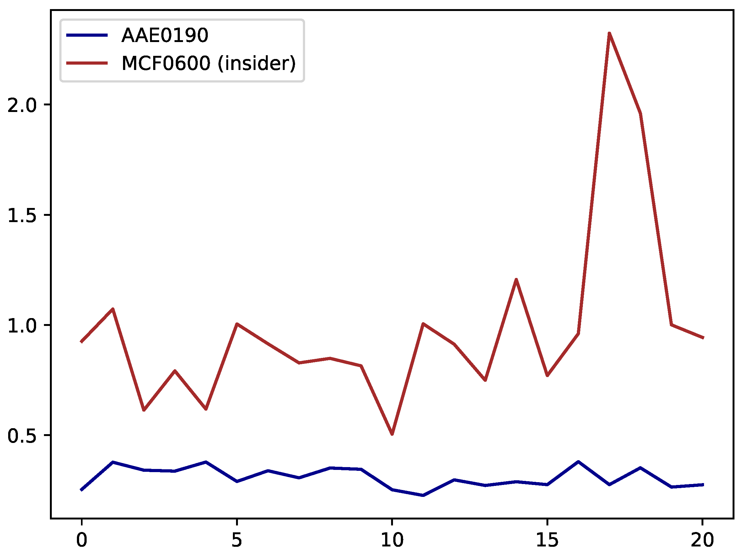
After model training and scoring of users, the results were saved into a file for repeated evaluation experiments. In the ideal case, the anomaly is discernible as a spike in the week scores, as shown in Figure 3, which compares scores of an insider (MCF0600) with a random normal user (AAE0190).

The training and scoring times differed greatly, with LSTM generally being an order of magnitude faster—with both training and scoring being performed in about 2 h, while NCDE training and scoring took almost 20 h on the CERT 4.2 dataset. The NCDE solver also occasionally encountered non-deterministic execution halts despite the availability of system resources. These interruptions, likely stemming from numerical instabilities or stiffness encountered by the adaptive step-size solver during high-velocity event bursts, were mitigated by resuming the process from the specific user, which ultimately allowed for successful completion.

We evaluated all per-user anomaly scores using two families of detectors: classifier-free statistical thresholding applied directly to the raw weekly error signal (per-user Z-score and IQR), and learned binary classifiers trained on features derived from the sorted weekly losses (logistic regression, random forest, and gradient boosting). This dual evaluation directly addresses the concern that a single downstream classifier could bias the LSTM-versus-NCDE comparison.

The classifier-free thresholding methods separated malicious users only weakly on the sparse CERT 6.2 data (PR-AUC near the 0.01 prevalence baseline, as shown in

Table 6. Detection performance (F1 and AUC) across downstream classifiers and raw-signal thresholding. Bold marks the best method within each classifier/dataset/feature-set cell. Z-score and IQR threshold the raw weekly error signal directly (no classifier).

			Z-Score		IQR		LR		RF		XGBoost
Data	Feat.	Method	F1	AUC	F1	AUC	F1	AUC	F1	AUC	F1	AUC
4.2	Simple	LSTM	0.228	0.710	0.231	0.710	0.782	0.983	0.798	0.984	0.838	0.987
4.2	Simple	NCDE	0.208	0.661	0.228	0.691	0.701	0.973	0.772	0.982	0.739	0.980
4.2	Compr.	LSTM	0.237	0.714	0.239	0.724	0.765	0.983	0.800	0.984	0.832	0.984
4.2	Compr.	NCDE	0.216	0.668	0.231	0.694	0.697	0.974	0.798	0.982	0.747	0.978
6.2	Simple	LSTM	0.095	0.663	0.095	0.668	0.286	0.384	0.222	0.636	0.125	0.565
6.2	Simple	NCDE	0.036	0.568	0.113	0.703	0.174	0.715	0.250	0.740	0.250	0.766
6.2	Compr.	LSTM	0.047	0.667	0.056	0.702	0.308	0.548	0.190	0.734	0.133	0.628
6.2	Compr.	NCDE	0.042	0.609	0.082	0.708	0.118	0.571	0.250	0.732	0.364	0.775

and

Table 7. Detection performance (PR-AUC) across downstream classifiers and raw signal thresholding. PR-AUC is the primary metric under the severe class imbalance of CERT 6.2 (5 malicious users). Bold marks the best method within each cell. (See Table 8 for Time-LSTM ablation results).

Data	Feat.	Method	Z-Score	IQR	LR	RF	XGBoost
4.2	Simple	LSTM	0.135	0.141	0.765	0.719	0.760
4.2	Simple	NCDE	0.160	0.169	0.609	0.724	0.694
4.2	Compr.	LSTM	0.132	0.138	0.773	0.708	0.705
4.2	Compr.	NCDE	0.147	0.167	0.662	0.712	0.695
6.2	Simple	LSTM	0.028	0.029	0.107	0.062	0.030
6.2	Simple	NCDE	0.015	0.037	0.050	0.119	0.094
6.2	Compr.	LSTM	0.019	0.023	0.090	0.053	0.034
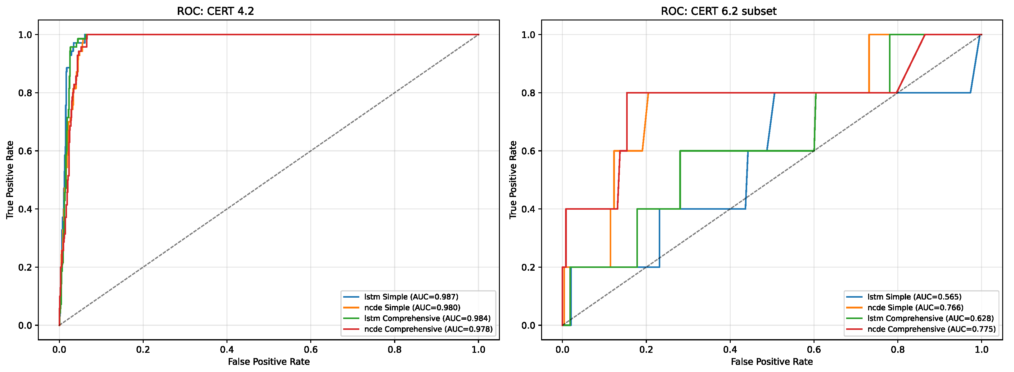
6.2	Compr.	NCDE	0.018	0.033	0.036	0.105	0.288

), indicating that the raw error signal alone is insufficient and that a learned aggregation of the per-week scores is needed. Among the learned classifiers, gradient boosting (XGBoost) gave the strongest detection on 6.2, reaching F1 = 0.364, AUC = 0.775, and PR-AUC = 0.288 for NCDE on the Comprehensive feature set—the latter roughly an order of magnitude above the prevalence baseline and far above the corresponding LSTM result (PR-AUC = 0.034).

The comparison is consistent across classifiers but differs sharply by dataset. On CERT 6.2, NCDE outperforms LSTM under every learned classifier (e.g., random forest: AUC 0.740 vs. 0.636 on Simple), confirming the advantage is not an artefact of the XGBoost choice. On the larger, less imbalanced CERT 4.2 (70 malicious users), the two models are competitive, and LSTM is in fact marginally stronger under the learned classifiers (e.g., XGBoost AUC 0.987 vs. 0.980, Simple), regardless of feature set. Full per-classifier results are given in Table 6 and Table 7, and ROC curves are shown in Figure 4. An ablation study evaluating Time-LSTM (LSTM + explicit temporal modelling) is presented separately in

Table 8. Ablation on CERT 6.2: effect of temporal modelling. LSTM has no explicit time; Time-LSTM adds an inter-event time gate to the LSTM encoder; NCDE models the activity as a continuous-time path. Bold marks the best value per metric within a feature set. Adding time sharply improves ranking (AUC: 0.628 → 0.846), but the continuous-time NCDE extracts a far cleaner positive signal under the 5-positive class imbalance (PR-AUC: 0.288 vs. 0.044), which is the operationally relevant metric.

Feature Set	Method	F1	AUC	PR-AUC
Simple	LSTM	0.133	0.565	0.030
	Time-LSTM	0.133	0.549	0.031
	NCDE	0.250	0.766	0.094
Comprehensive	LSTM	0.133	0.628	0.034
	Time-LSTM	0.105	0.846	0.044
	NCDE	0.364	0.775	0.288

.

4. Discussion

4.1. Continuous vs. Discrete Modelling

Our experiments confirm the hypothesis that continuous-time modelling offers a performance advantage. Although both models achieved comparable results on the “easy”, dense needle 4.2 dataset, the NCDE performed better on the more sparse 6.2 dataset. On CERT 6.2, the NCDE achieved an AUC of 0.775against the LSTM’s 0.628, and a markedly higher PR-AUC (0.288 vs. 0.034), indicating better precision–recall balance, the metric that matters most under this dataset’s extreme imbalance, indicating a better balance of precision and recall, which is crucial for reducing false positives in security operations.

The disparity of AUC and F1 score mirrors the imbalanced nature of the dataset. This highlights a common phenomenon in threat detection: The model succeeds in ranking anomalous weeks higher than most normal weeks (as shown by the AUC), but the sheer volume of normal activity makes precise thresholding difficult. This pattern is reflected in the F1 score, where the NCDE roughly tripled the discrete baseline on 6.2-Comprehensive (0.364 vs. 0.133): by producing a cleaner separation between anomalous and normal weeks, the continuous-time model yields more usable operating points than the discrete LSTM, whose diffuse error signal makes precise thresholding difficult.

This performance gap highlights the limitations of imposing a rigid, discrete grid on naturally fluid user behaviour. By allowing the latent state to evolve continuously between observations, the NCDE captures nuances that the LSTM’s discrete updates miss, even with the provided time information within the comprehensive variant.

To test whether the gap was merely the LSTM’s lack of explicit time awareness, we performed an ablation with Time-LSTM on CERT 6.2. Adding an explicit time gate did improve ranking over the discrete baseline (AUC 0.628 to 0.846 on the Comprehensive feature set), confirming that temporal information is valuable. However, Time-LSTM did not translate this into precise detection under severe class imbalance: its PR-AUC (0.044) remained far below the NCDE’s (0.288), and close to the discrete LSTM (0.034). This indicates that discretely augmenting an LSTM with time intervals is insufficient; the continuous-time formulation is what yields a cleanly separable positive signal.

While many existing approaches to the CERT dataset employ data balancing techniques such as SMOTE [25] to address extreme sparsity, our work shows that continuous-time modelling can offer a robust alternative. By leveraging the NCDE’s ability to maintain a stable latent state across irregular intervals, the model can successfully capture meaningful representations of anomalous behavior.

4.2. Case Study: The Anatomy of a Detection (User MBG3183)

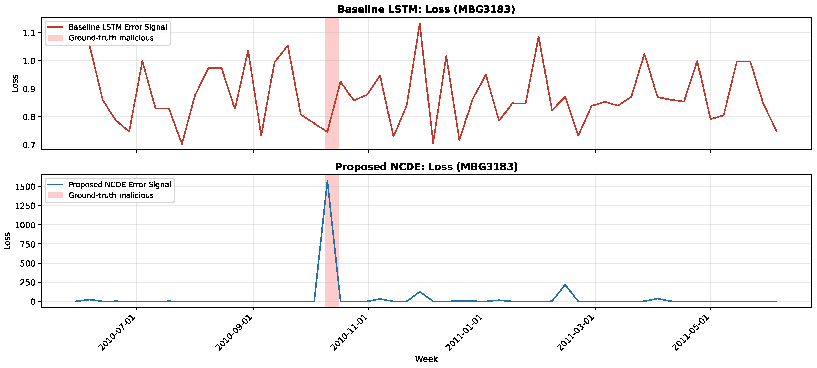
To qualitatively illustrate the difference in error-signal behavior between the two models, we examine the detection timeline for user MBG3183 (CERT Scenario 5, Intellectual Property Theft), whose labelled malicious activity occurs in only four events, all on 12th October 2010. As shown in Figure 5, the baseline LSTM (top) produces a diffuse, noisy error signal throughout, with all loss values confined to roughly 0.7–1.2 and no distinct elevation during the malicious window. The NCDE (bottom) instead produces a sharp, localised excursion: its loss rises from a baseline near 1 to over 1500 in the week of the labelled activity, before returning to baseline. This localised high-contrast response is the qualitative behaviour underlying the NCDE’s stronger separation on the sparse 6.2 dataset (Table 7); we note that 4 of the 5 malicious users exhibit a comparably localised NCDE spike.

4.3. Robustness of Representation Learning Under Sparsity

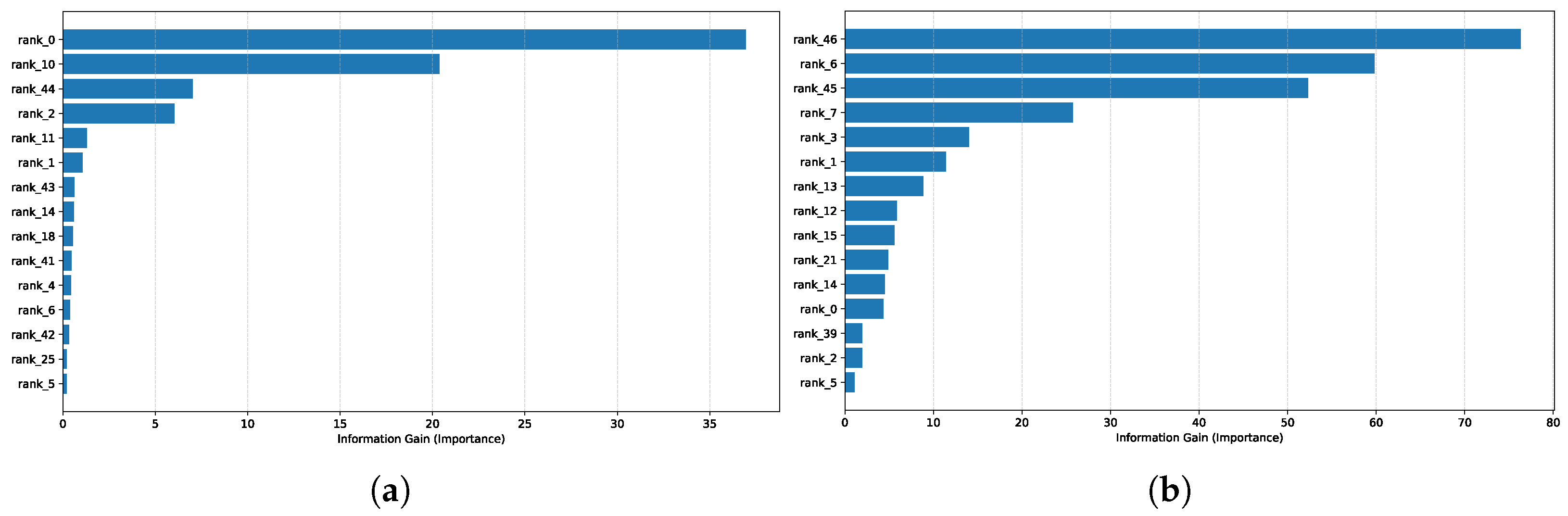
Analysis of the downstream classifier’s feature importance (Figure 6) points to the mechanism behind the Neural CDE’s stronger performance on the sparse CERT 6.2 dataset, and is consistent with the loss behaviour in Figure 5.

The discrete LSTM produces a high-variance error signal dominated by isolated spikes. As a result, the downstream classifier leans heavily on the single largest error (rank_0; Figure 6a)—a feature that is easily confused with ordinary day-to-day noise on this dataset, and which yields weak detection (F1 0.13).

The continuous NCDE instead produces a sharp but sustained elevation during anomalous windows (Figure 5(bottom)). This stability lets the classifier draw on lower-ranked, more robust features (e.g., rank_46; Figure 6b) rather than a single fragile outlier. The shift in which features carry importance—from an extreme-value feature for the LSTM to mid-rank features for the NCDE—is consistent with the NCDE’s continuity acting as a temporal smoother, and accompanies its substantially higher detection performance on 6.2 (F1 0.364 vs. 0.133; PR-AUC 0.288 vs. 0.034).

5. Conclusions

We presented a comparative study of LSTM and NCDE models for user anomaly detection across two CERT datasets. The continuous-time NCDE’s advantage proved to be regime-dependent: on the denser, less imbalanced CERT 4.2, the two models were competitive, whereas on the sparse, severely imbalanced CERT 6.2, the NCDE clearly outperformed the discrete LSTM baseline (F1 0.364 vs. 0.133; PR-AUC 0.288 vs. 0.034), surfacing four of the five malicious users with a sharp, localised error signal. This gain comes at the cost of substantially higher compute: per-user scoring took on the order of hours rather than minutes. For real-time use, this overhead is a genuine limitation, but for a daily batch screening job, it is likely acceptable—in high-stakes security settings, the cost of a missed insider far outweighs the additional training and inference cost of a more expensive model. The fact that the NCDE’s benefit is concentrated precisely in the sparse, imbalanced regime—the setting most representative of real insider-threat data—is what makes the added cost worthwhile.

While our empirical results demonstrate the practical utility of NCDEs for user anomaly detection, future work must establish a stronger theoretical foundation for this specific application. Real-world cybersecurity environments represent a highly complex reality, and while empirical experimentation yields actionable results, the mathematical guarantees of these continuous models require further scrutiny. Specifically, subsequent research should formally investigate the asymptotic stability, consistency, and convergence properties of the adaptive step-size solvers when subjected to the extreme sparsity and burstiness of UBA data. Furthermore, as the domain of Neural Differential Equations rapidly expands, future studies should build upon the foundational literature to explore newer continuous-time architectures that balance empirical performance with rigorous theoretical discretization limits.

References

- Glasser, J.; Lindauer, B. Bridging the Gap: A Pragmatic Approach to Generating Insider Threat Data. In Proceedings of the 2013 IEEE Security and Privacy Workshops, San Francisco, CA, USA, 23–24 May 2013; pp. 98–104. [Google Scholar] [CrossRef]
- Jurišić, M.; Tomičić, I.; Grd, P. User behavior analysis for detecting compromised user Accounts: A review paper. Cybern. Inf. Technol. 2023, 23, 102–113. [Google Scholar] [CrossRef]
- Rashid, T.; Agrafiotis, I.; Nurse, J.R. A new take on detecting insider threats: Exploring the use of hidden markov models. In Proceedings of the 8th ACM CCS International Workshop on Managing Insider Security Threats, Vienna, Austria, 28 October 2016; pp. 47–56. [Google Scholar]
- Le, D.; Zincir-Heywood, N.; Heywood, M. Analyzing Data Granularity Levels for Insider Threat Detection Using Machine Learning. IEEE Trans. Netw. Serv. Manag. 2020, 17, 30–44. [Google Scholar] [CrossRef]
- Al-Shehari, T.; Alsowail, R. Random resampling algorithms for addressing the imbalanced dataset classes in insider threat detection. Int. J. Inf. Secur. 2023, 22, 611–629. [Google Scholar] [CrossRef]
- Al-Shehari, T.; Al-Razgan, M.; Alfakih, T.; Alsowail, R.; Pandiaraj, S. Insider Threat Detection Model Using Anomaly-Based Isolation Forest Algorithm. IEEE Access 2023, 11, 118170–118185. [Google Scholar] [CrossRef]
- Peccatiello, R.; Gondim, J.; Garcia, L. Applying One-Class Algorithms for Data Stream-Based Insider Threat Detection. IEEE Access 2023, 11, 70560–70573. [Google Scholar] [CrossRef]
- Manoharan, P.; Yin, J.; Wang, H.; Zhang, Y.; Ye, W. Insider threat detection using supervised machine learning algorithms. Telecommun. Syst. 2024, 87, 899–915. [Google Scholar] [CrossRef]
- Bertrand, S.; Desharnais, J.; Tawbi, N. Unsupervised user-based insider threat detection using bayesian gaussian mixture models. In Proceedings of the 2023 20th Annual International Conference on Privacy, Security and Trust (PST); IEEE: Piscataway, NJ, USA, 2023; pp. 1–10. [Google Scholar]
- Tuor, A.; Kaplan, S.; Hutchinson, B.; Nichols, N.; Robinson, S. Deep learning for unsupervised insider threat detection in structured cybersecurity data streams. In Proceedings of the AAAI Workshop-Technical Report, San Francisco, CA, USA, 4–9 February 2017; Volume WS-17-01–WS-17-15, pp. 224–234. [Google Scholar]
- Paul, S.; Mishra, S. LAC: LSTM AUTOENCODER with community for insider threat detection. In Proceedings of the ACM International Conference Proceeding Series, Houston, TX, USA, 3–7 February 2020; pp. 71–77. [Google Scholar] [CrossRef]
- Yuan, F.; Shang, Y.; Liu, Y.; Cao, Y.; Tan, J. Data Augmentation for Insider Threat Detection with GAN. In Proceedings of the Proceedings-International Conference on Tools with Artificial Intelligence (ICTAI), Boca Raton, FL, USA, 9–11 November 2020; IEEE: New York, NY, USA, 2020; pp. 632–638. [Google Scholar] [CrossRef]
- Zhu, Y.; Li, H.; Liao, Y.; Wang, B.; Guan, Z.; Liu, H.; Cai, D. What to do next: Modeling user behaviors by time-LSTM. In Proceedings of the IJCAI, Melbourne, VIC, Australia, 19–25 August 2017; Volume 17, pp. 3602–3608. [Google Scholar]
- Kidger, P. On Neural Differential Equations. Ph.D. Thesis, University of Oxford, Oxford, UK, 2021. [Google Scholar]
- Ru, J.; Lu, B.; Chen, B.; Shi, J.; Chen, G.; Wang, M.; Pan, Z.; Lin, Y.; Gao, Z.; Zhou, J.; et al. Attention guided neural ODE network for breast tumor segmentation in medical images. Comput. Biol. Med. 2023, 159, 106884. [Google Scholar] [CrossRef] [PubMed]
- Moon, I.; Groha, S.; Gusev, A. SurvLatent ODE: A Neural ODE based time-to-event model with competing risks for longitudinal data improves cancer-associated Venous Thromboembolism (VTE) prediction. In Proceedings of the Machine Learning for Healthcare Conference; PMLR: New York, NY, USA, 2022; pp. 800–827. [Google Scholar]
- Jiao, L.; Song, X.; You, C.; Liu, X.; Li, L.; Chen, P.; Tang, X.; Feng, Z.; Liu, F.; Guo, Y.; et al. AI meets physics: A comprehensive survey. Artif. Intell. Rev. 2024, 57, 256. [Google Scholar] [CrossRef]
- Rehman, D.; Lienhard, J.H. Physics-informed deep learning for multi-species membrane separations. Chem. Eng. J. 2024, 485, 149806. [Google Scholar]
- Lindauer, B. Insider Threat Test Dataset; CERT Division: Pittsburgh, PA, USA, 2020. [Google Scholar] [CrossRef]
- Bartoszewski, F.; Just, M.; Lones, M.; Mandrychenko, O. Anomaly Detection for Insider Threats: An Objective Comparison of Machine Learning Models and Ensembles. IFIP Adv. Inf. Commun. Technol. 2021, 625, 367–381. [Google Scholar] [CrossRef]
- Song, S.; Gao, N.; Zhang, Y.; Ma, C. BRITD: Behavior rhythm insider threat detection with time awareness and user adaptation. Cybersecurity 2024, 7, 2. [Google Scholar] [CrossRef]
- Jurišić, M.; Tomičić, I. A Comparative Study of Continuous and Discrete Time Models for User Anomaly Detection, Version v1.0; Zenodo: Geneva, Switzerland, 2025. [Google Scholar] [CrossRef]
- Ansel, J.; Yang, E.; He, H.; Gimelshein, N.; Jain, A.; Voznesensky, M.; Bao, B.; Bell, P.; Berard, D.; Burovski, E.; et al. PyTorch 2: Faster Machine Learning Through Dynamic Python Bytecode Transformation and Graph Compilation. In Proceedings of the 29th ACM International Conference on Architectural Support for Programming Languages and Operating Systems, (ASPLOS ’24); ACM: New York, NY, USA, 2024; Volume 2. [Google Scholar] [CrossRef]
- Bradbury, J.; Frostig, R.; Hawkins, P.; Johnson, M.J.; Leary, C.; Maclaurin, D.; Necula, G.; Paszke, A.; VanderPlas, J.; Wanderman-Milne, S.; et al. JAX: Composable transformations of Python+NumPy Programs. 2018. Available online: https://github.com/jax-ml/jax (accessed on 24 June 2026). [PubMed]
- Chawla, N.V.; Bowyer, K.W.; Hall, L.O.; Kegelmeyer, W.P. SMOTE: Synthetic minority over-sampling technique. J. Artif. Intell. Res. 2002, 16, 321–357. [Google Scholar] [CrossRef]