Reconciling Negative Soil CO₂ Fluxes: Insights from a Large-Scale Experimental Hillslope

Abstract

Soil fluxes of CO₂ (F_s) have long been considered unidirectional, reflecting the predominant roles of metabolic activity by microbes and roots in ecosystem carbon cycling. Nonetheless, there is a growing body of evidence that non-biological processes in soils can outcompete biological ones, pivoting soils from a net source to sink of CO₂, as evident mainly in hot and cold deserts with alkaline soils. Widespread reporting of unidirectional fluxes may lead to misrepresentation of F_s in process-based models and lead to errors in estimates of local to global carbon balances. In this study, we investigate the variability and environmental controls of F_s in a large-scale, vegetation-free, and highly instrumented hillslope located within the Biosphere 2 facility, where the main carbon sink is driven by carbonate weathering. We found that the hillslope soils were persistent sinks of CO₂ comparable to natural desert shrublands, with an average rate of −0.15 ± 0.06 µmol CO₂ m² s⁻¹ and annual sink of −56.8 ± 22.7 g C m⁻² y⁻¹. Furthermore, higher uptake rates (more negative F_s) were observed at night, coinciding with strong soil–air temperature gradients and [CO₂] inversions in the soil profile, consistent with carbonate weathering. Our results confirm previous studies that reported negative values of F_s in hot and cold deserts around the globe and suggest that negative F_s are more common than previously assumed. This is particularly important as negative F_s may occur widely in arid and semiarid ecosystems, which play a dominant role in the interannual variability of the terrestrial carbon cycle. This study contributes to the growing recognition of the prevalence of negative F_s as an important yet, often overlooked component of ecosystem C cycling.

1. Introduction

Arid and semiarid ecosystems across the globe play a fundamental role in the interannual variability of the terrestrial carbon cycle [1,2] and might be considered model systems to understand a future world that is becoming drier and warmer [3]. Covering ~40% of the terrestrial surface [4] and increasing in area [5], arid and semiarid ecosystems traditionally have been considered to have low carbon uptake, mainly due to low vegetation productivity [6]. Nonetheless, for more than a decade evidence exists from plot to ecosystem scales (Supplementary Table S1) that non-biological processes might be important to the local C-cycle in arid and semiarid ecosystems [7,8,9], where the inorganic soil C pool can be up to 10 times greater than the organic C pool [10]. A number of studies have implicated strong and anomalous downward fluxes of CO₂ into soils as critical components of C cycling in these regions, which has received much attention [11,12,13].

Soil fluxes of CO₂ (F_s) drive significant carbon exchange between the terrestrial surface and the atmosphere, second only to photosynthesis [14,15]. Due to their temperature sensitivity, F_s are considered to be the main determinant of future feedbacks to ongoing global climate change and, on a global scale, contribute an order of magnitude more than does anthropogenic activity [16]. F_s have been historically considered a flux from soils to the atmosphere (i.e., positive soil CO₂ fluxes) driven by microbial decomposition of organic matter and respiration from roots and mycorrhizae [17]. However, a growing body of evidence shows that soils can also take up CO₂ (i.e., negative soil CO₂ fluxes), mainly in sparsely vegetated, cold or hot deserts, and with alkaline pH (Supplementary Table S1), although also seen in temperate forests [18]. The finding of bidirectional soil CO₂ fluxes suggests that other processes beyond metabolic/biological activity can dominate carbon cycling within the soil profile, both in space and time. However, the physical and biogeochemical mechanisms that promote capture of CO₂ by soils are still uncertain and spark debate, even regarding whether negative F_s represent carbon uptake by the ecosystem [19,20], especially over short temporal scales. This knowledge gap challenges confidence in the understanding and quantification of ecosystem carbon balance, from local to global scales.

A number of potential hypotheses have been proposed to explain anomalous carbon uptake across water-limited ecosystems, including the following: (i) nighttime uptake of CO₂ by crassulacean acid metabolism (CAM) photosynthesis [21]; (ii) growth of lichens, mosses and cyanobacteria [22]; and (iii) non-biological processes, such as weathering and leaching [23]. Rather than being exclusive, competition may occur within soils between biological and non-biological processes that determine the direction of F_s. A combination of above- and below-ground measurements of CO₂ and geochemical modeling determined that weathering reactions contribute considerably to the ecosystem carbon balance in shrubland with high levels of carbonaceous substrates [24]. Furthermore, carbonate reaction rates were found to be highly dynamic at short temporal scales, influencing the ecosystem net carbon balance, particularly during periods when the soil was dry. One of the principal characteristics of arid and semiarid ecosystems are seasonal dry spells, suggesting that this phenomenon should occur more frequently than expected (see Supplementary Table S1). Basalt weathering (i.e., from olivine: Mg₂SiO₄ + 2H₂CO₃ → 2Mg²⁺ + 2CO₃²⁻ + H₄SiO₄) and carbonate reactions (i.e., Ca²⁺ + 2HCO₃⁻ ⇆ CaCO₃ + CO₂ + H₂O), which are bidirectional at earth surface temperature and pressure, can draw CO₂ from the atmosphere into the soil and, eventually through runoff and discharge, lead to sedimentation into the oceans [25]. Weathering rates are influenced by changes in soil moisture, air-filled space [26], pH due to atmospheric deposition and drainage [24], temperature [27], reactive surface area [25], as well as [CO₂] and [cation; Ca²⁺, Mg²⁺] within the soil solution. The [CO₂] can be influenced by microbial and root respiration [17], whereas [cation] is most affected by reaction progress. Since there is ambiguity on the direction of carbonate weathering fluxes [24], we will consider carbonate dissolution (i.e., CaCO₃ + CO₂ + H₂O → Ca²⁺ + 2HCO₃⁻) as a sink since it represents a CO₂ uptake from the atmosphere into the soil, and carbonate precipitation (i.e., Ca²⁺ + 2HCO₃⁻ → CaCO₃ + CO₂ + H₂O) as a source of CO₂ emissions from the soil to the atmosphere [24]. Thus, if the strength of the carbonate dissolution (i.e., acting as a sink of CO₂) outpaces the strength of CO₂ sources (i.e., by microbial and root respiration, and carbonate precipitation), negative F_s could result.

A challenge to understanding the temporal variability of negative F_s is that most evidence and theory comes from laboratory experiments performed on disturbed soil samples that do not represent natural conditions and may overestimate weathering rates [26,28]. Moreover, most studies using flux chambers or soil probes for gradient fluxes that report negative F_s were based on short field campaigns (e.g., days to months; see studies in Supplementary Table S1). Commonly used automated techniques to measure F_s and net ecosystem exchange of C (e.g., eddy covariance technique) also have their limitations and pitfalls [29,30]. For example, the eddy covariance technique is limited under low turbulence conditions, estimates the net ecosystem exchange of CO₂ without information of its contributing components, and relies on flux partitioning algorithms that do not account for non-biological processes [31]. Furthermore, soil respiration chambers can introduce biases in estimations of F_s by disrupting stable atmospheric conditions during automated opening and closing [32]. Although the gradient method does not produce a similar disruption artefact, its main limitation comes from the sensitivity of F_s to the estimation of gas diffusion rates [33]. It is, therefore, a common practice to discard negative values of F_s because they are deemed improbable, although not impossible. Lastly, these kinds of automated measurements lack replication and potentially do not integrate spatial variability across the ecosystem [34,35,36].

Together, the expectation that F_s should only reflect biological respiration and the uncertainties inherent to measurement techniques may be limiting our understanding of the prevalence and variability of negative F_s. In this study, we use a large-scale research facility, the Landscape Evolution Observatory (LEO), consisting of artificial landscapes (surface area of 330 m²) filled with vegetation-free ground basaltic tephra and equipped with a dense array of sensors to monitor pore-space CO₂ concentrations and meteorological variables. Previous work in this system has shown that carbonate weathering is the principal process fixing carbon from the atmosphere into the LEO soil [26]. Here, we take advantage of this large-scale model system to explore the environmental drivers of F_s and the belowground dynamics that determine F_s. We hypothesized that (H1) negative F_s occurs only at night, as has been seen in previous studies in natural ecosystems using automated measurements (Supplementary Table S1) despite the study system being a large-scale hillslope with a controlled environment; and (H2) experimental hillslopes should demonstrate features similar to those in natural ecosystems where negative F_s are observed, such as subsurface temperature gradients and [CO₂] inversions [24,37]. Our overarching research goals were to describe the temporal patterns in F_s, as well as the frequency and strength of negative F_s at LEO, and to determine the extent to which physical processes drive negative F_s.

2. Materials and Methods

2.1. Study Site and Environmental Conditions

The Biosphere 2—Landscape Evolution Observatory (LEO) consists of three identically replicated experimental hillslopes (30 m × 11 m = 330 m² surface area, with 10° average slope and uniform 1-m depth). Soils at LEO are basalt with a loamy sand texture and a bulk density of 1.5 g cm⁻³. For more information about the LEO facilities see References [38,39,40]. Here, we used a year-long time series of data obtained between November 2016 and November 2017 from one of the LEO hillslopes (referred to as LEO East). During this period, three different conditions of environmental forcing prevailed. In the first condition (October to December 2016, R-I in Figure 1B), two successive irrigation pulses (each of 3-h duration and 36-mm magnitude) were applied every 3.5 days. In the second condition (April to August 2017, R-II in Figure 1B), one irrigation pulse (9-h duration and 108-mm magnitude) was applied every 14 days. Finally, in the third condition (August to October 2017, R-III in Figure 1B), one irrigation pulse was applied every 28 days. These three conditions were interspersed by several-week-long periods without irrigation. As such, this controlled experiment offered a variety of reproducible environmental conditions, ranging between extremely wet and dry.

2.2. Environmental Measurements

LEO hillslopes are systematically instrumented below and above ground. In each hillslope, gaseous CO₂ within the soil is measured with solid-state CO₂ sensors (GMM 220, Vaisala, Helsinki, Finland) at 48 locations at four different depths (5 cm, 20 cm, 35 cm, and 50 cm). Soil temperature and moisture sensors (5TM, Decagon, Pullman, WA, USA), and soil water potential sensors (MPS-2, Decagon, Pullman, WA, USA) are distributed across 496 sampling locations in each hillslope at five different depths (5 cm, 20 cm, 35 cm, 50 cm, and 85 cm). Air temperature and relative humidity are monitored in 25 locations at five different heights (0.25 m, 1 m, 3 m, 6 m, and 9 m) above the hillslope surface. Measurements of atmospheric CO₂ are made using an infrared gas analyzer (LI-7000, LICOR, Biosciences, Lincoln, NE, USA). We averaged the time series of environmental variables measured belowground in different locations by depth (i.e., 5 cm, 20 cm, 35 cm, 50 cm), and aboveground measurements were averaged across all sampling locations and heights. Data from LEO is publicly available (http://www.biosphere2.org/research/leo-data).

2.3. CO₂ Flux Estimation

F_s (µmol CO₂ m⁻² s⁻¹) was estimated based on Fick’s law of diffusion:

$$F_s=-D_s\frac{\partial C}{\partial Z}$$

(1)

where D_s is the diffusion coefficient (m² s⁻¹), C is the CO₂ molar density (µmol m⁻³), computed using the universal gas law, and Z is depth (m). To estimate D_s, we included the diffusion of gases within the soil matrix in the gas and liquid phases:

$$D_s=\left[D_w+D_a\right]$$

(2)

where D_w (m² s⁻¹) is the diffusion coefficient in the liquid phase, and D_a (m² s⁻¹) is the diffusion of gases in free air. Here, we estimated the D_w coefficient as [41]:

$$D_w=\frac{{\theta }^{10/3}{D}_{fw}}{H}{\varnothing }^{-2}$$

(3)

where θ is the soil volumetric water content (m³ m⁻³), D_fw is the diffusion coefficient of CO₂ in free water, H is the dimensionless form of Henry’s solubility constant for CO₂ in water (H = 0.8317), and ø is the total soil porosity. D_a is expressed as [42]:

$$D_a={\varnothing }^2{\left(\frac{\vartheta }{\varnothing }\right)}^{\beta S}$$

(4)

where β = 2.9, S = silt + sand percentage (84.6 + 12.2 = 96.8%), and ϑ represents the air-filled porosity (m³ m⁻³):

$$\vartheta =\varnothing -\theta$$

(5)

where ø is the total soil porosity:

$$\varnothing = 1-\frac{BD}{PS}$$

(6)

where BD is the soil bulk density (1.5 g cm⁻³), and PS is the soil particle density size (2.65 g cm⁻³). To account for the effects of temperature and pressure on D_a, we followed Reference [43]:

$$D_a=D_{a0}{\left(\frac{T}{T_0}\right)}^{1.75}\left(\frac{P_0}{P}\right)$$

(7)

where D_a0 is a reference value of D_a (1.47 × 10⁻⁵ m² s⁻¹) at a reference temperature (T₀ = 293.15 K) and reference pressure (P₀ = 1.013 × 10⁵ Pa). Our formulation of D_a has been used widely across different ecosystem types [44].

The diffusion coefficient D_s in soil was calculated separately for each soil layer. CO₂ was assumed to move between soil layers due to physical displacement, driven by water replacing air in the soil–pore space [45]. Thus, at each time step a new [CO₂] in each layer (ΔC), the product of CO₂ transport between layers, was calculated as a function of the layer depth [46]:

$$\Delta C=\frac{\left[{\vartheta }_z\left(t_i\right)-{\vartheta }_z\left(t_{i+1}\right)\right] l_z C_z\left(t_i\right)}{t_{i+1}-t_i},$$

(8)

where ϑ_z(t_i) is the air-filled porosity of depth Z at time t_i, l_z (m) is the thickness of each layer (i.e., 5 cm for the first layer and 15 cm the next three layers), and C_z(t_i) is the [CO₂] at depth Z at time t_i. Thus, the total F_s was estimated in individual soil layers (L) and calculated based on the mass balance of CO₂:

$$F_{s,L}=J_L-J_{L-1}+\Delta C+\left(C_Z\left(t_{i+1}\right)-C_Z\left(t_i\right)\right) {\vartheta }_z,$$

(9)

where J_L is the CO₂ transport from soil layer L to L + 1 (i.e., from 20 cm to 5 cm), J_L−1 is the CO₂ transport from soil layer L − 1 to L (i.e., from 35 cm to 20 cm), and C_Z is the [CO₂] of depth Z at time t_i. Note that we consider the thickness of the layer from one sensor to another in depth (i.e., layer thickness of 15 cm between sensors at 5 and 20 cm). For a graphical representation of Equation (9) the reader is referred to Supplementary Figure S1.

Previously, Cueva et al. [47] estimated the uncertainties for two different algorithms to calculate the soil CO₂ efflux across different ecosystems, including semiarid, and found that the uncertainty due to random errors is relatively small (i.e., from 0.38 to 2.39% of the annual sum). Here, following References [48] and [49], we estimated the uncertainty of F_s, by summing the squares of the components errors and then taking the square root, yielding an uncertainty of ±0.22% of our annual sum.

Note that we used the same sign convention to report CO₂ fluxes as in eddy covariance literature [50], where a net addition of CO₂ to the atmosphere is a positive flux, and a net loss of CO₂ from the atmosphere is a negative flux unless otherwise noted. For example, we consider carbonate dissolution as a sink since it represents a CO₂ uptake from the atmosphere into the soil, and carbonate precipitation as a source since it causes a CO₂ emission from the soil to the atmosphere [24].

2.4. Statistical Analysis

To establish relationships with environmental data, we bin-averaged hourly estimated F_s according to the environmental variable in equally spaced bins of one unit (i.e., each 1 m s⁻¹ × 10⁻⁶ for soil diffusion, each 1 kPa for water potential), unless otherwise noted.

To estimate the activation energy of F_s, we used the Arrhenius equation [51]:

$$F_s=A^{\left(-Ea/RT\right)},$$

(10)

where Ea is the activation energy (kJ mol⁻¹) of the reaction, T is the temperature (K), R is the gas constant (R = 8.31 × 10⁻³ kJ K⁻¹ mol⁻¹), and A is the pre-exponential constant. The temperature sensitivity of F_s was estimated using a Q₁₀ function [52]:

$$F_s=F_{10} Q_{10}{ }^{\left(\left(T-10\right)/10\right)},$$

(11)

where F₁₀ is the simulated flux at 10 °C, Q₁₀ is the temperature sensitivity of F_s, and T (°C) is soil temperature. Both Ea and Q₁₀ were estimated using daily averages of F_s and soil temperature at 5 cm. Estimations of F_s and all statistical analyses were performed in Matlab (R2017a, Mathworks).

3. Results

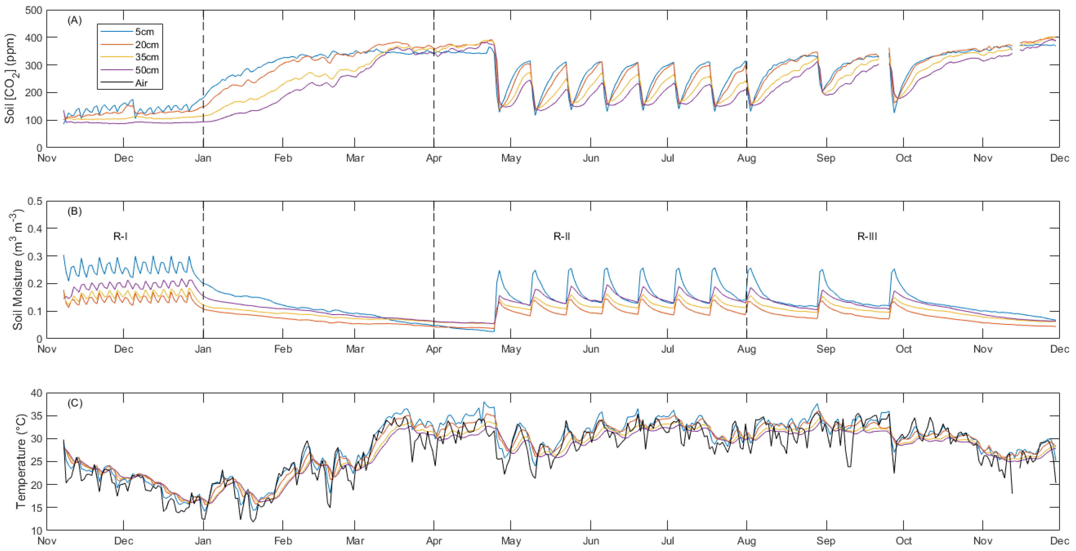
3.1. General Environmental Conditions at LEO

Air temperature (averaged across the whole study period) was slightly lower than the average soil temperature at the shallowest measurement depth, and average soil temperature decreased with depth (

Table 1. Average ± standard deviation of environmental conditions above and belowground in the Landscape Evolution Observatory.

	Temperature (°C)	Moisture (m3 m−3)	[CO2] (ppm)
Air	27.13 ± 10.51	--	387.16 ± 28.13
Soil
5 cm	28.56 ± 6.90	0.15 ± 0.07	273.50 ± 81.08
20 cm	28.32 ± 5.42	0.09 ± 0.03	268.54 ± 88.66
35 cm	27.52 ± 5.05	0.11 ± 0.03	240.17 ± 88.54
50 cm	27.14 ± 4.80	0.13 ± 0.04	218.19 ± 90.01

). Both air and soil temperature displayed a seasonal cycle and were lowest during wintertime and highest in the summertime (Figure 1). Atmospheric CO₂ concentrations ([CO₂]) within the LEO domain were similar to local ambient concentrations (~400 ppm). However, soil [CO₂] were lower than in the LEO atmosphere and decreased with depth (Table 1, Figure 1). Soil moisture within the soil profile was on average highest at the top measurement depth and lowest at the second measurement depth (Table 1, Figure 1). Furthermore, soil moisture and [CO₂] followed consistent and reproducible wet–dry patterns in response to the rainfall manipulation experiments (Figure 1).

Soil CO₂ fluxes (F_s) estimated by the gradient method showed persistently negative values across the study period (Figure 2), representing an influx of CO₂ from the atmosphere into the soil, with an average (± standard deviation) F_s of −0.15 ± 0.06 µmol CO₂ m² s⁻¹, and annual F_s of −57 ± 23 g C m⁻² y⁻¹. Moreover, F_s also showed wetting–drying patterns corresponding to the rainfall manipulation experiments. The lowest value of F_s (i.e., most negative or highest uptake flux) was observed after a prolonged drying period at the end of April (i.e., before the start of the second rainfall condition), and F_s became less negative (i.e., closer to zero) immediately following each rain event.

3.2. Diurnal Variability

We found different diurnal patterns in soil [CO₂] in relation to soil depth. On the diurnal scale, soil [CO₂] dynamics showed a temporal lag between the 5 and 20 cm measurement depths: [CO₂] peaked first at 5 cm, were highest during daytime at 5 cm, and were highest during nighttime at 20 cm (Figure 3). Soil [CO₂] at 35 and 50 cm depth also varied diurnally, however, with lower amplitude than at 5 and 20 cm depth (Figure 3). Furthermore, soil [CO₂] at 35 and 50 cm were much lower than in the upper layers (e.g., consistently lower [CO₂]). Nor did the [CO₂] at 35 and 50 cm overlap as found in the shallower layers.

Soil temperature also showed distinct temporal lags among layers in comparison to air temperature (Figure 3). Air temperature peaked earliest in the day, followed by a peak of soil temperature at 5 cm, while soil temperature at 20 cm was lowest around midday and increased during the afternoon–nighttime hours (Figure 3). In addition, like [CO₂] with depth, the amplitude of the diurnal variation in temperature decreased with depth. We also noted a slight temporal lag between soil [CO₂] and temperature at 5 cm, with [CO₂] peaking first. F_s in each layer varied diurnally, although without an evident temporal lag, switching in positive to negative values at 20 and 35 cm depth (Figure 3). F_s in the top layer (0–5 cm) became less negative during daytime and was most negative at night (Figure 3). F_s at the second layer (5–20 cm) was negative during the daytime (after midday) and switched to positive values during the afternoon and remained positive most of the night (Figure 3). F_s in the bottom layers (20–35 cm and 35–50 cm) were close to zero and showed weak diurnal variability in the third layer (20–35 cm) with nearly constant values in the lowermost layer (35–50 cm; Figure 3).

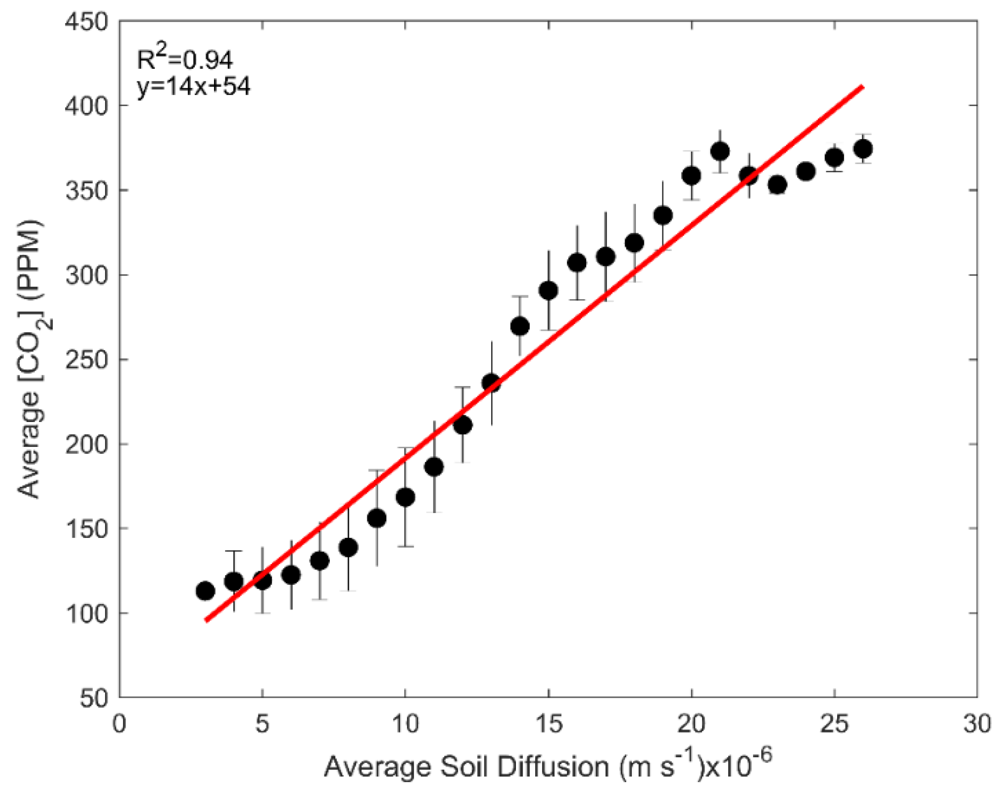
3.3. Physical Drivers of Negative Soil CO₂ Fluxes

We found a positive linear relationship (p < 0.05, R² = 0.94) between the profile-average soil [CO₂] and profile-average soil diffusion coefficient (D_s; Figure 4). This relationship indicates that as soil diffusivity increases, [CO₂] (sourced from the atmosphere) within the soil profile also increases. However, contrary to the case of soil [CO₂], when we compared F_s with D_s we did not find a linear relationship (Figure 5). Instead, F_s demonstrated the following three phases in relation to D_s: (1) Low soil diffusion coefficients (D_s) between 0 and ~7 × 10⁻⁶ m s⁻¹, when soil water content (SWC) was greater than 0.2 m³ m⁻³, and F_s became more negative (higher uptake rates) as D_s increased; (2) a pivot of F_s increasing towards less negative values (lower uptake rates), while D_s values increased between ~7 and ~15 × 10⁻⁶ m s⁻¹ and SWC decreased between 0.1 and 0.2 m³ m⁻³; and (3) a return to the trend of F_s becoming more negative (higher uptake rates) while D_s increased to values greater than 15 × 10⁻⁶ m s⁻¹ and SWC decreased to less than 0.1 m³ m⁻³.

A similar relationship was observed between F_s and soil water potential (ψ), which had the following two main phases (Figure 6): (1) at high soil water potential (ψ between −5 kPa and −20 kPa) values of F_s become less negative (uptake rates decrease) from approximately −0.18 to −0.9 µmol CO₂ m² s⁻¹; and (2) at lower soil water potential values (ψ < −20 kPa) F_s becomes more negative (uptake rates increase) from approximately −0.9 to −0.25 µmol CO₂ m⁻² s⁻¹.

We found a significant relationship (p < 0.05, R² = 0.92, Figure 7) between surface F_s and the temperature difference between air and soil (T_air − T_soil). Thus, F_s was more negative (stronger uptake) when T_soil > T_air, and as the temperature gradient increases changed to T_air > T_soil, F_s became less negative. We also found a clockwise hysteresis relationship between F_s and surface T_soil across the diurnal cycle (Figure 8). This hysteresis showed the lowest values (strongest uptake) of F_s during nighttime, moving to values of F_s closer to zero (less uptake) during daytime (Figure 8). Additionally, we found that the activation energy (Ea; Equation (10)) of the relationship of F_s with soil temperature at 5 cm was significant (p < 0.001) with a value of 74.02 kJ mol⁻¹, although only a small proportion of the variability was explained (R² = 0.19) (Figure 9). The overall temperature sensitivity of F_s in this LEO hillslope was Q₁₀ = 1.31 ± 0.07 (dimensionless).

4. Discussion

The LEO hillslope basalt soils constantly removed CO₂ from the atmosphere and at rates similar to previous studies that used automatic measurements of F_s in natural ecosystems, including hot and cold deserts [37,53,54,55]. On an annual basis, LEO soils functioned as a net C sink (F_s = −56.8 ± 22.7 g C m⁻² y⁻¹) with a magnitude comparable to the net ecosystem exchange of CO₂ in a desert shrub community (−52 g C m⁻² y⁻¹; [21]), a mature semiarid shrubland (−52 g C m⁻² y⁻¹; [56]), both using the eddy covariance technique, and a saline desert (−62 g C m⁻² y⁻¹; [57]) using respiration chambers. However, we have to highlight that LEO had a higher water availability than those natural ecosystems. Moreover, we found more negative F_s (more uptake) at night (partially supporting our H1), coinciding with strong soil–air temperature gradients, and [CO₂] inversions in the soil profile (supporting H2). These results corroborate previous evidence of negative F_s in natural ecosystems (Supplementary Table S1) and suggest that negative F_s are a more prevalent phenomenon than previously assumed. Here we discuss the implications of these results.

4.1. Reversible Flux or Sequestration

There is a growing debate about whether negative F_s observed across natural ecosystems represent a true uptake of CO₂ from the atmosphere into soils [19,20,58]. There are various non-biological mechanisms that could explain such anomalous CO₂ uptake, including pressure pumping and atmospheric turbulence [23]. F_s estimates, combined with soil solution and seepage export, C chemistry across several rainfall events, could be used to close the carbon balance of an LEO hillslope [26], confirming the sequestration potential of a basalt hillslope landscape. However, as stated by References [19] and [26], this uptake inferred from flux measurements was one-to-two orders of magnitude lower (i.e., less CO₂ uptake from the atmosphere to the soil) than laboratory estimates of carbonate weathering rates. Moreover, Reference [24] found that carbonate weathering fluxes can be highly dynamic. Since weathering reactions are bidirectional (i.e., carbonate dissolution and precipitation), they should have a relatively small effect on global carbon uptake on month to annual time-scales because of constant changes in disequilibrium due to fluctuations in: (1) CO₂ concentration within the soil profile; (2) moisture; and (3) atmospheric conditions. Although these fluxes are significant, carbonate weathering may not represent a missing carbon sink, as previously thought [8,13], but is nonetheless often overlooked.

A common practice is to discard fluxes close to or below zero when using respiration chambers or the gradient method. This is partially due to quality assurance and control (QA/QC) procedures based on the R² parameter of a linear relationship between time and [CO₂] inside the chambers [34]. Moreover, a pervasive rule of thumb has been to assume that F_s is only positive (i.e., fluxes from the soil to the atmosphere). However, increasing evidence indicates that negative F_s are potentially common and feasible (see Supplementary Table S1), and not an artefact of the measurement methods. Furthermore, negative F_s are commonly present at nighttime, while soil CO₂ fluxes—measured with manual and portable equipment during short field campaigns—are mainly gathered during daytime [59]. Negative F_s are likely most prevalent in ecosystems with high levels of carbonates, which includes ~10% of the terrestrial surface [23], low-density vegetation cover [53,60], and in systems with high pore connectivity [24]. Furthermore, we found that negative F_s have mostly been seen in alkaline soils, with pH values of 8.7 ± 1.1 (average ± standard deviation of data from Supplementary Table S1), in line with the global pH values of soil carbonate distribution [61].

4.2. Temporal Variability

We found that F_s followed a diurnal pattern and that the sign and magnitude depended on soil depth (Figure 3). Negative F_s in the soil surface reached lowest values at night [37,62,63]. We did not observe positive F_s (i.e., CO₂ moving from the soil to the atmosphere). This could have two potential explanations: (1) Weathering reactions within the LEO slopes generate an inverted [CO₂] gradient, i.e., [CO₂] is higher in the atmosphere than in the soil (Figure 3), thus, preventing an efflux; (2) lack of vegetation and the highly oligotrophic nature of the LEO soils, with incipient amounts of organic matter (7.03 ± 1.63 × 10⁻⁵ g C g dry soil⁻¹; [38]), limit the potential of CO₂ production within the slopes through respiration/metabolic activity. However, we did find that F_s became less negative (i.e., closer to zero) throughout the day. Microbial life does exist in LEO soils [39,40], and as a result, metabolic processes are present and could be more active during the daytime, mainly due to the relationship between temperature and microbial respiration [16,51,64]. Nonetheless, CO₂ production by microbes in LEO soils was apparently not enough to switch from negative to positive F_s. Furthermore, we cannot discard that heterotrophic bacterial carbonatogenesis or microbial induced carbonate precipitation [65,66,67], or the fixation of carbon from the atmosphere by autotrophic microorganisms [68] could drive a carbon sink, removing CO₂ from the atmosphere into the soil.

The diurnal variability of F_s changes in magnitude and sign as a function of soil depth, with greater amplitudes in the first two layers of soil (i.e., 0–5 cm and 5–20 cm). We noted that F_s values were more negative at night in the 0 to 5 cm layer. However, the F_s from the 5 to 20 cm layer to the 0 to 5 cm layer were positive (Figure 3C). Positive F_s from the 5 to 20 cm layer coincided with a temperature (Figure 3B) and soil [CO₂] inversion (Figure 3A). This suggests that CO₂ consumption uptake occurs in the soil surface layer of LEO, with CO₂ supplied both from atmospheric and from deeper layers of the soil, in agreement with References [24,37]. Carbonate saturation state changes can induce a diurnal cycle, where carbonate formation/precipitation and atmospheric ventilation/turbulence have been suggested to drive this pattern [24], mainly driven by the supply and removal of CO₂ through transport and carbonate dissolution and precipitation reactions. In this case, low daytime soil [CO₂] are due to ventilation/turbulence that induce a sustained CO₂ geochemical production due to carbonate precipitation (i.e., Ca²⁺ + 2HCO₃⁻ → CaCO₃ + CO₂ + H₂O). At night, ventilation/turbulence decreases and coupled with the inverted [CO₂] gradient at LEO, CO₂ migrates from deeper layers due to advection to shallower layers (Figure 3), where carbonate dissolution occurs (i.e., CaCO₃ + CO₂ + H₂O → Ca²⁺ + 2HCO₃⁻), resulting in a CO₂ consumption.

Other studies have suggested that outgassing of CO₂ from deeper layers, mainly due to cracks and caves, could be the cause of this weathering at shallower soil layers, especially during the day [23,24,53]. However, LEO hillslopes are relatively shallow in depth (1 m), and physically isolated by its steel structure, and carbonate was always chemically undersaturated at all depths [69]. Thus, this change in sign of F_s in the shallower layers could be a result of convective exchange, mainly due to the inversion of air and soil temperature across the profile [37,70]. This was supported by the relationship between F_s and the difference in air and soil temperature (Figure 7), where strong temperature gradients were associated with more negative F_s.

4.3. Physical vs. Biological Drivers

Soil diffusion (D_s) strongly controlled F_s, and low D_s limited CO₂ movement within the soil profile (Figure 1 and Figure 4), especially during the first days after the rain events. Since CO₂ is a precursor to carbonic acid, the main reactant in carbonate weathering, weathering rates were consequently limited [26]. The limitation of CO₂ movement resulted in F_s values closer to zero, though never pivoting towards positive values. Other studies have found that during wet periods negative F_s were not observed [37], however, in more saline and sandy environments negative F_s were observed and remained constant or even became more negative during the rainy period [53,71]. This effect (e.g., pivoting between negative and positive F_s) might be a result of enhanced respiration activity by roots and microorganisms tied to the vegetation cover in those natural ecosystems. In environments with vegetation cover, such as the Chihuahuan desert where the vegetation cover was 34% [37], positive F_s indicated that microbial metabolism and root respiration could dominate the total F_s, especially during wet periods [72]. While in saline and sandy environments [53,71], where vegetation cover was less than 20%, CO₂ uptake outpaced biological respiration, and the net F_s remained negative. Thus, in non-vegetated LEO hillslopes it is more likely that non-biological processes dominate, and although microbes are present, their metabolic contribution is not yet significant enough to shift the sign of F_s.

The correlation between F_s and D_s may give insights into microbial activity in the LEO soils (Figure 5). If this simple system was only driven by diffusion, we would expect this relationship to be linear or to follow a decay function. However, we found that for intermediate SWC conditions, there is an absolute increase of F_s towards zero. This could be explained at high moisture levels by low diffusion rates in saturated soil, leading to [CO₂] and [O₂] depletion within the soil, limiting both weathering and microbial activity. On the other hand, when the soil is very dry, despite the availability of [CO₂], microbial metabolism is limited by water availability. The relationship of F_s and water potential (ψ) at ψ <−20 kPa appears to point to a microbial respiration limitation (Figure 6). ψ plays a fundamental role in microbial metabolism and activity [73,74,75,76], and our results agree with the meta-analysis of [77]. Cessation of microbial respiration generally occurs at ψ less than−15 MPa in mineral soils [74]. In LEO, we measured a lower threshold of cessation (approx. −20 kPa ψ or −0.02 MPa), which corresponds to the limit for the cessation of bacterial motion [75]. Thus, our results can be seen as a lower potential threshold for the response of microbial metabolism to ψ in highly oligotrophic soils. In contrast with laboratory and field studies, where the optimal value of ψ for microbial respiration is close to field capacity (approx. −33 kPa) [78], our observed higher (i.e., less negative) potential threshold of ψ for the cessation of microbial activity could be due to the low amount of nutrients or water retention characteristics in the LEO hillslopes.

4.4. Temperature Relationship and Hysteresis

We found that the activation energy (Ea), inferred from the inverse of the soil temperature and the natural logarithm of F_s (Figure 9), of LEO soils (74.02 kJ mol⁻¹) is similar to other studies where Ea of weathering reactions was estimated in laboratory experiments. For example, the Ea of silicate weathering reactions in the Yamuna River system across the Himalaya varied between 51 and 83 kJ mol⁻¹ for sodium and silicon [79]; however, our Ea value is almost double those reported in a global synthesis of basalt weathering (i.e., ~37 to ~42 kJ mol⁻¹) [80]. We have to note that Ea could vary across different thresholds of soil moisture, as has been previously seen in the field [81,82] and in synthetic [83] experiments. This implies that weathering reactions in natural conditions also varies across seasons influenced by water availability, a common feature of arid and semiarid ecosystems, although it remains for further testing. A higher Ea of negative F_s for carbonate weathering indicates a less reactive and more recalcitrant substrate and should have a higher temperature sensitivity. Thus, despite basalt areas only representing a small fraction of the terrestrial surface (~3.5 to 5%) [80], the increasing trends in temperature across the globe could create a feedback in the terrestrial carbonate system, increasing weathering rates. Nonetheless, caution must be taken since carbonate weathering is a bidirectional reaction, but a stable and recalcitrant carbon sink.

Our estimated temperature sensitivity (Q₁₀ = 1.31 ± 0.07) is in line with previous findings [84,85]. Our results imply that an increase in temperature could also increase the carbonate weathering rates. However, caution has to be taken in the interpretation of our findings. Our F_s estimates have to be taken as a net flux (i.e., a combination of abiotic and biotic processes). Thus, our Q₁₀ estimate is a composite of different temperatures sensitivities (e.g., carbonate weathering, microbial metabolism, and growth). As discussed by Reference [34] for aboveground carbon fluxes, those processes may have different feedback mechanisms. For example, the increase in [CO₂] in the atmosphere could positively feedback carbonate dissolution (i.e., CaCO₃ + CO₂ + H₂O → Ca²⁺ + 2HCO₃⁻). Moreover, in the last decades, soil microbial respiration has been increasing providing additional CO₂ [86]. These sources of CO₂ could increase carbonate weathering rates. Our Q₁₀ estimates could vary across different soil moisture conditions, as has been noted previously for positive F_s [87,88]. This indicates that the temperature sensitivity of weathering rates can fluctuate seasonally. As suggested by Reference [89], there is a need to better comprehend the interactions and feedbacks between increases in [CO₂] and temperature on carbonate weathering rates.

We found a clockwise diel hysteresis in the relationship between F_s and soil temperature (Ts) (Figure 8). Diel cycles have been seen across natural ecosystems with positive [90,91,92], and negative [37,71] F_s, as well as in simulation models [93]. It is noteworthy that in studies reporting negative F_s, the hysteresis direction is clockwise, indicating that F_s peaked before Ts, while in sites that do not report negative F_s the hysteresis direction is counterclockwise, indicating that Ts peaked first. There is a consensus that these hysteresis loops could result from different biophysical factors, including photosynthetic carbon supply [90,94,95], non-rainfall water inputs, such as hydraulic redistribution by roots [96], and lateral transport of mist/fog/marine breeze [97], different temperature sensitivity of biological (e.g., microbial and root respiration) and non-biological (e.g., carbonate weathering) activity [34], temporal lags between CO₂ production/consumption and the actual surface CO₂ flux [95], unrepresentative measurement depths of temperature in relation to CO₂ production/consumption [52], and thermal diffusivity [93]. In the LEO hillslopes, we can discard plant photosynthetic carbon supply and root-associated autotrophic respiration, as well as non-rainfall water inputs, but there could be confounding effects for different temperature sensitivities for microbial metabolism and carbonate weathering. Soper et al. [98] found in the Mojave Desert that carbonate precipitation (i.e., positive F_s) occurs at high soil surface temperatures (e.g., >33–75 °C), and there is evidence that the biological component of F_s decreases substantially between 20 °C and 50 °C across hot deserts [99]. Thus, a combination of different processes producing and consuming CO₂ within the soil can influence the temperature relationship with F_s. Moreover, during nighttime when soils are cooling, there could be a migration of air from deeper soil to upper soil horizons, as seen in this study (Figure 3) and Reference [37], promoting carbonate dissolution (e.g., negative F_s). Thus, this combination of biological and non-biological components could result in different temperature sensitivities, which might be expected to vary across landscapes. Currently, flux partitioning algorithms for eddy covariance data do not take into account the non-biological component of ecosystem C fluxes [31], which may lead to biases in estimated ecosystem respiration and gross primary productivity in some ecosystems.

5. Conclusions

Here we demonstrated that LEO hillslopes are a consistent carbon sink, with comparable CO₂ flux rates to natural deserts across the globe. We showed that negative soil CO₂ fluxes are possible and probable, and should not be discarded in future studies, as they can influence local carbon balances that, in turn, propagate into global estimates. Our results from this large-scale experimental hillslope agreed with previous studies on the biophysical controls of negative soil CO₂ fluxes in natural ecosystems, giving insights into key controlling environmental factors. Negative soil CO₂ fluxes could be more prevalent across arid and semiarid ecosystems representing ~40% of the terrestrial surface. Mainly driven by non-biological processes, in alkaline soils with high levels of carbonate and low vegetation cover, these negative fluxes should be further studied to better comprehend their potential as a carbon sink. If the strength of the CO₂ sink due to non-biological processes (i.e., basalt and carbonate weathering) results to be considerable under short periods, further experimentations should be done to address current uncertainties, especially due to soil management [58].

Soil CO₂ fluxes are bidirectional and can shift in sign in response to the predominance of various biological and non-biological components. This work implies measured (e.g., with respiration chambers) and estimated (e.g., with the soil gradient method) soil CO₂ fluxes actually reflect a net soil exchange (NSE), analogous to the net ecosystem exchange (NEE), rather than only respiration or efflux [100]. In most ecosystems across the globe, NEE is usually negative, representing a fixation of CO₂ from the atmosphere through photosynthetic fixation into the biosphere, but exceptions in time and space have been reported [101]. Similarly, the NSE is commonly positive across the globe, where metabolic and respiratory processes dominate, representing, from the perspective of soils, a loss of CO₂ from the soil to the atmosphere. While these processes dominate, there are again exceptions in time and space, including the fixation of CO₂ in soils as a result of non-biological processes as we observed in the LEO system.

The concept of NSE requires new source partitioning methods for quantifying various biological and non-biological components, analogously to eddy covariance flux partitioning algorithms used to estimate the gross primary productivity and ecosystem respiration [102,103]. These may include isotopic methods to distinguish different CO₂ sources, such as been done in the Mojave Desert to differentiate biological from non-biological CO₂ production in the soil, due to the different δ¹³C signatures between the soil organic carbon and carbonates [98,104]. Additional measurements should be considered to interpret biological CO₂ production within the soil profile. The apparent respiratory quotient (i.e., ratio of CO₂ efflux to the oxygen influx) was used to show that the biological respiration rate was 3.8 times higher than the surface-measured CO₂ with chambers [105]. Furthermore, incorporating oxygen measurements within the soil profile will improve the capability of current state-of-the-art microbial enzyme models [81,106].

Finally, we believe that the concept of the NSE could be broadly used across different soil biogeochemical cycles. For example, methane (CH₄) can be both produced (i.e., methanogenesis) or consumed (i.e., methanotrophy) within the soil [107]; similarly, carbonyl sulfide (COS/OCS) fluxes are thought to be a combination of biological and non-biological sources [108,109]. Such features of soil gases can be used to develop soil functional types [110], analogous to plant and ecosystem functional types, to better represent soil functionality at global scales.

References

1. Ahlström, A.; Raupach, M.R.; Schurgers, G.; Smith, B.; Arneth, A.; Jung, M.; Reichstein, M.; Canadell, J.G.; Friedlingstein, P.; Jain, A.K.; et al. Carbon cycle. The dominant role of semi-arid ecosystems in the trend and variability of the land CO2 sink. Science 2015, 348, 895–899. [Google Scholar] [CrossRef] [PubMed]
2. Poulter, B.; Frank, D.; Ciais, P.; Myneni, R.B.; Andela, N.; Bi, J.; Broquet, G.; Canadell, J.G.; Chevallier, F.; Liu, Y.Y.; et al. Contribution of semi-arid ecosystems to interannual variability of the global carbon cycle. Nature 2014, 509, 600–603. [Google Scholar] [CrossRef]
3. Baldocchi, D.; Chu, H.; Reichstein, M. Inter-annual variability of net and gross ecosystem carbon fluxes: A review. Agric. For. Meteorol. 2018, 249, 520–533. [Google Scholar] [CrossRef]
4. Reynolds, J.F.; Smith, D.M.S.; Lambin, E.F.; Turner, B.L.; Mortimore, M.; Batterbury, S.P.J.; Downing, T.E.; Dowlatabadi, H.; Fernández, R.J.; Herrick, J.E.; et al. Global desertification: Building a science for dryland development. Science 2007, 316, 847–851. [Google Scholar] [CrossRef]
5. Andela, N.; Liu, Y.Y.; van Dijk, A.I.J.M.; de Jeu, R.A.M.; McVicar, T.R. Global changes in dryland vegetation dynamics (1988–2008) assessed by satellite remote sensing: Comparing a new passive microwave vegetation density record with reflective greenness data. Biogeosciences 2013, 10, 6657–6676. [Google Scholar] [CrossRef]
6. Noy-Meir, I. Desert Ecosystems: Environment and Producers. Annu. Rev. Ecol. Syst. 1973, 4, 25–51. [Google Scholar] [CrossRef]
7. Emmerich, W.E. Carbon dioxide fluxes in a semiarid environment with high carbonate soils. Agric. For. Meteorol. 2003, 116, 91–102. [Google Scholar] [CrossRef]
8. Ma, J.; Liu, R.; Tang, L.-S.; Lan, Z.-D.; Li, Y. A downward CO2 flux seems to have nowhere to go. Biogeosci. Discuss. 2014, 11, 6251–6262. [Google Scholar] [CrossRef]
9. Ono, K.; Miyata, A.; Yamada, T. Apparent downward CO2 flux observed with open-path eddy covariance over a non-vegetated surface. Theor. Appl. Climatol. 2007, 92, 195–208. [Google Scholar] [CrossRef]
10. Schlesinger, W.H. Carbon storage in the caliche of arid soils. Soil Sci. 1982, 133, 247–255. [Google Scholar] [CrossRef]
11. Curl, R.L. Carbon Shifted But Not Sequestered. Science 2012, 335, 655. [Google Scholar] [CrossRef] [PubMed]
12. Larson, C. Climate change. An unsung carbon sink. Science 2011, 334, 886–887. [Google Scholar] [CrossRef]
13. Stone, R. Ecosystems. Have desert researchers discovered a hidden loop in the carbon cycle? Science 2008, 320, 1409–1410. [Google Scholar] [CrossRef] [PubMed]
14. Bond-Lamberty, B.; Thomson, A. Temperature-associated increases in the global soil respiration record. Nature 2010, 464, 579–582. [Google Scholar] [CrossRef] [PubMed]
15. Raich, J.W.; Potter, C.S. Global patterns of carbon dioxide emissions from soils. Glob. Biogeochem. Cycles 1995, 9, 23–36. [Google Scholar] [CrossRef]
16. Reichstein, M.; Beer, C. Soil respiration across scales: The importance of a model–data integration framework for data interpretation. J. Plant Nutr. Soil Sci. 2008, 171, 344–354. [Google Scholar] [CrossRef]
17. Ryan, M.G.; Law, B.E. Interpreting, measuring, and modeling soil respiration. Biogeochemistry 2005, 73, 3–27. [Google Scholar] [CrossRef] [Green Version]
18. Schindlbacher, A.; Borken, W.; Djukic, I.; Brandstätter, C.; Spötl, C.; Wanek, W. Contribution of carbonate weathering to the CO2 efflux from temperate forest soils. Biogeochemistry 2015, 124, 273–290. [Google Scholar] [CrossRef] [PubMed]
19. Schlesinger, W.H.; Belnap, J.; Marion, G. On carbon sequestration in desert ecosystems. Glob. Chang. Biol. 2009, 15, 1488–1490. [Google Scholar] [CrossRef]
20. Schlesinger, W.H. An evaluation of abiotic carbon sinks in deserts. Glob. Chang. Biol. 2017, 23, 25–27. [Google Scholar] [CrossRef]
21. Hastings, S.J.; Oechel, W.C.; Muhlia-Melo, A. Diurnal, seasonal and annual variation in the net ecosystem CO2 exchange of a desert shrub community (Sarcocaulescent) in Baja California, Mexico. Glob. Chang. Biol. 2005, 11, 927–939. [Google Scholar] [CrossRef]
22. Wohlfahrt, G.; Fenstermaker, L.F.; Arnone, J.A., III. Large annual net ecosystem CO2 uptake of a Mojave Desert ecosystem. Glob. Chang. Biol. 2008, 14, 1475–1487. [Google Scholar] [CrossRef]
23. Rey, A. Mind the gap: Non-biological processes contributing to soil CO2 efflux. Glob. Chang. Biol. 2015, 21, 1752–1761. [Google Scholar] [CrossRef]
24. Roland, M.; Serrano-Ortiz, P.; Kowalski, A.S.; Goddéris, Y.; Sánchez-Cañete, E.P.; Ciais, P.; Domingo, F.; Cuezva, S.; Sanchez-Moral, S.; Longdoz, B.; et al. Atmospheric turbulence triggers pronounced diel pattern in karst carbonate geochemistry. Biogeosciences 2013, 10, 5009–5017. [Google Scholar] [CrossRef] [Green Version]
25. Dessert, C.; Dupré, B.; Gaillardet, J.; François, L.M.; Allègre, C.J. Basalt weathering laws and the impact of basalt weathering on the global carbon cycle. Chem. Geol. 2003, 202, 257–273. [Google Scholar] [CrossRef]
26. Van Haren, J.; Dontsova, K.; Barron-Gafford, G.A.; Troch, P.A.; Chorover, J.; Delong, S.B.; Breshears, D.D.; Huxman, T.E.; Pelletier, J.D.; Saleska, S.R.; et al. CO2 diffusion into pore spaces limits weathering rate of an experimental basalt landscape. Geology 2017, 45, 203–206. [Google Scholar] [CrossRef]
27. Lasaga, A.C.; Soler, J.M.; Ganor, J.; Burch, T.E.; Nagy, K.L. Chemical weathering rate laws and global geochemical cycles. Geochim. Cosmochim. Acta 1994, 58, 2361–2386. [Google Scholar] [CrossRef]
28. Gislason, S.R.; Oelkers, E.H.; Eiriksdottir, E.S.; Kardjilov, M.I.; Gisladottir, G.; Sigfusson, B.; Snorrason, A.; Elefsen, S.; Hardardottir, J.; Torssander, P.; et al. Direct evidence of the feedback between climate and weathering. Earth Planet. Sci. Lett. 2009, 277, 213–222. [Google Scholar] [CrossRef]
29. Aubinet, M. Eddy covariance CO2 flux measurements in nocturnal conditions: An analysis of the problem. Ecol. Appl. 2008, 18, 1368–1378. [Google Scholar] [CrossRef]
30. Baldocchi, D.D. Assessing the eddy covariance technique for evaluating carbon dioxide exchange rates of ecosystems: Past, present and future. Glob. Chang. Biol. 2003, 9, 479–492. [Google Scholar] [CrossRef]
31. Kowalski, A.S.; Serrano-Ortiz, P.; Janssens, I.A.; Sánchez-Moralc, S.; Cuezva, S.; Domingo, F.; Were, A.; Alados-Arboledas, L. Can flux tower research neglect geochemical CO2 exchange? Agric. For. Meteorol. 2008, 148, 1045–1054. [Google Scholar] [CrossRef]
32. Brændholt, A.; Larsen, K.S.; Ibrom, A.; Pilegaard, K. Overestimation of closed-chamber soil CO2 effluxes at low atmospheric turbulence. Biogeosciences 2017, 14, 1603–1616. [Google Scholar] [CrossRef]
33. Sánchez-Cañete, E.P.; Scott, R.L.; van Haren, J.; Barron-Gafford, G.A. Improving the accuracy of the gradient method for determining soil carbon dioxide efflux. J. Geophys. Res. Biogeosci. 2017, 122, 50–64. [Google Scholar] [CrossRef] [Green Version]
34. Barba, J.; Cueva, A.; Bahn, M.; Barron-Gafford, G.A.; Bond-Lamberty, B.; Hanson, P.J.; Jaimes, A.; Kulmala, L.; Pumpanen, J.; Scott, R.L.; et al. Comparing ecosystem and soil respiration: Review and key challenges of tower-based and soil measurements. Agric. For. Meteorol. 2018, 249, 434–443. [Google Scholar] [CrossRef]
35. Hill, T.; Chocholek, M.; Clement, R. The case for increasing the statistical power of eddy covariance ecosystem studies: Why, where and how? Glob. Chang. Biol. 2017, 23, 2154–2165. [Google Scholar] [CrossRef] [PubMed]
36. Phillips, C.L.; Bond-Lamberty, B.; Desai, A.R.; Lavoie, M.; Risk, D.; Tang, J.; Todd-Brown, K.; Vargas, R. The value of soil respiration measurements for interpreting and modeling terrestrial carbon cycling. Plant Soil 2016, 413, 1–25. [Google Scholar] [CrossRef] [Green Version]
37. Hamerlynck, E.P.; Scott, R.L.; Sánchez-Cañete, E.P.; Barron-Gafford, G.A. Nocturnal soil CO2 uptake and its relationship to subsurface soil and ecosystem carbon fluxes in a Chihuahuan Desert shrubland. J. Geophys. Res. Biogeosci. 2013, 118, 1593–1603. [Google Scholar] [CrossRef]
38. Pangle, L.A.; DeLong, S.B.; Abramson, N.; Adams, J.; Barron-Gafford, G.A.; Brashears, D.D.; Brooks, P.D.; Chorover, J.; Dietrich, W.E.; Dontsova, K.; et al. The Landscape Evolution Observatory: A large-scale controllable infrastructure to study coupled Earth-surface processes. Geomorphology 2015, 244, 190–203. [Google Scholar] [CrossRef] [Green Version]
39. Sengupta, A.; Pangle, L.A.; Volkmann, T.H.M.; Dontsova, K.; Troch, P.A.; Meira-Neto, A.A.; Neilson, J.W.; Hunt, E.A.; Chorover, J.; Zeng, X.; et al. Advancing Understanding of Hydrological and Biogeochemical Interactions in Evolving Landscapes through Controlled Experimentation at the Landscape Evolution Observatory. In Terrestrial Ecosystem Research Infrastructures; Taylor & Francis Group: Milton Park, UK, 2017; pp. 83–118. [Google Scholar]
40. Volkmann, T.H.M.; Sengupta, A.; Pangle, L.A.; Dontsova, K.; Barron-Gafford, G.A.; Harman, C.J.; Niu, G.-Y.; Meredith, L.K.; Abramson, N.; Meira Neto, A.A.; et al. Controlled experiments of hillslope coevolution at the Biosphere 2 Landscape Evolution Observatory: Toward prediction of coupled hydrological, biogeochemical, and ecological change. In Hydrology of Artificial and Controlled Experiments; Gu, W.-Z., Ed.; InTech: London, UK, 2018. [Google Scholar]
41. Nickerson, N.; Risk, D. Physical controls on the isotopic composition of soil-respired CO2. J. Geophys. Res. 2009, 114. [Google Scholar] [CrossRef]
42. Moldrup, P.; Olesen, T.; Yamaguchi, T.; Schjønning, P.; Rolston, D.E. Modeling diffusion and reaction in soils: IX. The buckingham-burdine-campbell equation for gas diffusivity in undisturbed soil. Soil Sci. 1999, 164, 542–551. [Google Scholar] [CrossRef]
43. Jones, H.G. Plants and Microclimate: A Quantitative Approach to Environmental Plant Physiology; Cambridge University Press: Cambridge, UK, 2013; ISBN 9781107511637. [Google Scholar]
44. Vargas, R.; Baldocchi, D.D.; Allen, M.F.; Bahn, M.; Black, T.A.; Collins, S.L.; Yuste, J.C.; Hirano, T.; Jassal, R.S.; Pumpanen, J.; et al. Looking deeper into the soil: Biophysical controls and seasonal lags of soil CO2 production and efflux. Ecol. Appl. 2010, 20, 1569–1582. [Google Scholar] [CrossRef]
45. Pumpanen, J.; Ilvesniemi, H.; Hari, P. A Process-Based Model for Predicting Soil Carbon Dioxide Efflux and Concentration. Soil Sci. Soc. Am. J. 2003, 67, 402. [Google Scholar] [CrossRef]
46. Pumpanen, J.; Ilvesniemi, H.; Kulmala, L.; Siivola, E.; Laakso, H.; Kolari, P.; Helenelund, C.; Laakso, M.; Uusimaa, M.; Hari, P. Respiration in Boreal Forest Soil as Determined from Carbon Dioxide Concentration Profile. Soil Sci. Soc. Am. J. 2008, 72, 1187. [Google Scholar] [CrossRef]
47. Cueva, A.; Bahn, M.; Litvak, M.; Pumpanen, J.; Vargas, R. A multisite analysis of temporal random errors in soil CO2 efflux. J. Geophys. Res. Biogeosci. 2015, 120, 737–751. [Google Scholar] [CrossRef]
48. Wohlfahrt, G.; Anfang, C.; Bahn, M.; Haslwanter, A.; Newesely, C.; Schmitt, M.; Drösler, M.; Pfadenhauer, J.; Cernusca, A. Quantifying nighttime ecosystem respiration of a meadow using eddy covariance, chambers and modelling. Agric. For. Meteorol. 2005, 128, 141–162. [Google Scholar] [CrossRef]
49. Moncrieff, J.B.; Malhi, Y.; Leuning, R. The propagation of errors in long-term measurements of land-atmosphere fluxes of carbon and water. Glob. Chang. Biol. 1996, 2, 231–240. [Google Scholar] [CrossRef]
50. Goulden, M.L.; William Munger, J.; Fan, S.-M.; Daube, B.C.; Wofsy, S.C. Measurements of carbon sequestration by long-term eddy covariance: Methods and a critical evaluation of accuracy. Glob. Chang. Biol. 1996, 2, 169–182. [Google Scholar] [CrossRef]
51. Lloyd, J.; Taylor, J.A. On the Temperature Dependence of Soil Respiration. Funct. Ecol. 1994, 8, 315. [Google Scholar] [CrossRef]
52. Pavelka, M.; Acosta, M.; Marek, M.V.; Kutsch, W.; Janous, D. Dependence of the Q10 values on the depth of the soil temperature measuring point. Plant Soil 2007, 292, 171–179. [Google Scholar] [CrossRef]
53. Fa, K.-Y.; Zhang, Y.-Q.; Wu, B.; Qin, S.-G.; Liu, Z.; She, W.-W. Patterns and possible mechanisms of soil CO2 uptake in sandy soil. Sci. Total Environ. 2016, 544, 587–594. [Google Scholar] [CrossRef]
54. Parsons, A.N.; Barrett, J.E.; Wall, D.H.; Virginia, R.A. Soil Carbon Dioxide Flux in Antarctic Dry Valley Ecosystems. Ecosystems 2004, 7. [Google Scholar] [CrossRef]
55. Risk, D.; Lee, C.K.; MacIntyre, C.; Craig Cary, S. First year-round record of Antarctic Dry Valley soil CO2 flux. Soil Biol. Biochem. 2013, 66, 193–196. [Google Scholar] [CrossRef]
56. Luo, H.; Oechel, W.C.; Hastings, S.J.; Zulueta, R.; Qian, Y.; Kwon, H. Mature semiarid chaparral ecosystems can be a significant sink for atmospheric carbon dioxide. Glob. Chang. Biol. 2007, 13, 386–396. [Google Scholar] [CrossRef]
57. Xie, J.; Li, Y.; Zhai, C.; Li, C.; Lan, Z. CO2 absorption by alkaline soils and its implication to the global carbon cycle. Environ. Geol. 2008, 56, 953–961. [Google Scholar] [CrossRef]
58. Schlesinger, W.H.; Amundson, R. Managing for soil carbon sequestration: Let’s get realistic. Glob. Chang. Biol. 2018. [Google Scholar] [CrossRef] [PubMed]
59. Cueva, A.; Bullock, S.H.; López-Reyes, E.; Vargas, R. Potential bias of daily soil CO2 efflux estimates due to sampling time. Sci. Rep. 2017, 7. [Google Scholar] [CrossRef]
60. Li, Y.; Wang, Y.-G.; Houghton, R.A.; Tang, L.-S. Hidden carbon sink beneath desert. Geophys. Res. Lett. 2015, 42, 5880–5887. [Google Scholar] [CrossRef] [Green Version]
61. Slessarev, E.W.; Lin, Y.; Bingham, N.L.; Johnson, J.E.; Dai, Y.; Schimel, J.P.; Chadwick, O.A. Water balance creates a threshold in soil pH at the global scale. Nature 2016, 540, 567. [Google Scholar] [CrossRef]
62. Fa, K.; Zhang, Y.; Lei, G.; Wu, B.; Qin, S.; Liu, J.; Feng, W.; Lai, Z. Underestimation of soil respiration in a desert ecosystem. Catena 2018, 162, 23–28. [Google Scholar] [CrossRef]
63. Ma, J.; Wang, Z.-Y.; Stevenson, B.A.; Zheng, X.-J.; Li, Y. An inorganic CO2 diffusion and dissolution process explains negative CO2 fluxes in saline/alkaline soils. Sci. Rep. 2013, 3, 2025. [Google Scholar] [CrossRef] [PubMed]
64. Davidson, E.A.; Janssens, I.A. Temperature sensitivity of soil carbon decomposition and feedbacks to climate change. Nature 2006, 440, 165–173. [Google Scholar] [CrossRef] [PubMed] [Green Version]
65. Castanier, S.; Le Métayer-Levrel, G.; Perthuisot, J.-P. Ca-carbonates precipitation and limestone genesis—The microbiogeologist point of view. Sediment. Geol. 1999, 126, 9–23. [Google Scholar] [CrossRef]
66. Douglas, S.; Beveridge, T.J. Mineral formation by bacteria in natural microbial communities. FEMS Microbiol. Ecol. 1998, 26, 79–88. [Google Scholar] [CrossRef] [Green Version]
67. Hammes, F.; Verstraete, W. Key roles of pH and calcium metabolism in microbial carbonate precipitation. Rev. Environ. Sci. Technol. 2002, 1, 3–7. [Google Scholar] [CrossRef]
68. Berg, I.A.; Kockelkorn, D.; Hugo Ramos-Vera, W.; Say, R.F.; Zarzycki, J.; Hügler, M.; Alber, B.E.; Fuchs, G. Autotrophic carbon fixation in archaea. Nat. Rev. Microbiol. 2010, 8, 447–460. [Google Scholar] [CrossRef]
69. Pohlmann, M.; Dontsova, K.; Root, R.; Ruiz, J.; Troch, P.; Chorover, J. Pore water chemistry reveals gradients in mineral transformation across a model basaltic hillslope. Geochem. Geophys. Geosyst. 2016, 17, 2054–2069. [Google Scholar] [CrossRef] [Green Version]
70. Yates, E.L.; Detweiler, A.M.; Iraci, L.T.; Bebout, B.M.; McKay, C.P.; Schiro, K.; Sheffner, E.J.; Kelley, C.A.; Tadić, J.M.; Loewenstein, M. Assessing the role of alkaline soils on the carbon cycle at a playa site. Environ. Earth Sci. 2012, 70, 1047–1056. [Google Scholar] [CrossRef]
71. Ma, J.; Zheng, X.-J.; Li, Y. The response of CO2 flux to rain pulses at a saline desert. Hydrol. Process. 2012, 26, 4029–4037. [Google Scholar] [CrossRef]
72. Xu, L.; Baldocchi, D.D.; Tang, J. How soil moisture, rain pulses, and growth alter the response of ecosystem respiration to temperature. Glob. Biogeochem. Cycles 2004, 18. [Google Scholar] [CrossRef] [Green Version]
73. Manzoni, S.; Katul, G. Invariant soil water potential at zero microbial respiration explained by hydrological discontinuity in dry soils. Geophys. Res. Lett. 2014, 41, 7151–7158. [Google Scholar] [CrossRef] [Green Version]
74. Manzoni, S.; Schimel, J.P.; Porporato, A. Responses of soil microbial communities to water stress: Results from a meta-analysis. Ecology 2012, 93, 930–938. [Google Scholar] [CrossRef] [PubMed]
75. Tecon, R.; Or, D. Bacterial flagellar motility on hydrated rough surfaces controlled by aqueous film thickness and connectedness. Sci. Rep. 2016, 6, 19409. [Google Scholar] [CrossRef] [PubMed] [Green Version]
76. Tecon, R.; Or, D. Biophysical processes supporting the diversity of microbial life in soil. FEMS Microbiol. Rev. 2017, 41, 599–623. [Google Scholar] [CrossRef] [PubMed] [Green Version]
77. Moyano, F.E.; Vasilyeva, N.; Bouckaert, L.; Cook, F.; Craine, J.; Curiel Yuste, J.; Don, A.; Epron, D.; Formanek, P.; Franzluebbers, A.; et al. The moisture response of soil heterotrophic respiration: Interaction with soil properties. Biogeosciences 2012, 9, 1173–1182. [Google Scholar] [CrossRef]
78. Moyano, F.E.; Manzoni, S.; Chenu, C. Responses of soil heterotrophic respiration to moisture availability: An exploration of processes and models. Soil Biol. Biochem. 2013, 59, 72–85. [Google Scholar] [CrossRef]
79. Dalai, T.K.; Krishnaswami, S.; Sarin, M.M. Major ion chemistry in the headwaters of the Yamuna river system: Chemical weathering, its temperature dependence and CO2 consumption in the Himalaya. Geochim. Cosmochim. Acta 2002, 66, 3397–3416. [Google Scholar] [CrossRef]
80. Li, G.; Hartmann, J.; Derry, L.A.; West, A.J.; You, C.-F.; Long, X.; Zhan, T.; Li, L.; Li, G.; Qiu, W.; et al. Temperature dependence of basalt weathering. Earth Planet. Sci. Lett. 2016, 443, 59–69. [Google Scholar] [CrossRef] [Green Version]
81. Davidson, E.A.; Samanta, S.; Caramori, S.S.; Savage, K. The Dual Arrhenius and Michaelis-Menten kinetics model for decomposition of soil organic matter at hourly to seasonal time scales. Glob. Chang. Biol. 2012, 18, 371–384. [Google Scholar] [CrossRef]
82. Parker, L.W.; Miller, J.; Steinberger, Y.; Whitford, W.G. Soil respiration in a Chihuahuan desert rangeland. Soil Biol. Biochem. 1983, 15, 303–309. [Google Scholar] [CrossRef]
83. Sierra, C.A. Temperature sensitivity of organic matter decomposition in the Arrhenius equation: Some theoretical considerations. Biogeochemistry 2012, 108, 1–15. [Google Scholar] [CrossRef]
84. Shoji, S.; Nanzyo, M.; Shirato, Y.; Ito, T. Chemical kinetics of weathering in young andisols from northeastern japan using soil age normalized to 10 °C. Soil Sci. 1993, 155, 53–60. [Google Scholar] [CrossRef]
85. Raymond, P.A. Temperature versus hydrologic controls of chemical weathering fluxes from United States forests. Chem. Geol. 2017, 458, 1–13. [Google Scholar] [CrossRef]
86. Bond-Lamberty, B.; Bailey, V.L.; Chen, M.; Gough, C.M.; Vargas, R. Globally rising soil heterotrophic respiration over recent decades. Nature 2018, 560, 80–83. [Google Scholar] [CrossRef]
87. Curiel Yuste, J.; Baldocchi, D.D.; Gershenson, A.; Goldstein, A.; Misson, L.; Wong, S. Microbial soil respiration and its dependency on carbon inputs, soil temperature and moisture. Glob. Chang. Biol. 2007, 13, 2018–2035. [Google Scholar] [CrossRef] [Green Version]
88. Davidson, E.A.; Belk, E.; Boone, R.D. Soil water content and temperature as independent or confounded factors controlling soil respiration in a temperate mixed hardwood forest. Glob. Chang. Biol. 1998, 4, 217–227. [Google Scholar] [CrossRef]
89. Romero-Mujalli, G.; Hartmann, J.; Börker, J. Temperature and CO2 dependency of global carbonate weathering fluxes—Implications for future carbonate weathering research. Chem. Geol. 2018. [Google Scholar] [CrossRef]
90. Barron-Gafford, G.A.; Scott, R.L.; Darrel Jenerette, G.; Huxman, T.E. The relative controls of temperature, soil moisture, and plant functional group on soil CO2 efflux at diel, seasonal, and annual scales. J. Geophys. Res. 2011, 116. [Google Scholar] [CrossRef]
91. Riveros-Iregui, D.A.; Emanuel, R.E.; Muth, D.J.; McGlynn, B.L.; Epstein, H.E.; Welsch, D.L.; Pacific, V.J.; Wraith, J.M. Diurnal hysteresis between soil CO2and soil temperature is controlled by soil water content. Geophys. Res. Lett. 2007, 34. [Google Scholar] [CrossRef] [Green Version]
92. Vargas, R.; Allen, M.F. Diel patterns of soil respiration in a tropical forest after Hurricane Wilma. J. Geophys. Res. 2008, 113. [Google Scholar] [CrossRef] [Green Version]
93. Phillips, C.L.; Nickerson, N.; Risk, D.; Bond, B.J. Interpreting diel hysteresis between soil respiration and temperature. Glob. Chang. Biol. 2010, 17, 515–527. [Google Scholar] [CrossRef] [Green Version]
94. Tang, J.; Baldocchi, D.D.; Xu, L. Tree photosynthesis modulates soil respiration on a diurnal time scale. Glob. Chang. Biol. 2005, 11, 1298–1304. [Google Scholar] [CrossRef]
95. Vargas, R.; Baldocchi, D.D.; Bahn, M.; Hanson, P.J.; Hosman, K.P.; Kulmala, L.; Pumpanen, J.; Yang, B. On the multi-temporal correlation between photosynthesis and soil CO2 efflux: Reconciling lags and observations. New Phytol. 2011, 191, 1006–1017. [Google Scholar] [CrossRef]
96. Carbone, M.S.; Winston, G.C.; Trumbore, S.E. Soil respiration in perennial grass and shrub ecosystems: Linking environmental controls with plant and microbial sources on seasonal and diel timescales. J. Geophys. Res. Biogeosci. 2008, 113. [Google Scholar] [CrossRef] [Green Version]
97. Carbone, M.S.; Park Williams, A.; Ambrose, A.R.; Boot, C.M.; Bradley, E.S.; Dawson, T.E.; Schaeffer, S.M.; Schimel, J.P.; Still, C.J. Cloud shading and fog drip influence the metabolism of a coastal pine ecosystem. Glob. Chang. Biol. 2012, 19, 484–497. [Google Scholar] [CrossRef] [Green Version]
98. Soper, F.M.; McCalley, C.K.; Sparks, K.; Sparks, J.P. Soil carbon dioxide emissions from the Mojave desert: Isotopic evidence for a carbonate source. Geophys. Res. Lett. 2017, 44, 245–251. [Google Scholar] [CrossRef]
99. Cable, J.M.; Ogle, K.; Lucas, R.W.; Huxman, T.E.; Loik, M.E.; Smith, S.D.; Tissue, D.T.; Ewers, B.E.; Pendall, E.; Welker, J.M.; et al. The temperature responses of soil respiration in deserts: A seven desert synthesis. Biogeochemistry 2010, 103, 71–90. [Google Scholar] [CrossRef]
100. Maier, M.; Schack-Kirchner, H.; Hildebrand, E.E.; Schindler, D. Soil CO2 efflux vs. soil respiration: Implications for flux models. Agric. For. Meteorol. 2011, 151, 1723–1730. [Google Scholar] [CrossRef]
101. Chapin, F.S.; Woodwell, G.M.; Randerson, J.T.; Rastetter, E.B.; Lovett, G.M.; Baldocchi, D.D.; Clark, D.A.; Harmon, M.E.; Schimel, D.S.; Valentini, R.; et al. Reconciling Carbon-cycle Concepts, Terminology, and Methods. Ecosystems 2006, 9, 1041–1050. [Google Scholar] [CrossRef] [Green Version]
102. Lasslop, G.; Reichstein, M.; Papale, D.; Richardson, A.D.; Arneth, A.; Barr, A.; Stoy, P.; Wohlfahrt, G. Separation of net ecosystem exchange into assimilation and respiration using a light response curve approach: Critical issues and global evaluation. Glob. Chang. Biol. 2010, 16, 187–208. [Google Scholar] [CrossRef]
103. Reichstein, M.; Falge, E.; Baldocchi, D.; Papale, D.; Aubinet, M.; Berbigier, P.; Bernhofer, C.; Buchmann, N.; Gilmanov, T.; Granier, A.; et al. On the separation of net ecosystem exchange into assimilation and ecosystem respiration: Review and improved algorithm. Glob. Chang. Biol. 2005, 11, 1424–1439. [Google Scholar] [CrossRef]
104. Stevenson, B.A.; Verburg, P.S.J. Effluxed CO2-13C from sterilized and unsterilized treatments of a calcareous soil. Soil Biol. Biochem. 2006, 38, 1727–1733. [Google Scholar] [CrossRef]
105. Angert, A.; Yakir, D.; Rodeghiero, M.; Preisler, Y.; Davidson, E.A.; Weiner, T. Using O2 to study the relationships between soil CO2 efflux and soil respiration. Biogeosciences 2015, 12, 2089–2099. [Google Scholar] [CrossRef]
106. Allison, S.D.; Wallenstein, M.D.; Bradford, M.A. Soil-carbon response to warming dependent on microbial physiology. Nat. Geosci. 2010, 3, 336–340. [Google Scholar] [CrossRef]
107. Conrad, R. Soil microorganisms as controllers of atmospheric trace gases (H2, CO, CH4, OCS, N2O, and NO). Microbiol. Rev. 1996, 60, 609–640. [Google Scholar]
108. Ogée, J.; Sauze, J.; Kesselmeier, J.; Genty, B.; Van Diest, H.; Launois, T.; Wingate, L. A new mechanistic framework to predict OCS fluxes from soils. Biogeosciences 2016, 13, 2221–2240. [Google Scholar] [CrossRef] [Green Version]
109. Meredith, L.K.; Boye, K.; Youngerman, C.; Whelan, M.; Ogée, J.; Sauze, J.; Wingate, L. Coupled biological and abiotic mechanisms driving carbonyl sulfide production in soils. Soil Syst. 2018, 2, 37. [Google Scholar] [CrossRef]
110. Petrakis, S.; Barba, J.; Bond-Lamberty, B.; Vargas, R. Using greenhouse gas fluxes to define soil functional types. Plant Soil 2018, 423, 285–294. [Google Scholar] [CrossRef]
Figure 1. Time series of average daily CO2 concentration (A), moisture (B), and temperature (C) within the soil profile at 4 depths measured at the study-hillslope of the Landscape Evolution Observatory. In Panels (A,B), R-I, R-II, and R-III refers to the period (limited with vertical dashed lines) of the three different conditions of environmental forcing, explained in Section 2.1.
Soilsystems 03 00010 g001
Figure 2. Average (black dots) ± standard deviation (grey area) time series of average daily soil CO2 flux (surface to 5 cm soil depth). Note that positive values denote an efflux of CO2 from the soil to the atmosphere, and negative values represent an influx of CO2 from the atmosphere into the soils. Horizontal dashed line represents Y = 0. Vertical dotted-dashed lines represent the three different conditions of environmental forcing (R-I, R-II, and R-III), explained in Section 2.1.
Soilsystems 03 00010 g002
Figure 3. Diurnal dynamics of average (A) soil CO2 concentrations, (B) soil and air temperature, and (C) soil CO2 fluxes across the top of each layer. Dashed line in panel (C) Y = 0. Note in panel (C) that both positive and negative Fs values were observed.
Soilsystems 03 00010 g003
Figure 4. Linear relationship of average soil CO2 concentration and average soil diffusion across the profile. Error bars represent one standard deviation.
Soilsystems 03 00010 g004
Figure 5. Relationship of soil CO2 fluxes and soil diffusion. Colorbar represents soil water content (SWC). Error bars represent one standard deviation.
Soilsystems 03 00010 g005
Figure 6. Relationship of soil CO2 fluxes and water potential where more negative values of soil water potential indicate lower water availability. Colorbar represents soil CO2 concentration ([CO2]). Error bars represent one standard deviation.
Soilsystems 03 00010 g006
Figure 7. Regression relationship of soil CO2 fluxes with the difference between air and soil temperature. Note that negative values in the x-axis represents Tsoil > Tair, and positive values represents Tair > Tsoil. Error bars represent one standard deviation. Horizontal dashed line represents Y = 0.
Soilsystems 03 00010 g007
Figure 8. Diurnal relationship of soil CO2 fluxes and soil temperature. Colorbar represents the time of the day. Error bars represent one standard error.
Soilsystems 03 00010 g008
Figure 9. Regression relationship from the daily averages of the inverse of soil temperature with the natural logarithm soil CO2 fluxes. Note that soil CO2 fluxes were multiplied by −1 to have positive values. Color bar represents soil water content (SWC).
Soilsystems 03 00010 g009