Investigating the Use of Large-Diameter Earth–Air Heat Exchangers to Achieve Office Building Cooling Self-Sufficiency

Abstract

Standalone use of EAHEs for room cooling is a passive and nature-based alternative to air conditioning technology that can be used to mitigate the increase in electricity and GWP-refrigerant consumption associated with cooling in buildings. EAHEs replacing air conditioning is documented in the technical and research literature. However, for office-room cooling, EAHEs are mostly employed as a support to air conditioning systems for precooling outdoor air. The larger cooling loads and the stricter design conditions commonly used in the sizing of office rooms prevent the most commonly investigated EAHE typologies from operating effectively in standalone cooling mode. To assess the feasibility of alternative typologies, such as large-diameter EAHEs, tools that are capable of modeling the complexity of the coupled heat and moisture transfer between air and soil are particularly valuable. For detailed assessments, researchers typically turn to advanced commercial tools; however, developments in free and open-source scientific programming languages that combine symbolic computation packages with efficient numerical solvers of partial differential equations allow analyses at reduced cost that are comparable to those from commercial tools. This paper shows how one such programming language can be used to study the coupled heat and moisture transfer problem in EAHEs. Starting from the symbolic form of the mathematical problem, the numerical implementation is described and validated with monitoring data from an existing large-diameter EAHE. Using the validated computational model, the paper proceeds to study the sensitivity of load removal in EAHEs operating in standalone and precooling cooling modes, highlighting fundamental differences between both operating modes, identifying the most relevant design parameters and providing guidance on the conditions under which an EAHE enables self-sufficient cooling of office buildings. The results show how, for a hot and dry climate, standalone EAHEs with large diameters (∼1 m), buried at depths larger than 3 m, allow the removal of up to 20 kWh/m² of room sensible cooling loads, a level that is consistent with the cooling demand of low-energy office buildings.

1. Introduction

In 2022 the operation of buildings accounted for 30% of the global final energy consumption and approximately one-third of the global energy- and process-related CO₂ emissions [1]. With buildings’ floor area having increased by more than 60% in the past two decades and set to increase by another 20% over this decade [2], promoting energy efficiency in the building sector is of primary importance. Given that the increase in floor area will mostly happen in regions with hot climates [2], energy demand for cooling will augment and, consequently, electricity consumption and GWP-refrigerant consumption (for air conditioning) will increase. To mitigate this increase, the IEA [2] emphasizes the need to prioritize passive and nature-based alternatives to conventional air conditioning technologies and advocates for the development of more energy-efficient cooling systems.

Among the technologies that have attracted considerable research interest in improving energy efficiency and reducing reliance on conventional air conditioning systems are geothermal systems. The scientific literature on these technologies, which exploit heat exchange with the ground to provide space cooling (and heating), is extensive. Examples include ground-coupled heat pump (GCHP) systems, in which the ground exchanges heat with a secondary fluid serving a reversible heat pump [3,4,5,6]; thermally activated building systems (TABS), where the fluid exchanging heat with the ground directly cools (or heats) the building envelope (walls, floors, and ceilings) [7,8]; and systems in which the ground exchanges heat directly with the ventilation air supplied to occupied spaces [9,10,11,12,13], such as earth–air heat exchangers (EAHEs). This latter technology is the focus of the present study.

At present, EAHEs are primarily employed for precooling, in which the outdoor air is first cooled by the EAHE and subsequently supplied to a conventional air conditioning system before being delivered to the cooled spaces [9,10]. Indeed, the reviewed literature indicates that research has largely focused on this mode of operation. Of the 21 research papers identified that specifically investigate the use of EAHEs for cooling (excluding review articles and studies not directly concerned with cooling applications), only six [14,15,16,17,18,19] consider EAHE operation in standalone mode without the support of conventional air conditioning systems. The remaining studies assume, from the outset, the use of EAHEs as a precooling stage integrated with mechanical air conditioning. Nevertheless, for centuries, Mediterranean climates and other hot climates characterized by large temperature variations and ground temperatures below summer thermal comfort levels have been regarded as well suited to the use of EAHEs for standalone cooling [16,19,20,21,22]. It is therefore pertinent to ask why designers and researchers have moved away from this more “nature-based” and traditional cooling strategy.

One possible reason why the standalone cooling operation of EAHEs remains underexplored is that these systems are often assessed within the conventional mechanical cooling paradigm. In this framework, the cooling system is expected to maintain nearly constant indoor thermal conditions regardless of outdoor weather, leading to design criteria that are overly restrictive for standalone EAHEs. Unlike conventional HVAC systems, standalone EAHEs are inherently coupled to the outdoor environment, with their performance depending directly on outdoor air temperature and humidity. Consequently, their design and performance assessment are arguably better aligned with the paradigm traditionally adopted for naturally ventilated buildings, where indoor conditions are allowed to follow outdoor climatic variations within the limits established by adaptive thermal comfort models. Given that naturally ventilated office buildings are recognized as a viable design solution [23,24,25,26,27], it follows that the assessment of standalone EAHEs should adopt analogous design principles and comfort criteria.

This design philosophy, recognized in early EAHE studies [28,29,30,31], has been largely overlooked in more recent research, where EAHEs are frequently analyzed as isolated HVAC components. Consequently, the emphasis is often placed on maximizing the heat extraction capacity of the EAHE without considering the holistic approach required in the design of low-energy office buildings relying on passive cooling strategies and adaptive thermal comfort principles.

Restricting the discussion to this more specific design framework, accepting that EAHEs can successfully operate in standalone cooling mode, a shift in the conventional paradigm used to assess EAHE performance becomes necessary. In particular, the indoor temperature setpoint should be recognized as the upper limit for the outlet air temperature supplied by the EAHE, making it a key design parameter. Consequently, the design objective shifts from maximizing sensible heat removal—which is typically associated with high airflow velocities—to ensuring the required reduction in EAHE exit air temperature.

A review of the literature further reveals that most studies focus on EAHEs with pipe diameters up to 0.30 m [9,32,33], which are typically associated with airflow velocities exceeding 5 m/s [14,15,34,35,36]. However, as consistently reported in previous studies, larger reductions in air temperature are achieved at lower airflow velocities owing to the increased residence time of the air within the buried pipe [35,37,38,39]. For given values of design airflow rate and pipe length, lower airflow velocities are achieved with larger pipe diameters, i.e., large-diameter EAHEs with diameters exceeding 0.30 m. Although these systems are less frequently investigated because their larger diameters lead to lower convective heat transfer coefficients [21,34], they are suited to standalone cooling. Moreover, they offer additional practical advantages, including substantially lower pressure losses—and hence lower fan energy consumption [12]—together with easier inspection and maintenance [19,30]. The latter is often overlooked despite being particularly relevant for systems whose service life may reach 50 years.

The presented considerations on EAHE design highlight a research gap that the present study seeks to address. Accordingly, the objective of this paper is to investigate the performance of large-diameter EAHEs operating in standalone cooling mode under a holistic building design approach, assuming reduced cooling loads and indoor temperature setpoints that are consistent with adaptive thermal comfort. A sensitivity analysis is conducted to identify the most influential design parameters governing cooling performance and to provide guidance on the conditions under which EAHEs can enable self-sufficient cooling of office buildings. To achieve this objective, it is necessary to employ tools that are capable of modeling the thermo-hygrometric phenomena occurring within the EAHE, which depend on complex interactions between the outdoor environment, the conditions inside the EAHE, and the soil.

To address the complexity of EAHE modeling, researchers rely on commercial numerical tools such as Fluent [11,22,37,40,41,42,43] or TrnSys [15,44] or implement their own numerical models adapted to the specific cases under study using (commercial) programming languages, such as Matlab [35,45,46,47,48,49]. More recently, there has been growing development of free and open-source scientific programming languages that enable symbolic computation [50] and for which efficient ready-to-use numerical solvers for partial differential equations are available [51,52,53]. Examples include open-source software packages developed by SciML [54], an organization dedicated to the development of numerical simulation methods. Through the combined use of packages developed within the framework of SciML and robust packages for optimization, result visualization, and interfacing with other modeling tools, computational models can be developed much faster and at a lower cost while achieving results that are comparable to those of commercial tools.

To our knowledge, the use of such programming languages implemented from the symbolic form of the mathematical problem and addressing the coupled heat and moisture transfer in EAHEs has not been reported in the scientific literature. Considering the potential of these free and open-source programming languages in helping designers and researchers to develop EAHEs operating in standalone cooling mode, another objective of this paper is to show how one such language can be used to model EAHEs.

Considering the specified objectives, the paper is organized as follows. First, a computational model is developed using the Julia scientific programming language and the SciML methodology to evaluate the transient performance of EAHEs under daily and seasonal variations in outdoor air temperature and humidity. To this end, Section 2 presents the mathematical formulation of the problem and describes its numerical implementation. A grid-independence analysis is then performed, followed by the validation of the computational model against monitoring data obtained from an existing large-diameter EAHE.

Having validated the numerical model, the discussion turns to the implications of adopting adaptive thermal comfort criteria in the assessment of standalone cooling and to a sensitivity analysis of the influence of geometric, installation and operational parameters on EAHE cooling performance. To the best of our knowledge, this is the first study to systematically investigate the sensitivity of large-diameter EAHEs operating in standalone cooling mode. The results of this study are presented and discussed in Section 3, providing design guidance for standalone EAHEs and identifying the conditions under which they can achieve self-sufficient cooling of office buildings.

Finally, the conclusions of the study, the main limitations, and recommendations for future research are presented in Section 4.

2. The Coupled Heat and Moisture Transfer Problem: Mathematical Formulation, Numerical Implementation, and Validation

2.1. Physical Domain

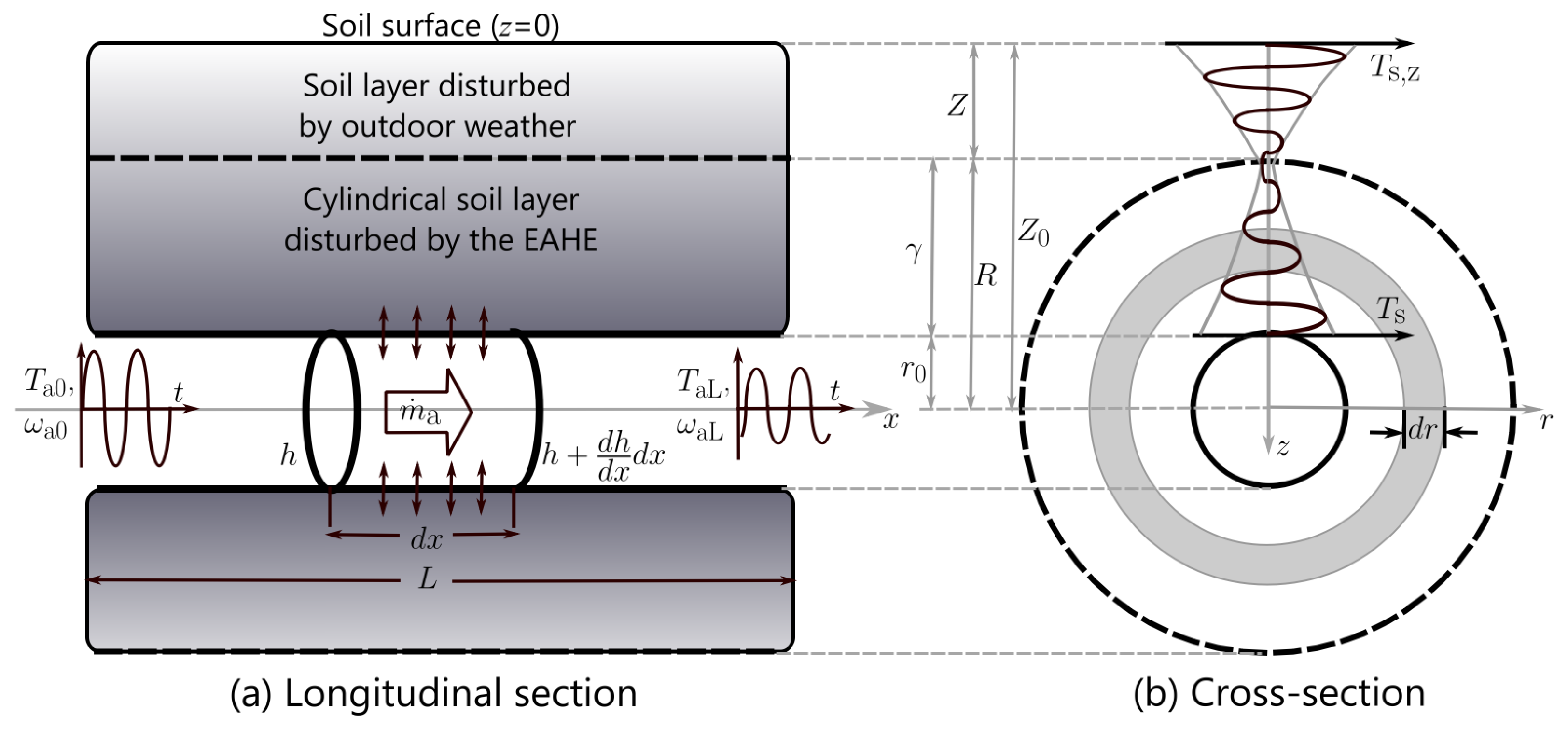
Figure 1 depicts the longitudinal section and cross-section of a cylindrical single-pipe large-diameter EAHE with radius $r_0$ and length L buried at depth $Z_0$.

As the mass flow rate ${\dot{m}}_{\mathrm{a}}$ of outdoor air flows inside the EAHE, heat and moisture transfer processes take place between air and soil. Since the outdoor air temperature ($T_{\mathrm{a}0}$) and moisture content (${\omega }_{a0}$) oscillate over the course of the day (and also throughout the year), the disturbance introduced by the EAHE is limited to a cylindrical soil layer of length $\gamma$ surrounding the EAHE [55,56]. Because the surface of the soil is exposed to the outdoors, the soil temperature $T_{\mathrm{s},\mathrm{z}}$ above the EAHE is also a function of dynamic weather conditions.

To highlight the numerous transient factors influencing heat and mass transfer in the EAHE, Figure 1a includes sketches depicting the oscillatory nature of air temperature and moisture content (expressed as humidity ratio, $\omega$) when air enters and exits the EAHE. Subscripts a0 and aL are used to distinguish both cases. Moreover, Figure 1b sketches the “thermal waves” and temperature amplitudes in the cylindrical layer $r_0\le r<$ R—disturbed mainly by the presence of the EAHE—and in the soil layer $0\le z<$ Z—disturbed mainly by outdoor weather.

Regarding these “thermal waves”, and according to [56], for ground depths of approximately 0.3 m, the effect on $T_{\mathrm{s},\mathrm{z}}$ of daily variations in weather conditions becomes negligible; for larger depths, the effect of seasonal weather variations is significantly dampened. Indeed, for a distance to the soil surface larger than 3 m, the soil temperature amplitude becomes small [20,33,57], and, when studying EAHEs, for these depths, the soil temperature can be approximated by the annual average of outdoor air temperatures; i.e., $T_{s,z}\approx {\overline{T}}_{\mathrm{a}0}$ if $z\ge Z$, with Z defining the soil depth for which the seasonal changes in outdoor conditions are significantly dampened [55].

In this paper it is assumed that the soil’s temperature along the surface of the cylinder of radius $R(=r_0+\gamma )$ surrounding the EAHE remains approximately constant in time (t) and equal to the average annual temperature ${\overline{T}}_{\mathrm{a}0}$. The cylindrical soil layer limited between radii $r_0$ and R surrounding the EAHE is, therefore, disturbed chiefly by the heat and mass transfer processes occurring in the EAHE. The soil temperature in this layer is identified as $T_{\mathrm{s}}$.

Anticipating the mathematical formulation presented in the next subsections, domains of air with radius $r_0$ and infinitesimal length $dx$, of soil with infinitesimal radii $dr$, as well as the change in a property of air (specific enthalpy, h) along $dx$ are also depicted in Figure 1.

2.2. Air Moisture Mass Conservation Equation

As outdoor air flows inside the EAHE its moisture content can condense on the pipe surface, or water can evaporate from this surface, changing the moisture content of the airflow. The conservation of moisture in an infinitesimal cylinder of air, such as the one in Figure 1a, can be expressed as

$${\displaystyle \frac{{\dot{m}}_{\mathrm{a}}}{v_{\mathrm{a}}}}{\displaystyle \frac{\partial \omega }{\partial t}}+{\dot{m}}_{\mathrm{a}}{\displaystyle \frac{\partial \omega }{\partial x}}+2\pi r_0{S}_{\omega }=0,$$

(1)

where $\omega$ is the humidity ratio, $v_{\mathrm{a}}$ is the airflow velocity, and the source term $S_{\omega }$ accounts for moisture condensation on/water evaporation from the inner EAHE surface (of radius $r_0$). This source term is defined as

$$S_{\omega }=\Gamma h_m\left(\omega -{\omega }_{\mathrm{sat}}{|}_{T_{\mathrm{s}\left|\mathrm{r}0\right.}}\right),$$

(2)

using ${\omega }_{\mathrm{sat}}{|}_{T_{\mathrm{s}\left|\mathrm{r}0\right.}}$ to express the humidity ratio of saturated moist air at the inner EAHE wall temperature, $T_{\mathrm{s}}{|}_{\mathrm{r}0}$. Hence, condensation/evaporation of moisture is related to the “degree of saturation” (to the ratio $\omega /{\omega }_{\mathrm{sat}}{|}_{T_{\mathrm{s}\left|\mathrm{r}0\right.}}$) being larger/smaller than one. Additional parameters in Equation (2) are $h_m$, a mass transfer coefficient at the EAHE inner surface, and $\Gamma$, an effective area coefficient of mass transfer (which is assumed constant and equal to 1).

To determine the mass transfer coefficient, the Lewis formula is used,

$$h_{\mathrm{m}}={\displaystyle \frac{h_{\mathrm{a}}}{c_{\mathrm{p},\mathrm{a}}}}F\left(Le\right),$$

(3)

with $F\left(Le\right)$ the Lewis function (also taken as constant and equal to 1), $c_{\mathrm{p},\mathrm{a}}$ the specific heat capacity of air, and $h_{\mathrm{a}}$ the heat transfer coefficient at the EAHE inner surface; in this paper, determined from [55],

$$h_a={\displaystyle \frac{{\lambda }_a}{2r_0}}Nu$$

(4a)

with ${\lambda }_a$ the thermal conductivity of air,

$$Nu=4.36,\mathrm{for}\mathrm{laminar}\mathrm{flow}(Re<2300),$$

(4b)

$$Nu=0.023R{e}^{0.8}P{r}^{0.33}\mathrm{for}\mathrm{turbulent}\mathrm{flow}(Re>10,000),$$

(4c)

and using values of Nu interpolated from the expressions above when 2300 ≤ Re ≤ 10,000.

To determine the mass of moisture that condenses/is added to the air flowing in the EAHE, Equation (1) requires integration along time t and along the longitudinal x direction of the EAHE. The boundary and initial conditions considered are

$$\omega (0,t)={\omega }_{\mathrm{a}0}\left(t\right),$$

(5)

and

$$\omega (x,0)={\omega }_{\mathrm{a}0}\left(0\right).$$

(6)

Still, to solve Equation (1), time and longitudinal distributions for the EAHE inner surface temperature $T_{\mathrm{s}}{|}_{r_0}$ are required, and this calls for energy conservation equations.

2.3. Energy Conservation Equations

The first energy conservation equation to consider is that of heat diffusion in the soil applied to the infinitesimal radial domain depicted in Figure 1b.

$${\displaystyle \frac{\partial T_s}{\partial t}}-{\alpha }_s\left({\displaystyle \frac{{\partial }^2{T}_s}{\partial r^2}}+{\displaystyle \frac{1}{r}}{\displaystyle \frac{\partial T_s}{\partial r}}\right)=0.$$

(7)

This equation provides the temperature $T_{\mathrm{s}}{|}_{r_0}$ required to solve the mass balance introduced in the previous section, with ${\alpha }_s$ representing the soil thermal diffusivity.

To find a solution to Equation (7) the following boundary and initial conditions apply.

• Boundary condition at $r=R$:

  $${T_{\mathrm{s}}|}_R=T_{\mathrm{s},\mathrm{Z}},$$

  (8)

  assuming the soil temperature at the most distant radius $r=R$ is equal to the undisturbed soil temperature at depth Z.
• Boundary condition at $r=r_0$:

  $$-{\lambda }_s{\displaystyle \frac{\partial T_{\mathrm{s}}}{\partial r}}{|}_{r_0}=h_a\left(T_a-T_{\mathrm{s}}{|}_{r_0}\right)+L_{\mathrm{v}}{S}_{\omega },$$

  (9)

  with ${\lambda }_s$ the soil thermal conductivity and $L_{\mathrm{v}}$ the latent heat of vaporization of water. Given that this boundary condition requires a link between the density of heat conducted to/from the soil and the density of sensible and latent heat transferred from/to the flow of moist air, an additional conservation equation is required to determine air temperatures.
• Initial condition at $t=0$:

  $$T_s(r,x,0)=T_{\mathrm{s},\mathrm{Z}},$$

  (10)

  assuming, for $t=0$, a homogeneous soil temperature around the EAHE pipe equal to the temperature of the undisturbed soil at depth Z.

The second energy conservation equation relates air temperature advection with air–soil heat transfer in the infinitesimal cylindrical domain of air depicted in Figure 1a. This equation is expressed as

$${\displaystyle \frac{{\dot{m}}_{\mathrm{a}}}{v_{\mathrm{a}}}}{\displaystyle \frac{\partial h}{\partial t}}+{\dot{m}}_{\mathrm{a}}{\displaystyle \frac{\partial h}{\partial x}}+2\pi r_0\left[h_{\mathrm{a}}\left(T_{\mathrm{a}}-T_{\mathrm{s}}{|}_{r_0}\right)\right]+L_{\mathrm{v}}{S}_{\omega }=0,$$

(11)

with h the specific enthalpy of moist air.

Equation (11) is simplified, expressing the specific enthalpy of moist air as

$$h=c_{p,a}{T}_a+\left(c_{p,v}{T}_a+L_{\mathrm{v}}\right)\omega ,$$

(12)

a function of air temperature and air humidity ratio ($c_{\mathrm{p},\mathrm{v}}$ being the specific heat capacity of water vapor).

Replacing Equation (12) in (11) and rearranging the following expression, we obtain

$$\begin{array}{c}\hfill \left(c_{\mathrm{p},\mathrm{a}}+c_{\mathrm{p},\mathrm{v}}\omega \right){\displaystyle \frac{{\dot{m}}_{\mathrm{a}}}{v_{\mathrm{a}}}}{\displaystyle \frac{\partial T_a}{\partial t}}+\left(c_{\mathrm{p},\mathrm{a}}+c_{\mathrm{p},\mathrm{v}}\omega \right){\dot{m}}_{\mathrm{a}}{\displaystyle \frac{\partial T_a}{\partial x}}+2\pi r_0{h}_{\mathrm{a}}\left(T_{\mathrm{a}}-T_{\mathrm{s}}{|}_{r_0}\right)=\\ \hfill -\left[\left(c_{\mathrm{p},\mathrm{v}}{T}_a+L_{\mathrm{v}}\right){\displaystyle \frac{{\dot{m}}_{\mathrm{a}}}{v_{\mathrm{a}}}}{\displaystyle \frac{\partial \omega }{\partial t}}+\left(c_{\mathrm{p},\mathrm{v}}{T}_a+L_{\mathrm{v}}\right){\dot{m}}_{\mathrm{a}}{\displaystyle \frac{\partial \omega }{\partial x}}+2\pi r_0{L}_{\mathrm{v}}{S}_{\omega }\right].\end{array}$$

(13)

Because, for typical EAHE applications, the latent heat of vaporization $L_{\mathrm{v}}$ exceeds $c_{p,v}{T}_a$ by two orders of magnitude, the approximation $\left(c_{p,v}{T}_a+L_v\right)\simeq L_{\mathrm{v}}$ applies, and, after factoring out $L_{\mathrm{v}}$ on the right member and using the moisture mass balance equation (Equation (1)), the right member of Equation (13) becomes zero.

Moreover, because, for typical EAHE applications, $c_{\mathrm{p},\mathrm{a}}$ is also two orders of magnitude larger than $c_{\mathrm{p},\mathrm{v}}\omega$, the approximation $\left(c_{\mathrm{p},\mathrm{a}}+c_{\mathrm{p},\mathrm{v}}\omega \right)\simeq c_{\mathrm{p},\mathrm{a}}$ applies, and the following simplified expression relating air temperature advection inside the EAHE to air–soil heat transfer is obtained,

$${\dot{m}}_{\mathrm{a}}{c}_{\mathrm{p},\mathrm{a}}\left({\displaystyle \frac{1}{v_{\mathrm{a}}}}{\displaystyle \frac{\partial T_a}{\partial t}}+{\displaystyle \frac{\partial T_a}{\partial x}}\right)+2\pi r_0{h}_{\mathrm{a}}\left(T_{\mathrm{a}}-T_{\mathrm{s}}{|}_{r_0}\right)=0.$$

(14)

Boundary and initial conditions for Equation (14) are:

• Boundary condition at $x=0$:

  $$T_a(0,t)=T_{\mathrm{a}0}\left(t\right),$$

  (15)

  because outdoor air enters the EAHE.
• Initial condition at $t=0$:

  $$T_a(x,0)=T_{\mathrm{s},\mathrm{Z}},$$

  (16)

  assuming, for $t=0$, uniform air temperature inside the EAHE equal to the temperature of the undisturbed soil.

The set of Equations (1), (7) and (14) together with boundary and initial conditions (5), (6), (8), (9), (10), (15) and (16) specify the complete coupled heat and moisture transfer process in an EAHE.

2.4. Numerical Implementation

The set of partial differential equations (PDEs) subject to the boundary and initial conditions introduced in the previous section were solved numerically using the method of lines (MOL). This method transforms the PDE problem into an ordinary differential equation (ODE) problem discretizing the space variables x and r.

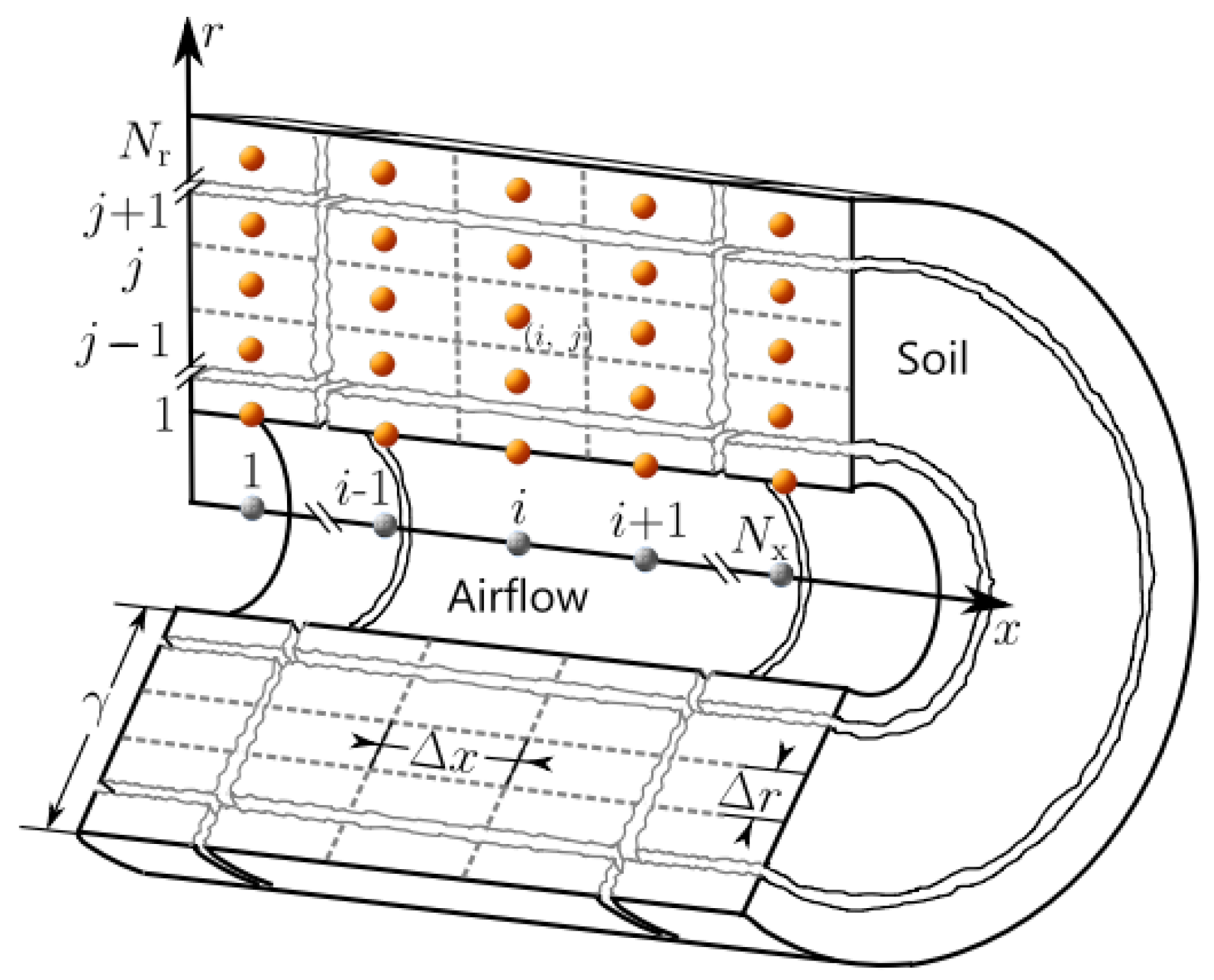
The finite difference method was applied, and Figure 2 presents a sketch of a mesh discretizing the soil in the radial r direction around an EAHE and also representing positions along the x direction to discretize the path along which moist air (assumed well mixed) flows inside the EAHE from the inlet to the outlet. The number of points in the soil and along the EAHE longitudinal direction is defined by $N_r$ and $N_x$, respectively, with $\Delta r$ and $\Delta x$ representing the distance between two consecutive points in the radial and longitudinal directions, respectively.

Using the nomenclature presented in Figure 2, discretized versions of Equations (1), (7) and (14) are

$${\dot{m}}_{\mathrm{a}}{\displaystyle \frac{1}{v_{\mathrm{a}}}}{\displaystyle \frac{\partial {\omega }_i}{\partial t}}=-{\dot{m}}_{\mathrm{a}}{\displaystyle \frac{{\omega }_i-{\omega }_{i-1}}{\Delta x}}-2\pi r_0{S}_{\omega ,i},$$

(17)

$${\displaystyle \frac{\partial T_{s,i,j}}{\partial t}}={\alpha }_s\left({\displaystyle \frac{T_{s,i,j+1}-2T_{s,i,j}+T_{s,i,j-1}}{{\left(\Delta r\right)}^2}}+{\displaystyle \frac{1}{r_j}}{\displaystyle \frac{T_{s,i,j+1}-T_{s,i,j}}{\Delta r}}\right),$$

(18)

$${\dot{m}}_{\mathrm{a}}{c}_{\mathrm{p},\mathrm{a}}{\displaystyle \frac{1}{v_{\mathrm{a}}}}{\displaystyle \frac{\partial T_{a,i}}{\partial t}}=-{\dot{m}}_{\mathrm{a}}{c}_{\mathrm{p},\mathrm{a}}{\displaystyle \frac{T_{a,i}-T_{a,i-1}}{\Delta x}}-2\pi r_0{h}_{\mathrm{a}}\left(T_{\mathrm{a},\mathrm{i}}-T_{\mathrm{s},\mathrm{i},1}\right).$$

(19)

The applicable boundary and initial conditions become

$$-{\lambda }_s{\displaystyle \frac{T_{s,i,2}\left(t\right)-T_{s,i,1}\left(t\right)}{\Delta r}}=h_a\left(T_{a,i}\left(t\right)-T_{s,i,1}\left(t\right)\right)+L_{\mathrm{v}}{S}_{\omega ,i}\left(t\right).$$

(20)

$$T_{s,i,N_{\mathrm{r}}}\left(t\right)=T_{\mathrm{s},\mathrm{Z}},$$

(21)

$$T_{a,1}\left(t\right)=T_{\mathrm{a}0}\left(t\right),$$

(22)

$${\omega }_1\left(t\right)={\omega }_{\mathrm{a}0}\left(t\right).$$

(23)

and

$$T_{s,i,j}(t=0)=T_{\mathrm{s},\mathrm{Z}},$$

(24)

$$T_{a,i}(t=0)=T_{\mathrm{s},\mathrm{Z}},$$

(25)

$${\omega }_i(t=0)={\omega }_{\mathrm{a}0}\left(0\right),$$

(26)

with $i=1,2,\dots ,N_x$ and $j=1,2,\dots ,N_r$.

This set of ordinary differential equations together with the boundary conditions form a system of differential–algebraic equations that, once integrated with the initial conditions, produce the numerical solution to the coupled heat and moisture mass transfer problem in an EAHE.

This system of equations was solved using the linearly implicit Rosenbrock 2(3) method, originally introduced by Rosenbrock [58] and later formalized within the Rosenbrock Wanner class of solvers [59]. Convergence tolerances were set to 10⁻³ for the relative error and 10⁻⁶ for the absolute error. The embedded third-order estimator [60] provides robust adaptive time step control, enabling the solver to automatically adjust the time step based on the estimated local truncation error at each iteration. This approach has been shown to be efficient and reliable for stiff systems arising from the method of lines discretization of PDEs [61].

To study the grid independence of the numerical results, analytical solutions available in the literature were used. The analytical result provided by Hollmuller [55] was one of the selected solutions as it enables the assessment of sensible heat transfer due to convection between the air and the inner surface of the EAHE, as well as heat transfer by conduction from this surface into the surrounding soil. The analytical solution expressing the adiabatic cooling of the air flowing through the EAHE was also considered, thereby allowing the evaluation of latent heat transfer associated with the moisture phase-change process.

To assess the numerical errors, the root-mean-square of relative error (RMSRE, expressed as a percentage) was used,

$$RMSRE\left(y\right)=\sqrt{{\displaystyle \frac{1}{n}}\sum _{k=1}^n{\left({\displaystyle \frac{y^{\mathrm{num}}\left(k\right)-y^{\mathrm{analyt}\mathrm{or}\mathrm{monit}}\left(k\right)}{y^{\mathrm{analyt}\mathrm{or}\mathrm{monit}}\left(k\right)}}\right)}^2},$$

(27)

where the superscripts “num” and “analyt” refer to the numerical results and analytical solution, respectively, for the property y under comparison, and n denotes the number of discretized points (RMSRE will also be used to compare numerical results with monitoring data, hence the inclusion of the superscript “monit”).

For the validation of the computational model, the design and operating parameters of a large-diameter EAHE currently in use were adopted as the reference case.

Table 1. Reference values of geometric, installation (depth), operational and thermophysical parameters used to assess the convergence and validate the use of the computational model.

Parameter Type	Reference (or Nominal) Value
Geometry/Installation (depth)	$L=70$ m
	$r_0=0.5$ m
	$Z_0=5.5$ m
Operational	$\dot{V}=4000$ m3/h = 1.(1) m3/s
	$v_{\mathrm{a}}=1.415$ m/s (from $\dot{V}$ and $r_0$)
	${\overline{T}}_{\mathrm{a}0}=T_{\mathrm{s},\mathrm{Z}}=20$ °C
Thermophysical	$c_{\mathrm{p},\mathrm{a}}=1005$ J/(kg K)
	$c_{\mathrm{p},\mathrm{v}}=1860$ J/(kg K)
	$L_{\mathrm{v}}=2501\times {10}^3$ J/kg
	${\rho }_{\mathrm{a}}=1.2$ kg/m3
	${\alpha }_{\mathrm{s}}=1\times {10}^{-6}$ m2/s

presents these reference values. Section 2.6 (and Ref. [19]) provide more details about the studied EAHE.

2.5. Validation of the Numerical Model Using Analytical Solutions

2.5.1. Case 1: Comparison with the Analytical Solution for the EAHE Exit Air Temperature

Hollmuller’s analytic solution [55] was used to test the grid independence of the numerical results considering sensible heat transfer in the EAHE and outdoor air temperature oscillating with known amplitude and frequency.

The EAHE parameters specified in Table 1 were used to develop the computational model, and it was assumed that the outdoor air temperature varied throughout the day according to the expression $T_{a0}\left(t\right)={\overline{T}}_{a0}+{\theta }_{a0}cos\left[{\displaystyle \frac{2\pi }{T}}\left(t-17\right)+\phi \right]$, with ${\overline{T}}_{a0}=25$ °C, ${\theta }_{\mathrm{a}0}=10$ °C, $T=$ 24 h and φ = 0 rad.

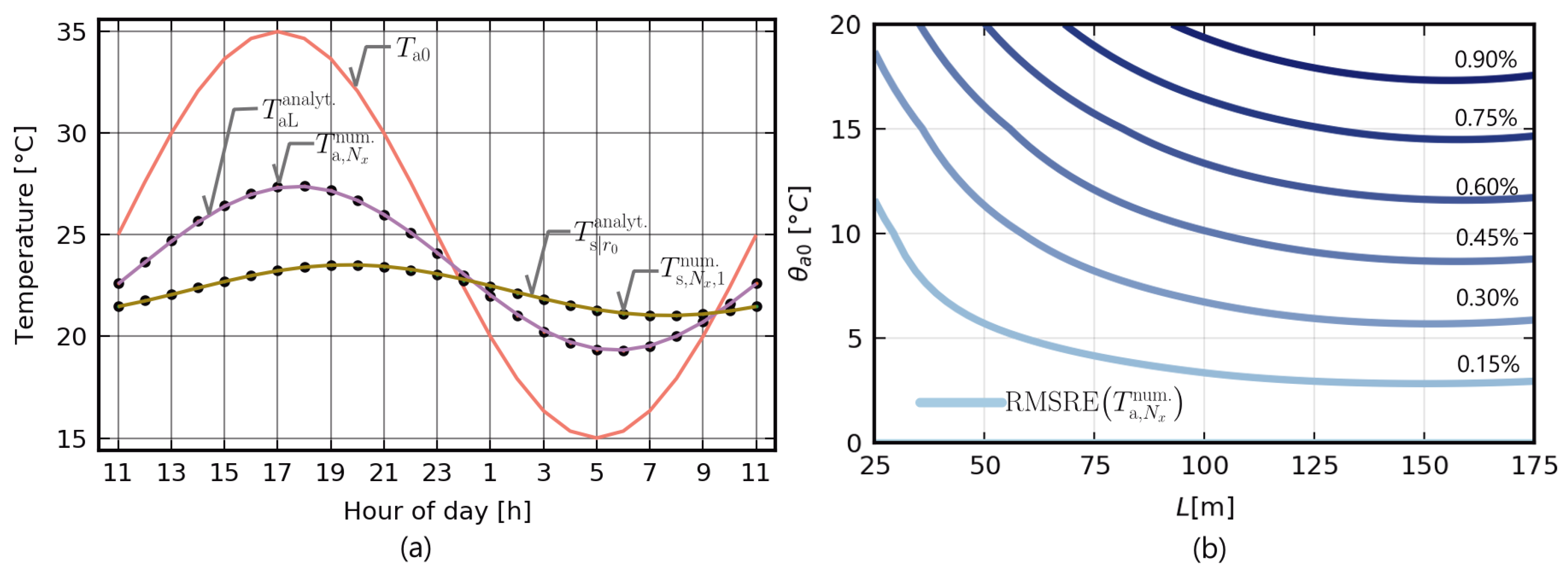
For the 24 h period of oscillation, Figure 3a presents the sinusoid describing the outdoor air temperature, as well as the sinusoids for the analytical solution and numerical results for (i) air temperature exiting the EAHE, $T_{\mathrm{a},N_x}$, and (ii) EAHE inner surface temperature when $x=L=70$ m; i.e., at the EAHE exit, $T_{\mathrm{s},N_x,1}$.

A good agreement between the numerical results (black dots) and the analytical solutions (solid lines) is visible in Figure 3a. The results highlight the $2.5$ °C reduction in the mean air temperature between EAHE inlet, with ${\overline{T}}_{\mathrm{a}0}=25$ °C, and EAHE outlet, with ${\overline{T}}_{\mathrm{aL}}=22.5$ °C (from Table 1, the reference undisturbed soil temperature is $T_{\mathrm{s},\mathrm{Z}}=20$ °C). Moreover, between EAHE inlet and outlet, air temperature amplitude is dampened by half, from 10 °C to 5 °C, and a phase shift $\phi$ of approximately 1 h is noticeable. Larger reductions in temperature mean, amplitude dampening and phase shift are obtained for the EAHE inner surface temperature results, $T_{\mathrm{s},N_x,1}$.

Since the mean temperature reduction, amplitude dampening and the phase shift vary with outdoor air conditions and with the geometry of the EAHE using the $N_x=21$ and $N_r=33$ mesh but considering different EAHE lengths L and outdoor temperature amplitudes ${\theta }_{\mathrm{a}0}$, Figure 3b presents RMSRE contour lines for EAHE exit air temperatures. These contour lines were obtained using Equation (27) with $y^{\mathrm{num}.}\left(k\right)=T_{\mathrm{a},\mathrm{i}=N_x}^{\mathrm{num}.}\left(k\right)$, $y^{\mathrm{analyt}.}\left(k\right)=T_{\mathrm{a},\mathrm{x}=\mathrm{L}}^{\mathrm{analyt}.}\left(k\right)$, and $k=1,2,\dots ,24$ the hour of day ($n=24$).

Figure 3b shows that the relative errors in the numerical results increase for larger EAHE lengths and for larger outdoor air temperature amplitudes. However, when the EAHE length exceeds approximately 125 m, the relative errors become independent of the EAHE length and depend solely on the thermal amplitude of the outdoor air. From a quantitative standpoint, Figure 3b shows that, for the conditions studied, the RMSRE values of the numerical results are consistently below 1%.

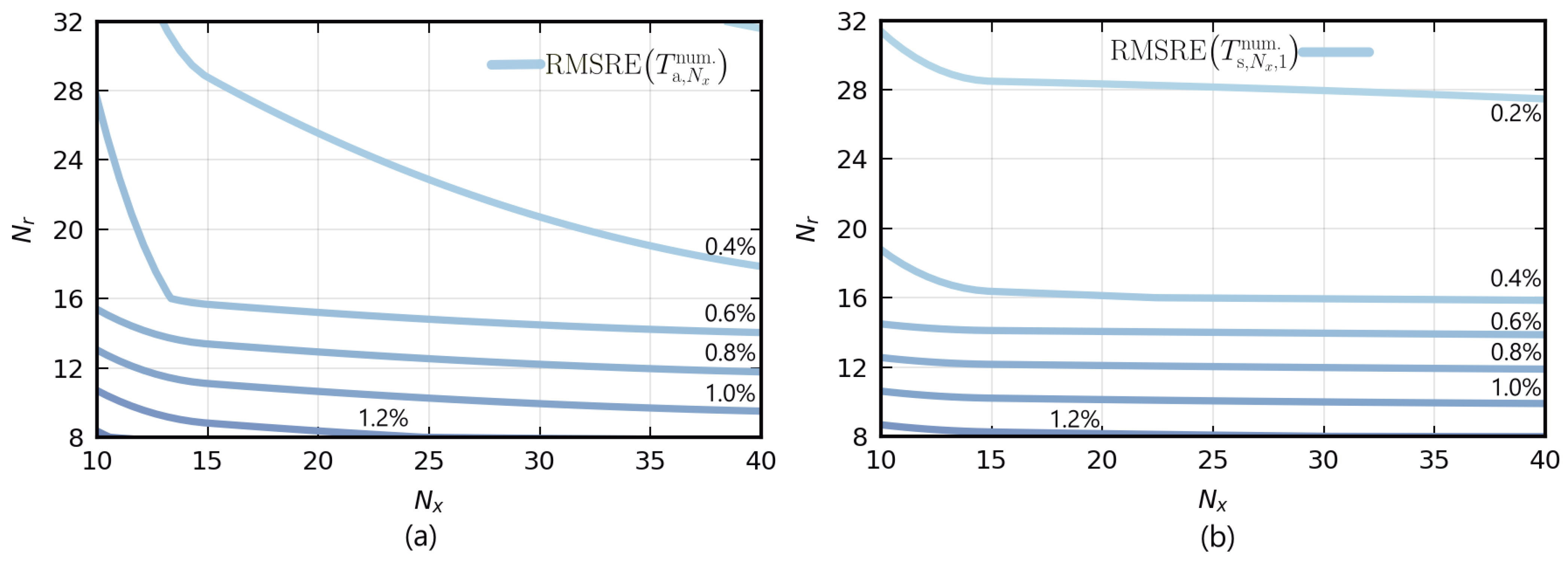
To assess how numerical errors vary with grid discretization, Figure 4 depicts, for the reference EAHE and different values of $N_x$ and $N_r$, contour lines of RMSRE (percentages; again with $k=1,2,\dots ,n$ and $n=24$) for the EAHE exit air temperature, $T_{\mathrm{a},N_x}$, and inner surface temperature at the end of the EAHE, $T_{\mathrm{s},N_x,1}$.

Figure 4 shows that, for finer meshes with larger $N_x$ and $N_r$ (lower $\Delta x$ and $\Delta r$, respectively), the numerical results approach the analytical solution. Indeed, for $N_x=21$ and $N_r\ge 21$, the RMSRE values are always below 0.5%. Figure 4 also shows that increased numerical precision requires larger discretization along the radial direction r but is rather insensitive to the discretization along the longitudinal x direction.

The results from Figure 3 and Figure 4 confirm the ability the computational model has to correctly determine the sensible/convective heat transfer from air to the EAHE inner surface and from there to the soil even if relatively coarse meshes are used.

2.5.2. Case 2: Comparison with the Analytic Solution for the Adiabatic Cooling of Air Flowing in the EAHE

To confirm the ability the computational model has to correctly determine latent heat transfer, numerical results were compared with the analytical solution for the case of adiabatic cooling of air flowing in the EAHE.

To model adiabatic cooling of air, the inner surface of the EAHE is assumed adiabatic and wet with a known constant saturated humidity ratio, ${\omega }_{\mathrm{sat}}{|}_{T_{\mathrm{s}\left|\mathrm{r}0\right.}}$, and the humidity ratio of air entering the EAHE, ${\overline{\omega }}_{\mathrm{a}0}$, is also assumed constant. In this case, the increase/decrease in moisture along the longitudinal direction of the EAHE is accompanied by the decrease/increase in air temperature, and the analytical solution for the humidity ratio distribution along the EAHE is given by

$$\omega \left(x\right)={\omega }_{\mathrm{sat}}{|}_{T_{\mathrm{s}\left|\mathrm{r}0\right.}}+\left({\overline{\omega }}_{\mathrm{a}0}-{\omega }_{\mathrm{sat}}{|}_{T_{\mathrm{s}\left|\mathrm{r}0\right.}}\right)e^{-Kx},$$

(28)

with

$$K={\displaystyle \frac{2\pi r_0{h}_{\mathrm{a}}}{{\dot{m}}_{\mathrm{a}}{c}_{\mathrm{p},\mathrm{a}}}}.$$

(29)

Considering the reference EAHE, with ${\omega }_{\mathrm{sat}}{|}_{T_{\mathrm{s}\left|\mathrm{r}0\right.}}={\omega }_{\mathrm{sat}}{|}_{T_{\mathrm{s}\left|\mathrm{Z}\right.}}$ and ${\overline{\omega }}_{\mathrm{a}0}=0.60\left({\omega }_{\mathrm{sat}}{|}_{T_{\mathrm{s}\left|\mathrm{r}0\right.}}\right)$, a summer design condition,

Table 2. RMSRE results for ${\omega }_{\mathrm{i}}$ with $i=1,2,\dots ,N_x$ considering adiabatic cooling of air in the reference EAHE.

${\mathit{N}}_{\mathit{x}}$	11	21	41
RMSRE(${\omega }_{\mathrm{i}}$) [%]	$2\times {10}^{-7}$	$4\times {10}^{-9}$	$9\times {10}^{-11}$

presents RMSRE values (in percentage) considering different discretizations along the longitudinal x direction. RMSRE values are determined from Equation (27) with $y^{\mathrm{num}.}\left(k\right)={\omega }_{\mathrm{i}=\mathrm{k}}$, $y^{\mathrm{analyt}.}={\omega }_{\mathrm{x}=\mathrm{k}}$, and $k=1,2,\dots ,N_x$ ($n=N_x$).

Table 2 highlights the agreement between the numeric results and the analytic solution, even when a relatively coarse mesh is used.

For the analytic solutions described in Case 2 and Case 1, the RMSRE results presented in this section confirm the ability the numerical model has to correctly determine the latent and sensible heat transfer processes occurring in an EAHE. The numerical results presented in the following sections are obtained using the spatial discretization with $N_r=33$ and $N_x=21$, which was found to be sufficiently accurate.

2.6. Validation of the Numerical Model Using Monitoring Data

For the validation of the numerical model, monitoring data were used from an EAHE currently in operation serving a small office building with a total floor area of 750 m² (60% of which is cooled), located near Beja, in the Alentejo region of Portugal. The EAHE consists of two 70-meter-long concrete pipes with a diameter of 1 m, placed 4 m apart (distance between axes) and buried 5.5 m deep (average depth since the pipes are sloped towards the air intake for water drainage). The nominal airflow rate is 4000 m³/h per pipe, or 8000 m³/h in total for both pipes, which can increase up to a maximum total airflow rate of 16,000 m³/h.

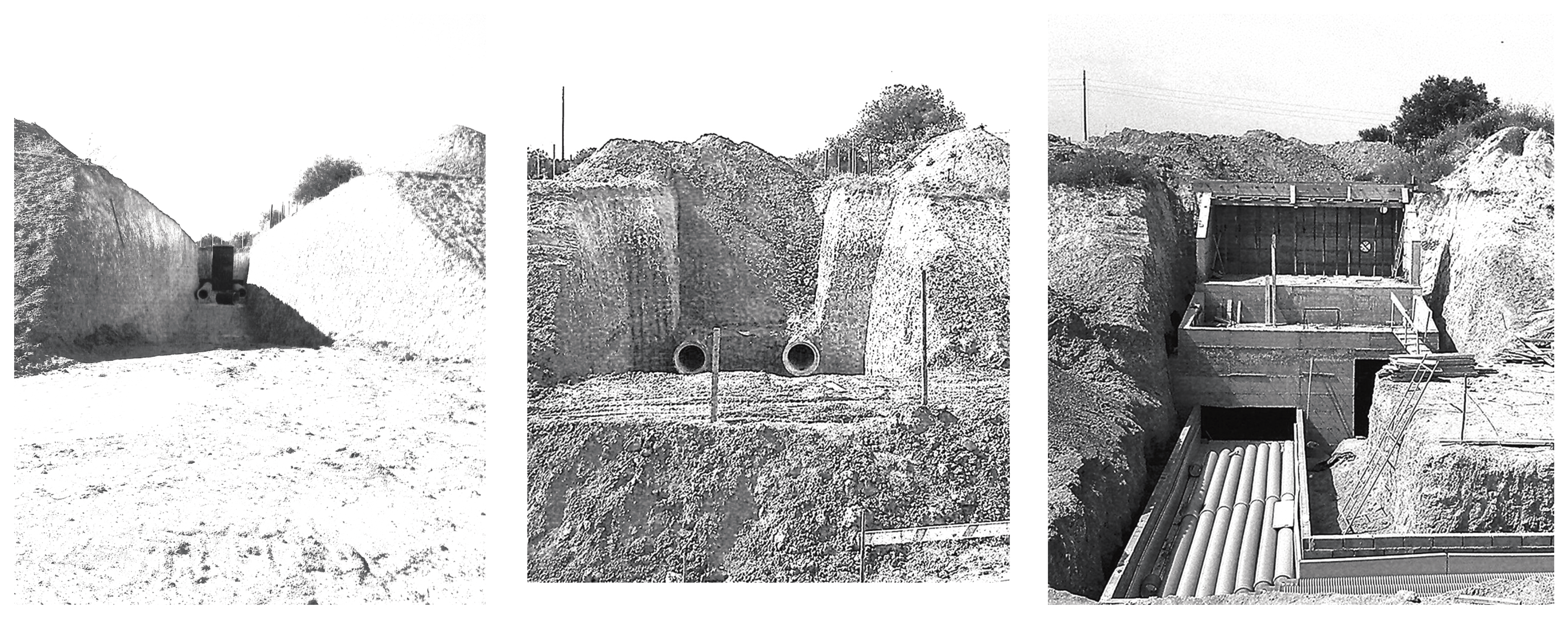
Figure 5 presents photographs of the EAHE at different construction stages: (from left to right) an initial stage with the trench for the pipes already opened and the air intake and initial sections of the pipes in place; an intermediate stage with the 70-meter-long pipes already in place and the trench filled with soil (only the two pipes’ exit sections are visible), and a subsequent stage with a technical space (downwind of the pipes) being built that is used to hold an AHU, an outdoor bypass section (not visible) and all the necessary equipment to control the operation of the EAHE. This last photograph also shows the corrugated pipes delivering the air to the office rooms. The paper by Duarte et al. [19] provides a schematic diagram detailing the components and mode of operation of the monitored EAHE as well as details on the office building being cooled.

To gather the monitoring data, a weather station [62] placed outdoors and temperature and relative humidity sensors installed at the end of the buried pipes [63] measured timeseries of outdoor air (i.e., EAHE inlet air) and EAHE exit air temperature and relative humidity. Further details concerning the monitoring process and sensor specifications are also provided in [19].

Since the EAHE pipes are impervious to water, moisture transfer between the soil and the air flowing inside the EAHE is neglected. Moreover, since moisture condensation occurring on the EAHE inner surface is presumed collected at the pipe bottom and drained out of the EAHE without evaporating, the source term $S_{\omega }$ becomes

$$S_{\omega }=\{\begin{array}{lll}& 0& \omega <{\omega }_{\mathrm{s}\mathrm{a}\mathrm{t}}{|}_{T_{\mathrm{s}|\mathrm{r}0}}\\ \Gamma h_m(\omega -{\omega }_{\mathrm{s}\mathrm{a}\mathrm{t}}{|}_{T_{\mathrm{s}|\mathrm{r}0}})& \omega \ge {\omega }_{\mathrm{s}\mathrm{a}\mathrm{t}}{|}_{T_{\mathrm{s}|\mathrm{r}0}}& \end{array}$$

(30)

Equation (30) implies that moisture evaporation is negligible compared to moist condensation, an assumption deemed reasonable.

Using Equation (30) to replace Equation (2) and introducing this change in the numerical implementation described in Section 2.4, a computational model capable of describing the behavior of the monitored EAHE was obtained. Since the geometry, nominal operating conditions and thermophysical parameters that apply to the monitored EAHEs are the reference conditions already used in Section 2.5, Table 1, the numerical discretization method and ODE problem solution method used in the previous section were also applied in this section. The main difference lies, therefore, in the use of the outdoor air monitoring (timeseries) data.

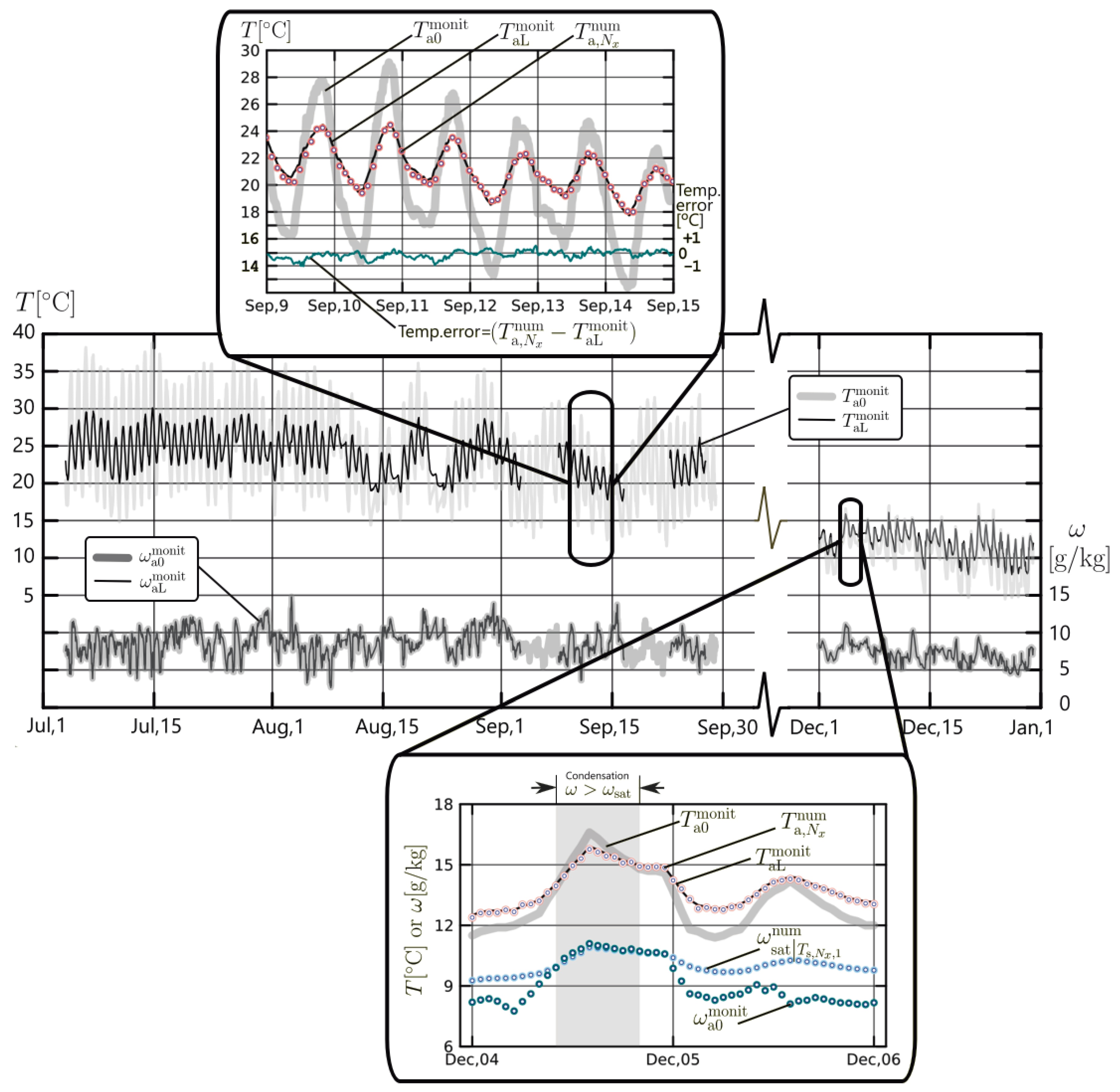
The center graph in Figure 6 presents monitored timeseries for EAHE exit air temperature and humidity ratio, $T_{\mathrm{aL}}^{\mathrm{monit}}$ and ${\omega }_{\mathrm{aL}}^{\mathrm{monit}}$. To characterize the meteorological conditions where the EAHE is located and to allow the discussion of the EAHE cooling performance, monitored timeseries of outdoor air temperature and humidity ratio (entering the EAHE) are also presented, $T_{\mathrm{a}0}^{\mathrm{monit}}$ and ${\omega }_{\mathrm{a}0}^{\mathrm{monit}}$.

The monitored EAHE was used for office cooling, so timeseries in Figure 6 describe the operation of the EAHE between July and September. During these summer months there were periods when cooling was not needed and the EAHE was turned off. For these periods (noticeable in September when outdoor temperature minima falls below 15 °C), timeseries of EAHE exit air temperature and humidity ratio are interrupted. With the specific objective of studying the occurrence of condensation in the EAHE, data for the month of December is also included in Figure 6.

The analysis of monitored data shows that, during the summer months, the EAHE significantly reduces the daily outdoor temperature amplitude. During the hottest hours of the day the EAHE decreased outdoor temperature maxima by up to approximately 9 °C, from ∼40 to ∼30 °C. In December, the decrease in daily outdoor temperature amplitude is smaller; still, for the coldest hours of the day, the EAHE increases the outdoor temperature minima by up to approximately 4 °C.

The inset above the main chart in Figure 6 provides a detail comparing monitored data with numerical results for a week in September. This detail confirms the agreement between the numerical results and the monitored data for the air temperature at the EAHE exit. The agreement is highlighted by the temperature error line, $E=T_{\mathrm{aL}}^{\mathrm{num}}-T_{\mathrm{aL}}^{\mathrm{monit}}$, whose scale is presented on the right vertical axis and whose magnitude never exceeds 1 °C.

Table 3. Error mean, standard deviation, minimum, maximum and RMSRE values for the air temperature numerical results presented in the top inset of Figure 6, between 9 September and 15 September, and for the whole summer, between July and September.

Temp. Error, E	Mean [°C]	Std [°C]	Min [°C]	Max [°C]	RMSRE [%]
9–15 September	−0.11	0.28	−0.90	0.59	1.45
July–September	−0.32	0.59	−2.89	2.44	2.90

presents statistics of this error, including the RMSRE of the numerical results for the period between 9 and 15 September. The table also includes the results for the entire summer period, from July to September.

The values presented in Table 3 demonstrate the agreement between the numerical results and the monitoring data for the air temperature at the EAHE exit, with the magnitudes of the mean and extreme values of the error E being lower than 0.5 °C and 3 °C, respectively, and with RMSRE values below 3%.

Regarding the timeseries of air humidity ratio, the center graph in Figure 6 shows no noticeable differences between monitored values for the outdoors (entering the EAHE) and monitored values at the EAHE exit. In other words, either no condensation occurs or, if it does, the associated reduction in humidity ratio is too small to be detected within the uncertainty of the measurements. Given the sensor accuracies ($\pm 0.35$ °C for temperature and ±5% for relative humidity), the relative uncertainty in the calculated humidity ratio may reach approximately $\pm 10\%$ under hot-weather conditions.

For the summer months, this absence of condensation is attributed to the characteristic hot and dry weather conditions where the EAHE is located. During the winter, the small difference between humidity ratio entering and exiting the EAHE is attributed to the large burial depth of the EAHE (5.5 m), and Beja’s relatively large undisturbed soil temperature at that depth ($17\sim 18.5$ °C).

The inset below the main chart in Figure 6 provides a detailed comparison of monitored data with numerical results for two days in December. In the region shaded in gray, the outdoor air temperatures are higher than 15 °C and also higher than the air outlet temperatures of the EAHE. Since the outdoor air enters the EAHE in a saturated state (as indicated by the values of the pair $T_{\mathrm{a}0}^{\mathrm{monit}}$, ${\omega }_{\mathrm{a}0}^{\mathrm{monit}}$), it can be concluded that condensation occurs within the shaded region. As mentioned above, the limited variation in the monitored humidity ratio data at the inlet and outlet of the EAHE does not allow the mass of condensed vapor to be quantified. Nevertheless, the detailed view includes values of the saturation humidity ratio corresponding to the EAHE surface temperature, obtained using the numerical model. As can be observed, these values are lower than those of the humidity ratio at the EAHE inlet, thereby confirming the numerical model’s ability to identify condensation. Since the difference ${\omega }_{\mathrm{a}0}^{\mathrm{monit}}-{\omega }_{\mathrm{sat}\left|T_{\mathrm{s},N_x,1}\right.}^{\mathrm{num}}$ is small, the mass of condensates determined numerically is also small.

2.7. Discussion of the Numerical Model Implementation and Validation

The comparison between the model results and monitoring data obtained from an EAHE in operation demonstrated the good agreement of the numerical results. Specifically:

• For a one-week period in September analyzed in detail in Figure 6, the root-mean-square relative error (RMSRE) of the numerical results for the air temperature at the outlet of the EAHE did not exceed 1.5%.
• Throughout the entire period analyzed in Figure 6, from July to September, the RMSRE of the numerical results for the air temperature at the EAHE outlet was 2.90%, with the mean and maximum absolute error values equal to 0.32 °C and 2.9 °C, respectively.
• With regard to the occurrence of condensation, it was shown that the numerical model correctly predicts its occurrence. However, given the dry summer climate and the operating conditions of the monitored EAHE, it was not possible to perform a quantitative comparison between the numerical results and monitoring records of the vapor mass that condenses inside the EAHE. Previous studies investigating the performance of EAHEs in hot and dry climates have also concluded that the occurrence of condensation is unlikely [18,38].

The good fit of the numerical results did not require highly refined meshes; indeed, in the grid-independence test of the numerical model, it was concluded, by comparison with analytical solutions, that

• Discretizations of 21 by 21 elements along the longitudinal and radial directions are sufficient to obtain RMSRE values below 0.5% when studying the sensible heat exchanges occurring in the EAHE;
• When studying adiabatic cooling in the EAHE by modeling latent heat exchanges with the discretization mentioned in the previous item, the numerical error becomes negligible.

In other words, despite the complexity of modeling the thermo-hygrometric phenomena occurring inside an EAHE, the mathematical formulation introduced in Section 2 and the SciML-based numerical implementation used in this article were successful, both in modeling the physical processes (convection, diffusion, and condensation) and in the selection of the geometric parameters and thermophysical properties (i.e., of the soil and air) that govern the coupled heat and mass transfer process in an EAHE.

The favorable validation results provide some assurance that the model can be used to evaluate the performance of EAHEs considering geometries and operating conditions different from those observed in the monitored EAHE. They thus enable a detailed analysis of EAHE operation in standalone cooling mode and a comparison of this mode with the more common precooling mode.

With the objective of assessing design solutions, climatic conditions, and soil characteristics best suited for EAHEs operating in standalone cooling mode, the following section employs the numerical model to perform a sensitivity analysis of cooling thermal loads with respect to different parameters affecting EAHE performance.

3. Investigating EAHE Use for Standalone Building Cooling

To investigate the use of EAHEs operating in standalone cooling mode, a metric must first be defined to evaluate the EAHE’s performance. The natural metric is the cooling capacity of the EAHE or, in other words, the capacity to remove thermal load from the air flowing through the EAHE. However, the accounting of the removed thermal load differs depending on whether the EAHE operates in standalone cooling mode or in precooling mode. The next section therefore begins by clarifying this difference.

3.1. Distinguishing Load Removal in Standalone Cooling and Precooling Modes of EAHE Operation

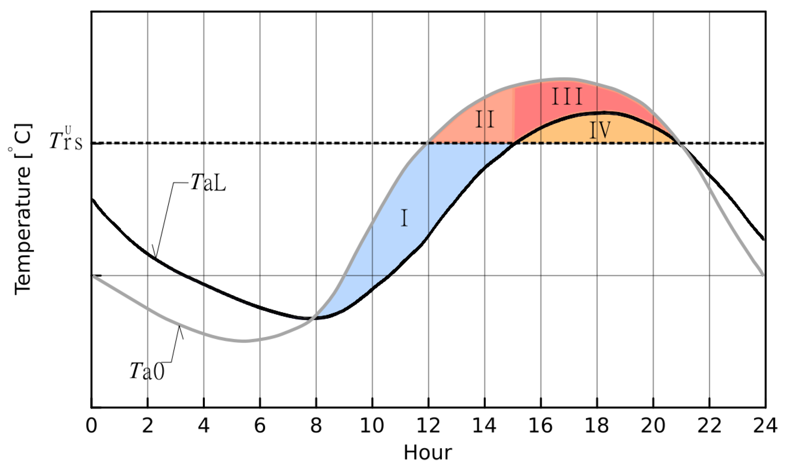
To highlight the differences between operating an EAHE for air precooling (used in a mechanical refrigerating system) and operating an EAHE used for standalone cooling, Figure 7 presents the 24 h evolution of air temperatures at the inlet and outlet of an EAHE (the effect of latent heat removal associated with condensation on the inner surface of the EAHE is neglected).

Figure 7 shows that the EAHE cools outdoor air between approximately 8:00 and 21:00, a period during which the air temperature at the EAHE exit is lower than the outdoor air temperature.

The (sensible) energy saved by the EAHE will be proportional to the areas represented in Figure 7 by I, II and III. Assuming the upper setpoint temperature in a room, $T_{\mathrm{rs}}^{\mathrm{U}}$, in order to cool the room, the supply air temperature must be lower than this value; consequently, for an EAHE system operating in precooling mode fitted with mechanical refrigeration, the refrigeration machine will need to remove the quantity of heat proportional to area IV (a minimum value); had there been no precooling in the EAHE, the refrigeration machine would have had to remove the much larger quantity of energy proportional to the sum of areas II, III and IV.

When the EAHE operates in standalone cooling mode, since no mechanical cooling is present, the cooling capacity ceases between 15:00 and 21:00 (when $T_{\mathrm{aL}}\ge T_{\mathrm{rs}}^{\mathrm{U}}$). The cooling potential of the EAHE in standalone cooling mode is, therefore, proportional to areas I and II in Figure 7.

Taking the above into account, in order to assess the energy saving potential of an EAHE operating in precooling mode and standalone cooling mode, the following distinction regarding sensible cooling load removal must be considered:

EAHE in precooling mode,

$$Q_{\mathrm{Precool}.}^{\mathrm{sens}}={\int }_{t_1}^{t_n}{\dot{m}}_{\mathrm{a}}{c}_{\mathrm{p},\mathrm{a}}\left(T_{\mathrm{aL}}-T_{\mathrm{a}0}\right)dt,T_{\mathrm{aL}}<T_{\mathrm{a}0};$$

(31)

EAHE in standalone cooling mode,

$$Q_{\mathrm{StandaloneCool}.}^{\mathrm{sens}}={\int }_{t_1}^{t_n}{\dot{m}}_{\mathrm{a}}{c}_{\mathrm{p},\mathrm{a}}\left(T_{\mathrm{aL}}-T_{\mathrm{a}0}\right)dt,\left(T_{\mathrm{aL}}<T_{\mathrm{a}0}\right)\wedge \left(T_{\mathrm{aL}}<T_{\mathrm{rs}}^{\mathrm{U}}\right).$$

(32)

Should latent heat exchanges (condensation) occur on the inner surface of the EAHE while operating in cooling mode ($T_{\mathrm{aL}}<T_{\mathrm{a}0}$), these affect both EAHE operating modes and can be determined from the humidity ratio $\omega$ values of the air entering and leaving the EAHE.

$$Q^{\mathrm{lat}}={\int }_{t_1}^{t_n}\dot{m}{L}_v\left({\omega }_{\mathrm{aL}}-{\omega }_{\mathrm{a}0}\right)dt,T_{\mathrm{aL}}<T_{\mathrm{a}0}.$$

(33)

According to Equation (32), for standalone cooling, the load removal depends on the room setpoint temperature [19,64]. Because room cooling with this EAHE operating mode has characteristics that are identical to natural ventilation cooling, previous studies of EAHEs [21,65,66,67] employ an adaptive thermal comfort model [68,69,70] in the definition of acceptable room thermo-higrometric conditions.

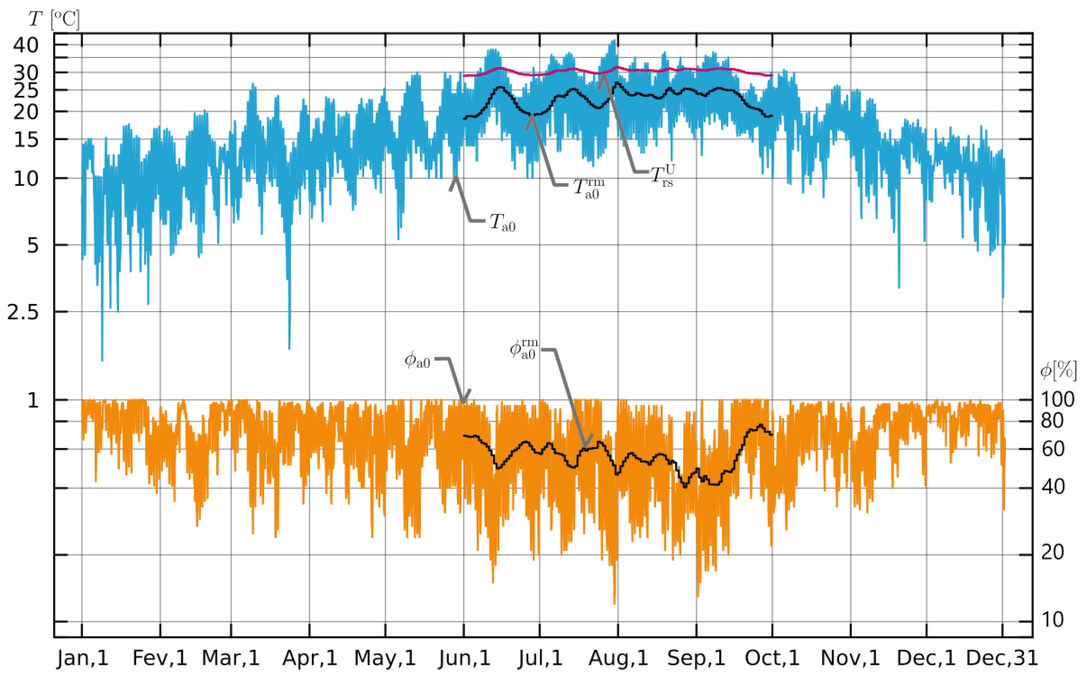
According to the adaptive comfort model from standard [71], during the cooling season, room setpoint has variable upper limits depending on the outdoor temperature. In this study, the climatic conditions considered are those of the TMY2 weather format file for the city of Beja [72], the district capital closest to the location of the EAHE under study. Figure 8 shows the temperature and relative humidity values from the TMY2 file (note the use of logarithmic scales on the left vertical axis for temperature $T[°\mathrm{C}]$ and on the right vertical axis for relative humidity $\varphi [\%]$).

As occurs in climatic regions of the Csa or BSk variety [73], summers in Beja are hot (with maximum temperatures reaching 40 °C) and dry (the median relative humidity between June and September is only 54%), with high daily thermal amplitudes. Winters, although mild, sometimes record temperatures close to zero. The high daily and annual thermal amplitudes observed in Figure 8 are beneficial for the operation of the EAHE in standalone cooling mode.

Figure 8 includes black lines representing the running mean (as defined in [71]) of temperature and relative humidity, $T_{\mathrm{a}0}^{\mathrm{rm}}$ and ${\varphi }_{\mathrm{a}0}^{\mathrm{rm}}$, respectively. Values of the running mean outdoor temperature above 20 °C are observed between June and September, and, for the purpose of assessing the potential for removing thermal loads in the EAHE, this period is considered the cooling season. As shown in Figure 8, between June and September, the values of the running mean relative humidity range between 40% and ∼70%.

Considering the values of the running mean outdoor temperature during the cooling season and the adaptive comfort model of standard [71], the maximum indoor setpoint value, $T_{\mathrm{rs}}^{\mathrm{U}}$, varies between 29 and 31 °C. The red line at the top of Figure 8 represents the evolution of this setpoint between June and September.

Knowing the temperature setpoint values that are appropriate for the outdoor temperature conditions, it is possible to apply Equation (32) and compare the cooling capacity of EAHEs operating in standalone and precooling modes.

3.2. Load Removal Sensitivity Analysis

The sensitivity analysis considers the EAHE and the reference parameters described in Section 2.4, Table 1, which correspond to the case used in the validation of the numerical model developed in this article. The reference climatic data used in the numerical simulations are those from the TMY2 file of Beja (see Figure 8). Since the operation of the EAHE for cooling is analyzed, only the data from this file between June and September are considered. For these months, and for the purposes of applying Equation (32), the temperature setpoint, $T_{\mathrm{rs}}^{\mathrm{U}}$, in the spaces to be cooled (with the EAHE operating in standalone cooling mode) is assumed to be equal to 29 °C.

Table 4. Parameters varied in the sensitivity analysis. Reference values, minima and maxima.

Parameter	Minimum	Reference	Maximum
$\dot{V}$ [m3/h]	1000	4000	8000
L [m]	18.75	70	140
$r_0$ [m]	0.30	0.5	1
$\alpha$ [m2/s]	$3\times {10}^{-7}$	$1\times {10}^{-6}$	$2\times {10}^{-6}$
$Z_0$ [m]	1.0	5.5	8.0
$\overline{\varphi }$ [%]	34% (1)	54% (2)	92% (3)

(1) Median determined after a constant was subtracted from the hourly values (June to September) of relative humidity from Beja’s TMY2 weather file whilst ensuring minimum values were larger than 0%; (2) median value obtained from Beja’s TMY2 weather file using data from June to September; (3) median determined after a constant was added to the hourly values (June to September) of relative humidity from Beja’s TMY2 weather file whilst ensuring maximum values never exceeded 100%.

presents the parameters that are varied in the sensitivity analysis, specifying the minimum and maximum limits considered, typically between approximately 1/4 and 2 times the reference value.

3.2.1. Case 1: Removal of Sensible Loads

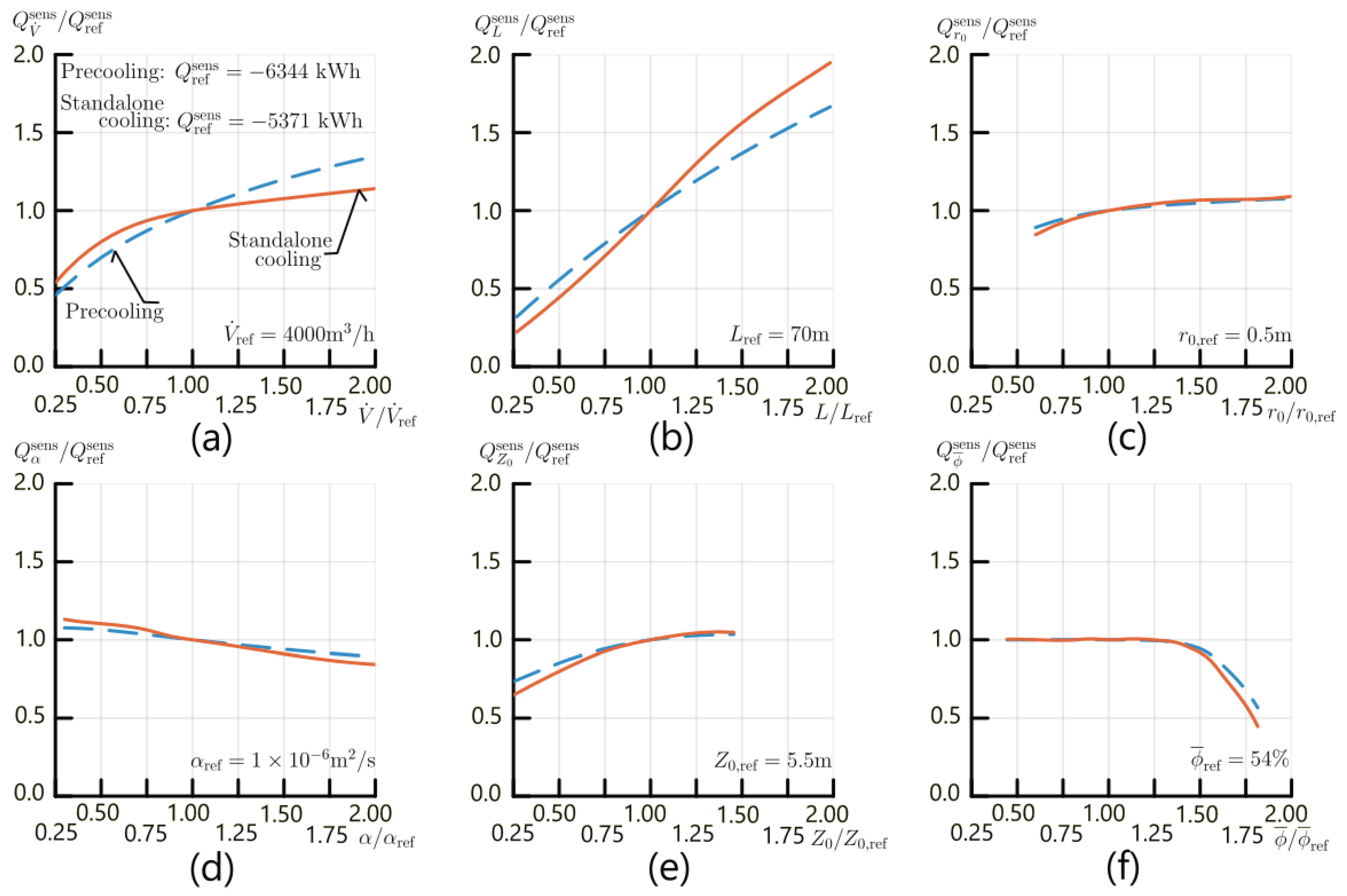
Figure 9 presents six graphs that facilitate the discussion of the sensitivity of sensible thermal load removal in the EAHE considering the independent variation of each of the parameters identified in Table 4.

On the abscissa axes, the ratios $x/x_{\mathrm{ref}}$ are presented, with $x\in \{\dot{V},L,r_0,\alpha ,Z_0,\overline{\varphi }\}$ being the parameter under analysis, varying between the minimum and maximum indicated in Table 4. Each graph identifies the reference value of the parameter under analysis, for example, $(x_{\mathrm{ref}}=){\dot{V}}_{\mathrm{ref}}=4000$ m³/h for graph (a), corresponding to the volumetric flow rate, and $(x\mathrm{ref}=)L_{\mathrm{ref}}=70$ m for graph (b), corresponding to the EAHE length. Abscissa values equal to 1 correspond to the cases $x=x_{\mathrm{ref}}$.

On the ordinate axes, the ratios $Q_x^{\mathrm{sens}}/Q_{\mathrm{ref}}^{\mathrm{sens}}$ are presented, where $Q_x^{\mathrm{sens}}$ is the sensible thermal load removed in the EAHE when parameter x is varied and $Q_{\mathrm{ref}}^{\mathrm{sens}}$ is the sensible thermal load removed in the EAHE under reference conditions. Since for $x/x_{\mathrm{ref}}=1$ the sensible thermal load removed in the EAHE is the reference value, it is observed in all six graphs that, at the abscissa, $x/x_{\mathrm{ref}}=1$ corresponds to the ordinate $Q_x^{\mathrm{sens}}/Q_{\mathrm{ref}}^{\mathrm{sens}}=1$.

In Figure 9a, values of the reference sensible thermal load are included when the EAHE operates in precooling mode, −6344 kWh, and in standalone cooling mode, −5371 kWh. The results of the ratio $Q_x^{\mathrm{sens}}/Q_{\mathrm{ref}}^{\mathrm{sens}}$ for these two EAHE operating modes are represented by blue dashed lines for precooling and by orange solid lines for standalone cooling.

A preliminary analysis of the values of sensible thermal load $Q_{\mathrm{ref}}^{\mathrm{sens}}$ removed under reference conditions confirms the cooling potential of the EAHE. Using the values presented in Figure 9a and considering a cooled floor area of 450 m² for the office building, it is possible, during the cooling season from June to September, to remove 12 to 14 kWh/m² of sensible heat (for standalone and precooling modes, respectively), values close to those accepted for low-energy buildings implementing appropriate energy conservation practices [74,75].

As expected, the value $Q_{\mathrm{ref}}^{\mathrm{sens}}$ obtained with the EAHE operating in standalone cooling mode, −5371 kWh, is lower (in absolute value) than that for precooling operation. Indeed, under very high outdoor temperatures, periods are observed in which the outlet temperature of the EAHE is higher than the room setpoint; i.e., $T_{\mathrm{aL}}>T_{\mathrm{rs}}^{\mathrm{U}}=29°\mathrm{C}$. As explained in Section 3.1, with regard to Figure 7, during these periods, an EAHE operating in standalone cooling mode ceases to remove thermal load from the spaces, whereas one operating in precooling mode does not.

Analyzing, across the six graphs, the increase in the ratio $Q_x^{\mathrm{sens}}/Q_{\mathrm{ref}}^{\mathrm{sens}}$ due to variations in $x/x_{\mathrm{ref}}$, it is concluded that increasing the length L of the EAHE produces the greatest effect, a result also obtained by [32,34,36,76]. By doubling the reference length of the EAHE, the energy transferred in precooling mode increases by approximately 60% and in standalone cooling mode by approximately 100%. It should be noted that the difference between these percentages does not mean that the standalone cooling mode removes more heat from the outdoor air than the precooling mode; it merely reflects the fact that, for longer lengths L, since the air leaving the EAHE is at a temperature below the room setpoint, the condition $T_{\mathrm{aL}}<T_{\mathrm{rs}}^{\mathrm{U}}$ in Equation (32) is eliminated, yielding $Q_{\mathrm{StandaloneCool}}^{\mathrm{sens}}=Q_{\mathrm{Preecool}}^{\mathrm{sens}}$.

The second most notable effect on the increase in the thermal load removed by the EAHE is achieved by increasing the volumetric flow rate, $\dot{V}$, which is also in agreement with [15,77]. By doubling the reference flow rate from 4000 to 8000 m³/h, the energy removed by the EAHE operating in precooling mode increases by approximately 40%. This increase is much smaller when the EAHE operates in standalone cooling mode, being less than 20%. Indeed, increasing the volumetric flow rate, i.e., increasing airflow velocity, reduces the air residence time inside the EAHE, thereby decreasing the temperature change in the air between the inlet and outlet [35,37,38,39]. Because, in standalone cooling mode, the cooling capacity of the rooms is limited by a maximum outlet air temperature equal to the room setpoint, there is a maximum allowable flow rate in standalone cooling mode [38,78].

Regarding the EAHE’s radius, the soil thermal diffusivity, the depth at which the EAHE is buried, and the median outdoor air relative humidity, changes in these parameters have a smaller effect on the sensible load removed by the EAHE. Indeed, for depths larger than 3.5 m ($0.625Z_{0,\mathrm{ref}}$), variations in the sensible load ratio become negligible. For the median outdoor air relative humidity, the sensible load ratio does not change up to 1.375${\overline{\varphi }}_{\mathrm{ref}}$, i.e., up to 75% relative humidity; however, above this value, a significant and abrupt decrease in the sensible thermal load removed by the EAHE is observed. This abrupt reduction is explained by the sudden increase in latent heat transfer occurring at the inner surface of the EAHE.

In the following subsection, the removal of latent thermal loads is addressed in greater detail.

3.2.2. Case 2: Removal of Latent Loads

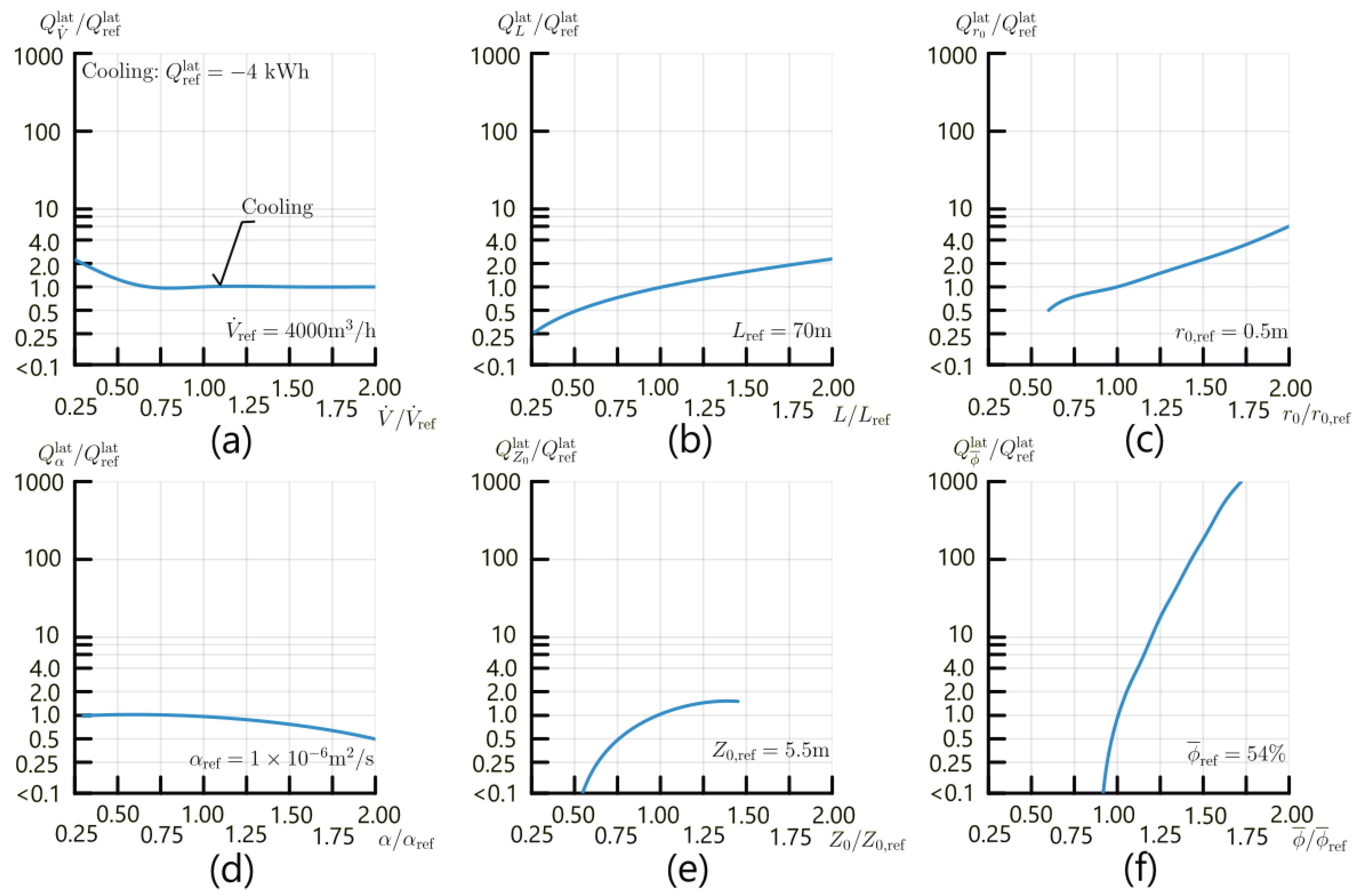
To understand how latent load removal in the EAHE is affected by variations in the parameters included in Table 4, Figure 10 presents the ratios of latent loads, $Q_x^{\mathrm{lat}}/Q_{\mathrm{ref}}^{\mathrm{lat}}$ with $x\in \{\dot{V},L,r_0,\alpha ,Z_0,\overline{\varphi }\}$, determined during the cooling season, between June and September. Figure 10 is analogous to Figure 9 except for the representation of latent load ratios without the distinction between EAHE operating modes and the use of the logarithmic scale in the ordinate axes.

From Figure 10a, the very low value of latent thermal load removed by the EAHE under reference conditions immediately stands out: −4 kWh, less than 0.1% of the sensible thermal loads removed over the same period. This result is consistent with that reported in Section 2.6 based on monitoring data obtained near Beja, where it was not possible to conclude significant differences between the humidity ratio of the air at the inlet and outlet of an EAHE equal to the reference one. As noted in Section 2.6, this low removal of latent thermal loads is due to the hot and dry summer climate conditions.

The adoption of the logarithmic scale exaggerates the small variations in the latent load removed by the EAHE. Still, the details provided in Figure 10 provide additional insight into the effect of the parameters being studied.

Analyzing, for Figure 10a–c, the increase in the ratio $Q_x^{\mathrm{lat}}/Q_{\mathrm{ref}}^{\mathrm{lat}}$ due to variations in $x/x_{\mathrm{ref}}$, it is concluded that latent load removal increases when variations in the parameters under analysis lead to lower outlet air temperatures of the EAHE; i.e., with lower flow rates, $\dot{V}$ (per pipe), greater lengths, L, and larger radii, $r_0$ (keeping the flow rate constant, this implies a longer air residence time in the EAHE), conditions that simultaneously enhance standalone cooling [39]. Increasing the depth at which the EAHE is buried increases latent heat exchange; see Figure 10e. However, since the reference depth $Z_{0,\mathrm{ref}}=$ 5.5 m is already large, no significant increases are observed for greater burial depths. Regarding soil thermal diffusivity, $\alpha$, the effect of this parameter is negligible.

The increases in the ratio $Q_x^{\mathrm{lat}}/Q_{\mathrm{ref}}^{\mathrm{lat}}$ for the parameters discussed so far never exceed a factor of 10; that is, they represent a modest increase from 4 kWh to less than 40 kWh of latent thermal load removed in the EAHE. The only significant increase in latent heat exchange is that observed in Figure 10f, which describes the effect of variations in the median outdoor air relative humidity. Indeed, assuming an increase in the median outdoor relative humidity of about 50% relative to the reference value, from 54 to 80%, the latent load removed by the EAHE increases by ∼150 times, i.e., by approximately 600 kWh. This increase is accompanied by an equivalent reduction in the sensible load removed, as confirmed in Figure 9f: note the ordered pair $\left(\overline{\varphi }/{\overline{\varphi }}_{\mathrm{ref}},Q_{\overline{\varphi }}^{\mathrm{sens}}/Q_{\mathrm{ref}}^{\mathrm{sens}}\right)=(1.5,0.9)$, which reflects a reduction in sensible thermal load of approximately 600 kWh. The experimental studies reported by [17,18] also demonstrate the importance of accounting for latent heat transfer when modeling EAHEs operating in humid climates.

3.3. Discussion of the Load Removal Sensitivity Analysis

A first aspect worth highlighting in this discussion is that the operation of the EAHE under reference conditions is capable of removing a sensible thermal load during the cooling season on the order of 12∼14 kWh/m², a value close to that observed in low-energy buildings implementing good energy conservation practices (adequate thermal insulation and shading, among others [74,75]). As shown in Section 3.2, by increasing the length L and the flow rate $\dot{V}$, it is possible to further increase (by a factor greater than 1.5) EAHE cooling capacity. Simultaneously, the removal of sensible thermal load from the air supplied to the rooms can be augmented, complementing the use of the EAHE with passive building cooling techniques, namely nighttime cooling and the use of the building’s thermal mass [28,29,30,31,64]. Combining these strategies, room load removal can be increased up to values close to 20 kWh/m², a mark supporting the use of EAHEs (replacing conventional air conditioning) for standalone cooling in office buildings.

Another aspect worth emphasizing is the need, in standalone cooling mode, for the EAHE design choices to ensure that the outlet air temperature of the EAHE does not exceed the temperature setpoint in the rooms to be cooled. Although this requirement may appear obvious, it highlights a fundamental aspect in EAHE design: deciding whether priority should be given, in thermal load removal, to higher flow rates with smaller reductions in air temperature (as stated in numerous studies [9,19,34,46]) or, on the contrary, if the decrease in air temperature within the EAHE should be promoted by reducing the flow rates.

In precooling operating mode, thermal load removal in the EAHE can be achieved in both ways. If priority is given to high flow rates, smaller reductions in air temperature occur between the inlet and outlet of the EAHE; however, because there is a refrigeration unit downstream of the EAHE, the supply of air to the rooms at a temperature below the setpoint is ensured by the refrigeration system.

Without mechanical means for reducing air temperature, in the standalone cooling operating mode of the EAHE, there exists a flow rate above which, due to the smaller temperature drop between the inlet and outlet of the EAHE, the outlet air temperature exceeds the room setpoint. For this flow rate (and higher ones), the cooling function of the office room ceases. It is therefore concluded that, in the design of EAHE systems intended to operate in standalone cooling mode, priority should be given to reducing the temperature of the air flowing through the EAHE, while flow rate requirements may be adjusted through geometry (radius and number of pipes).

As seen from the results of the sensitivity analysis, in practice, the enhancement of temperature reduction and the enhancement of the removal of sensible cooling loads are achieved through:

• An EAHE of greater length;
• An EAHE buried at greater depth but only up to the limit at which disturbances caused by the climate cease to be significant ($Z_0⪆3$ m [37,57,79]);
• For a given pipe length and flow rate, an EAHE with a larger radius (lowering airflow velocity and increasing air residence time within the ground).

In addition to these conclusions of a geometric nature and related to the installation (depth) of the EAHE, the results of the sensitivity analysis also made it possible to conclude:

• The low sensitivity of the cooling loads removed by the EAHE to: (i) variations in soil thermal diffusivity; (ii) the depth at which the EAHE is buried given $Z_0⪆3$ m; and (iii) (for dry climates) latent heat exchanges.

This last conclusion is particularly relevant as it justifies the use of the developed computational model at the design stage despite uncertainties in soil properties, in the installation depth (provided it remains below a given threshold), and for locations with dry climates despite the lack of quantitative validation of the phase-change model. This conclusion also explains why simplified models, including steady-state and graphical approaches, have been successfully employed by other authors to analyze the thermal behavior of EAHEs [34,38,48,55].

On the other hand, for humid climates, the results highlight the fundamental importance of correctly modeling latent heat exchanges. Indeed, since the conditions that favor EAHE operation in standalone cooling mode are the same as those that contribute to the occurrence of condensation in humid climates, this reinforces the importance not only of modeling but also validating the phase-change model. As shown, the increase in condensation leads to a reduction in the sensible thermal load removed, and condensation can compromise the quality of the air supplied to the rooms (through the entrainment of fungal spores and bacteria that develop on wet surfaces [9,19]), something that should be anticipated and prevented at the design stage.

4. Conclusions

In this article, a numerical model was developed using a free and open-access scientific programming language to describe the thermo-hygrometric behavior of EAHE systems used for space cooling. The application of the numerical model led to the conclusion that EAHEs can realistically operate in standalone cooling mode, removing up to 20 kWh/m² of sensible load, thus making the use of mechanical cooling systems unnecessary and, consequently, contributing to more ecological office cooling solutions. Additionally, it is concluded that, in the design of EAHEs operating in standalone cooling mode, high airflow velocities should be avoided; instead, designs should promote lower outlet air temperatures.

In practice, projects of EAHEs for standalone cooling should prioritize:

• Geometries with greater length;
• Burial depths that allow taking advantage of the seasonal phase shift of ground temperature (more than 3 m);
• Lower airflow velocities (favoring the air residence time within the ground), which can be achieved through larger EAHE radii (or by distributing the flow across multiple pipes, as in the case studied in this article, which uses two pipes with 0.5 m radius).

Moreover:

• High precision in defining soil properties or in determining the burial depth of the EAHE is not required (provided it is below a given threshold depth);
• For dry climates, moisture mass transfer phenomena have a negligible effect on EAHE performance;
• For humid climates (with median relative humidity values during the cooling season of 75% or higher), due to the prevalence of condensation on the inner surface of the EAHE, the use of an EAHE operating in standalone cooling mode is not recommended.

Based on the successful validation of the numerical model against monitoring data in a region with hot and dry summers, both the investment analysis and the design of large-diameter EAHEs—operating in standalone cooling or precooling mode—can be carried out using free and open-source scientific programming languages. As demonstrated, these languages enable high-level symbolic representations, namely the definition of the problem using the syntax of the mathematical formulation, and provide access to tools that automatically generate meshes, perform the necessary discretization, and obtain the numerical solutions of complex problems. These languages therefore represent an alternative to commercial tools, making EAHE analysis and design accessible to a larger number of engineers and researchers and, in this way, paving the way for reducing reliance on mechanical refrigeration for office cooling, with resulting environmental benefits.

Limitations and Future Work

Although the computational model achieves a good fit to the analytical solutions considered, experimental and quantitative validation of the condensate mass based on monitoring data obtained in a humid climate is still lacking.

As the results of this article show, humid climates are not favorable for EAHE operation in standalone cooling mode. However, if one intends to study precooling operation or the use of EAHEs for latent heat load removal, it is important to validate the latent heat exchange model used in this study. Indeed, according to [80], the fit of the mass transfer model depends on the selection of either saturated or unsaturated condensation models and, naturally, on the validated coefficients used in Equation (1). Thus, a relevant research topic consists of using monitoring data obtained in humid climates for the validation of latent heat transfer in large-diameter EAHEs.

Additional relevant research topics include: (i) expanding the sensitivity analysis to present results that consider the combined effect of multiple parameters; (ii) coupling the developed model with building energy simulation models; and (iii) taking into account future climatic uncertainties, which point toward elevated annual air temperatures and more frequent weather anomalies, with a consequent increase in cooling demand. Given the critical need to guarantee cooling during catastrophic events involving power grid disruptions, continuing to design and develop alternatives to mechanical air conditioning systems, such as an EAHE operating in standalone cooling mode, emerges as highly relevant.