Active and Backstepping Control for Stabilization and Synchronization of a Four-Dimensional Hyperchaotic Finance System

Abstract

This paper addresses the stabilization and drive–response synchronization of the four-dimensional hyperchaotic finance model using active backstepping (ABS) and active control (AC). The contribution is not the introduction of a new control paradigm but a unified implementation of AC and ABS for the Yu finance model, together with explicit Lyapunov convergence estimates, reproducible numerical benchmarking, and robustness-oriented performance assessment. For the ideal full-state-feedback setting, Lyapunov arguments establish exponential stabilization for the ABS-controlled system and exponential synchronization for both AC and ABS. The numerical protocol quantifies settling time, norm-relative overshoot, envelope-based decay rate, integrated control energy, CPU time, and actuator peak/RMS values. The results show that AC provides smooth and energy-efficient synchronization, whereas ABS gives fast convergence and a nonlinear Lyapunov-based stabilization framework but requires higher actuation effort. Robustness tests under parameter mismatch and additive measurement noise indicate bounded trajectories and decaying synchronization errors under the tested perturbation levels. The results also clarify the trade-off between convergence speed, control energy, implementation complexity, and actuator feasibility.

1. Introduction

Chaotic dynamics—deterministic yet highly sensitive to initial conditions—arise naturally in nonlinear models across physics, biology, engineering, telecommunications, and economics. In financial systems, such behavior can jeopardize stability and frustrate long-run forecasting, motivating feedback designs that either stabilize trajectories or synchronize coupled models.

In economic modeling, both chaos and hyperchaos have been reported. In this study, hyperchaos refers to the presence of at least two positive Lyapunov exponents, indicating richer instability and lower predictability than standard chaos. Early demonstrations of endogenous instability in macroeconomic settings include Grandmont [1]. A compact 3-D finance model capturing the interaction among interest rate, investment demand, and price index was proposed by Jun-hai and Yu-Shu [2]. Yu et al. [3] extended the three-dimensional finance model to a four-dimensional hyperchaotic finance system by introducing an additional state variable representing the average profit margin:

$$\begin{array}{cc}\hfill \dot{x}& =z+(y-a)x+w,\hfill \\ \hfill \dot{y}& =1-by-x^2,\hfill \\ \hfill \dot{z}& =-x-cz,\hfill \\ \hfill \dot{w}& =-dxy-kw.\hfill \end{array}$$

(1)

Here, $x,y,z$, and w denote the interest rate, investment demand, price index, and average profit margin, respectively. The positive parameters $a,b,c,d$, and k and their economic interpretations are summarized in

Table 1. State variables and parameters for the Yu 4-D finance model (1).

Symbol	Meaning
x	Interest rate
y	Investment demand
z	Price index
w	Average profit margin
a	Saving amount/saving propensity parameter
b	Cost per investment
c	Price-index adjustment (damping) rate
d	Coupling strength in profit-margin dynamics
k	Profit-margin decay (mean-reversion) rate

.

Recent studies also show that high-dimensional chaotic and hyperchaotic dynamics have uses beyond stabilization problems, including image processing, secure communication, and image encryption. For example, fractional-order variational models and comprehensive image-encryption surveys emphasize the value of nonlinear and fractional-order dynamics in modern computational imaging and security applications [4,5]. This broader context motivates careful benchmarking of hyperchaotic finance controllers since similar high-dimensional instability mechanisms may be exploited or suppressed depending on the application.

Motivation and Research Gap

For the 4-D model (1), the reported controllers include linear and speed-feedback stabilization [3], recursive backstepping and backstepping–sliding-mode variants [6], chatter-reduced SMC [7], adaptive/robust schemes with parameter estimation [8,9], and single-controller approaches based on Routh–Hurwitz stability criteria [10]. The broader foundations are provided by classical work on chaos control and drive–response synchronization [11,12], while comparisons between active-control and backstepping strategies have been reported for related chaotic systems [13].

Despite substantial progress, several limitations remain in the literature on the Yu four-dimensional finance system. The existing designs include linear feedback, speed-feedback stabilization, recursive backstepping, sliding-mode variants, chatter-reduced sliding-mode control, adaptive/robust schemes, and single-controller approaches [3,6,7,8,9,10]. Therefore, the novelty claimed in the present paper is deliberately limited and specific: we do not claim to introduce active control or backstepping as new methods. Instead, the contribution is a unified AC–ABS implementation for the Yu model, an explicit convergence-rate statement for the ABS construction, a common stabilization–synchronization benchmark, and a direct discussion of control energy, actuator magnitude, and robustness under parameter mismatch and noise.

A further limitation of earlier comparisons is that stabilization and synchronization are often studied separately. Performance indicators such as settling time, norm-relative overshoot, exponential decay rate, integrated control energy, actuator peak/RMS values, and computational cost are not always reported together. This makes it difficult to judge whether a controller is fast because it is genuinely efficient or because it uses substantially larger control amplitudes. In addition, robustness tests under simultaneous parameter mismatch and measurement noise are rarely reported in a reproducible form. The present work addresses these gaps by using a common numerical protocol and by interpreting the observed trade-offs rather than presenting a single controller as uniformly superior.

We propose an active-control synchronizer and an active-backstepping framework for the stabilization and drive–response synchronization of the four-dimensional finance system. Within a Lyapunov framework, we prove exponential convergence of the controlled error dynamics and derive an explicit convergence-rate estimate for ABS in the ideal full-state-feedback setting. Using a common reproducible benchmark with identical solver settings, initial conditions, and tolerances, we compare the proposed methods with a classical speed-feedback baseline and discuss their relation to more modern nonlinear-control approaches. Performance is reported using settling time, norm-relative overshoot, envelope-based decay rate, integrated control energy, actuator magnitudes, and CPU time. Robustness is examined numerically under parameter mismatch and additive measurement noise.

2. Theoretical Framework

This section presents the stability tools used in the analysis and derives the active-control, speed-feedback, and active-backstepping formulations used for the Yu four-dimensional finance model.

2.1. Preliminaries

2.1.1. Lyapunov (Direct) Method

Let $\dot{\mathit{x}}=f\left(\mathit{x}\right)$ with $f\left(\mathbf{0}\right)=\mathbf{0}$. If there exists $V\in C^1$ on a neighborhood $\mathcal{D}\subset {\mathbb{R}}^n$ of the origin such that $V\left(\mathit{x}\right)>0$ for $\mathit{x}\ne \mathbf{0}$, $V\left(\mathbf{0}\right)=0$, and $\dot{V}\left(\mathit{x}\right)\le 0$ on $\mathcal{D}$, then the origin is (Lyapunov) stable. If $\dot{V}\left(\mathit{x}\right)<0$ on $\mathcal{D}\setminus \left\{\mathbf{0}\right\}$, the origin is (locally) asymptotically stable. If there exist $c_1,c_2,c_3>0$ with

$$c_1{\parallel \mathit{x}\parallel }_2^2\le V\left(\mathit{x}\right)\le c_2{\parallel \mathit{x}\parallel }_2^2,\dot{V}\left(\mathit{x}\right)\le -c_3{\parallel \mathit{x}\parallel }_2^2,$$

then the origin is (locally) exponentially stable and ${\parallel \mathit{x}\left(t\right)\parallel }_2\le \sqrt{\frac{c_2}{c_1}}{e}^{-{\displaystyle \frac{c_3}{2c_2}}t}{\parallel \mathit{x}\left(0\right)\parallel }_2$. For instability, a Chetaev condition applies: if there exists $V\in C^1$ with $V\left(\mathbf{0}\right)=0$ and $V\left(\mathit{x}\right)>0$, $\dot{V}\left(\mathit{x}\right)>0$ on a punctured neighborhood, then the origin is unstable.

2.1.2. Routh–Hurwitz Criterion

Let $p\left(\lambda \right)={\lambda }^n+a_1{\lambda }^{n-1}+\cdots +a_n$ with real coefficients and $a_0:=1$ (monic). Form the $n\times n$ Hurwitz matrix $H=\left(h_{ij}\right)$ with $h_{ij}=a_{2i-j}$ using the conventions $a_0=1$ and $a_k=0$ for $k<0$ or $k>n$. Denote by ${\Delta }_k=det{H}_k$ the kth leading principal minor. Then p is Hurwitz (all zeros in the open left half–plane) iff ${\Delta }_k>0$ for $k=1,\dots ,n$.

2.1.3. Linearization (Indirect Method)

Let ${\mathit{x}}^{\star }$ be an equilibrium of $\dot{\mathit{x}}=f\left(\mathit{x}\right)$, and let $J={\displaystyle \frac{\partial f}{\partial \mathit{x}}}{|}_{{\mathit{x}}^{\star }}$. If all eigenvalues of J have strictly negative real parts, then ${\mathit{x}}^{\star }$ is (locally) exponentially stable; if at least one has positive real part, it is unstable; if some have zero real part and none is positive, linearization is inconclusive.

2.2. Control Methods

2.2.1. Active Control (Generic Drive–Response)

Consider the drive (master) system

$$\dot{\mathit{\xi }}=M\mathit{\xi }+g\left(\mathit{\xi }\right),\mathit{\xi }\in {\mathbb{R}}^n,$$

(2)

with constant $M\in {\mathbb{R}}^{n\times n}$ and locally Lipschitz $g:{\mathbb{R}}^n\to {\mathbb{R}}^n$. The response (slave) is

$$\dot{\mathit{\eta }}=M\eta +g\left(\mathit{\eta }\right)+\mathit{u},\mathit{\eta }\in {\mathbb{R}}^n.$$

(3)

With error $\mathit{e}:=\mathit{\eta }-\mathit{\xi }$,

$$\dot{\mathit{e}}=M\mathit{e}+\left(g\left(\mathit{\eta }\right)-g\left(\mathit{\xi }\right)\right)+\mathit{u}=:M\mathit{e}+\mathit{G}(\mathit{\xi },\eta )+\mathit{u}.$$

The active control law

$$\mathit{u}=-\mathit{G}(\mathit{\xi },\mathit{\eta })+K\mathit{e}$$

(4)

gives $\dot{\mathit{e}}=(M+K)\mathit{e}$. If $M+K$ is Hurwitz, then ${\parallel \mathit{e}\left(t\right)\parallel }_2\le C{e}^{-\alpha t}{\parallel \mathit{e}\left(0\right)\parallel }_2$ for suitable $C,\alpha >0$ (via a quadratic Lyapunov function).

Instantiation for the Finance Model

For the Yu system, the synchronization error dynamics contain state-dependent terms through $x_1+x_2$. We therefore choose the state-dependent gain $K(x_1,x_2)=A-M(x_1,x_2)$ with $A=-I_4$ so that the closed-loop error system reduces to $\dot{\mathit{e}}=A\mathit{e}=-\mathit{e}$, yielding global exponential synchronization.

Proposition 1

(Exponential synchronization under active control). Let the drive–response pair be given by (2) and (3) instantiated for the Yu model, and apply the active-control law (14) with $A=-I_4$; i.e., use the components in (16). Then the synchronization error $\mathit{e}=(x_2-x_1,y_2-y_1,z_2-z_1,w_2-w_1)$ satisfies

$${\parallel \mathit{e}\left(t\right)\parallel }_2\le e^{-t}{\parallel \mathit{e}\left(0\right)\parallel }_2,t\ge 0,$$

so synchronization is global and exponential with decay rate 1. Moreover, each control component is a static polynomial function of the measured states; hence the feedback law is globally defined and locally Lipschitz, with no singularities.

Proof. 

By construction, substituting (14) into the error system (13) gives the linear closed-loop dynamics (15): $\dot{\mathit{e}}=A\mathit{e}=-\mathit{e}$. The solution is $\mathit{e}\left(t\right)=e^{-t}\mathit{e}\left(0\right)$, implying the stated bound with rate 1. From (16), each $u_i$ is a polynomial in the measured states $(x_1,y_1,z_1,w_1,x_2,y_2,z_2,w_2)$. Thus, the controller is globally defined and locally Lipschitz.    □

2.2.2. ABS for the Yu Model (Global Stabilization)

For the controlled model

$$\begin{array}{cc}\hfill \dot{x}& =z+(y-a)x+w+u_1,\hfill \\ \hfill \dot{y}& =1-by-x^2+u_2,\hfill \\ \hfill \dot{z}& =-x-cz+u_3,\hfill \\ \hfill \dot{w}& =-dxy-kw+u_4,\hfill \end{array}$$

(5)

apply the static prefeedback

$$\begin{array}{cc}\hfill u_1& =-z-(y-a)x-w+y,\hfill \\ \hfill u_2& =-1+by+x^2+z,\hfill \\ \hfill u_3& =x+cz+w,\hfill \\ \hfill u_4& =dxy+kw+v,\hfill \end{array}$$

(6)

to obtain the integrator chain

$$\dot{x}=y,\dot{y}=z,\dot{z}=w,\dot{w}=v.$$

(7)

Let

$${\phi }_1=x,{\phi }_2=x+y,{\phi }_3=2x+2y+z,{\phi }_4=3x+5y+3z+w,$$

and $V=\frac{1}{2}{\sum }_{i=1}^4{\phi }_i^2$. Along (7),

$$\dot{V}=-{\phi }_1^2-{\phi }_2^2-{\phi }_3^2-{\phi }_4^2+{\phi }_4\left(5x+10y+9z+4w+v\right).$$

Choose

$$v=-\left(5x+10y+9z+4w\right)-C{\phi }_4,C>0,$$

(8)

to get

$$\dot{V}=-{\phi }_1^2-{\phi }_2^2-{\phi }_3^2-(1+C){\phi }_4^2\le -({\phi }_1^2+{\phi }_2^2+{\phi }_3^2+{\phi }_4^2)=-2V,$$

hence $V\left(t\right)\le V\left(0\right)e^{-2t}$ and ${\parallel \phi \left(t\right)\parallel }_2\le e^{-t}{\parallel \phi \left(0\right)\parallel }_2$. Because $\phi =T{\left[xyzw\right]}^{\top }$ with T lower-triangular and nonsingular, ${\parallel \left[xyzw\right]}^{\top }{\parallel }_2\le \kappa e^{-t}{\parallel {\left[x\left(0\right)y\left(0\right)z\left(0\right)w\left(0\right)\right]}^{\top }\parallel }_2$ for some $\kappa >0$. Substituting (8) into (6) yields the implementable ABS stabilizer

$$\begin{array}{cc}\hfill u_1& =-z-(y-a)x-w+y,\hfill \\ \hfill u_2& =-1+by+x^2+z,\hfill \\ \hfill u_3& =x+cz+w,\hfill \\ \hfill u_4& =dxy+kw-\left(5x+10y+9z+4w\right)-C(3x+5y+3z+w).\hfill \end{array}$$

(9)

2.2.3. ABS for the Yu Model (Drive–Response Synchronization)

For the drive $(x_1,y_1,z_1,w_1)$ and response $(x_2,y_2,z_2,w_2)$, define $\mathit{e}={(e_1,e_2,e_3,e_4)}^T={(x_2-x_1,y_2-y_1,z_2-z_1,w_2-w_1)}^T$. With the static (polynomial) prefeedback

$$\begin{array}{cc}\hfill u_1& =a{e}_1+e_2-e_3-e_4-(y_2{x}_2-y_1{x}_1),\hfill \\ \hfill u_2& =b{e}_2+(x_1+x_2)e_1+e_3,\hfill \\ \hfill u_3& =e_1+c{e}_3+e_4,\hfill \\ \hfill u_4& =-d{y}_1{x}_1+d{y}_2{x}_2+k{e}_4+v,\hfill \end{array}$$

(10)

the error dynamics are the chain

$${\dot{e}}_1=e_2,{\dot{e}}_2=e_3,{\dot{e}}_3=e_4,{\dot{e}}_4=v.$$

Using

$${\phi }_1=e_1,{\phi }_2=e_1+e_2,{\phi }_3=2e_1+2e_2+e_3,{\phi }_4=3e_1+5e_2+3e_3+e_4,$$

and $V=\frac{1}{2}{\sum }_{i=1}^4{\phi }_i^2$, the choice

$$v=-5e_1-10e_2-9e_3-4e_4-C{\phi }_4,C>0,$$

(11)

gives $\dot{V}\le -2V$. Since the transformation from e to $\varphi$ is linear and nonsingular, there exists $\kappa >0$ such that ${\parallel e\left(t\right)\parallel }_2\le \kappa e^{-t}{\parallel e\left(0\right)\parallel }_2$. The implementable synchronizer is

$$\begin{array}{cc}\hfill u_1& =a{e}_1+e_2-e_3-e_4-y_2{x}_2+y_1{x}_1,\hfill \\ \hfill u_2& =b{e}_2+(x_1+x_2)e_1+e_3,\hfill \\ \hfill u_3& =e_1+c{e}_3+e_4,\hfill \\ \hfill u_4& =-d{y}_1{x}_1+d{y}_2{x}_2+k{e}_4-5e_1-10e_2-9e_3-4e_4-C(3e_1+5e_2+3e_3+e_4).\hfill \end{array}$$

(12)

2.2.4. Active Control for the Yu Model (State-Dependent Gain)

Subtracting the drive from the response gives the error model

$$\dot{\mathit{e}}=M(x_1,x_2)\mathit{e}+\mathit{G}(x_1,y_1,x_2,y_2)+\mathit{u},$$

(13)

with

$$M(x_1,x_2)=\left(\begin{array}{cccc}-a& 0& 1& 1\\ -(x_1+x_2)& -b& 0& 0\\ -1& 0& -c& 0\\ 0& 0& 0& -k\end{array}\right),\mathit{G}=\left(\begin{array}{c}{y}_2{x}_2-y_1{x}_1\\ 0\\ 0\\ d(y_1{x}_1-y_2{x}_2)\end{array}\right).$$

Choose

$$\mathit{u}=-\mathit{G}+K(x_1,x_2)\mathit{e},K(x_1,x_2)=A-M(x_1,x_2),A:=-I_4,$$

(14)

to obtain

$$\dot{\mathit{e}}=(M+K)\mathit{e}=A\mathit{e}=-\mathit{e},$$

(15)

and hence ${\parallel \mathit{e}\left(t\right)\parallel }_2\le e^{-t}{\parallel \mathit{e}\left(0\right)\parallel }_2$. Componentwise,

$$\begin{array}{cc}\hfill u_1& =(a-1)e_1-e_3-e_4-(y_2{x}_2-y_1{x}_1),\hfill \\ \hfill u_2& =(x_1+x_2)e_1+(b-1)e_2,\hfill \\ \hfill u_3& =e_1+(c-1)e_3,\hfill \\ \hfill u_4& =-d{y}_1{x}_1+d{y}_2{x}_2+(k-1)e_4.\hfill \end{array}$$

(16)

The controller is static and polynomial in the measured states because of the bilinear products; hence the feedback law is globally defined and locally Lipschitz.

2.2.5. Speed-Feedback for the Yu Model (Local Stabilization at $P_0$)

For comparison with the speed-feedback control method used by Yu et al. [3], we consider local stabilization of the equilibrium point

$$P_0=\left(0,{\displaystyle \frac{1}{b}},0,0\right).$$

Introducing the shifted variables

$$X=x,Y=y-{\displaystyle \frac{1}{b}},Z=z,W=w,$$

system (1) can be rewritten as

$$\begin{array}{cc}\hfill \dot{X}& =Z+\left(Y+{\displaystyle \frac{1}{b}}-a\right)X+W,\hfill \\ \hfill \dot{Y}& =-bY-X^2,\hfill \\ \hfill \dot{Z}& =-X-cZ,\hfill \\ \hfill \dot{W}& =-{\displaystyle \frac{d}{b}}X-dXY-kW.\hfill \end{array}$$

The speed-feedback controller is introduced in the W-equation as

$$\dot{W}=-{\displaystyle \frac{d}{b}}X-dXY-kW-K\dot{X},$$

where $K>0$ is the feedback gain. Therefore, the controlled shifted system becomes

$$\begin{array}{cc}\hfill \dot{X}& =Z+\left(Y+{\displaystyle \frac{1}{b}}-a\right)X+W,\hfill \\ \hfill \dot{Y}& =-bY-X^2,\hfill \\ \hfill \dot{Z}& =-X-cZ,\hfill \\ \hfill \dot{W}& =-{\displaystyle \frac{d}{b}}X-dXY-kW-K\left[Z+\left(Y+{\displaystyle \frac{1}{b}}-a\right)X+W\right].\hfill \end{array}$$

The Jacobian matrix of the controlled system at the shifted equilibrium $(X,Y,Z,W)=(0,0,0,0)$ is

$$J_{\mathrm{SFC}}=\left(\begin{array}{cccc}{\displaystyle \frac{1}{b}}-a& 0& 1& 1\\ 0& -b& 0& 0\\ -1& 0& -c& 0\\ -{\displaystyle \frac{d}{b}}-K\left({\displaystyle \frac{1}{b}}-a\right)& 0& -K& -(k+K)\end{array}\right).$$

The corresponding characteristic equation is

$$(\lambda +b)\left({\lambda }^3+n_1{\lambda }^2+n_2\lambda +n_3\right)=0,$$

where

$$\begin{array}{cc}\hfill n_1& =K+a+c+k-{\displaystyle \frac{1}{b}},\hfill \\ \hfill n_2& =c(a+K)+k(a+c)+1+{\displaystyle \frac{d-k-c}{b}},\hfill \\ \hfill n_3& =k\left(ac+1-{\displaystyle \frac{c}{b}}\right)+{\displaystyle \frac{cd}{b}}.\hfill \end{array}$$

By the Routh–Hurwitz criterion, the cubic factor is Hurwitz if

$$n_1>0,n_2>0,n_3>0,n_1{n}_2>n_3.$$

For the nominal parameter values

$$(a,b,c,d,k)=(0.9,0.2,1.5,0.2,0.17),$$

these inequalities give $K>3.46$. Hence, choosing $K=3.5$ gives the linearized eigenvalues

$$-0.2000,-1.0233,-0.0233\pm 0.7808i.$$

Therefore, the equilibrium $P_0$ is locally asymptotically stable under the speed-feedback controller. This controller is used here only as a local stabilization baseline for comparison with the proposed active-backstepping controller.

The two stabilization targets have different interpretations. In the original economic coordinates, $P_0=(0,1/b,0,0)$ represents the zero-interest/zero-price-index/zero-profit-margin equilibrium with investment demand equal to $1/b$. The ABS construction, by contrast, regulates the controlled state to the origin after direct feedback cancellation. Thus, the ABS stabilization result should be interpreted as regulation to a prescribed mathematical reference state under full actuation, whereas the SFC baseline is a local stabilization mechanism around the natural equilibrium $P_0$ of the unforced finance model.

3. Results and Discussion

We validate the theoretical results using the finance model (1). Unless otherwise stated, the parameter values are $(a,b,c,d,k)=(0.9,0.2,1.5,0.2,0.17)$ and the initial condition is $\left(x\right(0),y(0),z(0),w(0\left)\right)=(1,2,0.5,0.5).$

3.1. Numerical Implementation and Benchmarking Protocol

All the simulations were performed in MATLAB R2019a on a Windows 11 64-bit system with an Intel(R) Core(TM) i5 processor and 16 GB RAM. We use ode45, an adaptive Runge–Kutta solver for nonstiff ordinary differential equations in MATLAB. The solver automatically adjusts the step size so that the local error estimates satisfy the prescribed tolerances. We used RelTol$={10}^{-9}$ and AbsTol$={10}^{-12}$ over the stated time horizons. For plotting, the numerical solutions were evaluated on a uniform grid with $\Delta t={10}^{-3}$ s. For spectral quantities, the transient $t<20$ s was discarded; Poincaré sections use the plane $w=0$ with $\dot{w}>0$. Lyapunov exponents were computed by QR reorthonormalization with Gram–Schmidt step $\Delta t_{\mathrm{GS}}=0.01$ [14,15,16,17,18].

For each controller, the reported settling time $t_s(2\%)$ is the first time at which the relevant norm enters and remains within 2% of its initial value. For stabilization this norm is ${\parallel \mathit{x}\left(t\right)\parallel }_2$ or the corresponding shifted-state norm; for synchronization it is ${\parallel \mathit{e}\left(t\right)\parallel }_2$. The overshoot is the maximum norm-relative overshoot, and the empirical decay rate $\rho$ is obtained from a least-squares fit of ${log\parallel ·\parallel }_2$ over the indicated fitting interval. The control effort is measured by ${\int }_0^T{\parallel \mathit{u}\left(t\right)\parallel }_2^{2}dt$. CPU time is reported only as an implementation indicator because it depends on hardware, MATLAB version, and background processes. The random number seed used in the noisy robustness tests was fixed for reproducibility. A future implementation using adaptive design-of-experiments or surrogate-based sampling could reduce the cost of large parameter sweeps; such approaches are increasingly used for efficient high-dimensional numerical exploration [19,20].

3.2. Unforced Dynamics

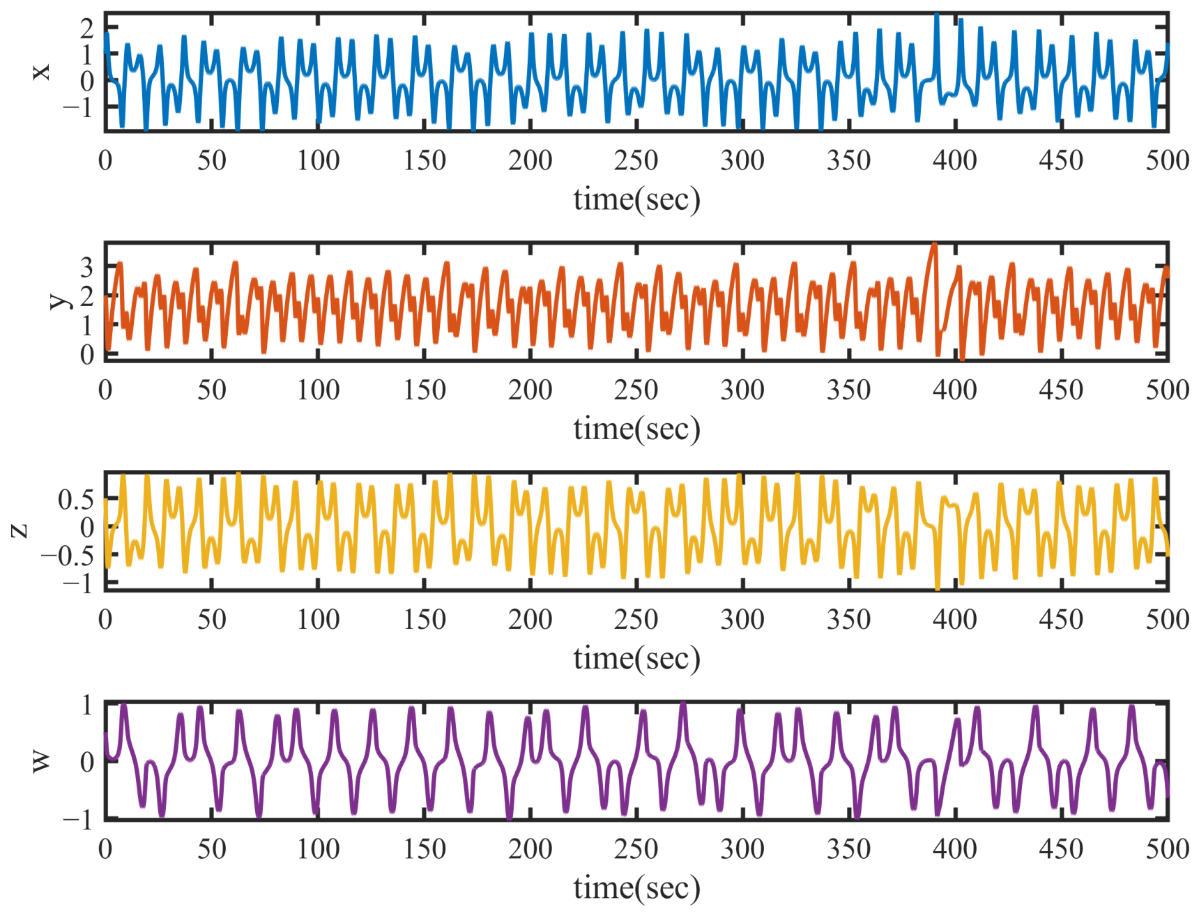
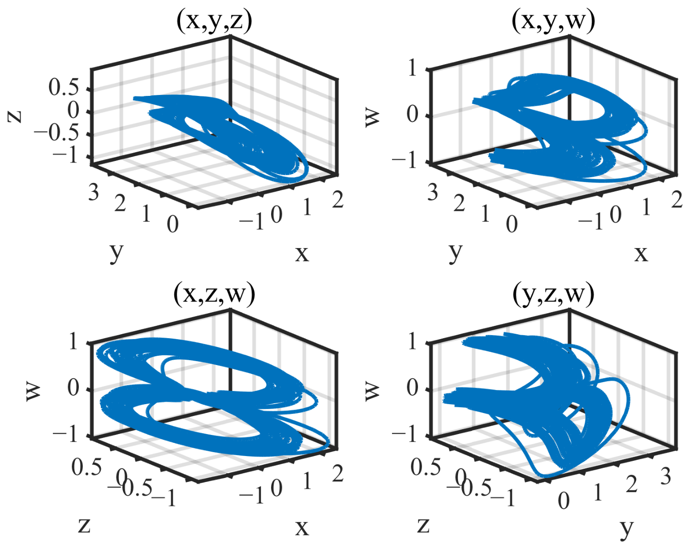
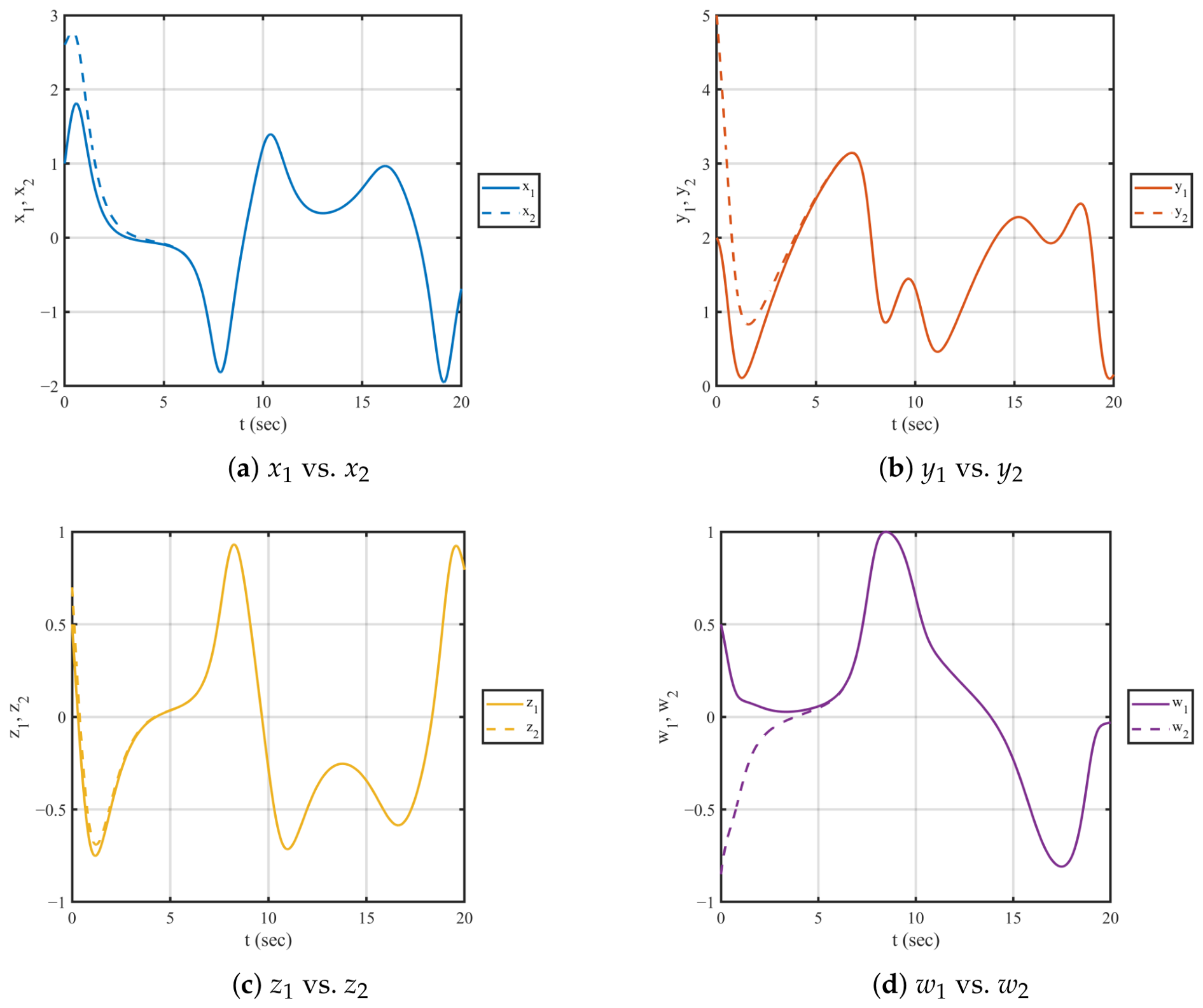
Figure 1 shows representative time series. The oscillations are irregular and do not settle to a fixed point or periodic orbit over the simulated time interval. The 3-D portraits in Figure 2 show different projections of the same four-dimensional trajectory; each projection uses three of the variables $x,y,z,w$ to visualize the geometric structure of the attractor. The projections involving w illustrate how the profit-margin variable changes the geometry of the original three-dimensional finance model and contributes to the double-wing hyperchaotic structure. A nearby-initial-condition test (Figure 3), obtained by perturbing $w\left(0\right)$ by ${10}^{-5}$, shows rapid separation of trajectories, which is consistent with a positive maximal Lyapunov exponent.

Using the QR reorthonormalization method [14,15,16,17,18], we obtain the Lyapunov spectrum

$$\mathit{\lambda }=\{{\lambda }_1,{\lambda }_2,{\lambda }_3,{\lambda }_4\}=\{0.0371809,0.0279798,-0.0363703,-1.13636\}{\mathrm{s}}^{-1},$$

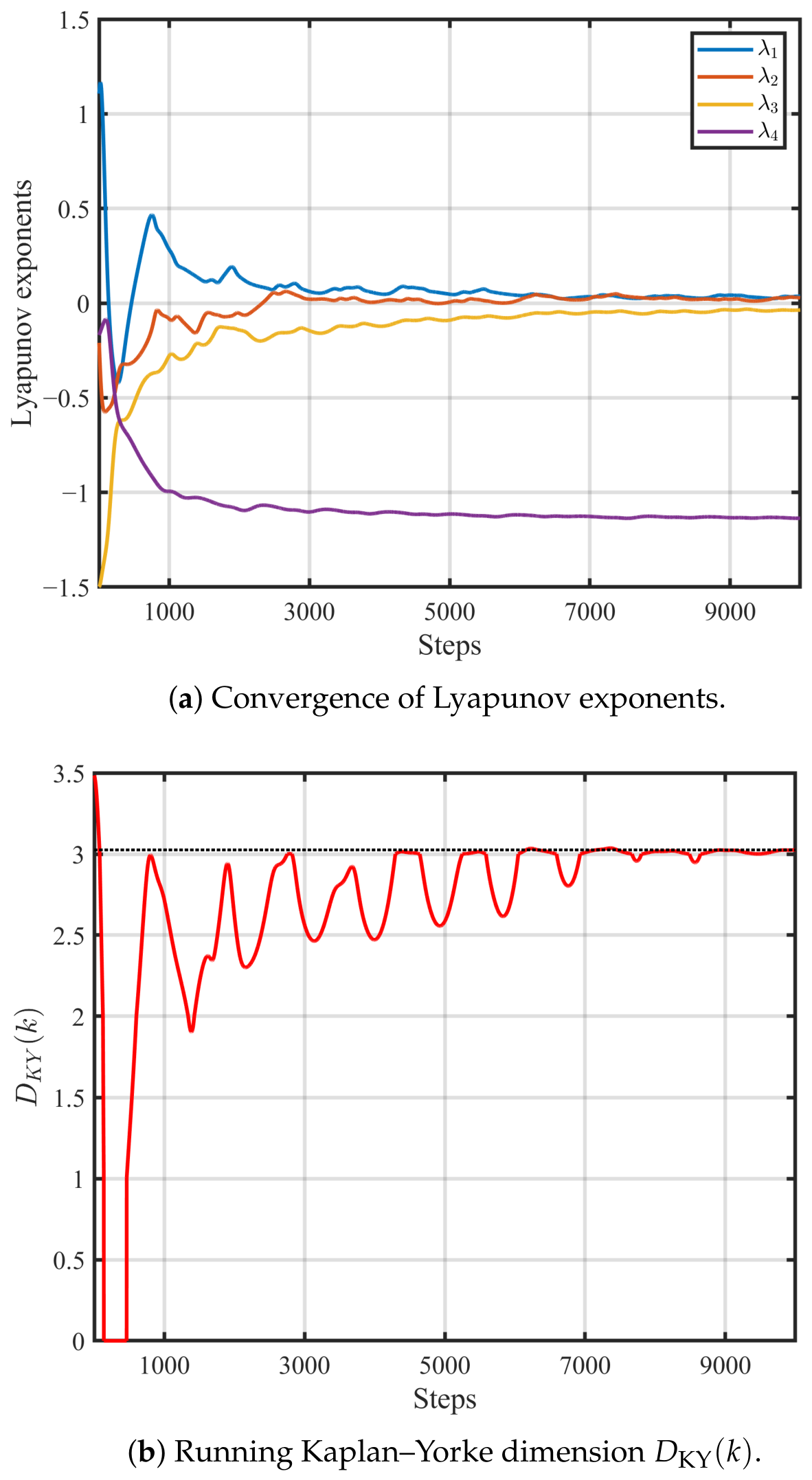
indicating two expanding directions (hyperchaos). The Kaplan–Yorke dimension is

$$D_{\mathrm{KY}}=j+{\displaystyle \frac{{\sum }_{i=1}^j{\lambda }_i}{|{\lambda }_{j+1}|}},j=max\left\{m:{\displaystyle \sum _{i=1}^m}{\lambda }_i\ge 0\right\}=3+{\displaystyle \frac{0.0287904}{1.13636}}\approx 3.025.$$

The value $D_{\mathrm{KY}}\approx 3.025$ means that the attractor has an effective fractal dimension slightly above three. Thus, although the model evolves in four-dimensional phase space, the long-term hyperchaotic attractor occupies a thin fractal set with dimension between three and four. Convergence traces and the running $D_{\mathrm{KY}}\left(k\right)$ are shown in Figure 4. In Figure 4a, two exponents converge to positive values, one approaches a small negative value, and the fourth remains strongly negative, confirming hyperchaotic behavior. The horizontal axis denotes the QR reorthonormalization step number rather than physical time. In Figure 4b, early fluctuations occur because the running exponent estimates are still transient; the curve then approaches the limiting Kaplan–Yorke dimension near 3.025.

Solving

$$z+(y-a)x+w=0,1-by-x^2=0,-x-cz=0,-dxy-kw=0$$

yields three equilibria, provided that $k\ne d$ and ${\alpha }^2>0$:

$$P_0=\left(0,{\displaystyle \frac{1}{b}},0,0\right),P_{\pm }=\left(\pm \alpha ,;y^{\star },;\mp {\displaystyle \frac{\alpha }{c}},;\mp \beta \alpha \right),$$

where

$$y^{\star }={\displaystyle \frac{k(1+ac)}{c(k-d)}},\beta ={\displaystyle \frac{d(1+ac)}{c(k-d)}},{\alpha }^2=1+{\displaystyle \frac{kb(1+ac)}{c(d-k)}}.$$

Here, the superscript ⋆ denotes the equilibrium value of the corresponding state variable. The numerical equilibrium coordinates and the associated Jacobian eigenvalues at the nominal parameter values are summarized in

Table 2. Equilibria and Jacobian eigenvalues (Yu 4-D finance model) at nominal parameters $(a,b,c,d,k)=(0.9,0.2,1.5,0.2,0.17)$. Values are numerical (6 d.p.); all three fixed points are saddles.

Eq.	${\mathit{x}}^{\mathit{\star }}$	${\mathit{y}}^{\mathit{\star }}$	$({\mathit{z}}^{\mathit{\star }},{\mathit{w}}^{\mathit{\star }})$	${spec\left(\mathit{J}\right)|}_{({\mathit{x}}^{\mathit{\star }},{\mathit{y}}^{\mathit{\star }},{\mathit{z}}^{\mathit{\star }},{\mathit{w}}^{\mathit{\star }})}$
$P_0$	$0.000000$	$5.000000$	$(0.000000,0.000000)$	$\{3.643336,0.127808,-0.200000,-1.341144\}$
$P_{-}$	$-1.666000$	$-8.877778$	$(1.110667,-17.400443)$	$\{0.021122,-0.755832,-1.697979,-9.215089\}$
$P_{+}$	$1.666000$	$-8.877778$	$(-1.110667,17.400443)$	$\{0.021122,-0.755832,-1.697979,-9.215089\}$

. These eigenvalues show that $P_0$ and $P_{\pm }$ are saddle points.

Figure 4. Lyapunov spectrum and running $D_{\mathrm{KY}}$ for the Yu 4-D model with $(a,b,c,d,k)=(0.9,0.2,1.5,0.2,0.17)$. The horizontal axis denotes the QR reorthonormalization step number used in the Lyapunov-exponent computation.

Figure 4. Lyapunov spectrum and running $D_{\mathrm{KY}}$ for the Yu 4-D model with $(a,b,c,d,k)=(0.9,0.2,1.5,0.2,0.17)$. The horizontal axis denotes the QR reorthonormalization step number used in the Lyapunov-exponent computation.

3.3. Bifurcation Structure

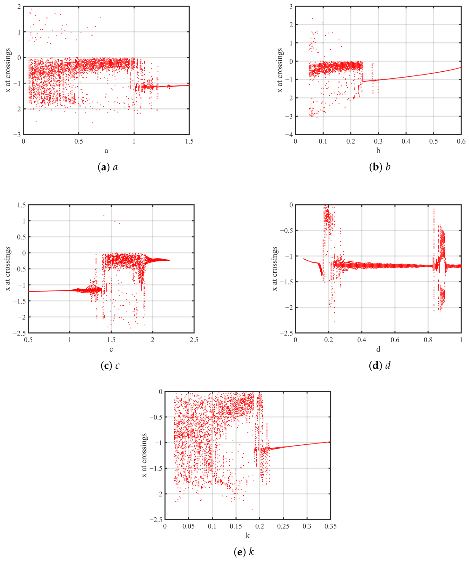
We compute Poincaré sections at $w=0$ with $\dot{w}>0$ while sweeping one parameter at a time and keeping the remaining parameters fixed. For each value of the swept parameter, the full system is integrated, transients are discarded, and up to ${10}^3$ intersections with the Poincaré plane are recorded. Therefore, each vertical slice in Figure 5 corresponds to one complete numerical execution for a fixed parameter value. A finite number of isolated points indicates periodic or low-period motion, whereas a broad scattered cloud indicates chaotic or hyperchaotic motion. 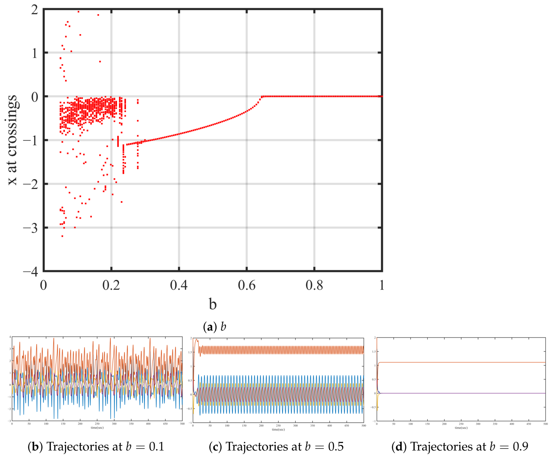Figure 5 summarizes the bifurcation diagrams for $a,b,c,d,$ and k, while Figure 6 gives enlarged views and representative $(w,x)$ trajectories. Within the tested parameter ranges, chaos is observed mainly for $a\le 1$ and $b\le 0.25$; windows of periodicity appear as a or b increase. Chaos is also observed roughly for $1.4\le c\le 1.9$, near $d\approx 0.2$ and $d\approx 0.9$, and for $0<k\le 0.2$.

3.4. Synchronization Experiment Setup

We fix $(a,b,c,d,k)=(0.9,0.2,1.5,0.2,0.17)$ and integrate using ode45 with the same tolerances as above. All controlled simulations use the same initial conditions and solver settings; $C=6$ is used for ABS and $K=3.5$ for SFC. To avoid trivial alignment, master and slave initial conditions are separated:

$$x_1\left(0\right)=1,y_1\left(0\right)=2,z_1\left(0\right)=0.5,w_1\left(0\right)=0.5,$$

(17)

$$x_2\left(0\right)=2.6,y_2\left(0\right)=5,z_2\left(0\right)=0.7,w_2\left(0\right)=-0.85.$$

(18)

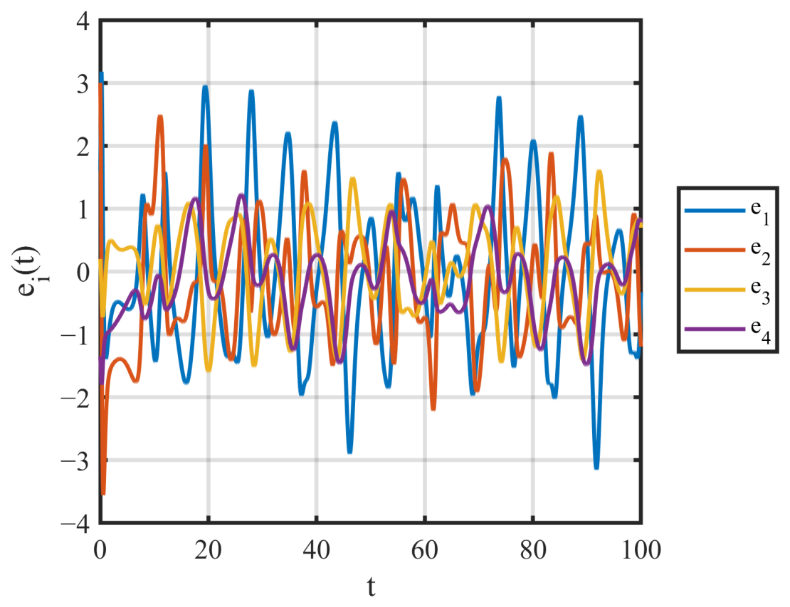
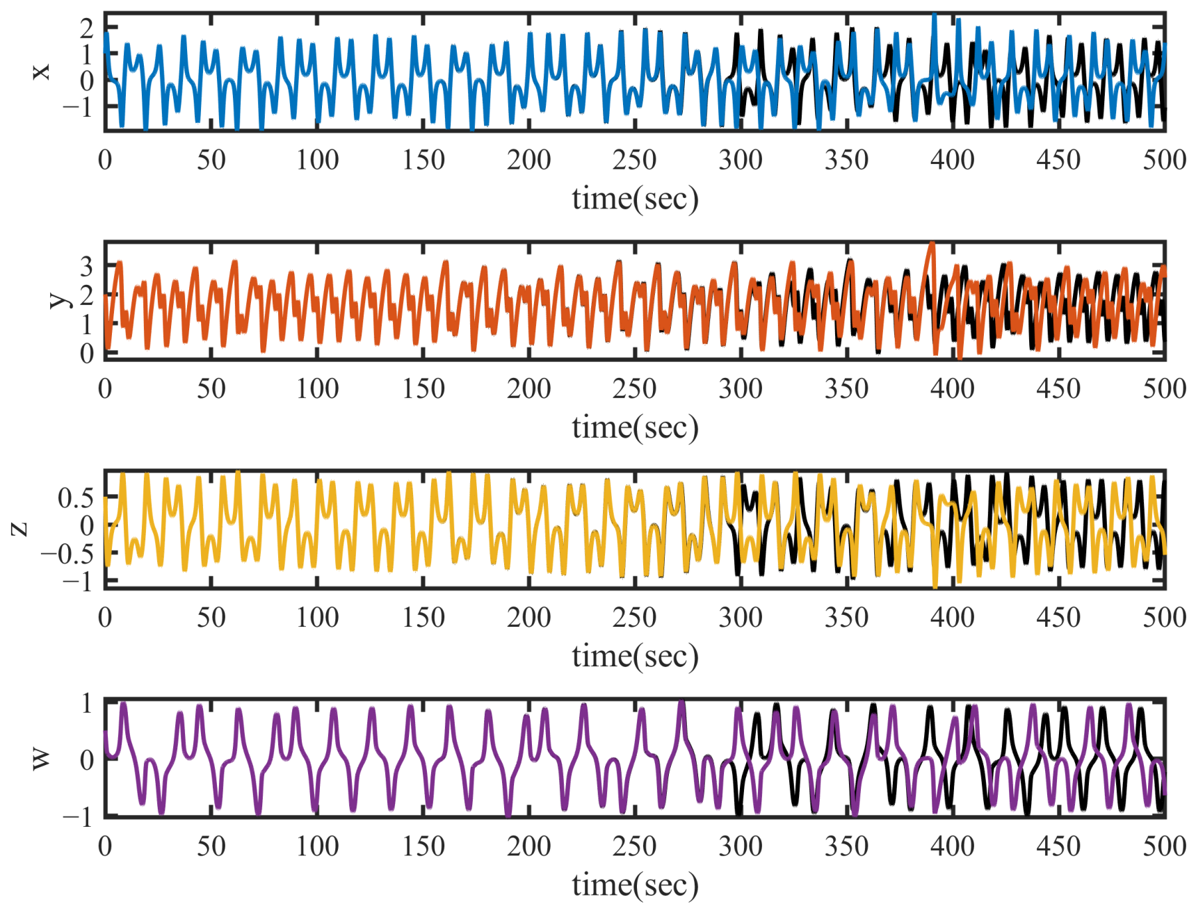
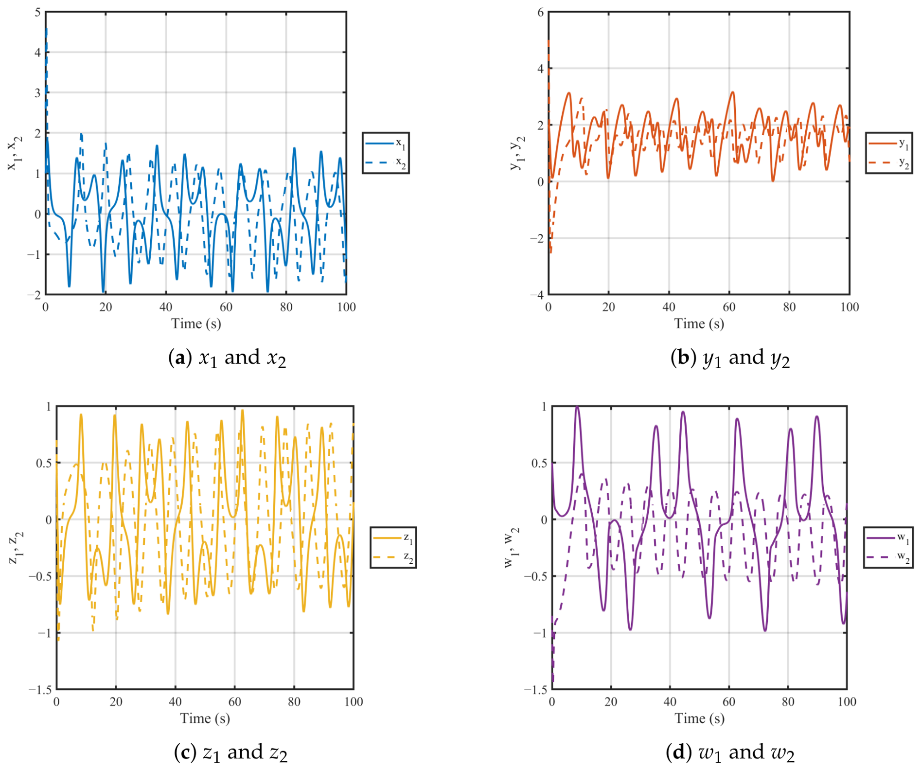
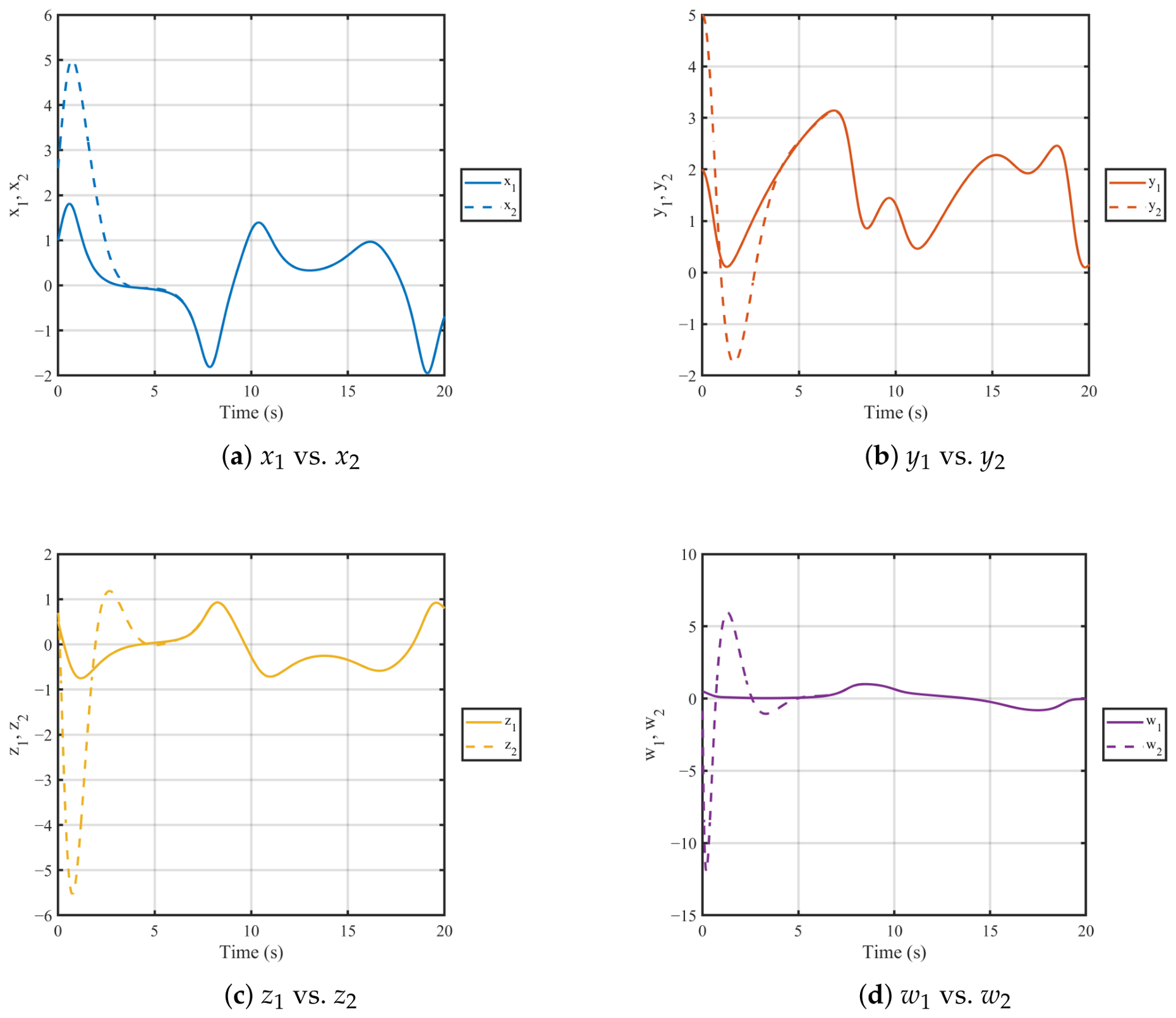
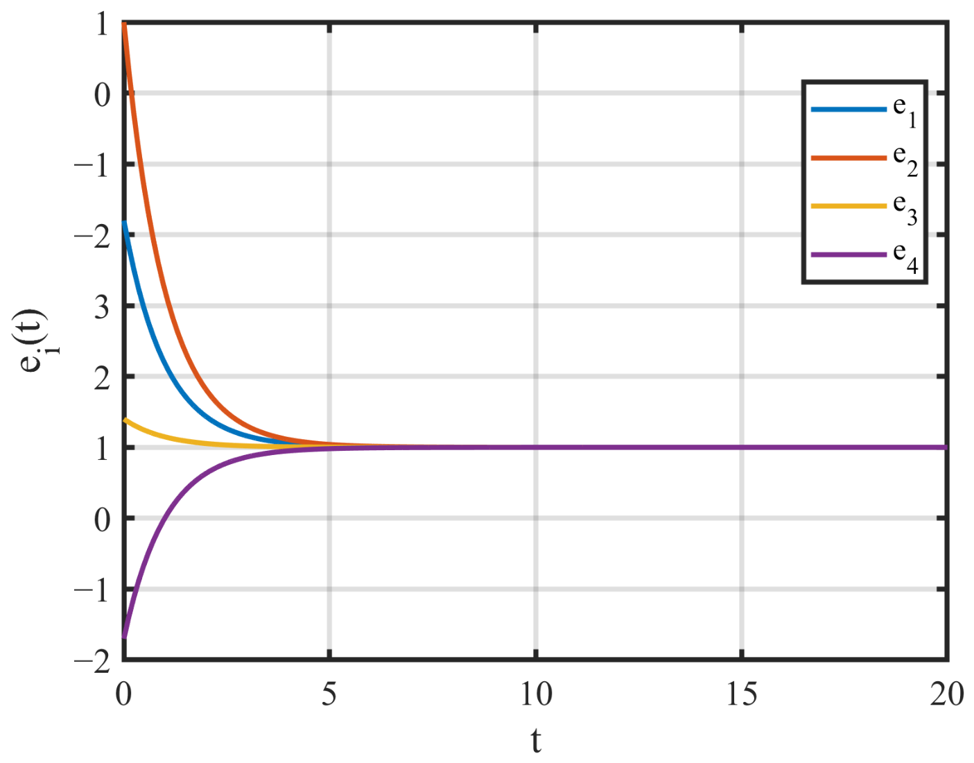
With controllers disabled ($u\equiv 0$) the trajectories diverge (Figure 7); the corresponding uncontrolled error $e=(x_2-x_1,y_2-y_1,z_2-z_1,w_2-w_1)$ is shown in Figure 8.

Figure 6. Bifurcation structure with respect to the parameter b and representative state trajectories. Panel (a) shows the enlarged bifurcation diagram. Panels (b–d) illustrate the corresponding system responses for $b=0.1$, $b=0.5$, and $b=0.9$, respectively. The dense scatter in panel (a) indicates irregular chaotic dynamics, whereas the thin branches correspond to periodic windows. As b increases, the trajectories evolve from (b) chaotic oscillations to (c) periodic motion and finally approach (d) a steady state.

Figure 6. Bifurcation structure with respect to the parameter b and representative state trajectories. Panel (a) shows the enlarged bifurcation diagram. Panels (b–d) illustrate the corresponding system responses for $b=0.1$, $b=0.5$, and $b=0.9$, respectively. The dense scatter in panel (a) indicates irregular chaotic dynamics, whereas the thin branches correspond to periodic windows. As b increases, the trajectories evolve from (b) chaotic oscillations to (c) periodic motion and finally approach (d) a steady state.

3.5. Controller-Gain Selection and Fairness of Comparison

The gains were selected using stability constraints and a small sensitivity study. For the SFC baseline, the Routh–Hurwitz inequalities in Section 2.2.5 require $K>3.46$ at the nominal parameters; therefore $K=3.5$ is the smallest stabilizing value used in the comparison. This choice intentionally favors the baseline by avoiding unnecessarily large feedback. For ABS, any $C>0$ gives the Lyapunov inequality in Proposition 2. The value $C=6$ was selected as a representative moderate gain: it yields fast convergence but avoids increasing the control energy as strongly as larger values. Table 3 shows the stabilization sensitivity for several values of C. The settling time is almost unchanged, while the control effort and peak control magnitude increase with C. This confirms that increasing C is not automatically beneficial from an implementation viewpoint.

Figure 7. Master and slave states before synchronization (parameters as in Section 3.4).

Figure 7. Master and slave states before synchronization (parameters as in Section 3.4).

Figure 8. Uncontrolled error components $e_i\left(t\right)$ before synchronization.

Figure 8. Uncontrolled error components $e_i\left(t\right)$ before synchronization.

Table 3. Sensitivity of ABS stabilization to the gain C on $t\in [0,100]$ s.

C	ts(2%) [s]	Overshoot [%]	${\int }_0^{100}{\parallel \mathit{u}\left(\mathit{t}\right)\parallel }_2^2\mathit{dt}$	${max}_{\mathit{t}}{\parallel \mathit{u}\left(\mathit{t}\right)\parallel }_2$
2	5.92	226.2	$6.37\times {10}^2$	61.1
4	5.93	270.5	$8.79\times {10}^2$	91.0
6	5.93	301.0	$1.11\times {10}^3$	121.0
8	5.92	323.7	$1.35\times {10}^3$	151.0
10	5.92	341.4	$1.57\times {10}^3$	181.0

Table 3. Sensitivity of ABS stabilization to the gain C on $t\in [0,100]$ s.

C	ts(2%) [s]	Overshoot [%]	${\int }_0^{100}{\parallel \mathit{u}\left(\mathit{t}\right)\parallel }_2^2\mathit{dt}$	${max}_{\mathit{t}}{\parallel \mathit{u}\left(\mathit{t}\right)\parallel }_2$
2	5.92	226.2	$6.37\times {10}^2$	61.1
4	5.93	270.5	$8.79\times {10}^2$	91.0
6	5.93	301.0	$1.11\times {10}^3$	121.0
8	5.92	323.7	$1.35\times {10}^3$	151.0
10	5.92	341.4	$1.57\times {10}^3$	181.0

3.6. Controller Performance: Stabilization

We compare active backstepping (ABS) with speed-feedback (SFC).

3.6.1. ABS (Global Stabilization)

Proposition 2

(Global exponential stabilization under ABS). Consider the controlled Yu 4-D finance model (5) with the active-backstepping law (9) for any gain $C>0$. Then the origin is globally exponentially stable. In particular, there exist constants $\alpha =1$ and $\kappa \ge 1$ (depending only on the fixed nonsingular transformation T used in Section 2.2.2) such that, for all $t\ge 0$,

$${∥\left(x\right(t),y(t),z(t),w(t\left)\right)∥}_2\le \kappa e^{-\alpha t}{∥\left(x\right(0),y(0),z(0),w(0\left)\right)∥}_2.$$

Proof. 

With the static prefeedback (6) the plant becomes the integrator chain (7). Define ${\phi }_1=x$, ${\phi }_2=x+y$, ${\phi }_3=2x+2y+z$, ${\phi }_4=3x+5y+3z+w$ and the quadratic Lyapunov function $V=\frac{1}{2}{\sum }_{i=1}^4{\phi }_i^2$. Along (7), choosing v as in (8) yields

$$\dot{V}=-{\phi }_1^2-{\phi }_2^2-{\phi }_3^2-(1+C){\phi }_4^2\le -2V,$$

so $V\left(t\right)\le V\left(0\right)e^{-2t}$ and ${\parallel \phi \left(t\right)\parallel }_2\le e^{-t}{\parallel \phi \left(0\right)\parallel }_2$ for all $t\ge 0$. Since $\phi =T{\left[xyzw\right]}^{\top }$ with a fixed lower-triangular nonsingular T, norm equivalence gives ${\parallel \left[xyzw\right]}^{\top }{\parallel }_2\le \parallel T^{-1}{\parallel }_2{\parallel \phi \parallel }_2\le \parallel T^{-1}{\parallel }_2{e}^{-t}{\parallel \phi \left(0\right)\parallel }_2\le \parallel T^{-1}{\parallel }_2{\parallel T\parallel }_2{e}^{-t}{\parallel {\left[x\left(0\right)y\left(0\right)z\left(0\right)w\left(0\right)\right]}^{\top }\parallel }_2$. Letting $\kappa :=\parallel T^{-1}{\parallel }_2{\parallel T\parallel }_2$ and $\alpha :=1$ proves the claim. □

The term “global” in Proposition 2 refers to the ideal mathematical closed loop with exact full-state feedback, exact model cancellation, and no actuator saturation, measurement delay, or parameter mismatch. When these nonidealities are introduced, the simulations in Section 3.8 should be interpreted as numerical robustness evidence rather than as an ISS or $H_{\infty }$ robustness proof.

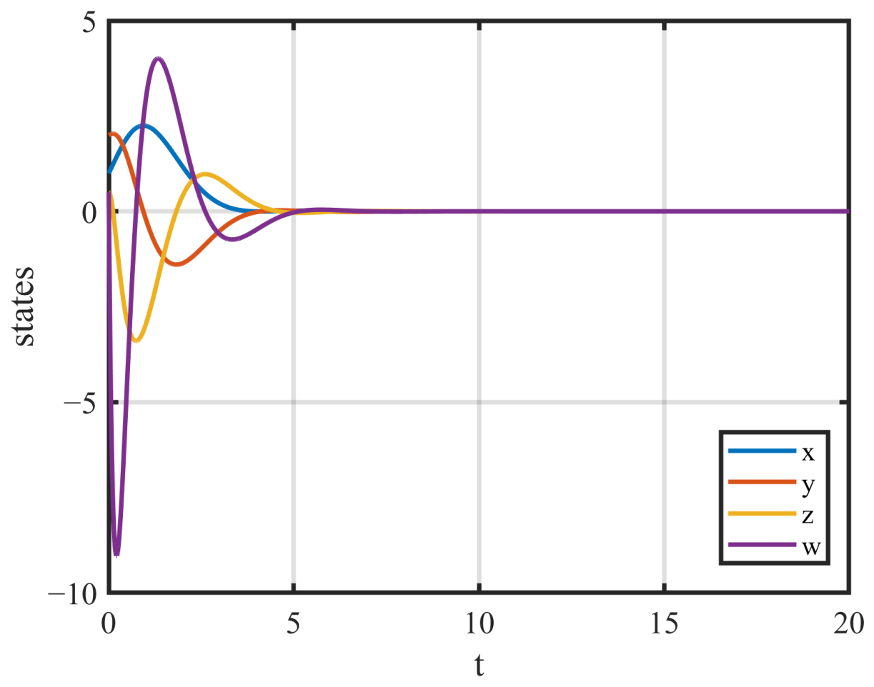
With the ABS stabilizer in (9) and $C=6$, the state vector $\mathbf{x}\left(t\right)={(x\left(t\right),y\left(t\right),z\left(t\right),w\left(t\right))}^{\top }$ converges exponentially to the origin, as shown in Figure 9. An envelope fit of ${log\parallel \mathbf{x}\left(t\right)\parallel }_2$ over $t\in [0.5,100]$ s yields ${\rho }_{\mathrm{emp}}\approx 0.330{\mathrm{s}}^{-1}$, consistent with the Lyapunov-based convergence estimate.

Using the shifted model in Section 2.2.5 and the speed-feedback controller with $K=3.5$, the Routh–Hurwitz conditions are satisfied. The corresponding linearized eigenvalues at $P_0$ are

$$-0.2000,-1.0233,-0.0233\pm 0.7808i.$$

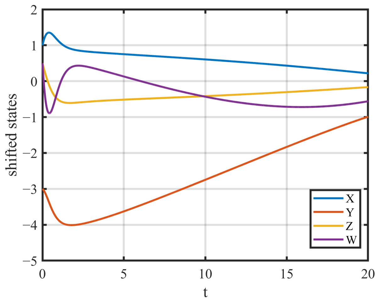
Thus, $P_0$ is locally asymptotically stable under the speed-feedback controller. The numerical response in Figure 10 confirms convergence, although the decay is slower and mildly oscillatory compared with the ABS-controlled system.

3.6.2. Stabilization Metrics

Using a common window $t\in [0.5,100]$ s and envelope-based fits on ${\parallel x\left(t\right)\parallel }_2$, ABS achieves a much shorter settling time than SFC. However, this faster convergence is accompanied by higher transient overshoot and larger integrated control energy. By contrast, SFC is more economical but remains outside the 2% band over the simulated time interval. The corresponding stabilization benchmarks are summarized in

Table 4. Stabilization benchmarks on $t\in [0.5,100]$ s (envelope fits).

Metric	ABS ($\mathit{C}=6$)	SFC ($\mathit{K}=3.5$)
Settling time $t_s(2\%)$ [s]	5.93	>100
Overshoot $\%OS$ [%]	301.0	40.8
Rate $\rho$ [${\mathrm{s}}^{-1}$]	0.330	0.0025
${\displaystyle {\int }_0^{100}{\parallel u\left(t\right)\parallel }_2^{2}dt}$	∼1.11 $\times {10}^3$	∼7.8 $\times {10}^1$
CPU time [s]	0.127	0.050

.

3.7. Controller Performance: Synchronization

We compare ABS synchronization (Section 2.2.3) with active control (AC, Section 2.2.4). Under the same initial conditions, parameter values, and solver settings, both methods achieve drive–response synchronization.

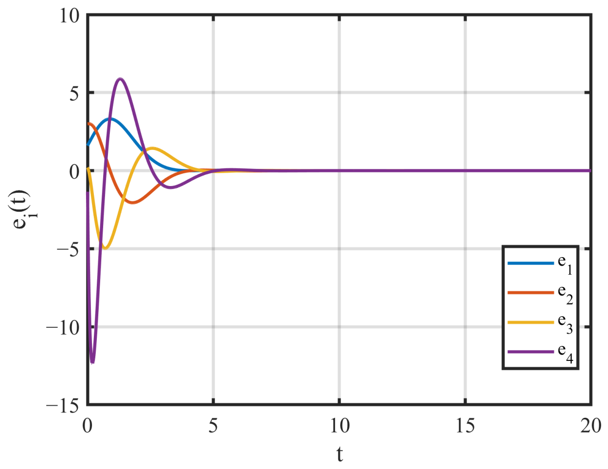
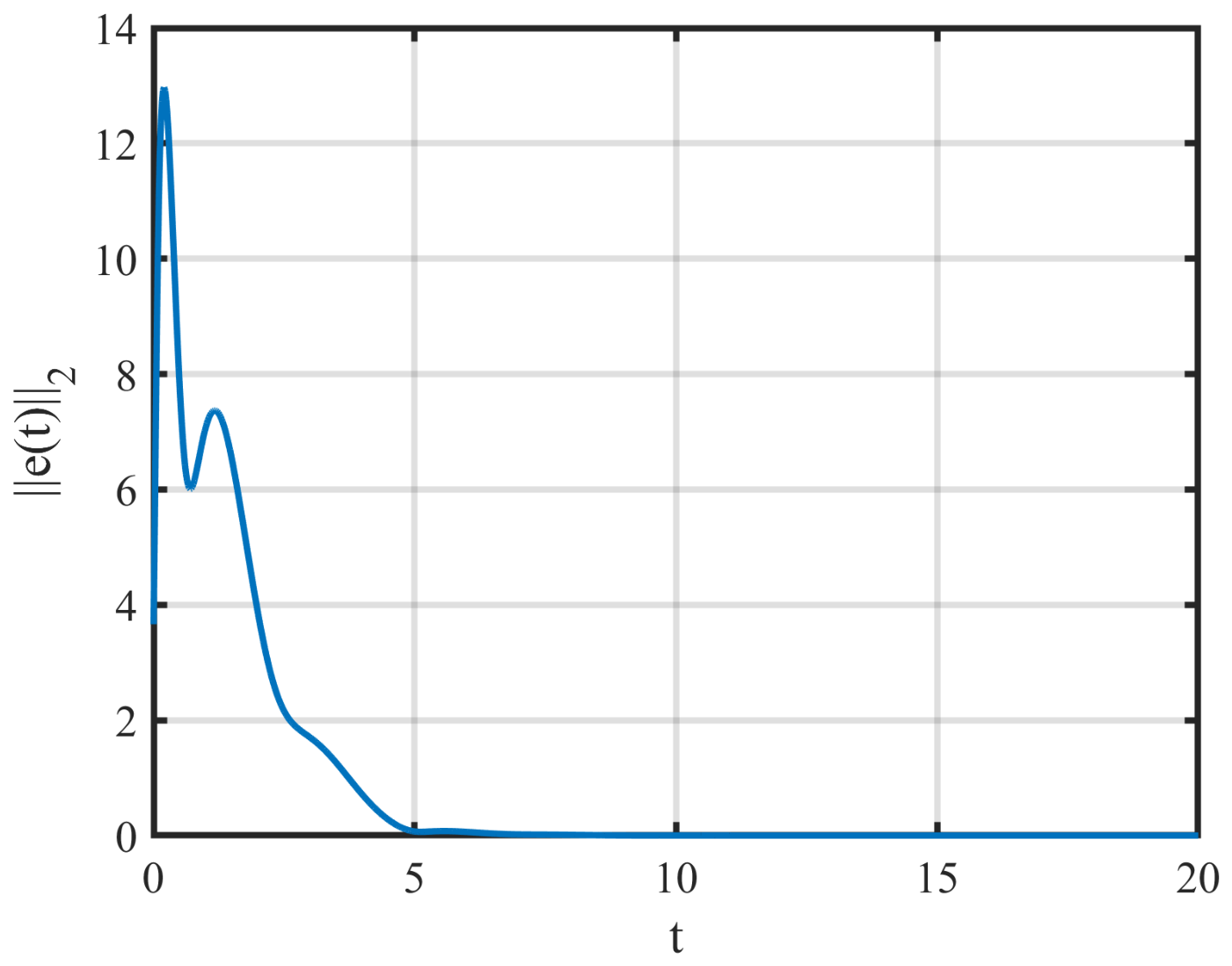
For ABS synchronization, the prefeedback law (10) together with the terminal control law (11) is used with $C=6$. The state trajectories align and the synchronization error decays exponentially, as shown in Figure 11, Figure 12 and Figure 13.

For AC synchronization, the cancellation-plus-gain law (16) is used with $A=-I_4$. In this case, the closed-loop error system satisfies

$$\dot{e}=-e,$$

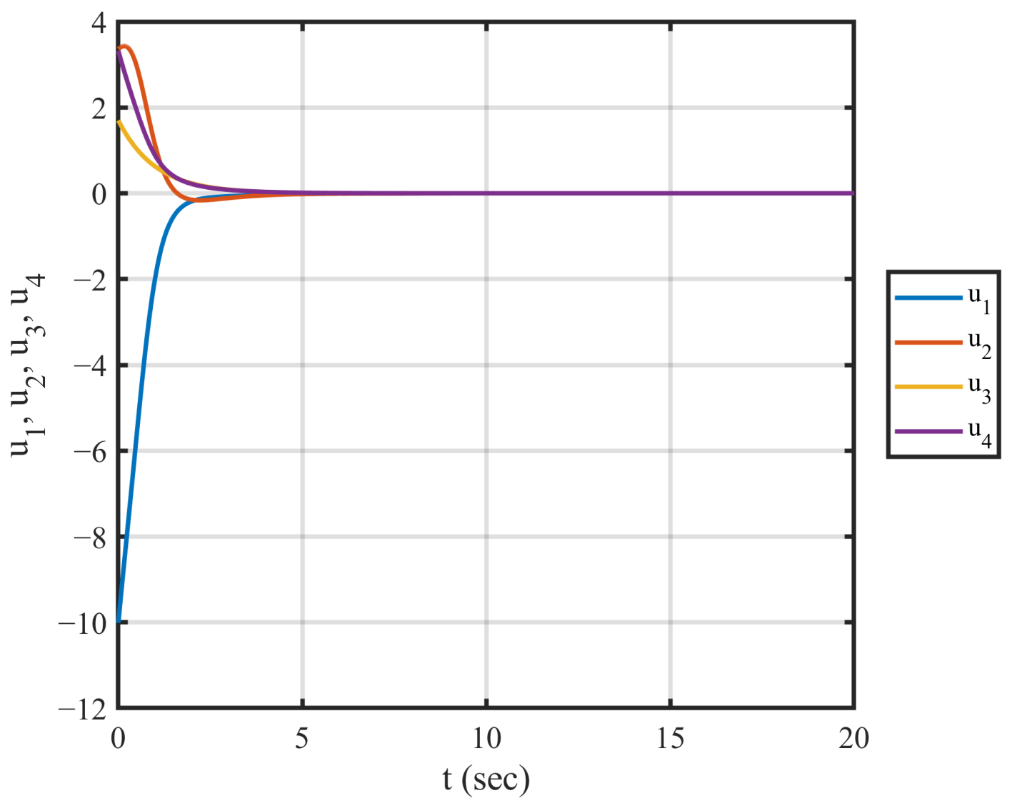
and hence ${\parallel e\left(t\right)\parallel }_2\le e^{-t}{\parallel e\left(0\right)\parallel }_2$. The corresponding error components and synchronized state trajectories are shown in Figure 14, Figure 15 and Figure 16.

Using the common window $t\in [0.5,100]$ s and envelope-based fits on ${\parallel e\left(t\right)\parallel }_2$, AC gives the shorter settling time and zero overshoot in the nominal case. ABS also achieves exponential synchronization, with a comparable fitted decay rate, but it produces a larger transient response. Thus, in the nominal synchronization experiment, AC provides the smoother and more efficient synchronization performance, while ABS offers a Lyapunov-based nonlinear alternative. The corresponding nominal synchronization benchmarks are summarized in Table 5.

Figure 11. ABS synchronization: aligned states under (10) and (11).

Figure 11. ABS synchronization: aligned states under (10) and (11).

Figure 12. ABS synchronization: error components $e_i\left(t\right)$.

Figure 12. ABS synchronization: error components $e_i\left(t\right)$.

Table 5. Nominal synchronization benchmarks on $t\in [0.5,100]$ s (envelope fits).

Metric	ABS ($\mathit{C}=6$)	AC ($\mathit{A}=-{\mathit{I}}_4$)
Settling time $t_s(2\%)$ [s]	5.79	3.91
Overshoot $\%OS$ [%]	254.1	0.0
Rate $\rho$ [${\mathrm{s}}^{-1}$]	1.04	1.00

Table 5. Nominal synchronization benchmarks on $t\in [0.5,100]$ s (envelope fits).

Metric	ABS ($\mathit{C}=6$)	AC ($\mathit{A}=-{\mathit{I}}_4$)
Settling time $t_s(2\%)$ [s]	5.79	3.91
Overshoot $\%OS$ [%]	254.1	0.0
Rate $\rho$ [${\mathrm{s}}^{-1}$]	1.04	1.00

Figure 13. ABS synchronization: average error $e_{\mathrm{avg}}\left(t\right)={\parallel e\left(t\right)\parallel }_2$.

Figure 13. ABS synchronization: average error $e_{\mathrm{avg}}\left(t\right)={\parallel e\left(t\right)\parallel }_2$.

Figure 14. AC synchronization: error components $e_i\left(t\right)$.

Figure 14. AC synchronization: error components $e_i\left(t\right)$.

Actuator Magnitude

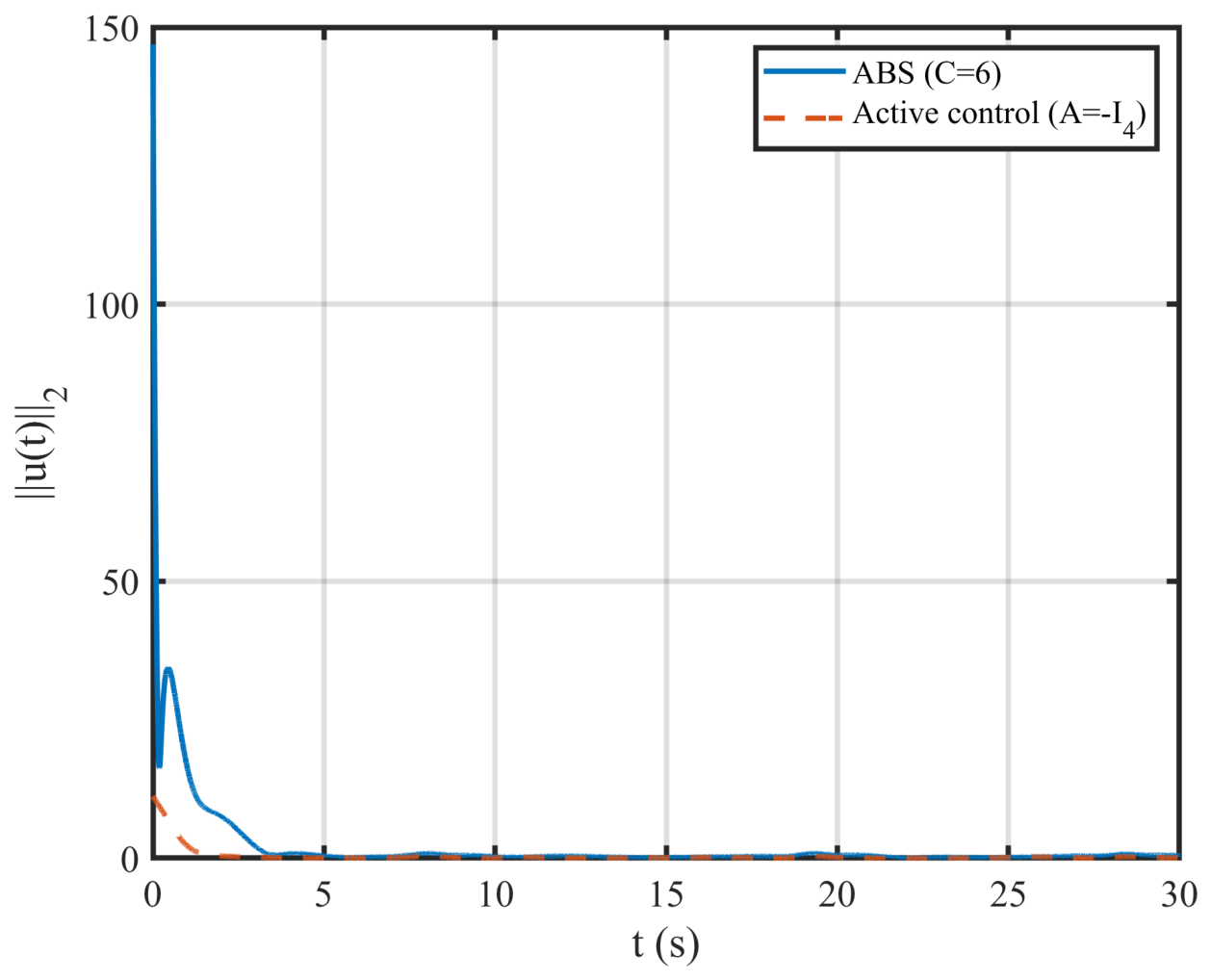
To assess implementation feasibility,

Table 6. Peak and RMS control-input magnitudes in nominal synchronization on $t\in [0,100]$ s.

	Peak $|{\mathit{u}}_{\mathit{i}}|$				RMS ${\mathit{u}}_{\mathit{i}}$
Method	${\mathit{u}}_{\mathbf{1}}$	${\mathit{u}}_{\mathbf{2}}$	${\mathit{u}}_{\mathbf{3}}$	${\mathit{u}}_{\mathbf{4}}$	${\mathit{u}}_{\mathbf{1}}$	${\mathit{u}}_{\mathbf{2}}$	${\mathit{u}}_{\mathbf{3}}$	${\mathit{u}}_{\mathbf{4}}$
ABS ($C=6$)	5.41	17.20	12.96	146.73	0.407	1.745	1.046	3.790
AC ($A=-I_4$)	10.01	3.43	1.70	3.32	0.626	0.283	0.120	0.216

reports the peak and RMS control magnitudes for the nominal synchronization experiment. The AC law requires much smaller control amplitudes than ABS. In particular, the fourth ABS input has the largest transient demand because it contains the terminal backstepping correction. This explains why ABS can be attractive for fast nonlinear convergence but less attractive when actuator limits or energy budgets are restrictive.

3.8. Robustness to Parameter Mismatch and Measurement Noise

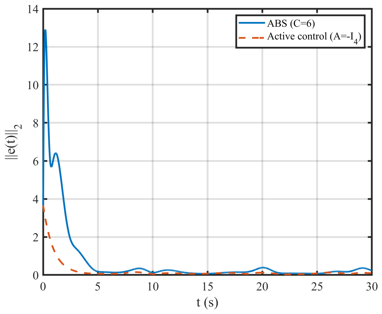
We test realizability under (i) $\pm 10\%$ parameter mismatch on $(a,b,c,d,k)$ in the response system and (ii) additive measurement noise $\eta \left(t\right)\sim \mathcal{N}(0,{\sigma }^2)$ with $\sigma ={10}^{-3}$ on each measured state; the master uses nominal parameters. The noisy measurements are used in the control law, while the reported error is computed from the true simulated states. In the numerical tests with simultaneous parameter mismatch and measurement noise, both controllers produce bounded trajectories and decaying synchronization error (Figure 17). ABS gives the larger envelope-based decay rate, whereas AC requires substantially lower control energy (Figure 18). These tests are not intended to replace a formal ISS robustness proof; rather, they indicate how the ideal cancellation-based laws behave under moderate implementation errors. The corresponding robust synchronization metrics, including envelope-fit rate, e-folding time, control energy, and CPU time, are summarized in Table 7.

Figure 15. AC synchronization: aligned state trajectories.

Figure 15. AC synchronization: aligned state trajectories.

Figure 16. AC synchronization: control inputs $(u_1,u_2,u_3,u_4)$.

Figure 16. AC synchronization: control inputs $(u_1,u_2,u_3,u_4)$.

Table 7. Robust synchronization under $\pm 10\%$ mismatch and $\sigma ={10}^{-3}$ noise (envelope-fit rates on $t\in [0,100]$ s).

Metric	ABS ($\mathit{C}=6$)	AC ($\mathit{A}=-{\mathit{I}}_4$)
${\rho }_{\mathrm{env}}$ [${\mathrm{s}}^{-1}$]	0.0103	0.0044
E-folding time $1/{\rho }_{\mathrm{env}}$ [s]	97.6	226.5
${\displaystyle {\int }_0^{100}{\parallel u\left(t\right)\parallel }_2^{2}dt}$	$2.10\times {10}^3$	$6.05\times {10}^1$
CPU time [s]	396.1	124.5

Table 7. Robust synchronization under $\pm 10\%$ mismatch and $\sigma ={10}^{-3}$ noise (envelope-fit rates on $t\in [0,100]$ s).

Metric	ABS ($\mathit{C}=6$)	AC ($\mathit{A}=-{\mathit{I}}_4$)
${\rho }_{\mathrm{env}}$ [${\mathrm{s}}^{-1}$]	0.0103	0.0044
E-folding time $1/{\rho }_{\mathrm{env}}$ [s]	97.6	226.5
${\displaystyle {\int }_0^{100}{\parallel u\left(t\right)\parallel }_2^{2}dt}$	$2.10\times {10}^3$	$6.05\times {10}^1$
CPU time [s]	396.1	124.5

Figure 17. Robust synchronization: error norm ${\parallel e\left(t\right)\parallel }_2$ for ABS ($C=6$) and AC ($A=-I_4$) with $\pm 10\%$ mismatch and $\sigma ={10}^{-3}$ noise.

Figure 17. Robust synchronization: error norm ${\parallel e\left(t\right)\parallel }_2$ for ABS ($C=6$) and AC ($A=-I_4$) with $\pm 10\%$ mismatch and $\sigma ={10}^{-3}$ noise.

The robustness simulations suggest a clear trade-off. ABS gives faster envelope decay under the tested perturbations, but it requires considerably higher actuation energy. AC is more economical and produces smoother transients, making it preferable when actuator limits or energy budgets are important. ABS is preferable when faster decay is the main objective. The reported CPU times correspond to the noisy robustness simulations and depend on the solver tolerances and hardware used. Larger mismatch levels, colored noise, sensor delays, and hard saturation constraints remain important extensions; the present results should therefore be viewed as moderate-perturbation numerical evidence rather than a complete robustness characterization.

Figure 18. Robust synchronization: control effort ${\parallel u\left(t\right)\parallel }_2$. ABS uses a larger transient burst; AC is substantially more economical.

Figure 18. Robust synchronization: control effort ${\parallel u\left(t\right)\parallel }_2$. ABS uses a larger transient burst; AC is substantially more economical.

3.9. Contextual Comparison with Established Controller Families

In addition to the numerical comparison with SFC,

Table 8. Qualitative comparison with established controller families for the Yu four-dimensional finance model.

Controller Family	Main Strength	Main Limitation/Trade-Off
Speed-feedback control [3]	Simple local stabilizer around $P_0$	Linearized/local design; slow convergence in the present benchmark
Recursive backstepping [6]	Lyapunov-based nonlinear design	Requires recursive construction and may have larger transients
Backstepping/sliding-mode variants [6,7]	Improved robustness and fast response	May require boundary-layer/chattering-reduction tuning
Single-controller schemes [10]	Low-dimensional actuation structure	Typically less flexible and may be sensitive to operating point
Adaptive/robust synchronization [8,9]	Handles parameter uncertainty more explicitly	More complex adaptation law and additional tuning parameters
nAC/ABS in this work	Unified stabilization–synchronization benchmark with rate, energy, CPU, and actuator metrics	Exact-cancellation designs require measured states and may demand large inputs without saturation handling

summarizes how the proposed AC and ABS designs relate to established controller families previously reported for the Yu finance model. This table is qualitative because several published controllers use different targets, assumptions, gains, and performance metrics. Therefore, a direct numerical ranking without reimplementation would be misleading. The main purpose is to clarify where the proposed methods fit in the broader control landscape.

4. Comparative Performance Evaluation

The comparative evaluation highlights the trade-offs among the proposed controllers and the speed-feedback baseline. For stabilization, ABS achieves a substantially shorter settling time and a larger fitted decay rate than SFC, confirming the effectiveness of the nonlinear backstepping design. However, this improvement is obtained at the cost of higher transient overshoot and larger integrated control energy. SFC is structurally simpler and more economical, but its convergence is considerably slower under the nominal parameter setting.

For synchronization, both AC and ABS achieve exponential decay of the synchronization error. AC gives smoother transients, lower control effort, and faster nominal settling, whereas ABS provides a Lyapunov-based nonlinear design with strong convergence properties. Under parameter mismatch and additive measurement noise, both controllers remain bounded and show decaying synchronization error in the tested simulations. Overall, AC is preferable when low control energy and smooth synchronization are prioritized, while ABS is preferable when a nonlinear Lyapunov-based stabilization framework is required.

5. Conclusions

This paper investigated the stabilization and drive–response synchronization of the Yu four-dimensional hyperchaotic finance system using active control and active backstepping strategies. The uncontrolled model was first examined through phase portraits, Lyapunov exponents, equilibrium analysis, and bifurcation diagrams, confirming the presence of periodic, chaotic, and hyperchaotic regimes under different parameter values.

For stabilization, an active-backstepping controller was constructed by transforming the system into an integrator-chain form. A Lyapunov argument established global exponential convergence of the controlled states to the origin. Numerical simulations showed that, compared with the classical speed-feedback baseline, the proposed ABS controller gives faster convergence, although at the cost of higher control effort.

For synchronization, both active control and active backstepping were implemented in a drive–response configuration. The AC design gives a simple cancellation-plus-gain structure with exponential error decay, while the ABS design provides a nonlinear Lyapunov-based alternative. The numerical results indicate that AC gives smoother and more energy-efficient synchronization, whereas ABS offers a rigorous nonlinear synchronization framework.

Overall, the results demonstrate that active control and active backstepping are effective tools for suppressing hyperchaotic behavior in the four-dimensional finance model. The study also highlights a practical trade-off between convergence speed, control energy, and implementation complexity.

Future Work

Future work should consider input constraints, actuator saturation, colored noise, sensor delay, stochastic disturbances, and noise filtering. A formal ISS or $H_{\infty }$ robustness analysis would be valuable for quantifying robustness beyond the moderate perturbation tests reported here. Further extensions may include fractional-order or time-delay versions of the model, adaptive or surrogate-assisted gain selection, and validation using real financial time-series data to assess the practical relevance of the proposed control strategies.

References

- Grandmont, J.M. On endogenous competitive business cycles. Econom. J. Econom. Soc. 1985, 53, 995–1045. [Google Scholar] [CrossRef] [Scilit]
- Ma, J.-H.; Chen, Y.-S. Study for the bifurcation topological structure and the global complicated character of a kind of nonlinear finance system (I). Appl. Math. Mech. 2001, 22, 1240–1251. [Google Scholar] [CrossRef] [Scilit]
- Yu, H.; Cai, G.; Li, Y. Dynamic analysis and control of a new hyperchaotic finance system. Nonlinear Dyn. 2012, 67, 2171–2182. [Google Scholar]
- Liu, Y.; Li, T.; Zhou, Z.; Ren, W.; Lin, W. Real-World Nighttime Image Dehazing via Bayesian-Based Fractional-Order Variational Model. IEEE Trans. Image Process. 2026, 35, 4673–4685. [Google Scholar] [CrossRef] [Scilit] [PubMed]
- Mahalakshmi, K.; Nagarajan, S. Comprehensive Review and Analysis of Image Encryption Techniques. IEEE Access 2025, 13, 109783–109813. [Google Scholar] [CrossRef] [Scilit]
- Hu, P.; Cai, G.L.; Yao, L.; Fang, X.L. Recursive backstepping nonlinear control and sliding mode control of a novel hyperchaotic finance system. Adv. Mater. Res. 2013, 756, 775–780. [Google Scholar] [CrossRef] [Scilit]
- Cai, G.; Ding, Y.; Chen, Q. SMC Chaos Control of a Novel Hyperchaotic Finance System Using a New Chatter Free Sliding Mode Control. Proc. J. Phys. Conf. Ser. 2019, 1187, 032103. [Google Scholar] [CrossRef] [Scilit]
- Karimi, M.; Saberi Nik, H. A piecewise spectral method for solving the chaotic control problems of hyperchaotic finance system. Int. J. Numer. Model. Electron. Netw. Devices Fields 2018, 31, e2284. [Google Scholar] [CrossRef] [Scilit]
- Shafiq, M.; Ahmad, I. Robust synchronization of four-dimensional chaotic finance systems with unknown parametric uncertainties. Automatika 2024, 65, 217–234. [Google Scholar]
- He, P.; Li, Y. Control and synchronization of a hyperchaotic finance system via single controller scheme. Int. J. Intell. Comput. Cybern. 2015, 8, 330–344. [Google Scholar] [CrossRef] [Scilit]
- Ott, E.; Grebogi, C.; Yorke, J.A. Controlling chaos. Phys. Rev. Lett. 1990, 64, 1196. [Google Scholar] [CrossRef] [Scilit] [PubMed]
- Pecora, L.M.; Carroll, T.L. Synchronization in chaotic systems. Phys. Rev. Lett. 1990, 64, 821. [Google Scholar] [CrossRef] [Scilit] [PubMed]
- Akter, M.T.; Tarammim, A.; Hussen, S. Chaos control and synchronization of modified Lorenz system using active control and backstepping scheme. In Waves in Random and Complex Media; Taylor & Francis: Oxfordshire, UK, 2023; pp. 1–20. [Google Scholar]
- Benettin, G.; Galgani, L.; Giorgilli, A.; Strelcyn, J.M. Lyapunov characteristic exponents for smooth dynamical systems and for Hamiltonian systems; A method for computing all of them. Part 1: Theory. Meccanica 1980, 15, 9–20. [Google Scholar] [CrossRef] [Scilit]
- Benettin, G.; Galgani, L.; Giorgilli, A.; Strelcyn, J.M. Lyapunov characteristic exponents for smooth dynamical systems and for Hamiltonian systems; A method for computing all of them. Part 2: Numerical application. Meccanica 1980, 15, 21–30. [Google Scholar] [CrossRef] [Scilit]
- Shimada, I.; Nagashima, T. A numerical approach to ergodic problem of dissipative dynamical systems. Prog. Theor. Phys. 1979, 61, 1605–1616. [Google Scholar] [CrossRef] [Scilit]
- Sandri, M. Numerical calculation of Lyapunov exponents. Math. J. 1996, 6, 78–84. [Google Scholar]
- Wolf, A.; Swift, J.B.; Swinney, H.L.; Vastano, J.A. Determining Lyapunov exponents from a time series. Phys. D Nonlinear Phenom. 1985, 16, 285–317. [Google Scholar] [CrossRef] [Scilit]
- Guo, Y.; Nath, P.; Mahadevan, S.; Witherell, P. Active learning for adaptive surrogate model improvement in high-dimensional problems. Struct. Multidiscip. Optim. 2024, 67, 122. [Google Scholar] [CrossRef] [Scilit] [PubMed]
- Cavoretto, R.; Haider, A.; Lancellotti, S.; Mezzanotte, D.; Noorizadegan, A. Adaptive residual subsampling algorithms for kernel interpolation based on cross validation techniques. Constr. Math. Anal. 2024, 7, 76–92. [Google Scholar] [CrossRef] [Scilit]
Figure 1.
Time series of (
1) for
and
. The oscillations remain irregular and do not converge to a fixed point or periodic orbit over the simulated time interval.
Figure 2.
3-D phase portraits (transient s removed). Each panel shows a different three-variable projection of the same four-dimensional trajectory, illustrating how the variables jointly form the hyperchaotic attractor.
Figure 3.
Sensitivity to initial conditions. Original IC: ; perturbed IC (black): . Trajectories from nearby initial conditions, differing only by a perturbation in , separate rapidly, consistent with a positive maximal Lyapunov exponent.
Figure 5.
Bifurcation diagrams via the Poincaré section (, ). The horizontal axis is the swept parameter value and the vertical axis gives the recorded x-coordinates at the Poincaré crossings. Transients are removed; up to intersections are retained for each parameter value.
Figure 9.
ABS stabilization: time responses with .
Figure 10.
SFC stabilization at with .