Functional Classification and Spatio-Temporal Heterogeneity of Rail Transit Stations: A Multi-Scale Feature Fusion Approach

Abstract

Accurately identifying the functional characteristics of urban rail transit stations and classifying them accordingly helps uncover passenger flow patterns and optimize resource allocation, thereby enhancing the coordination efficiency of multimodal urban transportation systems. Existing studies on the delineation of station influence areas often exhibit overlapping zones, leading to insufficient characterization of regional heterogeneity. Additionally, classification methods predominantly rely on static single indicators and lack integration of multi-scale features. To address these limitations, this paper proposes a non-overlapping zoning algorithm for precisely defining station influence areas. By incorporating multidimensional indicators—including dynamic passenger flows, resident attributes, connection characteristics, and spatial distribution—a fine-grained station classification model is developed using an enhanced Partitioning Around Medoids (PAM) algorithm. Building on the classification outcomes, a dual-scenario framework (weekday vs. weekend) is established, and Ordinary Least Squares (OLS), Geographically Weighted Regression (GWR), and Multiscale Geographically Weighted Regression (MGWR) models are applied to analyze the spatiotemporal patterns of passenger flows. A case study of Beijing rail transit stations demonstrates that the enhanced PAM algorithm significantly improves clustering performance. Four distinct station types are identified on weekdays: Peripheral Basic-Service Type, Core Commuting-Aggregation Type, Exurban Residential-Transit-Dependent Type, and Multifunctional-Complex Type. On weekends, stations are classified into three categories: Peripheral Living-Service Type, Core Leisure-Vitality Type, and Central Mixed-Use Type. Furthermore, the driving factors of passenger flows exhibit notable spatiotemporal heterogeneity: on weekdays, commuting demand dominates, with jobs–housing ratio, educational attainment ratio, and road network density serving as core positive factors; on weekends, leisure demand becomes prominent, showing strong synergistic effects among jobs–housing ratio, Points of Interest (POI) density, and road network connectivity. The research findings provide theoretical support for the functional classification and refined management of rail transit stations.

1. Introduction

With the acceleration of global urbanization, rapid urban population growth, and continuous urban spatial expansion, urban transportation systems are facing unprecedented challenges. In this context, urban rail transit has emerged as a key solution to urban transportation problems due to its efficiency, environmental friendliness, and high capacity. As critical nodes in urban transportation networks, rail transit stations not only provide convenient travel services but also profoundly influence urban spatial structure and residents’ travel patterns [1,2,3]. The differentiated functional characteristics of stations directly affect the spatiotemporal distribution of passenger flow, thereby altering the overall efficiency of urban transportation networks. Therefore, scientifically rational classification of rail transit stations and analysis of their passenger flow spatiotemporal differentiation patterns hold significant theoretical value and practical importance for optimizing urban public transportation structures and enhancing service effectiveness.

Current research on the classification of urban rail transit (URT) stations is already extensive both domestically and internationally. In terms of delineating station influence areas, public transportation studies commonly establish an 800 m distance as the conventional threshold for pedestrian access, widely applied to define the service scope of urban rail transit stations [4,5,6,7]. For instance, rail transit stations were categorized into five types based on land-use functions within an 800 m radius [8]. However, a fixed-radius approach is not universally applicable across all urban contexts, particularly in high-density areas where it often leads to overlapping influence zones between adjacent stations, compromising classification accuracy. To address this issue, some scholars have introduced Voronoi diagrams as an alternative to the traditional 800 m buffer, aiming to resolve overlaps in station influence areas [9,10]. While this method effectively eliminates zonal overlaps, it overlooks disparities in area size, resulting in inadequate characterization of station heterogeneity and raising concerns regarding evaluation fairness and comparability.

Secondly, recognizing the complex interrelationships among stations, built environment, and passenger flows, the scientific classification of urban rail transit stations to reveal their intrinsic functional heterogeneity has emerged as a critical research direction, prompting extensive exploration [11,12,13,14,15]. For instance, Duan et al. classified stations by focusing on land use and land-use uniformity, proposing corresponding optimization strategies for surrounding land-use patterns [16]. Papa E et al. conducted a typological study of station influence areas using cluster analysis, suggesting public transport priority strategies to mitigate the negative impacts of cars [17]. They developed a method for identifying station area types and validated it in Naples, demonstrating how coordinated land-use and transportation planning can enhance rail station efficiency. Gan et al. investigated the relationship between urban built environment characteristics including land use, transportation facilities, population density and subway passenger flow, with a focus on analyzing the influencing factors and their interactions among different subway stations [18]. Huang et al. explored the relationship between the built environment characteristics of Beijing Metro stations and transit-oriented development (TOD), using regression analysis to reveal how environmental factors influence subway ridership, providing empirical evidence for urban transport planning [19]. Furthermore, conventional classification methods often rely on small-scale survey data, particularly those considering only a single time period, which inadequately captures temporal variations [20]. In response, several scholars have developed clustering approaches for multiple time-series data [21,22,23]. However, these methods overlook correlations among multivariate time-series variables and may group morphologically divergent time-series sequences into the same cluster. To address these limitations, Zhang et al. modeled passenger flow as time-series curves and introduced a two-stage multivariate time-series clustering method, focusing exclusively on curve characteristics to classify urban rail transit stations [24]. However, most existing studies rely on static indicators or focus solely on built environment features for station clustering. Even when time-series data is considered, the analysis is often limited to a single dimension, lacking a multi-dimensional spatiotemporal approach to station classification that accounts for differentiated spatiotemporal characteristics.

With the advancement of machine learning technologies, clustering algorithms have been increasingly applied in the transportation field, among which methods such as K-Means Clustering Algorithm (K-Means) and Density-Based Spatial Clustering of Applications with Noise (DBSCAN) are widely adopted for station classification. The K-Means algorithm enhances intra-cluster similarity by minimizing within-cluster variance. Recognized for its straightforward iterative process and efficiency in rapidly identifying stations with similar characteristics, it has become a conventional method in rail transit station classification [25,26,27,28]. In contrast, DBSCAN, as a density-based clustering algorithm, excels at identifying clusters of varying shapes and sizes based on data point density. Its strengths lie in handling noise and outliers, and unlike traditional K-Means, DBSCAN can discern non-spherical station clusters in transportation networks [29]. Furthermore, analytical methods for studying passenger flow influence mechanisms at stations are primarily categorized into global regression and local regression approaches. The most commonly used global regression method is Ordinary Least Squares (OLS) [30]. Some scholars, considering the geospatial characteristics of influencing factors, have adopted the typical local regression model Geographically Weighted Regression (GWR) to address the limitation of fixed coefficients in OLS models [31,32,33]. In recent years, scholars both domestically and internationally have begun to employ Multiscale Geographically Weighted Regression (MGWR) models to investigate the influencing factors of station passenger flow in greater depth. Compared to GWR models, MGWR models offer the flexibility to set varying bandwidths for different influencing factors [34,35,36]. However, traditional clustering algorithms and single regression models fail to account for the spatial heterogeneity of actual stations and local variations in influencing factors, which not only compromises classification accuracy but also makes it difficult to distinguish the significant influencing factors for different station types.

Table 1. Key algorithms and findings.

Method	References and Datasets	Findings
K-Means	Niu et al. (2021): Built-environment data around Singapore Metro stations [26] Kenger et al. (2023): Smart City Index Report jointly published by international organizations [27] Dong et al. (2024): Nanjing Metro data, POI data [28]	Existing studies often adopt fixed and partially overlapping station influence areas; most rely on static indicators or single spatiotemporal dimensions for clustering, lacking analysis of spatial heterogeneity in influencing factors.
DBSCAN	Yue et al. (2023): Jiangsu Province High-Speed Rail (HSR) network data [29]
GWR	Gao et al. (2022): Shenzhen Metro passenger flow data and built-environment data [31] Zhu et al. (2023): Nanjing Metro AFC data and POI data [32] Li et al. (2024): Tokyo Metro passenger flow data, socio-economic data, and built-environment data [33]
MGWR	Ma et al. (2023): Nanjing Metro AFC data, POI data, OSM road network, and land-use data/Zhou et al. (2023): bike-sharing data, POI, road network, population, and bus/metro station data/Rong et al. (2025): Shanghai Metro smart-card data, POI, road network, population, and housing-price data [34,35,36]	Existing studies often adopt fixed and partially overlapping station influence areas; most rely on static indicators or single spatiotemporal dimensions for clustering, lacking analysis of spatial heterogeneity in influencing factors.

provides a detailed summary of the key algorithms and findings discussed above.

In summary, existing research on rail transit station classification and passenger flow characteristics still has several limitations: On the one hand, the delineation of influence areas predominantly relies on fixed-radius buffers or Voronoi diagrams, which often leads to overlapping influence zones between adjacent stations or introduces fairness issues in subsequent clustering due to disparities in zonal areas. These limitations weaken the characterization of station heterogeneity. Furthermore, in terms of clustering indicator selection, traditional methods predominantly rely on static indicators or single temporal-spatial dimensions for classification. These approaches fail to adequately account for the dynamic variations in passenger flow patterns or the spatiotemporal coupling relationships between passenger flow characteristics and station access effects. On the other hand, conventional clustering algorithms and single regression models struggle to effectively capture the spatial heterogeneity among stations and local variations in influencing factors. As a result, the classification outcomes exhibit low consistency with actual station functionalities, and the models demonstrate limited explanatory power. To address the aforementioned issues, this paper proposes a non-overlapping zoning algorithm to delineate station influence areas. By integrating multidimensional indicators—including dynamic passenger flows, resident attributes, connection characteristics, and other relevant factors—a station clustering model based on the enhanced PAM algorithm is developed. Subsequently, OLS, GWR, and MGWR models are employed to analyze the spatiotemporal distribution patterns of passenger flows across different station categories. The findings provide a methodological reference for the refined management of urban rail transit stations.

To make the research objective more explicit, the overall objective of this study is to develop a replicable and interpretable analytical framework for the functional classification of rail transit stations and for examining the spatiotemporal heterogeneity of passenger-flow determinants. Specifically, the study first defines non-overlapping station influence areas as spatial analytical units and clarifies four groups of variables: dynamic passenger flow, resident attributes, connection characteristics, and spatial distribution. It then identifies station functional types through feature standardization, Principal Component Analysis (PCA), and cosine-distance-based PAM clustering, and finally compares the global and local effects of passenger-flow determinants across station types using OLS, GWR, and MGWR models. This design ensures that the classification results are supported not only by clustering outputs but also by objectively defined variables, statistical tests, and spatial interpretation.

The theoretical contribution of this study is that it extends station classification from a conventional “fixed spatial unit-static indicator clustering” approach to an integrated framework of “non-overlapping spatial units, multi-scale feature fusion, and spatial heterogeneity interpretation.” Previous studies have often focused on land-use indicators or passenger-flow curves alone, while paying less attention to the simultaneous problems of overlapping station catchment areas, redundancy among classification variables, and scale-varying passenger-flow determinants across station types. By combining non-overlapping influence areas, an enhanced PAM algorithm, and MGWR analysis, the proposed framework provides both a functional typology of stations and an explanation of the spatial mechanisms behind passenger-flow variation.

From a practical perspective, functional classification is needed in several planning and management contexts. For example, during new-line planning or renewal of existing lines, the classification can identify commuting-oriented stations, basic-service stations, leisure-vitality stations, and mixed-use stations. For daily operations, transport authorities can use the results to design weekday/weekend-specific service plans, bus feeder coordination, bike-sharing allocation, and passenger-flow management strategies. For investment prioritization and Transit-Oriented Development (TOD) policies, the classification can help determine where to improve local services and walking/cycling access, and where to enhance transfer capacity and public-space resilience.

The paper is structured as follows: Following this introduction, Section 2 determines station influence areas, Section 3 clarifies the variable system and multidimensional feature engineering used for station classification and passenger-flow analysis, Section 4 presents the cosine-distance-based PAM clustering algorithm and the OLS, GWR, and MGWR models, Section 5 conducts the Beijing case study and verifies class differentiation, and Section 6 summarizes the conclusions, limitations, and methodological replicability.

2. Delineation of Station Influence Areas

2.1. Data Description

This paper focuses on Beijing urban rail transit stations and uses multiple datasets for October 2021. The Automatic Fare Collection (AFC) smart-card data were accessed through pre-existing research-project or institutional arrangements in Beijing, China, and include entry/exit timestamps and station identifiers. These data were used to extract weekday/weekend time-period passenger flows and transfer-chain characteristics. Because the AFC records are subject to confidentiality restrictions, they are not publicly available.

Rail transit network, station, road network, and bus stop data were obtained from the Amap Open Platform (https://lbs.amap.com/ (accessed on 23 October 2025)) and OpenStreetMap (https://www.openstreetmap.org/ (accessed on 26 November 2025)). After conversion to the WGS84 coordinate system, these data were used to calculate road network density within each station catchment area.

Data on bike-sharing and similar services is considered confidential project information and cannot be obtained publicly.

Resident distribution and mobility-related attributes around stations were obtained from Baidu Huiyan (https://huiyan.baidu.com/; Beijing, China), a commercial spatiotemporal big-data platform based on Baidu Maps. This platform can be cited as an online data source, whereas access to the extracted data is subject to commercial authorization. These attributes were used to characterize the socioeconomic conditions within station catchment areas.

Built-environment POI data were collected from Amap online map services (https://www.amap.com/; related developer platform: https://lbs.amap.com/) in October 2021 through automated retrieval/web-crawling procedures and were used to calculate POI density within each station catchment area.

All datasets were cleaned before analysis. Missing values were filled using spatial interpolation or mean imputation where appropriate, and abnormal values were removed.

2.2. Delineation of Station Influence Areas

In delineating the influence areas of rail transit stations, an 800 m radius centered on each station is typically adopted as the initial influence area. However, overlapping influence areas between adjacent stations often occur, resulting in poor characterization of inter-station heterogeneity. To address this issue and ensure non-overlapping influence areas for each station, this paper proposes a refined delineation method. Through iterative radius adjustments, mutually exclusive influence areas are ultimately formed. This process enhances subsequent clustering performance, with specific computational procedures as follows:

Initialization: Define the central coordinates $(x_k,y_k)$ for each station; set the initial radius to $R_0=800$ meters; set the radius reduction step size to $\Delta r=1$ meters; create a list Areas to store the final influence area of each station; create a list Radius to store the final influence area radius of each station.

Initial Influence Area Calculation: For each station $k$, calculate its initial influence area.

$$A_k=\left\{(x,y)|{(x-x_k)}^2+{(y-y_k)}^2\le {R_0}^2\right\}$$

(1)

Overlap Detection and Radius Adjustment: For the initial influence area $A_k$ of each station k, check whether it overlaps with the influence areas of other stations. If overlaps exist, simultaneously reduce the influence area radius of the overlapping stations by step size $\Delta r$ until no overlaps remain. Record the final adjusted radius in the Radius list.

Final Radius Output: Output the maximum radius from the Radius list.

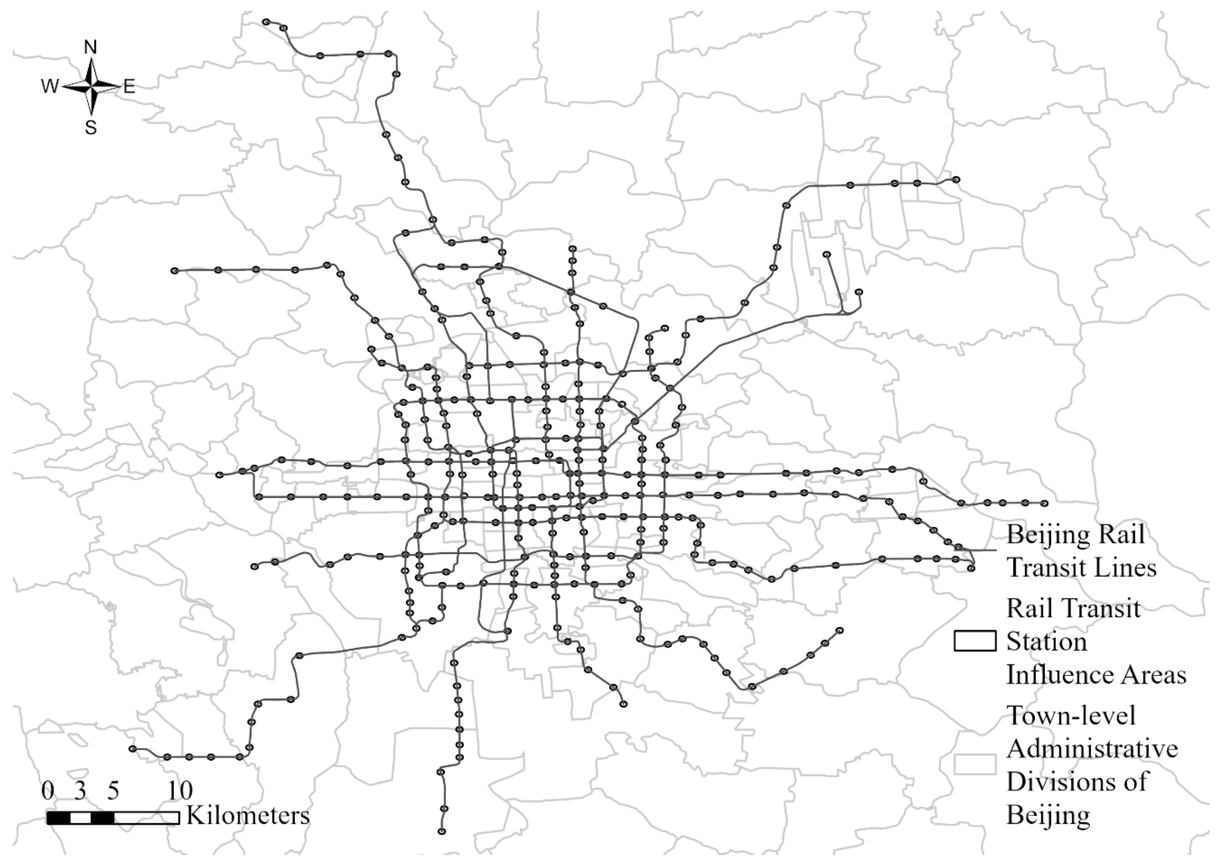
The final non-overlapping influence area radius is determined to be 202 m (Figure 1). All subsequent influence feature calculations are based on this result.

The 202 m radius should be interpreted as a modeling radius derived under the non-overlapping constraint for Beijing’s station density and spatial layout, rather than as a universal walking catchment radius. Compared with the conventional 800 m buffer, it reduces repeated attribution of built-environment and passenger-flow variables in high-density rail corridors. Compared with Voronoi-based delineation, it preserves a station-centered distance logic while avoiding large differences in polygon areas that may bias clustering. However, this value is context-specific and should not be directly generalized to other cities. For cross-city applications, the radius should be recalculated using the same algorithm and tested through sensitivity analysis against local walking-access conditions.

3. Multidimensional Feature Engineering for Station Clustering

Rational feature engineering can significantly improve model performance and is particularly crucial in practical applications. The feature engineering framework in this study comprises three components: feature construction, feature standardization, and feature dimensionality reduction. Features at each scale exhibit distinct measurement units and statistical distributions. By integrating multi-scale data sources, the methodology progressively performs feature standardization and dimensionality reduction to achieve effective feature fusion.

3.1. Feature Construction

Existing studies on station passenger flow clustering typically adopt the following metrics: daily average passenger boarding/alighting volumes, peak-hour passenger flows (morning peak, midday peak, evening peak), and passenger flow kurtosis [37,38,39]. The scale of passenger flow is affected by the transportation function of the station within the rail transit network, its geographic location, and various other factors. These factors result in significant differences in passenger flow between stations with similar functions. In order to portray the impact of spatial heterogeneity of stations on passenger flow, this paper starts from two scenarios of weekdays and weekends, and selects the ratio of the arithmetic mean of the daily highest passenger flow and the daily second-highest passenger flow of the stations to the average hourly inbound passenger flow of the whole network as a measure of the dynamic passenger flow characteristics of the stations. Calculating the above indexes effectively reduces the impact of uneven station passenger flow distribution in different spatial locations. It also allows for a more accurate understanding of the dynamic characteristics of a certain type of station passenger flow within a specific time period, as shown in Equations (2)–(5).

$${\rho }_k^w={\displaystyle \frac{Y_k^w}{Y_k^{\overline{w}}}}$$

(2)

$$Y_k^{\overline{s}}{\rho }_k^s={\displaystyle \frac{Y_k^s}{Y_k^{\overline{s}}}}$$

(3)

$$Y_k^w={\displaystyle \frac{(Y_{k,h_1}^w+Y_{k,h_2}^w)}{2}}$$

(4)

$$Y_k^s={\displaystyle \frac{(Y_{k,h_1}^s+Y_{k,h_2}^s)}{2}}$$

(5)

where ${\rho }_k^w$ and ${\rho }_k^s$ respectively denote the ratio of peak-hour boarding flow to average hourly boarding flow at station $k$ on weekdays and weekends. $Y_k^w$ and $Y_k^s$ represent the peak-hour boarding flow at station k on weekdays and weekends, respectively. $Y_k^{\overline{w}}$ and $Y_k^{\overline{s}}$ correspond to the average hourly boarding flow at station $k$ on weekdays and weekends, respectively. $Y_{k,h_1}^w$, $Y_{k,h_2}^w$, $Y_{k,h_1}^s$ and $Y_{k,h_2}^s$ indicate the highest hourly boarding flow, second-highest hourly boarding flow on weekdays, and highest hourly boarding flow, second-highest hourly boarding flow on weekends at station $k$, respectively.

In the clustering study of rail transit stations, in addition to dynamic passenger flow characteristics, it is essential to comprehensively consider multidimensional influencing factors: (1) Residential attributes should incorporate socio-demographic characteristics such as jobs–housing balance, private car ownership, and education levels; (2) Traffic connection features must account for the proportion of connection modes like bus, bike-sharing, and car; (3) Spatial distribution characteristics should integrate built environment indicators including POI functional density and road network density. These characteristics collectively reveal the coupling mechanisms among station functional heterogeneity, spatial carrying capacity suitability, and user behavior preferences, forming a multi-factor synergistic mechanism. Based on this, this paper establishes a feature set comprising four dimensions: dynamic passenger flow characteristics, resident attributes, accessibility features, and spatial distribution, as specified in

Table 2. Feature selection results.

Type	Feature Name	Definition	ID
Dynamic passenger flow characteristics	Weekdays boarding flow ratio	The ratio of the arithmetic mean of the highest and second-highest weekday passenger flow at station k to the network-wide average hourly boarding passenger flow.	$r_1$
	Weekends boarding flow ratio	The ratio of the arithmetic mean of the highest and second-highest weekend passenger flow at station k to the network-wide average hourly boarding passenger flow.	$r_2$
Resident attributes	Jobs–housing ratio within station influence area	Number of employed residents within the influence area/number of permanent residents within the influence area.	$r_3$
	Car-to-no-car ratio within station influence area	Number of households with private cars within the influence area/number of households without private cars within the influence area.	$r_4$
	Education level within station influence area	Number of residents with a bachelor’s degree or above within the influence area/number of residents below bachelor’s degree level within the influence area.	$r_5$
Accessibility features	Bus connection mode share	Number of passengers transferring by bus/total number of station entries and exits.	$r_6$
	Bike-sharing connection mode share	Number of passengers transferring by bike-sharing/total number of station entries and exits.	$r_7$
	Car connection mode share	Number of passengers transferring by taxi or private car/total number of station entries and exits.	$r_8$
Spatial distribution characteristics	POI density around station	Number of POIs within the influence area/area of the influence area.	$r_9$
	Road network density around station	Total length of roads within the influence area/area of the influence area.	$r_{10}$

.

To improve the clarity and operational definition of the variables studied, this research distinguishes between two groups of variables. The first group consists of clustering variables used for station functional classification, including dynamic passenger-flow characteristics, resident attributes, connection characteristics, and spatial distribution characteristics. The second group consists of explanatory variables used for passenger-flow mechanism analysis. After excluding connection-related variables that may introduce reverse causality, jobs–housing ratio, car-to-no-car ratio, educational attainment ratio, POI density, and road network density are retained, while categorized station passenger flow serves as the dependent variable. All variables are objectively measurable from AFC records, resident attribute data, transfer chains, POI data, and road network data, with definitions and calculation methods summarized in Table 2.

3.2. Feature Standardization

In cluster analysis, algorithms based on spatial distance metrics (e.g., the K-means algorithm) perform sample aggregation by iterating the distance in feature space. However, the presence of multidimensional features with heterogeneous measurement scales may introduce feature weighting bias in Euclidean distance calculations. A typical example is the three-order-of-magnitude disparity between population size (in ten-thousands scale) and connection mode share (percentage scale). Such scale discrepancies can significantly distort clustering outcomes. To mitigate this issue, we implement Min-Max normalization to transform all features into a unified scale, thereby eliminating measurement scale effects. The normalization procedure is as follows:

$$x_{norm}^i={\displaystyle \frac{x_k^i-x_{\min }^i}{x_{\max }^i-x_{\min }^i}}$$

(6)

where $x_{norm}^i$ denotes the standardized value of feature $r_i$ at station $k$, $x_k^i$ represents the original value of feature $r_i$ at station $k$, $x_{\min }^i$ and $x_{\max }^i$ indicate the minimum and maximum values of feature $r_i$ across all stations, respectively.

To preserve variable dispersion and enable equitable comparison of influence strengths on the dependent variable, Z-Score standardization is employed to transform variables into distributions with zero mean and unit standard deviation. This methodological selection demonstrates task-oriented optimization principles. The computational procedure follows:

$$x_{std}^i={\displaystyle \frac{x_k^i-{\mu }_i}{{\sigma }_i}}$$

(7)

where $x_{std}^i$ denotes the standardized value of feature $r_i$ at station $k$, $x_k^i$ represents the original value of feature $r_i$ at station $k$, ${\mu }_i$ and ${\sigma }_i$ indicate the mean value and standard deviation of feature $r_i$ across all stations, respectively.

3.3. Feature Dimensionality Reduction

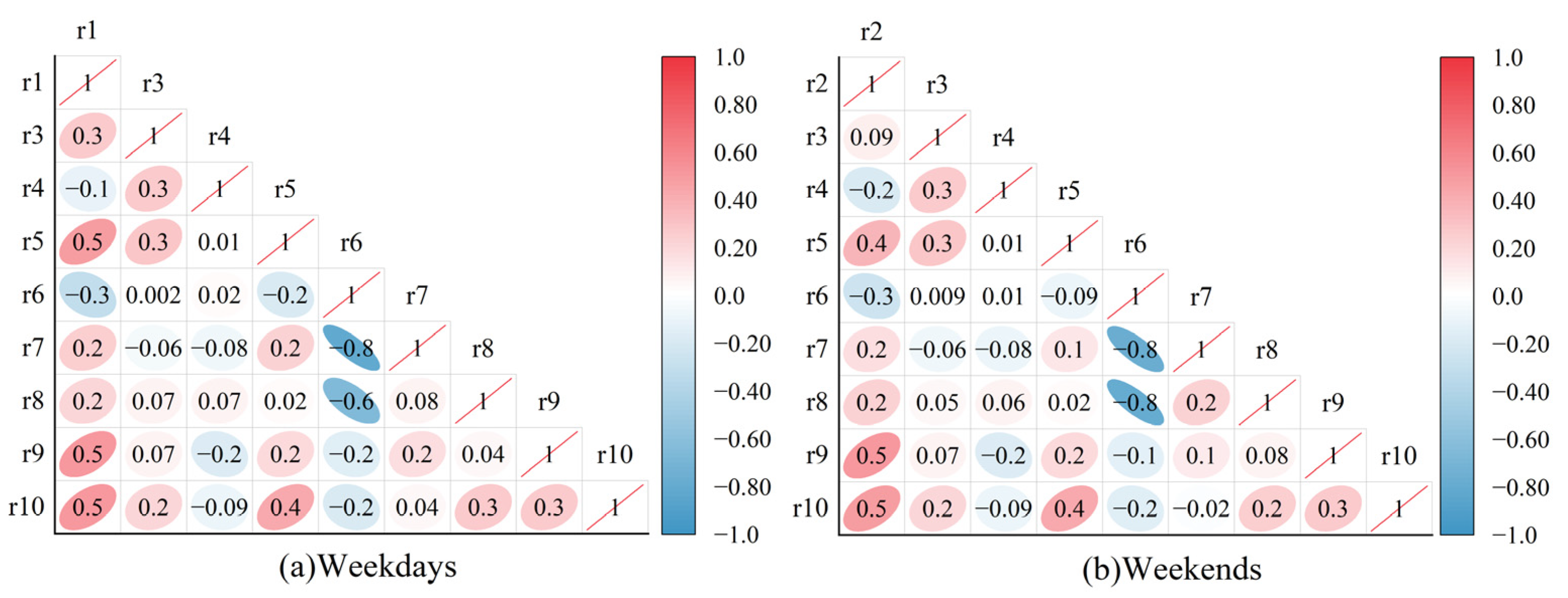
Dimensionality reduction techniques, including feature selection and feature extraction, effectively compress the feature space while preserving critical information. This approach mitigates the negative impacts of the curse of dimensionality while enhancing model generalizability and predictive performance. Accordingly, this paper first conducts correlation analysis using Pearson coefficients, as illustrated in Figure 2. The results demonstrate that for weekdays, bus connection mode share shows high correlation with bike-sharing connection mode share and strong correlation with car connection mode share, while for weekends, bus connection mode share exhibits high correlations with both bike-sharing and car connection mode shares. Consequently, separate dimensionality reduction is essential to reduce data redundancy and improve clustering performance.

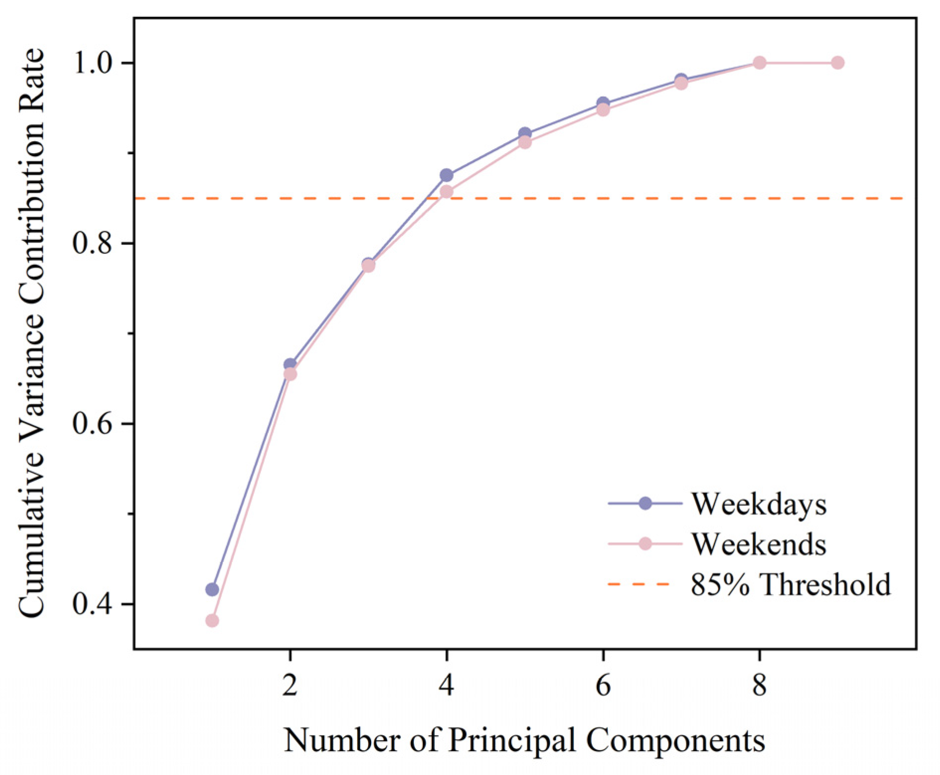
Based on the correlation structure shown in Figure 2, several connection-mode variables exhibit strong correlations. Directly using these variables for clustering may introduce redundancy and distort feature weights. Therefore, Principal Component Analysis (PCA) was further applied to reduce dimensionality while retaining the main information of the original variables. Figure 3 presents the cumulative explained variance after PCA. Since a cumulative explained variance above 85% is generally considered sufficient to preserve the major information of the original data, PCA (n = 4) was selected for both weekday and weekend scenarios.

4. Clustering Algorithms and Regression Models

4.1. PAM Clustering Algorithm with Cosine Distance

4.1.1. Algorithmic Model Construction

This paper employs a PAM (Partitioning Around Medoids) algorithm incorporating cosine distance for clustering, which differs from conventional PAM through its use of cosine distance as the similarity metric. Cosine distance evaluates similarity by measuring directional differences between vectors rather than relying on absolute distance measurements. While PCA preserves the primary variance structure during dimensionality reduction, it alters the scale distribution of the data. Cosine distance demonstrates scale invariance, yielding superior performance on dimensionally reduced data. Furthermore, the PAM algorithm selects medoids directly from existing data points as representative objects, rather than defining centroids through the mean of cluster samples. This approach more accurately reflects the true data distribution and provides more robust clustering results when handling datasets containing noise or outliers. The algorithm was implemented using the scikit-learn-extra library in a Python (v3.13.1) environment, with the random seed set to random_state = 42. The exploration range for the number of clusters was set from K = 3 to K = 10. Model initialization adopted a random selection strategy for medoids, and the iterative process continued until either the objective function converged or the maximum number of iterations was reached. The proposed cosine distance-enhanced PAM algorithm implements the following procedures:

Compared with conventional classification workflows based on fixed-radius buffers and single static indicators, the methodological improvements of this study are threefold. First, non-overlapping influence areas are used instead of fixed buffers to reduce variable mixing caused by overlapping station service areas. Second, passenger-flow, resident, connection, and spatial-environment variables are integrated into a multi-scale feature system, and PCA is applied to reduce redundancy among correlated variables. Third, cosine distance is incorporated into PAM clustering to emphasize directional similarity in station feature structures, while silhouette coefficient, CHI, DBI, Kruskal–Wallis tests, and Dunn post hoc tests are used to validate classification quality. Thus, the proposed method not only assigns station classes but also provides variable-based and statistically testable evidence for class differentiation.

• Cosine Distance Definition

Given feature vectors $X_k=\left(x_{k1},x_{k2},x_{k3},x_{k4}\right)$ and $X_l=\left(x_{l1},x_{l2},x_{l3},x_{l4}\right)$ for stations, where $x_{ki}$ denotes the projection value of station k on the i-th principal component, the cosine distance is computed as:

$$d_{\cos }(X_k,X_l)=1-{\displaystyle \frac{X_k·X_l}{‖X_k‖‖X_l‖}}$$

(8)

where $d_{\cos }\left(X_k,X_l\right)$ represents the cosine distance between station feature vectors $X_k$ and $X_l$, with value range [0, 2], $X_k·X_l$ indicates the dot product of feature vectors, $‖X_k‖$ denotes the L2-norm of vectors.

2.

Objective Function Optimization

The enhanced PAM algorithm minimizes the total cosine distance between all stations and their cluster medoids:

$$\min {\displaystyle \sum _{n=1}^N{\displaystyle \sum _{X_k}{d}_{\cos }(X_k,X_n)}}$$

(9)

where $N$ denotes the number of clusters, $C_n$ represents the $n$-th cluster, and $M_n$ indicates actual sample points within clusters, satisfying:

$$M_n=\arg \underset{X_l\in C_n}{\min }{\displaystyle \sum _{X_k\in C_n}{d}_{\cos }(X_k,X_l)}$$

(10)

3.

Algorithmic Procedure

i.

Initialization: Randomly select N medoids $\left\{M_1,\dots ,\left.M_N\right\}\right.$;

ii.

Assignment Phase: Assign each station $X_k$ to the nearest medoid’s cluster:

$$C_n=\left\{X_k\right.\left|d_{\cos }\right.\left(X_k,M_n\right)\le d_{\cos }\left(X_k,M_{n^{\prime }}\right),\forall n^{\prime }\ne \left.n\right\}$$

(11)

iii.

Update Phase: For each cluster $C_n$, iterate through all samples $X_j\in C_k$ to compute total distances when serving as new medoids, then update with $M_n$ the minimal value;

iv.

Termination Condition: The algorithm terminates when medoids remain unchanged or the maximum iteration count is reached.

4.1.2. Model Evaluation

This paper employs three established metrics—the silhouette coefficient, Calinski–Harabasz Index (CHI), and Davies–Bouldin Index (DBI)—to comprehensively evaluate clustering performance. The mathematical formulations of these indicators are elaborated as follows:

• Silhouette Coefficient

The silhouette coefficient ranges from [−1, 1], with higher values indicating better clustering performance. Its mathematical formulation is expressed as:

$$s={\displaystyle \frac{{\displaystyle {\sum }_{j=1}^K\frac{b_j-a_j}{\max \left\{b_j,a_j\right\}}}}{K}}$$

(12)

where $a_j$ denotes the average distance between sample $X_l$ and all other samples in the same cluster, representing intra-cluster cohesion; $b_j$ indicates the average distance between sample $X_l$ and all samples in the nearest neighboring cluster, representing inter-cluster separation; $s$ represents the mean silhouette coefficient across all samples. Where $S$ denotes the total number of clusters.

2.

Calinski–Harabasz Index

The Calinski–Harabasz Index (CHI) quantifies clustering quality by calculating the ratio between inter-cluster dispersion and intra-cluster dispersion. A higher CHI value reflects superior clustering outcomes. Its mathematical formulation is expressed as:

$$CH={\displaystyle \frac{\frac{B\left(N\right)}{N-1}}{\frac{W\left(N\right)}{K-N}}}$$

(13)

where $B\left(N\right)$ represents the trace of the between-cluster dispersion matrix, quantified as the sum of squared distances between cluster centers and the global centroid weighted by cluster size, reflecting the degree of separation among clusters; $W\left(N\right)$ denotes the trace of the within-cluster dispersion matrix, computed as the sum of squared distances between samples and their respective cluster centers, measuring intra-cluster compactness. Higher CH scores indicate better separation between clusters and greater compactness within clusters.

3.

Davies–Bouldin Index

The Davies–Bouldin Index (DBI) assesses clustering quality by measuring both intra-cluster similarity and inter-cluster dissimilarity through centroid distances. Lower DBI values correspond to improved clustering performance. Its mathematical formulation is defined as:

$$DB={\displaystyle \frac{{\displaystyle \sum _{i=1}^N\underset{j\ne i}{\max }\left(\frac{{\sigma }_i+{\sigma }_j}{d\left(M_i,M_j\right)}\right)}}{N}}$$

(14)

where ${\sigma }_i$ indicates intra-cluster dispersion, calculated as the average distance between points within cluster $i$ and its centroid $M_i$; $d\left(M_i,M_j\right)$ denotes the Euclidean distance between the centroids of clusters $i$ and $j$. Lower DBI values reflect optimal clustering configurations with minimal intra-cluster variance and maximal inter-cluster separation.

4.2. OLS, GWR, and MGWR Models

To systematically analyze the spatial heterogeneity in the influencing mechanisms of station passenger flow, this paper employs a comparative framework incorporating three distinct models: OLS, GWR, and MGWR. The OLS model serves as a global regression benchmark, providing preliminary identification of statistically significant variables. Building upon OLS, the GWR model introduces spatial location parameters, allowing regression coefficients to vary geographically and thereby more accurately capturing localized effects of influencing factors. The MGWR model further extends GWR by permitting distinct spatial smoothing bandwidths for different variables, aligning with real-world scenarios where factors operate at varying spatial scales. Through this progressive comparative approach, the paper aims to identify the optimal spatial scale for each variable, ultimately enabling a more precise revelation of passenger flow influencers and their spatial operational characteristics.

The OLS model estimates parameters in linear regression by minimizing the sum of squared errors, assuming constant coefficients across the study area. The OLS formulation is:

$$Y_k={\beta }_0+{\displaystyle \sum _{r_i}{\beta }_{r_i}}{x}_{std}^i+{\epsilon }_k$$

(15)

where $Y_k$ is the passenger flow at station $k$, ${\beta }_0$ is the intercept, ${\beta }_{r_i}$ are regression coefficients between flow and features, and ${\epsilon }_k$ is the error term at station $k$.

Compared with OLS, GWR provides more nuanced spatial analysis by accommodating spatial heterogeneity. The GWR formulation is:

$$Y_k={\beta }_0\left(u_k,v_k\right)+{\displaystyle \sum _{r_i}{\beta }_{r_i}\left(u_k,v_k\right)}{x}_{std}^i+{\epsilon }_k^{\prime }$$

(16)

where $\left(u_k,v_k\right)$ are coordinates of station $k$, ${\beta }_0\left(u_k,v_k\right)$ is the intercept, ${\beta }_{r_i}\left(u_k,v_k\right)$ are local regression coefficients, ${\epsilon }_k^{\prime }$ is the error term at station $k$.

Compared to the GWR model, the MGWR model allows each explanatory variable to have different bandwidths, reflecting distinct local spatial influence ranges. The MGWR formulation is:

$$Y_k={\beta }_0\left(u_k,v_k\right)+{\displaystyle \sum _{r_i}{\beta }_b\left(u_k,v_k\right)}{x}_{std}^i+{\epsilon }_k^{″}$$

(17)

where ${\beta }_b\left(u_k,v_k\right)$ denotes the regression coefficient of the $r_i$ feature $X_{k{r}_i}$ at station $k$, $b$ represents the optimal bandwidth for this feature’s coefficient, ${\epsilon }_k^{″}$ indicates the error term at station $k$.

This paper employs adjusted R2 and the corrected Akaike Information Criterion (AICc) as metrics for optimal model selection, where models with adjusted R-squared values closer to 1 and smaller AICc values demonstrate superior explanatory power.

5. Case Study

5.1. Station Classification Using Cosine Distance-Based PAM Algorithm

5.1.1. Station Clustering Results

By processing passenger flow data and internal characteristics of influence areas for 326 Beijing rail transit stations, this paper applies the enhanced PAM algorithm to conduct clustering analysis for both weekday and weekend scenarios. To validate its effectiveness, three classical clustering algorithms—K-means, DBSCAN, and conventional PAM—were selected as baseline models. Evaluation was performed using silhouette coefficient, CHI, and DBI and the results are presented in

Table 3. Baseline clustering methods comparison table.

Clustering Algorithm	Weekdays				Weekends
	Optimal Number of Clusters	Silhouette Coefficient	CHI	DBI	Optimal Number of Clusters	Silhouette Coefficient	CHI	DBI
Enhanced PAM	K = 4	0.294	136.033	1.446	K = 3	0.325	160.761	1.210
Classic PAM	K = 5	0.256	124.268	1.331	K = 9	0.270	107.543	1.170
K-means	K = 7	0.287	134.282	1.215	K = 4	0.317	149.940	1.269
DBSCAN	K = 5	0.226	25.222	0.741	K = 2	0.193	19.727	1.004

.

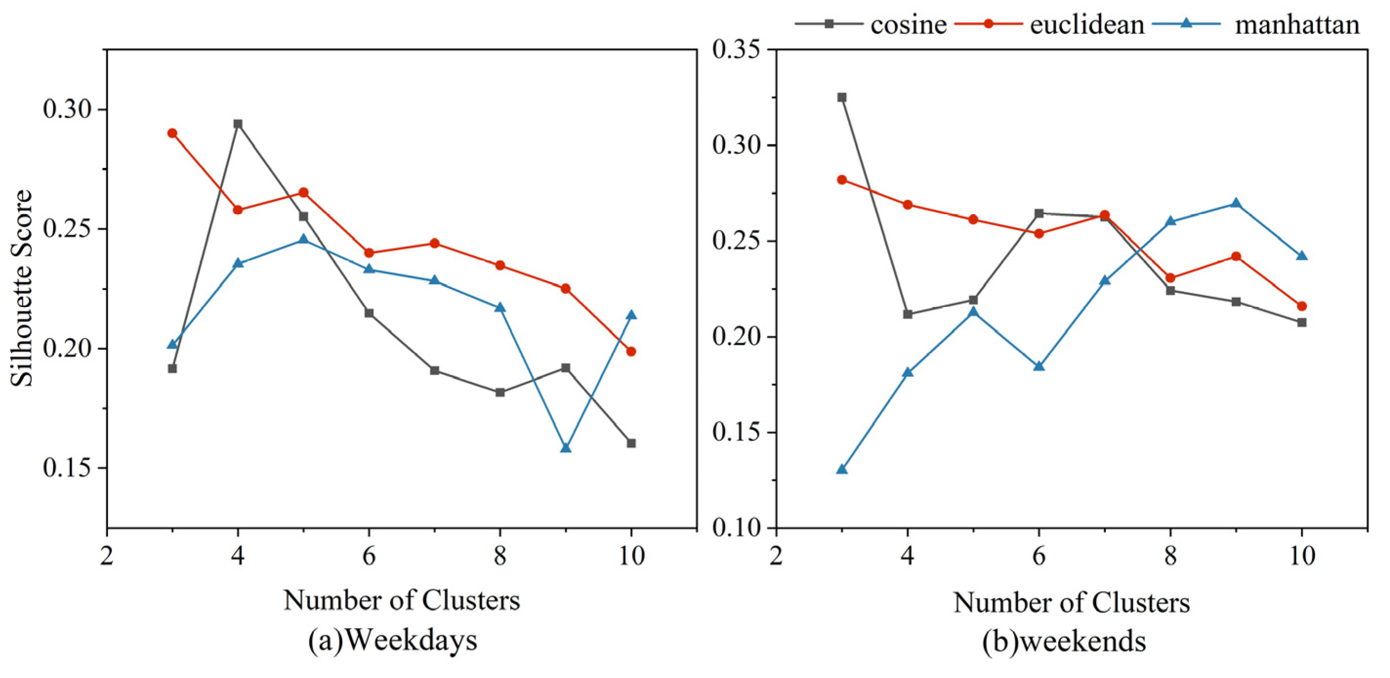
As shown in Table 3, the results comprehensively demonstrate that the enhanced PAM algorithm achieves optimal performance across all metrics. Furthermore, silhouette coefficients were calculated for different cluster numbers under varying distance metrics, with the outcomes visualized in Figure 4.

Results indicate superior performance of the cosine distance-based PAM algorithm compared to Euclidean and Manhattan distances for multidimensional feature clustering, with optimal clustering achieved at K = 4 for weekday and K = 3 for weekend. Consequently, the analysis adopts 4 and 3 clusters respectively, with final clustering results detailed in

Table 4. Cluster classification results.

Temporal Scenarios	Type	Quantity (Units)
Weekday	A	50
	B	88
	C	120
	D	68
Weekend	a	135
	b	115
	c	76

. In Table 4, weekday clusters are labeled A–D, and weekend clusters are labeled a–c to distinguish the two temporal scenarios clearly.

To demonstrate that the above clustering results exhibit significant distinguishability, the Kruskal-Wallis test and Dunn’s post-hoc test were used to verify the differences in the distribution of features among the four categories of weekday sites and the three categories of weekend sites. The test results are shown in

Table 5. Kruskal–Wallis test results by station cluster.

Temporal Scenarios	Feature	H Statistic	p-Value	Significantly Different Category Pairs (p < 0.05)
Weekday	Passenger flow ratio	132.50	<0.001	A–B, A–D, B–C, C–D
Weekday	Jobs–housing ratio	36.51	<0.001	A–B, A–D, B–C, C–D
Weekday	Car-to-no-car status	13.04	0.005	B–C
Weekday	Education level	95.28	<0.001	A–B, A–D, B–C, B–D, C–D
Weekday	Bus connection ratio	218.79	<0.001	A–B, A–C, B–C, B–D, C–D
Weekday	Bike-sharing connection ratio	162.75	<0.001	A–B, A–C, B–C, B–D, C–D
Weekday	Car connection ratio	103.03	<0.001	A–B, A–C, B–C, B–D, C–D
Weekday	POI density	203.75	<0.001	A–B, A–D, B–C, B–D, C–D
Weekday	Road network density	62.36	<0.001	A–B, A–D, B–C, C–D
Weekend	Passenger flow ratio	99.70	<0.001	a–b, a–c, b–c
Weekend	Jobs–housing ratio	18.46	<0.001	a–b
Weekend	Car-to-no-car status	8.87	0.012	a–b
Weekend	Education level	13.27	0.001	b–c
Weekend	Bus connection ratio	186.75	<0.001	a–b, a–c, b–c
Weekend	Bike-sharing connection ratio	121.95	<0.001	a–b, a–c, b–c
Weekend	Car connection ratio	124.98	<0.001	a–b, a–c, b–c
Weekend	POI density	209.93	<0.001	a–b, a–c, b–c
Weekend	Road network density	26.51	<0.001	a–b

. The p-values of the Kruskal-Wallis test for all features across all station categories were less than 0.01. The Dunn post-hoc test further confirmed that significant differences exist between most categories. These results validate the discriminative power of the improved PAM algorithm for classification.

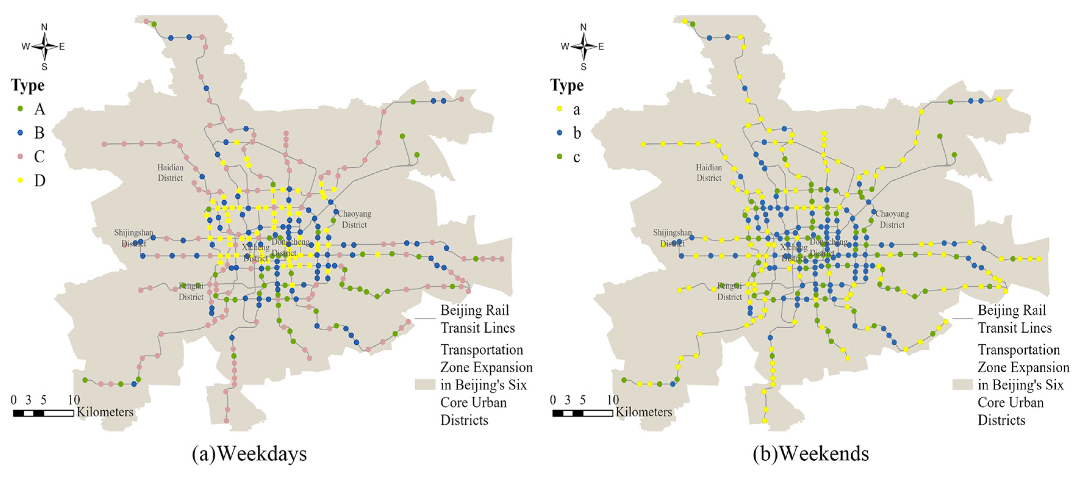
Furthermore, the clustering results were visualized to illustrate the spatial distribution of categorized stations across different temporal scenarios within the urban context, as depicted in Figure 5.

5.1.2. Cluster-Based Analysis of Station Characteristics

• Passenger Flow Characteristic Analysis

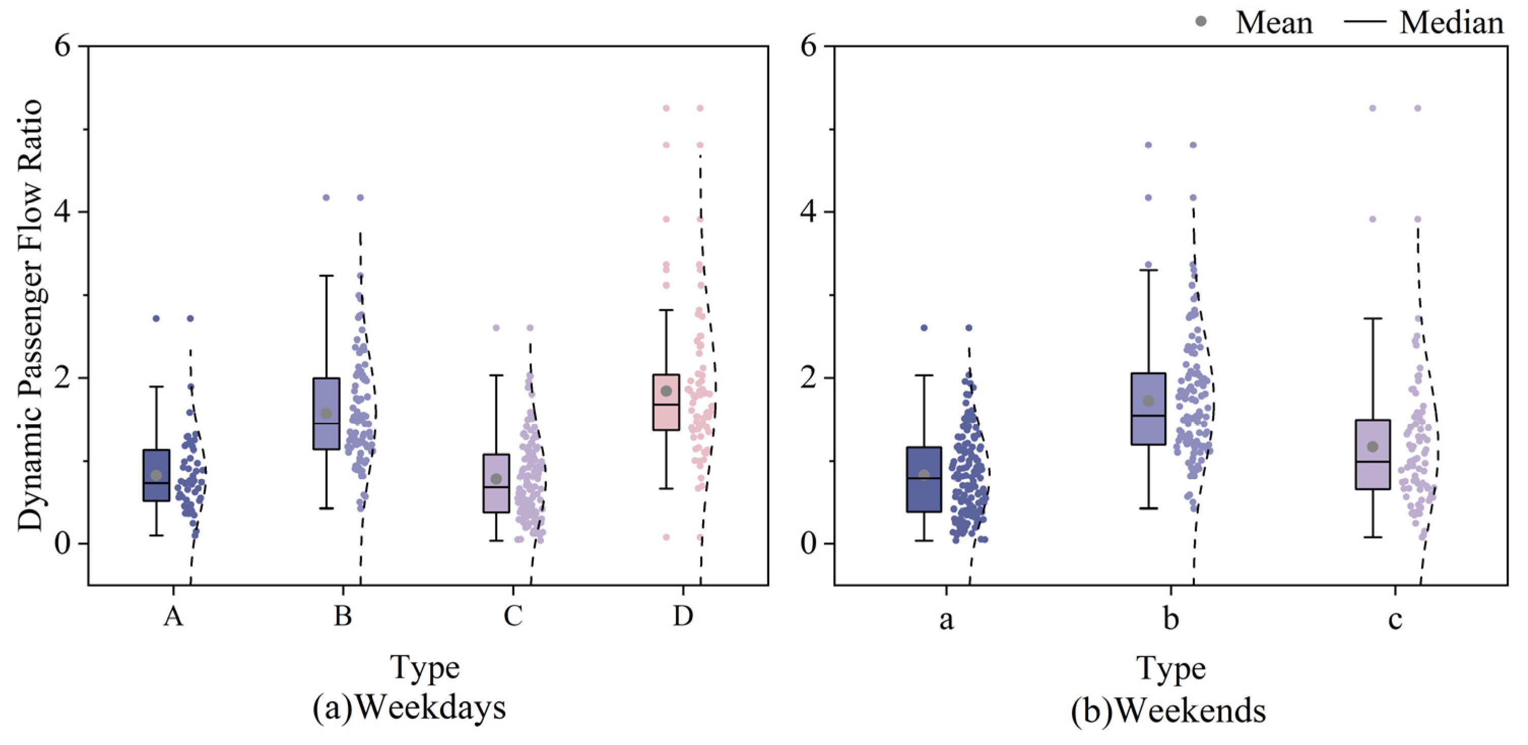
The boxplot analysis in Figure 6 reveals the distribution patterns of station passenger flows and their correlations with spatial functions. On weekdays, Type B and D stations exhibit pronounced peak characteristics (medians: 1.45 and 1.68; means: 1.57 and 1.84), demonstrating commuting-oriented patterns. Type D stations show a Q3 value of 2.04 with marked right-skewness (mean > median), indicating extreme peak flows consistent with transit hubs or central business district (CBD) stations. In contrast, Type A and C stations display balanced distributions (medians: 0.73 and 0.68; means < 0.82), reflecting stable residential-area patterns. For weekend scenarios, Type b stations exhibit strong leisure attributes with Q3 reaching 2.06 and significant right-skewness, aligning with intermittent surge patterns typical of commercial/attraction areas. Type c stations demonstrate notable passenger flow heterogeneity (median: 0.99, mean: 1.17), while Type a stations maintain stable uniformity (median: 0.79, mean: 0.83), consistent with regular weekend travel behavior in residential zones.

2.

Spatial Distribution Pattern Analysis

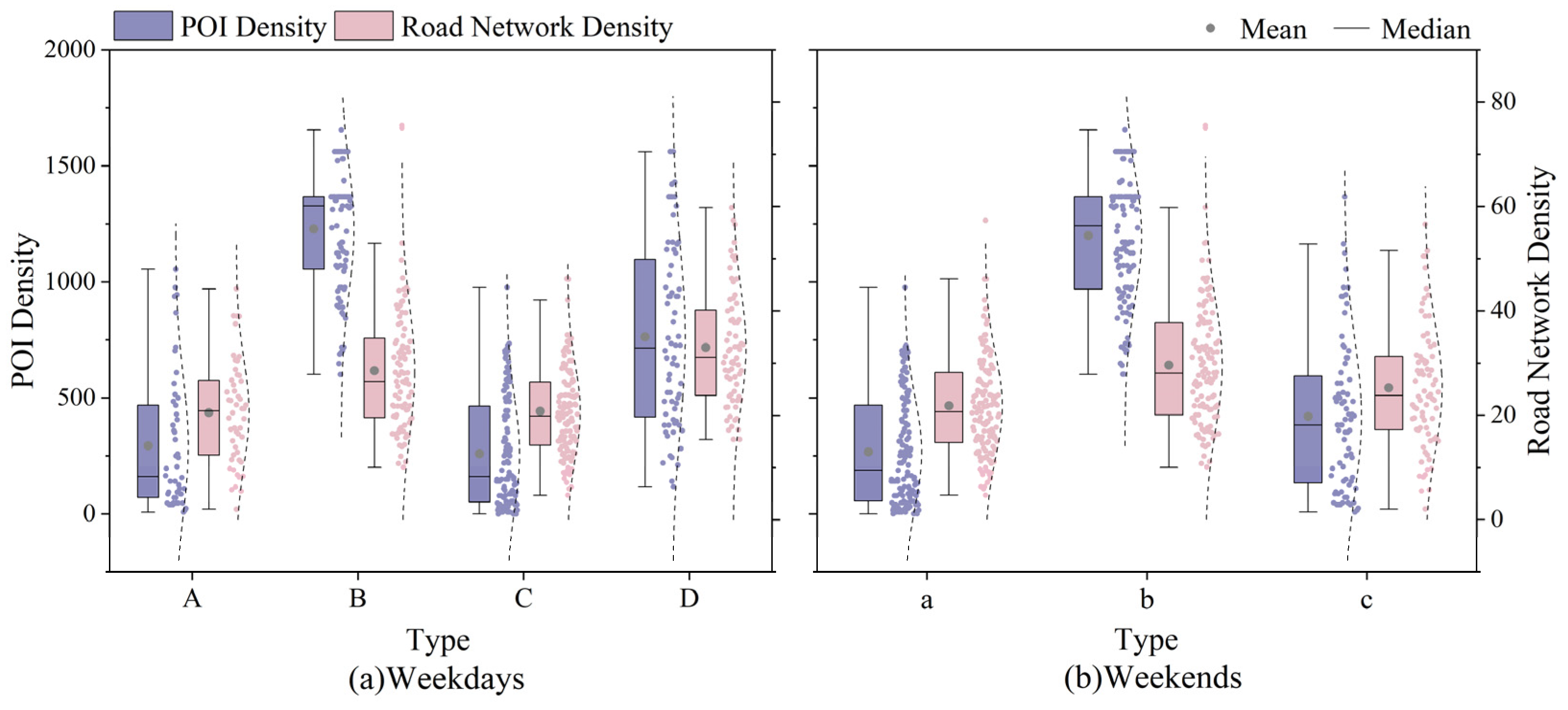
Based on the clustering characteristics, the spatial distribution features of different station types were discussed by combining POI density and road network density indicators, as shown in Figure 7. On weekdays, Type B and D stations function as core commuting hubs, exhibiting significantly higher POI density peaks with concentrated distribution in urban centers. Type D stations demonstrate the highest mean road network density (32.97), corresponding to their peak passenger flow share, highlighting the capacity advantage of high-density central-area road networks for commuting demand. Type B stations show a right-skewed road network density distribution (mean: 28.51, median: 16.45), indicating localized high-density clusters. In contrast, Type A and C stations represent peripheral residential areas, characterized by low POI density and predominant edge-city distribution. Their similar mean road network densities (Type A: 20.52; Type C: 20.76) mask underlying disparities, with Type A’s Q1 as low as 12.36, revealing uneven suburban road network coverage. Weekend scenarios present distinct spatial patterns: Type a stations emerge as edge-dominant residential zones, clustered in urban peripheries with markedly lower mean POI density (266.27). However, their Q3 value (468.37) suggests localized commercial nodes. Type b stations maintain core leisure functions, spatially overlapping with weekday Type B in central areas but showing elevated mean passenger flow (1.72 vs. 1.57 on weekdays), confirming functional transformation from commuting to recreation. Type c stations exhibit hybrid characteristics, with intermediate POI and road network densities (between Types a and b) and transitional spatial distribution, accommodating flexible weekend travel demands.

3.

Connection Mode Characteristics Analysis

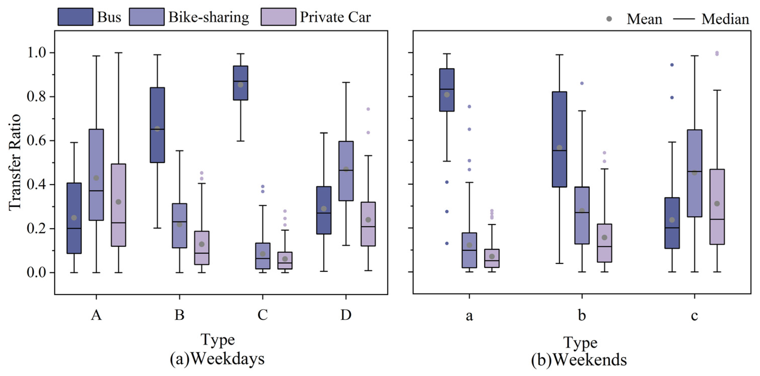
Integrated analysis of bus, bike-sharing, and car connection mode shares reveals distinct patterns across station clusters through quantile analysis (Figure 8). For bus connections, peripheral residential stations (Type C on weekdays/Type a on weekends) exhibit dominant bus dependence (mean shares: 0.85/0.81), with Type C’s Q3 reaching 0.94 (near saturation) while bike-sharing shares remain at only 0.08, highlighting singular bus reliance in fringe areas. Core-area stations (Type B/b) show higher weekday bus shares (mean: 0.65) than weekends (0.57), aligning with their high POI density and right-skewed road network distribution, indicating superior bus efficiency during workdays. Bike-sharing demonstrates complementary roles: central stations (Type D/c) achieve peak shares (mean: 0.47/0.45), leveraging dense road networks and POI concentrations to serve both short-distance transfers and last-mile solutions. Notably, peripheral Type A stations adopt bike-sharing as the primary mode with auxiliary alternatives. Car connections exhibit suppression effects in core areas (Type B/b: mean shares 0.13/0.16), inversely correlating with bus dominance due to parking constraints. Conversely, peripheral Type A stations show the highest car dependence (mean: 0.32), reflecting persistent automobile reliance among suburban commuters despite low-density environments.

4.

Resident Attribute Analysis

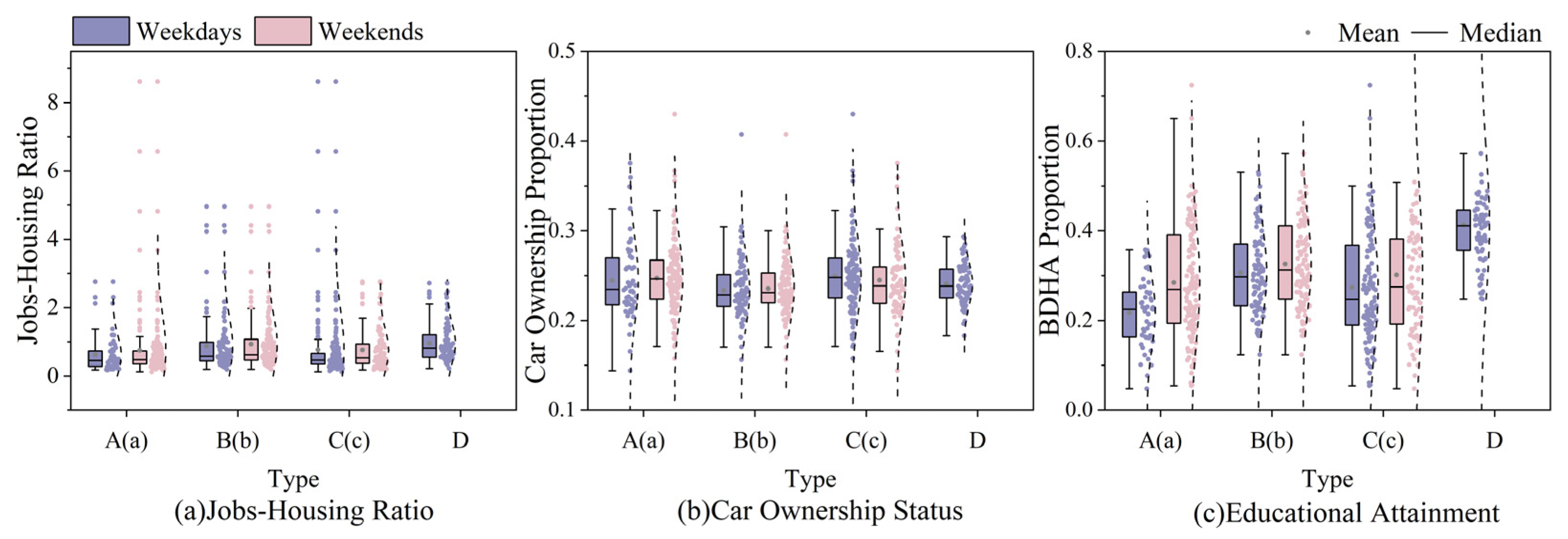
The clustering features of “car-to-no-car ratio” and “educational attainment ratio” are represented by “car ownership proportion” and “bachelor’s degree or higher attainment proportion (abbreviated as BDHA in the figure)”, respectively. Combined with jobs–housing ratio through quantile analysis, this study examines the heterogeneity in resident attributes across cluster groups. The resident characteristics of different station types are illustrated in Figure 9, with detailed distribution metrics of jobs–housing ratio provided in

Table 6. Distribution statistics of job–housing ratio for different categories of stations.

Temporal Scenarios	Type	Mean	Median	Q1	Q3	Proportion of Stations with Jobs–Housing Ratio > 1
Weekday	A	0.62	0.45	0.28	0.73	0.16
	B	0.88	0.58	0.44	0.99	0.23
	C	0.77	0.46	0.35	0.66	0.15
	D	0.96	0.82	0.55	1.2	0.32
Weekend	a	0.75	0.47	0.35	0.73	0.13
	b	0.93	0.62	0.46	1.07	0.29
	c	0.76	0.53	0.37	0.94	0.24

.

The data reveal significant spatial differentiation in resident attributes. The jobs–housing ratio exhibits polarization effects: core-type stations (Type D on weekdays/Type b on weekends) show higher means and greater proportions exceeding 1.0, aligning with their high POI density and commuter flows. Conversely, peripheral residential stations (Type C/a) demonstrate lower ratios with fewer than 15% of stations exceeding 1.0, confirming their residential dominance. Notably, car ownership ratios remain consistently low across all types (mean: 0.23–0.25, SD < 0.02), reflecting strong transit-oriented development (TOD) characteristics. Highly educated clusters (Type D) exhibit slightly lower car ownership (mean: 0.241) than less-educated groups (Type A: 0.244), coupled with higher bike-sharing usage, indicating greener travel preferences. Furthermore, the educated population concentrates more in core areas (Type D/b), demonstrating significantly greater multimodal flexibility compared to less-educated peripheral groups (Type A).

5.1.3. Station Functional Classification

To systematically differentiate the functional characteristics of various station types, this paper integrates the aforementioned feature analyses to establish a comprehensive station classification framework (

Table 7. Functional classification of rail transit stations.

Temporal Scenarios	Type	Comprehensive Characteristics	Core Functions	Designation
Weekday	A	Stable passenger flow, low POI density, bike-sharing dominant, low jobs–housing ratio, low education	Daily mobility guarantee for residential areas	Peripheral Basic-Service Type
	B	High POI density, high bus connection share, jobs–housing imbalance	Commuter service for employment centers	Core Commuting- Aggregation Type
	C	Low POI density, low road network density, near-saturated bus connection share	Rigid commuter accommodation in suburban areas	Exurban Residential- Transit-Dependent Type
	D	Highest road network density, jobs–housing ratio, and educated population	Regional commuter hubs with employment complexes	Multifunctional-Complex Type
Weekend	a	Low passenger flow ratio, low POI density, bus-dependent	Non-compulsory mobility in residential areas	Peripheral Living-Service Type
	b	Coordinated POI density-passenger flow growth, bus-dominant with bike-sharing supplement	Commercial/recreational services in central areas	Core Leisure-Vitality Type
	c	Medium POI density, highly educated population, bike-sharing connection dominant	Cultural-commercial mixed-function accommodation	Central Mixed-Use Type

). The system explicitly defines core functional attributes for each category and ultimately determines their standardized nomenclature, ensuring precise characterization of station roles within the urban transit network.

The naming of station categories is not subjective; rather, it is determined by the combined characteristics of objective indicators, including dynamic passenger-flow peaks, POI density, road network density, connection-mode shares, jobs–housing ratio, and resident attributes. Specifically, a station category is identified as a core commuting, leisure-vitality, or mixed-use type when it simultaneously exhibits relatively high passenger-flow peaks, high POI density, and strong public transport or bike-sharing connection levels. By contrast, categories with low POI density, low road network density, and high bus dependence are identified as peripheral service or exurban residential-dependent types. The preceding Kruskal–Wallis tests and Dunn post hoc tests further demonstrate that the differences among station categories are statistically significant for key variables, indicating that the classification results are both distinguishable and interpretable.

5.2. Analysis of Influencing Variables on Station Passenger Flow

5.2.1. Screening of Significant Influencing Factors on Station Passenger Flow

This paper employs multicollinearity diagnostics to eliminate collinear independent variables [25]. Since connection characteristics fundamentally represent outcome variables rather than causal factors of passenger flow, all connection-related variables were excluded to prevent estimation bias induced by reverse causality in subsequent modeling [40]. Post-collinearity testing revealed that after removing road network density with high variance inflation factor (VIF), the VIF values for “car-to-no-car ratio” and “educational attainment ratio” dropped below 5, though with reduced model R2 indicating the irreplaceable independent contribution of road network density. Consequently, all independent variables except connection features were retained. The OLS stepwise regression was then applied to identify statistically significant influencing features, with the screening results for different station categories presented in

Table 8. Significant feature screening results by station category.

Influencing Feature Variables	VIF	OLS Stepwise Regression Significance Tests
		Weekday Period				Weekend Period
		Peripheral Basic-Service Type (A) p	Core Commuting-Aggregation Type (B) p	Exurban Residential-Transit-Dependent Type (C) p	Multifunctional-Complex Type (D) p	Peripheral Living-Service Type(a) p	Core Leisure-Vitality Type (b) p	Central Mixed-Use Type (c) p
Jobs–housing ratio	2.146	0.002	0.002		0.001	0.004		0.001
Car-to-no-car ratio	5.876	0.015		0.062		0.038		0.011
Educational attainment ratio	5.934	0.007	0.001	0.001	0.013	0.001
POI density	2.715	0.016		0.001		0.001		0.031
Road network density	6.830		0.001	0.007		0.001	0.001	0.002

Note: p denotes significance in OLS stepwise regression; this paper adopts p < 0.1 as the significance threshold.

.

5.2.2. OLS, GWR and MGWR Model Analysis Results

The model fitting results for passenger flow influencing features across different station types are presented in

Table 9. Comparative analysis of model fitting regression results.

Temporal Scenarios	Station Type	Model	R2	Adjusted R2	AICc	Optimal Model
Weekday	Peripheral Basic-Service Type (A)	OLS	0.45	0.40	45.61	OLS
		GWR	0.50	0.41	50.88
	Core Commuting-Aggregation Type (B)	OLS	0.46	0.44	131.76	GWR
		GWR	0.71	0.66	103.10
	Exurban Residential-Transit-Dependent Type (C)	OLS	0.39	0.37	126.75	MGWR
		GWR	0.60	0.53	114.46
		MGWR	0.67	0.60	96.30
	Multifunctional-Complex Type (D)	OLS	0.46	0.45	137.6	GWR
		GWR	0.56	0.51	136.27
Weekend	Peripheral Living-Service Type (a)	OLS	0.43	0.41	201.78	MGWR
		GWR	0.62	0.55	191.27
		MGWR	0.61	0.55	186.44
	Core Leisure-Vitality Type (b)	OLS	0.13	0.12	256.53	GWR
		GWR	0.40	0.32	243.23
		MGWR	0.39	0.31	244.62
	Central Mixed-Use Type (c)	OLS	0.44	0.41	166.24	GWR
		GWR	0.60	0.51	165.28

. Given the limited number of stations in certain categories, MGWR modeling was only applied to categories containing over 100 stations.

For weekday scenarios, the simulation results of peripheral basic-service type stations show that the OLS model yields both a higher adjusted R² and lower AICc value compared to the GWR model. Given their concentrated spatial distribution and limited sample size (with bandwidths of influencing factors approaching the station count of 50), the OLS model demonstrates superior fitting performance due to low spatial heterogeneity. Core commuting-aggregation type stations exhibit better fitting results with the GWR model, evidenced by its higher adjusted R² and lower AICc value relative to OLS. The exurban residential-dependent type stations achieve optimal performance with the MGWR model, which shows the highest adjusted R² and lowest AICc. For multifunctional-complex hubs, the GWR model provides the best fit, maximizing adjusted R² while minimizing AICc.

During weekend periods, peripheral living-service type stations display equivalent adjusted R² values between MGWR and GWR models (both superior to OLS), yet the MGWR model’s lower AICc justifies its selection. Core leisure-vitality type stations show marginal differences between GWR and MGWR models (both outperforming OLS), with MGWR demonstrating slightly better fit. Central mixed-use type stations exhibit optimal results with the GWR model, achieving peak adjusted R² and minimal AICc values.

The model parameter estimates for different station categories are presented in

Table 10. Model parameters estimation results.

Temporal Scenarios	Station Type	Parameter	Influencing Features
			Intercept	Jobs–Housing Ratio	Car-to-No-Car Ratio	Educational Attainment Ratio	POI Density	Road Network Density
Weekday	Peripheral Basic-Service Type (A) (OLS)	$\beta$	1.275	0.312 **	−0.120 **	0.295 **	0.284 **
	Core Commuting-Aggregation Type (B) (GWR)	$\beta$	1.666	0.386 **a		0.334 ***a		0.128 ***
		Bandwidth	52	52		52		52
		Spatial Standard Deviation	0.166	0.224		0.205		0.089
	Exurban Residential-Transit-Dependent Type (C) (MGWR)	$\beta$	1.213		−0.118 *	0.241 ***	0.288 ***a	0.122 **a
		Bandwidth	49		119	116	43	44
		Spatial Standard Deviation	0.118		0.007	0.022	0.108	0.128
	Multifunctional-Complex Type (D) (GWR)	$\beta$	1.861	1.004 ***		−0.138 **
		Bandwidth	60	60		60
		Spatial Standard Deviation	0.052	0.120		0.093
Weekend	Peripheral Living-Service Type (a) (MGWR)	$\beta$	1.615	0.008 **a	−0.153 **	0.195 ***	0.472 ***	0.134 ***a
		Bandwidth	43	88	134	134	134	69
		Spatial Standard Deviation	0.176	0.142	0.019	0.015	0.016	0.120
	Core Leisure-Vitality Type (b) (GWR)	$\beta$	2.202					0.176 ***a
		Bandwidth	46					46
		Spatial Standard Deviation	0.278					0.177
	Central Mixed-Use Type (c) (GWR)	$\beta$	1.817	0.777 ***a	−0.140 **		0.191 **	0.186 **
		Bandwidth	62	62	62		62	62
		Spatial Standard Deviation	0.088	0.245	0.060		0.083	0.075

Note: *, **, *** indicate significance at the 90%, 95%, and 99% levels respectively; $\beta$ parameters represent mean effect coefficients; ^a denotes local variables.

. For weekday scenarios, peripheral basic-service type stations exhibit a negative car-to-no-car ratio effect (a one-unit increase reduces passenger flow by 12%), while jobs–housing ratio, educational attainment ratio, and POI density demonstrate positive impacts (increasing passenger flow by 31.2%, 29.5%, and 28.4% per unit, respectively), indicating that jobs–housing balance effectively reduces rail dependency. Core commuting-aggregation type stations show positive passenger flow associations with jobs–housing ratio and educational attainment ratio (local variables with spatial standard deviations > 0.1) and road network density (global variable), reflecting the combined effects of employment agglomeration, highly educated commuters, and enhanced accessibility from dense road networks. For passenger flow at core commuting-aggregation type stations, the spatial standard deviations of jobs–housing ratio and educational attainment ratio exceed 0.1, classifying them as local variables, while road network density is a global variable. All influencing features show positive effects, ranked by strength as follows: jobs–housing ratio, educational attainment ratio, and road network density. This indicates that high jobs–housing agglomeration attracts commuter flow, concentrated highly educated populations reflect rigid commuting demand, and high-density road networks indirectly promote passenger flow aggregation through enhanced accessibility. Exurban residential-dependent type stations are primarily influenced by educational attainment ratio and POI density (local variables with bandwidths of 43 and 44), with car-to-no-car ratio showing significant negative effects (coefficient: −0.118), confirming private vehicles’ substitution effect on public transit. Multifunctional-complex type stations demonstrate exceptionally strong positive jobs–housing ratio impacts (coefficient: 1.004), highlighting their role as regional employment centers, while educational attainment ratio exhibits negative effects.

During weekends, peripheral living-service type stations maintain negative car-to-no-car ratio effects but positive influences from other factors, with jobs–housing ratio and road network density as local variables. Core leisure-vitality type stations show positive road network density effects (coefficient: 0.176), while central mixed-use type stations reveal strong positive jobs–housing ratio impacts (coefficient: 0.777), emphasizing mixed land-use benefits for weekend passenger flow.

Comparative analysis confirms significant inter-category variations in influential factors and effect magnitudes, though car-to-no-car ratio consistently demonstrates negative effects across all types.

5.2.3. Spatial Impact Analysis of Local Variables on Station Passenger Flow

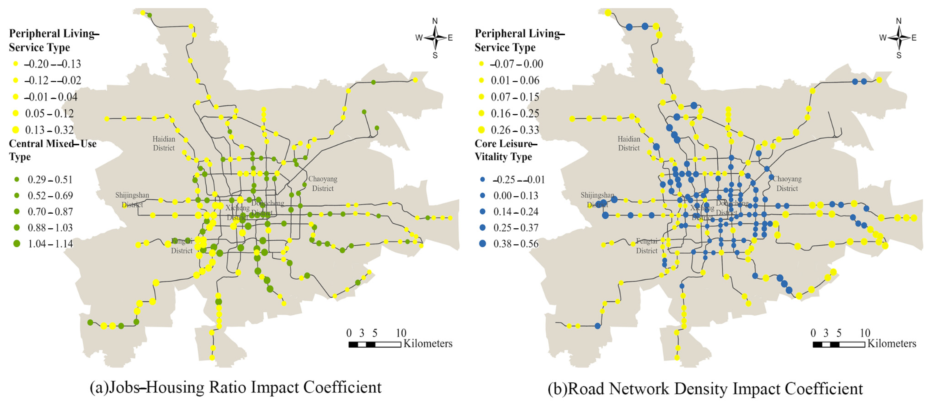
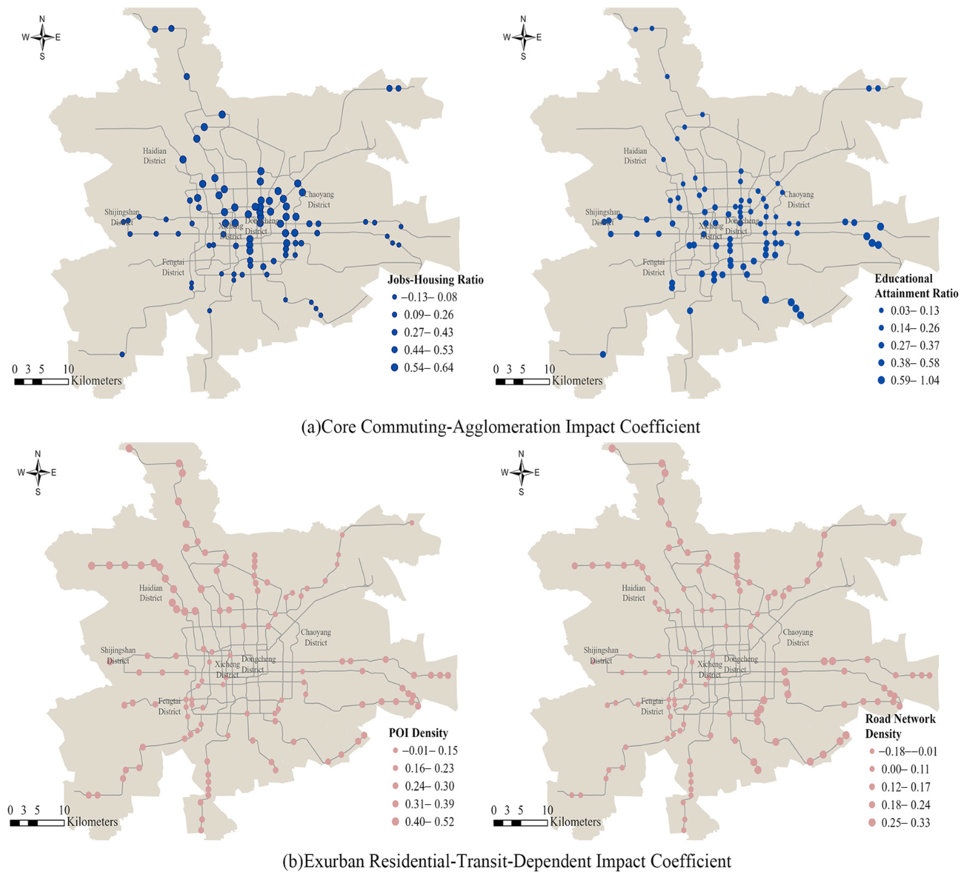
To further investigate the influence of local variables on categorized station passenger flows, spatial analysis was conducted on their effect coefficients using the natural breaks classification method (five levels). The spatial distribution of local variables’ impact intensity demonstrates discernible patterns across different temporal scenarios, as illustrated in Figure 10 and Figure 11.

The analysis reveals significant spatial variations in passenger flow determinants for core commuting-aggregation type stations during weekdays. The jobs–housing ratio coefficients exhibit a decaying pattern from central to peripheral areas, with maximum values observed at key CBD stations like Xizhimen and Zhongguancun—their substantially above-average ratios (3.04–4.40) drive cross-district commuting tides. Conversely, southeastern stations (e.g., Rongchang East Street, Rongjing East Street in Yizhuang) demonstrate negative coefficients due to extreme jobs–housing imbalances, reflecting commuter flow loss caused by unsustainable travel pressures. Educational attainment ratios show an increasing northwest-to-southeast gradient. For exurban residential-dependent type stations, POI density coefficients increase toward urban fringes, where stations like Bei’anhe and Wenyang Road significantly boost passenger flow through multi-purpose trips relying on community-level facilities. Road network density effects peak in northwestern and southeastern sectors, with stations including Nanzhuangzi and Yizhuang Bridge attracting commuters through optimized branch roads and micro-circulation networks that mitigate both jobs–housing mismatches and connection mode limitations.

During weekend periods, the jobs–housing ratio coefficients for peripheral living-service type stations exhibit a decreasing gradient from southwest to northeast, with stations like Guang’anmen Nei and Changchun Street showing the highest values. Conversely, eastern stations including Huazhuang and Tuqiao in Tongzhou demonstrate negative regression coefficients, revealing how low jobs–housing ratios coupled with POI deficiencies diminish rail transit attractiveness. For core leisure-vitality type stations, road network density coefficients increase radially from urban centers, where stations such as Changping and Shahe leverage synergistic effects between high POI density, efficient road networks, and bus connections to drive passenger flows. Central mixed-use type stations display an increasing jobs–housing ratio gradient from northeast to southwest, with stations like Dahongmen and Heyi establishing residential-commercial complementarity through moderate POI and road network densities that attract cross-district travelers despite their low jobs–housing ratios.

Overall, the clustering and regression results indicate that weekday station functions are mainly shaped by commuting intensity, employment concentration, and road-network accessibility, whereas weekend station functions are more strongly associated with leisure-service facilities, mixed-use vitality, and flexible travel demand. Accordingly, weekday management should prioritize tidal-flow organization and feeder-service reliability for core commuting and exurban residential-dependent stations, while weekend management should focus on short-term passenger-flow fluctuations, bike-sharing coordination, and public-space capacity around leisure-vitality and mixed-use stations. These results show that the classification is not merely descriptive, but can be translated into differentiated operational and facility-improvement strategies.

In summary, the jobs–housing ratio, POI density, and road network density emerge as core drivers of passenger flow growth. However, extreme jobs–housing separation (e.g., Yizhuang), deficient road network structures, and low POI density (e.g., peripheral Tongzhou) significantly constrain passenger flow potential.

6. Conclusions

Taking the Beijing urban rail transit system as a case study, this research develops an integrated station functional classification framework that combines non-overlapping station influence areas, enhanced PAM clustering, and spatial regression models. Methodologically, the study shows that non-overlapping influence areas reduce variable mixing between adjacent stations, multi-scale feature fusion captures functional differences more comprehensively, cosine-distance-based PAM clustering improves classification robustness, and MGWR reveals the spatial operating scales of different passenger-flow determinants. Empirically, Beijing rail transit stations are classified into four weekday types, A Peripheral Basic-Service Type, B Core Commuting-Aggregation Type, C Exurban Residential-Transit-Dependent Type, and D Multifunctional-Complex Type, and three weekend types, a Peripheral Living-Service Type, b Core Leisure-Vitality Type, and c Central Mixed-Use Type. Practically, the classification results can support differentiated service planning, feeder bus and bike-sharing integration, station-renewal investment prioritization, passenger-flow management, and TOD function allocation.

The findings of this study provide direct evidence to inform station planning, design, and management: (1) Differentiated strategies should be adopted according to station type. “Core Type” stations require ensuring connectivity within high-density road networks and improving public transport transfer efficiency to cope with tidal passenger flows. “Peripheral Type” stations should focus on compensating for the lack of lifestyle service facilities (POI) and enhancing the accessibility of public services. (2) The analysis of connection characteristics offers strategies for multi-modal transport integration and provides a precise decision-making basis for allocating interchange facility resources across different station categories. (3) The disparity in passenger flow drivers between weekdays and weekends indicates that Transit-Oriented Development (TOD) planning should enhance the integration of “commuting-leisure” functions. Core areas should increase leisure functions to boost weekend vitality, while residential areas should strengthen community services to promote all-day passenger flow balance. In addition, this study has several limitations and directions for future extension. First, the empirical analysis is based only on Beijing, and the applicability of the findings to cities with different urban scales, rail network structures, and travel behavior patterns requires further validation. Second, although this study integrates multi-scale features including dynamic passenger flow, resident attributes, connection characteristics, and spatial distribution, the representation of built-environment factors such as land-use mix, development intensity, population/employment density, and multimodal public transport coupling remains insufficient. Nevertheless, the proposed workflow, including non-overlapping station influence-area delineation, multidimensional feature construction, cosine-distance-based PAM clustering, and comparative OLS/GWR/MGWR analysis, is methodologically replicable. For cities with comparable AFC, POI, road network, resident attribute, and transfer-mode data, this framework can be applied to identify station functional types and examine the spatial heterogeneity of passenger-flow determinants. Future research will expand the analysis to multiple cities and richer data sources to further test the generalizability and robustness of the proposed method.

Based on these findings, station types can be used as basic units for refined rail-transit management. For B and D stations, planning and operation should focus on transfer efficiency, station-area circulation, and peak-flow organization. For C and a stations, priority should be given to feeder bus services, walking/cycling access, and local service facilities. For b and c stations, flexible weekend and holiday capacity, bike-sharing dispatch, and public-space management should be strengthened. This classification-diagnosis-governance chain provides a practical basis for coordination among transport authorities, rail operators, and TOD planners.

References

1. Yang, L.; Chen, Y.; Xu, N.; Zhao, R.; Chau, K.; Hong, S. Place-varying impacts of urban rail transit on property prices in Shenzhen, China: Insights for value capture. Sustain. Cities Soc. 2020, 58, 102140. [Google Scholar] [CrossRef] [Scilit]
2. Yang, L.; Yu, B.; Liang, Y.; Lu, Y.; Li, W. Time-varying and non-linear associations between metro ridership and the built environment. Tunn. Undergr. Space Technol. 2023, 132, 104931. [Google Scholar] [CrossRef] [Scilit]
3. Abdollahpour, S.S.; Le, H.T.K.; Buehler, R.; Hankey, S. Data aggregation impacts on built environment-mode share models around public transit stations. J. Transp. Land Use 2025, 18, 397–424. [Google Scholar] [CrossRef] [Scilit]
4. Cardozo, D.O.; García-Palomares, C.J.; Gutiérrez, J. Application of geographically weighted regression to the direct forecasting of transit ridership at station-level. Appl. Geogr. 2012, 34, 548–558. [Google Scholar] [CrossRef] [Scilit]
5. El-Geneidy, A.; Grimsrud, M.; Wasfi, R.; Tetreault, P.; Surprenant-Legault, J. New evidence on walking distances to transit stops: Identifying redundancies and gaps using variable service areas. Transportation 2014, 41, 193–210. [Google Scholar] [CrossRef] [Scilit]
6. Aud, T.; Marianne, K.; Fitwi, W. Walking distances to public transport in smaller and larger Norwegian cities. Transp. Res. Part D Transp. Environ. 2022, 103, 103169. [Google Scholar] [CrossRef] [Scilit]
7. Huang, Y.; Zhang, Z.; Chen, D.Y. Causality between multi-scale built environment and rail transit ridership in Beijing and Tokyo. Transp. Res. Part D Transp. Environ. 2024, 130, 104150. [Google Scholar] [CrossRef] [Scilit]
8. Li, Z.; Tang, J.; Ji, Y.; Liang, X.; Hu, L.; Hu, C. Relationship between the built environment and metro usage patterns: A motif-based perspective. Tunn. Undergr. Space Technol. 2025, 159, 106488. [Google Scholar] [CrossRef] [Scilit]
9. Li, S.; Lyu, D.; Huang, G.; Zhang, X.; Gao, F.; Chen, Y.; Liu, X. Spatially varying impacts of built environment factors on rail transit ridership at station level: A case study in Guangzhou, China. J. Transp. Geogr. 2020, 82, 102631. [Google Scholar] [CrossRef] [Scilit]
10. Pan, H.; Huang, Y. Tod typology and station area vibrancy: An interpretable machine learning approach. Transp. Res. Part A Policy Pract. 2024, 186, 104150. [Google Scholar] [CrossRef] [Scilit]
11. Tu, W.; Cao, R.; Yue, Y.; Zhou, B.; Li, Q.P.; Li, Q. Spatial variations in urban public ridership derived from GPS trajectories and smart card data. J. Transp. Geogr. 2018, 69, 45–57. [Google Scholar] [CrossRef] [Scilit]
12. Jun, M.J.; Choi, K.; Jeong, J.E.; Kwon, K.H.; Kim, H.J. Land use characteristics of subway catchment areas and their influence on subway ridership in seoul. J. Transp. Geogr. 2015, 48, 30–40. [Google Scholar] [CrossRef] [Scilit]
13. Ding, C.; Cao, X.; Liu, C. How does the station-area built environment influence Metrorail ridership? Using gradient boosting decision trees to identify non-linear thresholds. J. Transp. Geogr. 2019, 77, 70–78. [Google Scholar] [CrossRef] [Scilit]
14. Shao, Q.; Zhang, W.; Cao, X.; Yang, J.; Yin, J. Threshold and moderating effects of land use on metro ridership in Shenzhen: Implications for TOD planning. J. Transp. Geogr. 2020, 89, 102878. [Google Scholar] [CrossRef] [Scilit]
15. Ribeiro, P.; Dias, G.; Pereira, P. Transport Systems and Mobility for Smart Cities. Appl. Syst. Innov. 2021, 4, 61. [Google Scholar] [CrossRef] [Scilit]
16. Degang, D.; Fan, Z. Study on classification of urban rail transit stations from the perspective of land use optimization: A case study on Xi’an subway line 2. City Plan. Rev. 2013, 37, 39–45. [Google Scholar]
17. Papa, E.; Carpentieri, G.; Angiello, G. A TOD classification of metro stations: An application in Naples. Smart Plan. Sustain. Mobil. Age Change 2018, 13, 285–300. [Google Scholar] [CrossRef] [Scilit]
18. Gan, Z.; Yang, M.; Feng, T.; Timmermans, H.J.P. Examining the relationship between built environment and metro ridership at station-to-station level. Transp. Res. Part D Transp. Environ. 2020, 82, 102332. [Google Scholar] [CrossRef] [Scilit]
19. Huang, J.; Chen, S.; Xu, Q.; Chen, Y.; Hu, J. Relationship between built environment characteristics of TOD and subway ridership: A causal inference and regression analysis of the Beijing subway. J. Rail Transp. Plan. Manag. 2022, 24, 100341. [Google Scholar] [CrossRef] [Scilit]
20. Paparrizos, J.; Gravano, L. Fast and accurate time-series clustering. ACM Trans. Database Syst. 2017, 42, 8. [Google Scholar] [CrossRef] [Scilit]
21. Yu, S.; Liu, Y.; Hu, S. Analysis of Spatiotemporal Characteristics of Intercity Travelers Within Urban Agglomeration Based on Trip Chain and K-Prototypes Algorithm. Appl. Syst. Innov. (ASI) 2025, 8, 88. [Google Scholar] [CrossRef] [Scilit]
22. Du, G.; Zhou, L.; Wang, L.; Chen, H. Multivariate time series clustering via multi-relational community detection in networks. Web Big Data 2018, 19, 138–145. [Google Scholar] [CrossRef] [Scilit]
23. Li, H. Multivariate time series clustering based on common principal component analysis. Neurocomputing 2019, 349, 239–247. [Google Scholar] [CrossRef] [Scilit]
24. Zhang, L.; Pei, T.; Meng, B.; Lian, Y.; Jin, Z. Two-phase multivariate time series clustering to classify urban rail transit stations. IEEE Access 2020, 8, 167998–168007. [Google Scholar] [CrossRef] [Scilit]
25. Gu, J.; Jiang, Z.; Fan, W.D.; Wu, J.; Chen, J. Real-time passenger flow anomaly detection considering typical time series clustered characteristics at metro stations. Transp. Res. Part A Policy Pract. 2020, 146, 04020015. [Google Scholar] [CrossRef] [Scilit]
26. Niu, S.; Hu, A.; Shen, Z.; Huang, Y.; Mou, Y. Measuring the built environment of green transit-oriented development: A factor-cluster analysis of rail station areas in Singapore. Front. Archit. Res. 2021, 10, 652–668. [Google Scholar] [CrossRef] [Scilit]
27. Kenger, Ö.N.; Kenger, Z.D.; Özceylan, E.; Mrugalska, B. Clustering of cities based on their smart performances: A comparative approach of fuzzy c-means, k-means, and k-medoids. IEEE Access 2023, 11, 134446–134459. [Google Scholar] [CrossRef] [Scilit]
28. Dong, N.; Li, T.; Liu, T.; Tu, R.; Lin, F.; Liu, H.; Bo, Y. A method for short-term passenger flow prediction in urban rail transit based on deep learning. Multimed. Tools Appl. 2024, 83, 61621–61643. [Google Scholar]
29. Yue, Y.; Chen, J.; Feng, T.; Wang, W.; Wang, C.; Ma, X. New classification scheme and evolution characteristics analysis of high-speed railway stations using large-scale mobile phone data: A case study in Jiangsu, China. J. Transp. Eng. Part A 2023, 149, 12. [Google Scholar] [CrossRef] [Scilit]
30. Bautista-Hernández, D.A. Commuting inequality, role of urban structure, and identification of disadvantaged groups in the Mexico City metropolitan area. J. Transp. Land Use 2020, 13, 159–183. [Google Scholar] [CrossRef] [Scilit]
31. Gao, F.; Yang, L.; Han, C.; Tang, L.; Li, Z. A network-distance-based geographically weighted regression model to examine spatiotemporal effects of station-level built environments on metro ridership. J. Transp. Geogr. 2022, 13, 1706. [Google Scholar] [CrossRef] [Scilit]
32. Zhu, Z.; Zhang, Y.; Qiu, S.; Zhao, Y.; Ma, J.; He, Z. Ridership prediction of urban rail transit stations based on AFC and POI data. J. Transp. Eng. Part A 2023, 149, 04023077. [Google Scholar] [CrossRef] [Scilit]
33. Li, J.; Pan, H.; Liu, W.; Chen, Y. Exploring the relationship between the determinants and the ridership decrease of urban rail transit station during the COVID-19 pandemic incorporating spatial heterogeneity. J. Rail Transp. Plan. Manag. 2024, 32, 100482. [Google Scholar] [CrossRef] [Scilit]
34. Ma, Z.; Yang, X.; Hu, D.; Tan, X. Influence degree analysis of ridership characteristics at urban rail transit stations. J. Tsinghua Univ. (Sci. Technol.) 2023, 63, 1428–1439. [Google Scholar]
35. Zhou, X.; Dong, Q.; Huang, Z.; Yin, G.; Zhou, G.; Liu, Y. The spatially varying effects of built environment characteristics on the integrated usage of dockless bike-sharing and public transport. Sustain. Cities Soc. 2023, 89, 104248. [Google Scholar] [CrossRef] [Scilit]
36. Rong, W.; Zhang, Z.; Liu, Y.; Yang, Y.; Qu, X. Spatiotemporal heterogeneity exploration in the effects of TOD structural characteristics on metro ridership: Evidence from Shanghai. J. Transp. Geogr. 2025, 128, 104339. [Google Scholar] [CrossRef] [Scilit]
37. Wang, Z.; Li, S.; Song, J.; Liu, S.; Liu, D. Contribution of built environment factors and their interactions with subway station ridership. Public Transp. 2024, 16, 929–965. [Google Scholar] [CrossRef] [Scilit]
38. Zhang, J.; Cai, J.; Wang, M.; Zhang, W. An estimation method for passenger flow volumes from and to bus stops based on land use elements: An experimental study. Land 2024, 13, 971. [Google Scholar] [CrossRef] [Scilit]
39. Cui, H.; Ren, Z.; Zhu, M.; Liu, L.; Gao, J. Non-linear impact of built environment on origin–destination passenger flow in Tianjin’s urban rail transit. Proc. Inst. Civ. Eng. Transp. 2025, 179, 76–91. [Google Scholar] [CrossRef] [Scilit]
40. Zhang, B.; Zhou, D.; Du, N.M. Coordination and optimization of long-distance passenger departure timetable connected to high-speed railway station: Considering the heterogeneity of transfer passengers demand. J. Adv. Transp. 2022, 2022, 6743552. [Google Scholar] [CrossRef] [Scilit]
Figure 1. Station influence areas. Source: Authors’ own visualization based on Beijing rail transit station data, Amap/OpenStreetMap road network data, and the datasets described in Section 2.1.
Asi 09 00159 g001
Figure 2. Correlation analysis of feature variables. Source: Authors’ own calculation and visualization based on the datasets described in Section 2.1.
Asi 09 00159 g002
Figure 3. Cumulative explained variance distribution of principal components. Source: Authors’ own calculation and visualization based on the datasets described in Section 2.1.
Asi 09 00159 g003
Figure 4. Clustering performance evaluation. Source: Authors’ own calculation and visualization based on the datasets described in Section 2.1.
Asi 09 00159 g004
Figure 5. Urban spatial distribution of different station categories. Source: Authors’ own visualization based on Beijing rail transit station data, Amap/OpenStreetMap road network data, and the datasets described in Section 2.1.
Asi 09 00159 g005
Figure 6. Dynamic passenger flow characteristics by station category. Source: Authors’ own calculation and visualization based on the datasets described in Section 2.1.
Asi 09 00159 g006
Figure 7. Spatial distribution characteristics by station category. Source: Authors’ own calculation and visualization based on the datasets described in Section 2.1.
Asi 09 00159 g007
Figure 8. Connection features by station type. Source: Authors’ own calculation and visualization based on the datasets described in Section 2.1.
Asi 09 00159 g008
Figure 9. Resident characteristics by station type. Source: Authors’ own calculation and visualization based on the datasets described in Section 2.1.
Asi 09 00159 g009
Figure 10. Spatial distribution of local variable effect coefficients (weekdays). Source: Authors’ own visualization based on Beijing rail transit station data, Amap/OpenStreetMap road network data, and the datasets described in Section 2.1.
Asi 09 00159 g010
Figure 11. Spatial distribution of local variable effect coefficients (weekends). Source: Authors’ own visualization based on Beijing rail transit station data, Amap/OpenStreetMap road network data, and the datasets described in Section 2.1.
Asi 09 00159 g011