UR3 Collaborative Robot Inverse Kinematics Using Metaheuristic Optimization: A Unified Comparative and Experimental Evaluation

Abstract

The inverse kinematics (IK) problem of the UR3 collaborative manipulator is addressed through a singularity-aware optimization framework and a statistically grounded benchmarking methodology. The IK task is formulated as a full-pose optimization problem minimizing a physically scaled residual combining Cartesian position and orientation errors. Emphasizing consistency between error formulation and optimization paradigms, a matrix-based pose-error representation is adopted as a numerically stable residual for stochastic search. Simultaneously, a smooth Jacobian-conditioning penalty is incorporated to mitigate instability near ill-conditioned configurations. Five metaheuristic solvers (PSO, GWO, GA, JADE, ALO) are implemented under a unified, reproducible experimental protocol with common maximum search settings. The Levenberg–Marquardt (LM) numerical method is included as a deterministic baseline to compare gradient-based precision against derivative-free global exploration. Performance is evaluated across nominal, industrial, and near-singular poses using 1000 Monte Carlo runs per configuration. Final-solution accuracy, variability, and computational time are analyzed directly from the Monte Carlo outcome distributions, descriptive statistics, and nonparametric rank-based tests. Results indicate that LM achieves superior numerical precision and computational speed. Among the metaheuristics, GA provides the lowest mean objective values and the smallest objective dispersion across the three tested poses, whereas JADE is the fastest solver. GWO provides an intermediate solution profile, with competitive objective values and substantially shorter execution times than GA and ALO. The optimized solutions are first verified in a RoboDK virtual environment. Subsequently, representative GWO-based configurations are experimentally validated on a physical UR3 robot through both isolated static poses and a continuous multi-pose trajectory tracking task, confirming practical kinematic feasibility and sequential stability. The proposed framework establishes a reproducible benchmark for statistically robust evaluation of metaheuristic-based IK optimization in collaborative robotics.

1. Introduction

For robot manipulators, the solution to the inverse kinematics (IK) problem is defined as the process of determining a joint configuration that achieves a desired end-effector pose. Although several 6-Degree-of-Freedom (DoF) manipulators allow closed-form solutions, these expressions often become difficult to evaluate in practice due to numerical sensitivity, multi-solution branches, and the geometric coupling between axes. These limitations are particularly evident when the manipulator operates near singular configurations, where the Jacobian matrix becomes ill-conditioned and solution stability degrades [1]. Similar findings have been reported for continuum and redundant robots, further emphasizing the need for robust numerical techniques [2,3].

Classical numerical approaches, such as Jacobian inversion, pseudoinverse methods, and Newton-based schemes, depend strongly on differentiability and well-conditioned matrices. Their performance deteriorates significantly near singularities or in multimodal regions of the configuration space [4,5]. Studies on adaptive mutation and differential evolution for IK highlight that iterative methods may converge to suboptimal solutions if the initial estimate is not sufficiently close to the feasible set [6,7]. Additional numerical analyses indicate that local-search schemes remain vulnerable to degeneracies in the Jacobian structure, limiting their applicability in sequences of rapidly changing poses [8,9].

Most of the IK literature focuses solely on Cartesian position $(x,y,z)$ while simplifying the orientation representation. These models are suitable when the task allows moderate rotational deviations or when system requirements prioritize positional convergence. Several works indicate that position-only IK solutions can be acceptable when translational errors are small; however, the authors of [10] do not define a universal numeric threshold. Moreover, acceptable error levels depend on the task and robot (e.g., surgical vs. industrial) and should be justified depending on the robot application. Other studies using neural estimators similarly suggest that orientation can be relaxed in low-precision scenarios [11,12]. Nevertheless, for welding, inspection, assembly, or painting, the orientation constraint is essential and cannot be decoupled from the translational objective [13].

To address the weaknesses of analytical and iterative numerical methods, population-based metaheuristics have gained relevance in robotics. These solvers are derivative-free, operate effectively in nonconvex landscapes, and maintain performance near singularities due to their global search behavior [14,15]. Hybrid Particle Swarm Optimization (PSO)-Grey Wolf Optimizer (GWO) methods have shown improved exploration–exploitation balance in high-dimensional spaces relevant to robotic systems [16]. Likewise, variants of GWO equipped with adaptive learning mechanisms have demonstrated faster convergence while preserving stability in noisy or multimodal environments [17].

Recent work on randomness-enhanced GWO formulations indicates performance improvements in accuracy and convergence for IK problems involving redundancy [18,19,20]. Multi-strategy GWO approaches have also demonstrated competitive performance for general engineering optimization, underscoring their suitability for robotic models with strong nonlinearities [21,22]. Complementary research on PSO highlights its versatility for controller tuning and trajectory design in noisy or mixed-discrete settings [23]. Efforts to improve PSO efficiency through optimal computing budget allocation further support its use in stochastic robotic environments [24,25,26].

Metaheuristics outside the wolf and swarm based families also contribute to IK optimization. The Ant Lion Optimizer (ALO) has shown utility in trajectory tracking and obstacle avoidance for redundant manipulators [27]. Evolutionary–neural hybrid strategies demonstrate that Artificial Neural Network (ANN) models can provide better initial estimates while metaheuristics refine the full-pose solution, yielding improved convergence speed for agricultural and Selective Compliant Assembly Robot Arm (SCARA) manipulators [28]. Other hybrid formulations extend these findings to additional robotic configurations, expanding the design space of metaheuristic-assisted IK solution schemes [29,30,31].

Further contributions include improved trajectory planning for redundant manipulators using GWO variants with enhanced search operators [25,32,33]. Studies employing DE (Differential Evolution)-CCD (Cyclic Coordinate Descent) hybrids provide evidence that combining evolutionary exploration with local correction can improve IK robustness in manipulators with strong joint coupling [34,35]. Penalization of near-singular poses through Jacobian-based indicators has also proven beneficial, helping avoid unstable configurations during optimization [36]. These findings collectively highlight the need for IK formulations that integrate full-pose accuracy, explicit singularity handling, and robustness against nonconvexity.

Herein, a formulation of the IK problem as a minimization of a physically scaled pose error combining translation and rotation on the UR3 collaborative manipulator is presented. The formulation incorporates a singularity-aware penalization strategy derived from Jacobian conditioning, enabling the optimizer to avoid near-degenerate configurations. This approach maintains compatibility with industrial precision requirements while acknowledging that some operational tasks may tolerate translational deviations on the order of a few centimeters.

Five population-based metaheuristics (PSO, GWO, GA, JADE, and ALO) are implemented under a unified experimental protocol to guarantee methodological consistency and fair comparison. Each algorithm is evaluated in terms of accuracy, variability, runtime, and convergence behavior across representative task-space configurations, including nominal poses, industrial orientations, and near-singular arrangements. This unified approach responds to a recurrent gap in the literature, where IK studies frequently evaluate a single algorithm without a clear justification for its selection or without systematic criteria supporting its superiority over alternative solvers.

The research gap addressed in this work is, therefore, methodological rather than merely algorithmic. Existing metaheuristic-based IK studies commonly report successful convergence for a specific solver or a limited set of target poses, but they rarely combine all five elements in a single framework: full-pose residual formulation, explicit singularity avoidance through Jacobian conditioning, deterministic baseline comparison, large-scale Monte Carlo evaluation, and virtual/physical feasibility verification. As a result, the literature still lacks a controlled benchmark that enables comparison of the accuracy, repeatability, runtime behavior, and practical executability of different zero-order solvers under common maximum-search settings.

The novelty of the proposed framework lies in this integrated evaluation protocol. Instead of proposing a new metaheuristic variant, the study establishes a reproducible IK benchmarking methodology for collaborative manipulators. The framework links a matrix-based full-pose residual, a smooth singularity-avoidance fitness, common computational settings, rank-based statistical assessment, RoboDK verification, and physical UR3 execution. This combination provides a clearer basis for selecting a solver according to the task’s engineering requirements, such as accuracy, repeatability, execution time, or robustness near ill-conditioned poses.

To further contextualize the present contribution within recent developments in metaheuristic-based inverse kinematics optimization,

Table 1. Methodological comparison of recent metaheuristic-based inverse kinematics studies.

Reference	Robot/Platform	Metaheuristic Approach	Singularity-Aware Treatment	Statistical Evaluation	Physical Validation	Benchmark Scope
El Mrabet et al. (2025) [37]	ABB IRB1600	ACO, MOA, ALO	N.R.	N.R.	No	Single-study platform
Chen et al. (2025) [38]	6-DoF industrial arm	Improved COA	Modified D–H modeling	N.R.	No	Single-study platform
Duymazlar et al. (2023) [39]	ABB IRB120	Boomerang Swarm Optimization	N.R.	N.R.	No	Single-study platform
Li et al. (2026) [40]	6-DoF collaborative robot	Improved PSO	N.R.	Limited statistical evaluation	Yes	Single-study platform
This work	UR3 collaborative robot	PSO, GWO, GA, JADE, ALO + LM	Smooth Jacobian-conditioning penalty	1000 independent runs per method	Yes	Unified benchmark under the same robot, task, objective function, and validation protocol

Note: N.R. = not reported in the corresponding cited study. The table provides a methodological comparison and is not intended to rank algorithmic performance across heterogeneous robotic platforms.

presents a methodological comparison of representative studies. Since these works involve different robotic platforms, task conditions, objective functions, and validation protocols, the table is not intended to provide a direct performance ranking across algorithms. Instead, it identifies methodological elements that are central to reproducible inverse kinematics evaluation, including singularity-aware treatment, statistical robustness, physical validation, and unified benchmarking conditions.

The table deliberately includes a broad spectrum of recently applied metaheuristic approaches, such as ACO, MOA, and Boomerang Swarm Optimization, to reflect the diversity of current research in this field. However, the comparison is focused on methodological rigor rather than algorithmic superiority. As shown in Table 1, regardless of the specific metaheuristic variant employed, several recent studies do not report standardized computational budgets, large-scale statistical validation, explicit singularity-handling mechanisms, or controlled experimental benchmarks.

In this context, the proposed framework addresses these gaps by evaluating multiple solvers under identical experimental conditions. Specifically, PSO, GWO, GA, JADE, and ALO are compared using the same UR3 inverse kinematics formulation, objective function, constraints, computational budget, and validation protocol. In addition, the framework incorporates an explicit Jacobian-conditioning penalty and performs extensive statistical evaluation through 1000 independent runs per method, followed by validation in both a RoboDK digital twin and a physical UR3 robot.

The primary contribution of this work is the development of a rigorous and reproducible benchmarking framework for inverse-kinematics optimization in collaborative robotic manipulators. In addition to evaluating five population-based metaheuristic solvers under common maximum computational settings, the study incorporates the well-established deterministic Levenberg–Marquardt (LM) algorithm as a reference baseline. As an industry-standard method for differential kinematics, LM enables a principled comparison between gradient-based local convergence and the global exploration capabilities of stochastic population-based methods. This dual deterministic–stochastic assessment provides a structured quantification of the trade-offs between computational efficiency, numerical precision, and probabilistic robustness.

Beyond algorithmic comparison, the study introduces a standardized evaluation methodology grounded on large-scale Monte Carlo experimentation and rank-based statistical assessment. Each solver is assessed under the same maximum population size, iteration limit, joint bounds, and stopping rule. The comparative interpretation is intentionally based on the reported table values and statistical ranks rather than on a single weighted aggregate score. This avoids imposing subjective priorities among accuracy, stability, and runtime and allows readers to select a solver based on the requirements of a specific robotic task.

It is important to clarify the scope and operational context of this comparative study. Deterministic gradient-based methods, particularly the LM algorithm, remain the undisputed gold standard for solving the inverse kinematics of rigid, non-redundant 6-DoF manipulators operating in standard, obstacle-free environments. Therefore, the primary objective of evaluating metaheuristic approaches is not to replace LM in these well-modeled scenarios. Instead, this study utilizes the standard UR3 manipulator purely as a geometrically exact, controlled benchmark testbed. Thus, the UR3 is used as a controlled testbed to evaluate the kinematic feasibility, convergence behavior, and trajectory-tracking stability of zero-order solvers under reproducible conditions.

Finally, the proposed framework extends beyond numerical validation. All optimized joint configurations are verified in simulation using a RoboDK virtual environment (benchmarked in [41]). Furthermore, to bridge the gap between static optimization metrics and real-world operational requirements, representative GWO-based solutions are experimentally deployed on a physical UR3 collaborative robot. This physical validation encompasses both point-to-point convergence and a sequential multi-pose trajectory task. This dual validation demonstrates that the reported optimization results are not only mathematically consistent but also physically implementable in realistic cobotic operation scenarios, where pose fidelity, kinematic stability, and sequential repeatability are critical.

2. Robot Kinematic Models

In the field of robotics, two fundamental kinematic models are used to describe and control robot motion: Forward and Inverse Kinematics. The properties of these models are fundamentally determined by the relationship between the number of joint variables, n, and the number of Cartesian coordinates required to specify the End-Effector (EE) pose, m. When the number of joints equals the task-space DoF ($n=m$), the robot is considered non-redundant. If, however, the robot has more DoF than are strictly necessary for its task ($n>m$), it is classified as a redundant robot. This redundancy provides additional dexterity that can be exploited to optimize trajectories, navigate around obstacles, or avoid kinematic singularities.

2.1. Forward Kinematics

The first model is the FK model, which maps the robot’s joint positions to its EE pose (position and orientation) in Cartesian space. This relationship is defined by the following equation:

$$X=f\left(q\right)$$

(1)

Here, $q\in {\mathbb{R}}^{n\times 1}$ represents the vector of joint variables, and $X\in {\mathbb{R}}^{m\times 1}$ denotes the robot’s Cartesian coordinates. The function $f\left(q\right)$ is a nonlinear mapping that translates the joint configuration into a specific EE pose.

2.2. Inverse Kinematics

Conversely, the IK model performs the opposite operation. It computes the required joint variables to achieve a desired EE pose. This is represented by the inverse mapping:

$$q=f^{-1}\left(X\right)$$

(2)

This model is critical for tasks where the robot must reach a specific location or pose in Cartesian space, as it provides the necessary joint angles to achieve that goal.

2.3. Velocity Kinematics and the Jacobian

Beyond static position, it is also crucial to relate joint velocities to end-effector velocities. The relationship between the Cartesian velocity $\dot{X}\in {\mathbb{R}}^{m\times 1}$ and the joint velocity $\dot{q}\in {\mathbb{R}}^{n\times 1}$ is linear and is governed by the robot Jacobian matrix. This is given by the following equation:

$$\dot{X}=J\left(q\right)\dot{q}$$

(3)

In this expression, $J\left(q\right)={\displaystyle \frac{\partial f\left(q\right)}{\partial q}}\in {\mathbb{R}}^{m\times n}$ is the Jacobian matrix, which is a function of the joint configuration. The Jacobian serves as a local velocity transformation matrix, linking velocities from the joint space to the Cartesian space. It is essential for various applications, including trajectory planning and singularity analysis.

2.4. Kinematic Singularities

A kinematic singularity is a configuration of a robot manipulator where the robot loses one or more DoF of motion. At such a point, the manipulator’s end-effector is unable to move in certain directions, regardless of the joint velocities. These configurations are problematic because they can lead to unpredictable behavior, and the inverse kinematics solution becomes non-unique or ill-conditioned, potentially requiring infinite joint velocities to achieve a finite Cartesian velocity.

Singularities are directly related to the rank of the Jacobian robot matrix, $J\left(q\right)$. A singularity occurs when the Jacobian matrix becomes rank-deficient, meaning its rank is less than the maximum possible value.

For a square Jacobian matrix (i.e., for non-redundant robots ($n=m$)), a singularity exists when the determinant of the Jacobian is zero:

$$det\left(J\left(q\right)\right)=0$$

(4)

For a non-square Jacobian, where the number of rows m does not equal the number of columns n, the determinant is not defined. In this more general case, a singularity is identified when the rank of the Jacobian is less than its number of rows:

$$rank\left(J\left(q\right)\right)<m$$

(5)

This condition indicates that the transformation from joint velocities to Cartesian velocities is not invertible. Analyzing the Jacobian to identify singular configurations is a critical step in robot design and trajectory planning to ensure the robot operates within its dexterous workspace.

3. UR3 Kinematics and Objective Functions

In contemporary robotics, the focus has shifted beyond single-robot applications to embrace solutions where humans and machines can collaborate effectively. This paradigm is driven by the emergence of collaborative robots or cobots, which have become a pivotal tool for automating a wide range of tasks. As highlighted by Universal Robots (UR) [42], cobots are designed to operate safely in a shared workspace with human operators, thereby simplifying automation and expanding its accessibility across diverse industrial and service-oriented applications. In this section, the UR3 robot main features and models are used to define the objective functions to be used in the optimization problem.

3.1. UR3 Robot Features

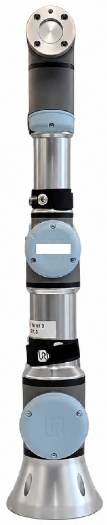
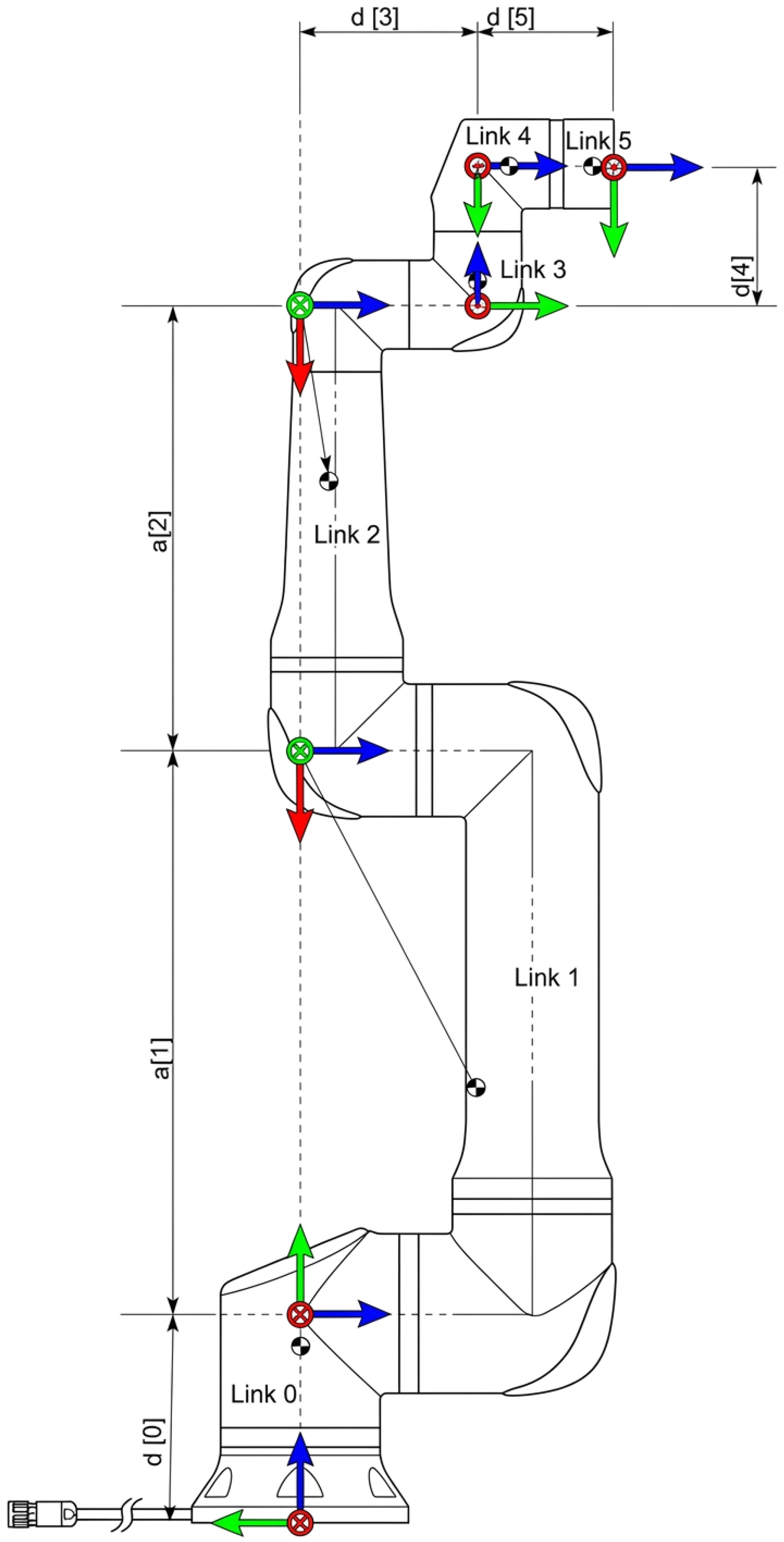
The UR3 robot is a notable example of this technology, serving as a key mechanism for collaborative tasks. Its primary features include six revolute joints, which provide 6-DoF for high maneuverability, a reach of 500 mm (19.7 in), and a payload capacity of 3 kg. The manipulator’s high repeatability of ± 0.1 mm (± 0.0039 in) ensures consistent performance. Its control is facilitated by the PolyScope software, developed by UR, which provides a comprehensive interface for configuring, moving, and controlling the robot via a 12-inch touchscreen Teach Pendant. The robot’s physical structure is illustrated in Figure 1, and its movement parameters are detailed in

Table 2. UR3 Denavit–Hartenberg parameters used in this study.

i	${\mathit{a}}_{\mathit{i}}$ (m)	${\mathit{\alpha }}_{\mathit{i}}$ (rad)	${\mathit{d}}_{\mathit{i}}$ (m)	${\mathit{\theta }}_{\mathit{i}}$	Joint
1	0	$\pi /2$	0.1519	$q_1$	R
2	$-0.24365$	0	0	$q_2$	R
3	$-0.21325$	0	0	$q_3$	R
4	0	$\pi /2$	0.11235	$q_4$	R
5	0	$-\pi /2$	0.08535	$q_5$	R
6	0	0	0.0819	$q_6$	R

.

3.2. Forward Kinematics

To develop a precise mathematical model of the robot’s kinematics, this work utilizes the Standard (Classic) Denavit–Hartenberg (D-H) convention [43]. The forward kinematics of the UR3 manipulator were computed using a custom MATLAB script, relying on the official kinematic specifications provided by Universal Robots in [44]. Figure 2 illustrates the standard D-H coordinate frame assignments for the UR3. It is important to note that the negative values for the link lengths $a_2$ and $a_3$ strictly follow the manufacturer’s official kinematic orientation. These negative values arise because the intermediate x-axes (red arrows) point in the opposite direction of the physical link extension in order to maintain a consistent right-hand rule configuration across the parallel z-axes. Table 2 outlines the standard D-H parameters used in this analysis.

Let $q={[q_1,\dots ,q_6]}^{\top }$ denote the joint configuration. The homogeneous transformation from the base to the end-effector is computed as:

$${\mathbf{T}}_{06}\left(q\right)={\displaystyle \prod _{i=1}^6}{\mathbf{A}}_i\left(q_i\right),{\mathbf{A}}_i\left(q_i\right)=\left[\begin{array}{cccc}cos{q}_i& -sin{q}_{i}cos{\alpha }_i& sin{q}_{i}sin{\alpha }_i& a_{i}cos{q}_i\\ sin{q}_i& cos{q}_{i}cos{\alpha }_i& -cos{q}_{i}sin{\alpha }_i& a_{i}sin{q}_i\\ 0& sin{\alpha }_i& cos{\alpha }_i& d_i\\ 0& 0& 0& 1\end{array}\right],$$

(6)

with ${\theta }_i=q_i$ for revolute joints. The end-effector position and rotation matrix are $\mathbf{p}\left(q\right)={\mathbf{T}}_{06}(1:3,4)$ and $\mathbf{R}\left(q\right)={\mathbf{T}}_{06}(1:3,1:3)$, respectively.

3.3. Jacobian

The geometric Jacobian $\mathbf{J}\left(q\right)\in {\mathbb{R}}^{6\times 6}$ is obtained from the intermediate homogeneous transforms ${\mathbf{T}}_{0k}$$(k=1,\dots ,6)$, where ${\mathbf{o}}_k$ is the origin of frame k and ${\mathbf{z}}_k$ is its z axis, both expressed in the base frame:

$$\mathbf{J}\left(q\right)=\left[\begin{array}{cccc}{\mathbf{z}}_0\times ({\mathbf{o}}_6-{\mathbf{o}}_0)& {\mathbf{z}}_1\times ({\mathbf{o}}_6-{\mathbf{o}}_1)& \dots & {\mathbf{z}}_5\times ({\mathbf{o}}_6-{\mathbf{o}}_5)\\ {\mathbf{z}}_0& {\mathbf{z}}_1& \dots & {\mathbf{z}}_5\end{array}\right].$$

(7)

The minimum singular value ${\sigma }_{min}\left(\mathbf{J}\right)$ was used in the implementation to detect near-singular configurations, as explained in Section 2.4.

3.4. UR3 Orientation

In UR3, a target pose is defined by a Cartesian position ${\mathbf{p}}_d\in {\mathbb{R}}^3$ and an orientation vector ${\mathbf{r}}_d\in {\mathbb{R}}^3$ (axis-angle representation), where $\theta =\parallel {\mathbf{r}}_d\parallel$ is the rotation magnitude and $\mathbf{u}={\mathbf{r}}_d/\theta$ is the unit axis. Since the geometric Jacobian formulation requires a matrix-based orientation reference, the input vector ${\mathbf{r}}_d$ is first converted into a rotation matrix ${\mathbf{R}}_d\in SO\left(3\right)$ using the Rodrigues’ rotation formula [45]:

$${\mathbf{R}}_d(\theta ,\mathbf{u})=\mathbf{I}+sin\theta \mathbf{S}\left(\mathbf{u}\right)+(1-cos\theta ){\mathbf{S}}^2\left(\mathbf{u}\right)$$

(8)

where $\mathbf{I}$ is the identity matrix and $\mathbf{S}\left(\mathbf{u}\right)$ denotes the skew-symmetric matrix of the vector $\mathbf{u}$. This transformation ensures that the orientation error can be computed vectorially in the operational space.

3.5. Cartesian Position Error

Regardless of whether a metaheuristic or numerical approach is considered, given a desired Cartesian position ${\mathbf{p}}_d$, the Cartesian position error is defined by:

$${\mathbf{e}}_p\left(q\right)={\mathbf{p}}_d-\mathbf{p}\left(q\right)\in {\mathbb{R}}^3.$$

(9)

3.6. Orientation Error Representation

Several orientation error representations are commonly used in robotics. In this section, the representations used for this study are presented.

3.6.1. Orientation Error for Metaheuristic Solvers

The desired and actual orientations of the robot end-effector can be expressed as rotation matrices:

$${\mathbf{R}}_d=\left[\begin{array}{ccc}{n}_{xd}& o_{xd}& a_{xd}\\ n_{yd}& o_{yd}& a_{yd}\\ n_{zd}& o_{zd}& a_{zd}\end{array}\right],\mathbf{R}\left(q\right)=\left[\begin{array}{ccc}{n}_x& o_x& a_x\\ n_y& o_y& a_y\\ n_z& o_z& a_z\end{array}\right].$$

(10)

The orientation deviation can first be evaluated element-wise as the difference between the desired and actual rotation matrices:

$$\Delta \mathbf{R}\left(q\right)={\mathbf{R}}_d-\mathbf{R}\left(q\right)=\left[\begin{array}{ccc}{n}_{xd}-n_x& o_{xd}-o_x& a_{xd}-a_x\\ n_{yd}-n_y& o_{yd}-o_y& a_{yd}-a_y\\ n_{zd}-n_z& o_{zd}-o_z& a_{zd}-a_z\end{array}\right]=\left[\begin{array}{ccc}{e}_{11}& e_{12}& e_{13}\\ e_{21}& e_{22}& e_{23}\\ e_{31}& e_{32}& e_{33}\end{array}\right].$$

(11)

For optimization purposes within the metaheuristic solvers, this matrix difference is flattened term by term into a single orientation error vector ${\mathbf{e}}_R\left(q\right)\in {\mathbb{R}}^9$:

$${\mathbf{e}}_R\left(q\right)={\left[\begin{array}{ccccccccc}{e}_{11}& e_{12}& e_{13}& e_{21}& e_{22}& e_{23}& e_{31}& e_{32}& e_{33}\end{array}\right]}^T.$$

(12)

Geometrically, each difference represents the misalignment between the corresponding desired and actual axes. When the end-effector reaches the desired orientation, all these differences become zero, e.g., ${\mathbf{e}}_R\left(q\right)=\mathbf{0}$. This 9D formulation is strictly an optimization-oriented residual during the search phase.

3.6.2. Orientation Error for LM Approach

For the LM algorithm, the orientation error is formulated geometrically to be compatible with the analytical Jacobian. Let the desired and actual rotation matrices be represented by their column vectors (normal $\mathbf{n}$, sliding $\mathbf{s}$, and approach $\mathbf{a}$ vectors):

$${\mathbf{R}}_d=[{\mathbf{n}}_d,{\mathbf{s}}_d,{\mathbf{a}}_d],\mathbf{R}\left(q\right)=[\mathbf{n},\mathbf{s},\mathbf{a}].$$

(13)

Instead of computing the element-wise difference, the orientation error ${\mathbf{e}}_o\in {\mathbb{R}}^3$ is defined as the vector that aligns the actual frame with the desired frame. This is computed using the cross product of the corresponding column vectors [46]:

$${\mathbf{e}}_o\left(q\right)={\displaystyle \frac{1}{2}}\left((\mathbf{n}\times {\mathbf{n}}_d)+(\mathbf{s}\times {\mathbf{s}}_d)+(\mathbf{a}\times {\mathbf{a}}_d)\right).$$

(14)

This formulation produces a vector equivalent to the axis-angle rotation required to align $\mathbf{R}\left(q\right)$ with ${\mathbf{R}}_d$, which is dynamically consistent with the rotational velocity part of the Jacobian matrix.

3.6.3. Consistency Between Orientation Error Formulations

Although the orientation error formulations differ in dimensionality, both representations quantify the same physical misalignment between the desired and actual end-effector frames. The vector formulation used in the LM method corresponds to a minimal representation of the rotation error in the tangent space of $SO\left(3\right)$, which is consistent with the differential kinematics framework and directly compatible with the analytical Jacobian.

In contrast, the matrix-based residual adopted for the metaheuristic solvers provides a redundant representation of the same orientation error in the ambient Euclidean space ${\mathbb{R}}^9$. While this formulation is not minimal, it avoids singular parametrizations and discontinuities associated with axis-angle or other minimal representations. This redundancy results in a smoother and more uniform optimization landscape, which is better suited for derivative-free global search methods.

Therefore, both formulations target the same inverse kinematics solution but are expressed in forms that are numerically compatible with their respective optimization paradigms.

3.7. Objective Function and Singularity Penalty—Metaheuristics

The objective function employed in the metaheuristic solvers differs from the one used in the LM formulation due to fundamental differences in the underlying optimization mechanisms. The LM method relies on gradient-based updates and local linearization, which require a smooth and minimal error representation consistent with the Jacobian structure.

However, when the same minimal orientation error formulation is directly used within population-based metaheuristic solvers, the resulting optimization landscape becomes highly sensitive to non-smooth regions and poorly conditioned areas of the search space, leading to poor convergence behavior and increased variability across runs. This effect is primarily due to the lack of exploitable gradient information and the presence of flat or ill-conditioned regions in the search space.

In preliminary numerical experiments, the direct use of the minimal orientation error formulation within metaheuristic solvers resulted in inconsistent convergence and high variability across independent runs, which motivated the adoption of the matrix-based residual.

To address this limitation, a matrix-based orientation residual is adopted, providing a higher-dimensional but smoother and more isotropic error landscape that improves numerical stability and convergence reliability in stochastic optimization. Therefore, the implemented scalar objective penalizes both position and orientation deviations, as well as near-singular configurations detected from the minimum singular value of the Jacobian:

$$f\left(q\right)=\left\{\begin{array}{cc}\parallel {\mathbf{e}}_p{\left(q\right)\parallel }_2+{\parallel {\mathbf{e}}_R\left(q\right)\parallel }_2+\eta ,\hfill & \mathrm{if}{\sigma }_{min}\left(\mathbf{J}\left(q\right)\right)<ϵ,\hfill \\ \parallel {\mathbf{e}}_p{\left(q\right)\parallel }_2+{\parallel {\mathbf{e}}_R\left(q\right)\parallel }_2,\hfill & \mathrm{otherwise},\hfill \end{array}\right.$$

(15)

where $\eta =1000$ is a large penalty term that explicitly discourages singular configurations, and $ϵ=1\times {10}^{-4}$ represents the numerical threshold for the minimum singular value. The selection of $ϵ$ is strictly tied to the geometric scale of the UR3 manipulator, whose link lengths range between 0.08 and 0.25 m. At this operational scale, a minimum singular value dropping below ${10}^{-4}$ indicates that at least one Cartesian direction of motion has become computationally unreachable, signifying an impending loss of rank in the Jacobian matrix. Adopting this threshold is a well-established practice in the numerical control and singularity avoidance of industrial cobots of this size. Furthermore, defining $ϵ=1\times {10}^{-4}$ ensures internal mathematical consistency with the continuous penalty formulation, where the exact same parameter is employed to prevent division by zero. The resulting cost function ensures both pose accuracy and feasible kinematic conditioning. Both terms are implicitly balanced through the bounded nature of the rotation matrix elements, ensuring comparable contributions of translational and rotational errors during optimization.

3.8. Smooth Singularity-Avoidance Fitness During Search

For better numerical behavior during the stochastic search, the discontinuous singularity barrier in (15) was complemented by a smooth Jacobian-conditioning penalty. The auxiliary fitness function used internally by the metaheuristic solvers is defined as

$$F_{\mathrm{search}}\left(q\right)=\parallel {\mathbf{e}}_p{\left(q\right)\parallel }_2+{\parallel {\mathbf{e}}_R\left(q\right)\parallel }_2+\varphi \left(q\right),$$

(16)

where

$$\varphi \left(q\right)=\eta {\displaystyle \frac{1}{{\sigma }_{min}\left(q\right)+\epsilon }},$$

(17)

${\sigma }_{min}\left(q\right)$ is the smallest singular value of $\mathbf{J}\left(q\right)$, $\eta =1000$ is the penalty weight, and $\epsilon =1\times {10}^{-4}$ avoids division by zero.

This smooth penalty was used only to guide the population away from ill-conditioned regions during the optimization process. Candidate solutions with very small ${\sigma }_{min}\left(q\right)$ receive a very large auxiliary fitness value and are therefore not retained as final best solutions. Consequently, the values reported in Results Section correspond to the pose residual component of the final feasible solutions,

$$f_{\mathrm{pose}}\left(q^{*}\right)=\parallel {\mathbf{e}}_p\left(q^{*}\right){\parallel }_2+{\parallel {\mathbf{e}}_R\left(q^{*}\right)\parallel }_2,$$

(18)

after verifying that the selected configurations remain outside the penalized near-singular region. This distinction explains why the reported final objective values remain below unity, whereas transient penalized candidates may have much larger internal fitness values during the search.

The optimization problem is therefore expressed as

$$\begin{array}{cc}\hfill \underset{q\in {\mathbb{R}}^6}{min}& F_{\mathrm{search}}\left(q\right),\hfill \end{array}$$

(19)

$$\begin{array}{cc}\hfill \mathrm{s}.\mathrm{t}.& q_i^{min}\le q_i\le q_i^{max},i=1,\dots ,6,\hfill \end{array}$$

(20)

with $q_i^{min}=-\pi$ and $q_i^{max}=\pi$ for the UR3 joints. The final reported performance is computed from $f_{\mathrm{pose}}\left(q^{*}\right)$ for the best feasible solution returned by each run.

3.9. Objective Function and Singularity Penalty–LM Approach

The objective function for the numerical solver is designed to minimize the Euclidean norm of the residual vector while providing a safeguard against singular configurations. Unlike the smooth conditioning penalty used in the metaheuristic formulation, the Levenberg–Marquardt implementation employs a discrete penalty mechanism based on the minimum singular value of the Jacobian.

The cost function $f_{LM}\left(\mathbf{q}\right)$ is defined as the scalar sum of the position error norm $\parallel {\mathbf{e}}_p\parallel$ and the orientation vector error norm $\parallel {\mathbf{e}}_o\parallel$, with a conditional penalty term:

$$f_{LM}\left(\mathbf{q}\right)=\left\{\begin{array}{cc}\parallel {\mathbf{e}}_p\left(\mathbf{q}\right)\parallel +\parallel {\mathbf{e}}_o\left(\mathbf{q}\right)\parallel + \Omega ,\hfill & \mathrm{if}{\sigma }_{min}\left(\mathbf{J}\left(q\right)\right)<ϵ,\hfill \\ \parallel {\mathbf{e}}_p\left(\mathbf{q}\right)\parallel +\parallel {\mathbf{e}}_o\left(\mathbf{q}\right)\parallel ,\hfill & \mathrm{otherwise},\hfill \end{array}\right.$$

(21)

where ${\mathbf{e}}_o$ is the orientation error vector derived from the cross-product formulation in (14), and $\Omega$ is a large constant (set to 1000 in the algorithm). Although the Levenberg–Marquardt method implicitly handles ill-conditioned matrices via the damping factor $\mu$, this explicit penalty $\Omega$ discourages any step that enters a near-singular region, forcing the solver to search for alternative directions in the joint space.

4. Numerical Optimization Solvers

In this section, the numerical optimization solvers considered for this study are described.

4.1. Levenberg–Marquardt Algorithm

The Levenberg–Marquardt (LM) algorithm [47] was implemented as the deterministic baseline to benchmark the performance of the metaheuristic solvers. This method combines the stability of the Gradient Descent with the convergence speed of the Gauss–Newton approach, making it particularly suitable for the non-linear least squares nature of the inverse kinematics problem in the presence of singularities.

At each iteration k, the joint configuration update $\Delta \mathbf{q}$ is calculated to minimize the error vector $\mathbf{e}$. The LM update rule is given by the damped least squares formulation:

$${\mathbf{q}}_{k+1}={\mathbf{q}}_k+{\left({\mathbf{J}}^T\mathbf{J}+\mu \mathbf{I}\right)}^{-1}{\mathbf{J}}^T\mathbf{e},$$

(22)

where $\mathbf{J}\in {\mathbb{R}}^{6\times 6}$ is the geometric Jacobian of the UR3 robot at the current configuration ${\mathbf{q}}_k$, and $\mu$ is a non-negative damping parameter. The damping factor $\mu$ is adjusted adaptively to control the convergence behavior. The strategy implemented follows a heuristic approach:

$${\mu }_{k+1}=\left\{\begin{array}{cc}{\mu }_k·0.1,\hfill & \mathrm{if}\parallel \mathbf{e}\left({\mathbf{q}}_{k+1}\right)\parallel < \parallel \mathbf{e}\left({\mathbf{q}}_k\right)\parallel \hfill \\ {\mu }_k·10,\hfill & \mathrm{if}\parallel \mathbf{e}\left({\mathbf{q}}_{k+1}\right)\parallel \ge \parallel \mathbf{e}\left({\mathbf{q}}_k\right)\parallel \hfill \end{array}\right.$$

(23)

A lower $\mu$ approximates the Gauss–Newton method for rapid convergence near the solution, while a higher $\mu$ dominates the Hessian approximation (${\mathbf{J}}^T\mathbf{J}$), behaving like a Gradient Descent step to ensure descent in steep or singular regions. The algorithm terminates when the error norm falls below a tolerance $ϵ={10}^{-8}$ or the maximum iteration limit is reached.

4.2. Metaheuristic Solvers

All metaheuristic algorithms were implemented under a unified computational framework. Each solver employed the same population size $N=30$, maximum iteration budget $T_{max}=500$, joint limits defined by (20), and stagnation rule. An early-stopping criterion was applied after $T_{\mathrm{no}-\mathrm{improv}}=\mathbf{300}$ consecutive iterations without improvement in the best objective value. Therefore, the reported computational budget is a maximum allowable budget rather than a guarantee that every solver consumed the same number of objective-function evaluations in every run.

For this reason, runtime is interpreted in this study as a descriptive, implementation-level metric rather than a strict measure of search-budget efficiency. Algorithms that satisfy the stagnation criterion earlier may terminate before reaching $T_{max}$, whereas algorithms with slower improvement dynamics may continue for more iterations. Consequently, the runtime values reported in results section should be read together with the objective statistics and statistical ranks, rather than as evidence of equal function-evaluation efficiency.

To ensure fairness and to avoid manual bias in parameter tuning, all hyperparameters were optimized automatically using a wrapper-based Particle Swarm Optimization (PSO) procedure. This auxiliary PSO searched for parameter combinations that minimized the mean objective value across a validation set of representative target poses. Consequently, each metaheuristic operated under near-optimal parameter settings specifically tuned for the UR3 inverse kinematics problem.

4.2.1. Particle Swarm Optimization (PSO)

PSO is a population-based algorithm inspired by the collective behavior of bird flocks and fish schools. Each particle represents a candidate joint configuration that moves through the search space according to its velocity vector. The velocity is updated by combining three components: the inertia term, which preserves momentum from the previous iteration; the cognitive term, which attracts the particle toward its personal best position; and the social term, which attracts it toward the global best found by the swarm.

Mathematically, the velocity update is expressed as:

$$v_i^{(t+1)}=w{v}_i^{\left(t\right)}+c_1{r}_1(p_i-x_i^{\left(t\right)})+c_2{r}_2(g-x_i^{\left(t\right)}),$$

(24)

where w is the inertia weight, $c_1$ and $c_2$ are acceleration coefficients, $r_1$ and $r_2$ are random factors uniformly distributed in $[0,1]$, and $p_i$ and g denote the personal and global best solutions, respectively. The inertia weight w decays linearly from $w_{max}$ to $w_{min}$ to progressively shift from exploration to exploitation. Joint limits are enforced through saturation after each position update.

4.2.2. Grey Wolf Optimizer (GWO)

The GWO algorithm mimics the leadership hierarchy and hunting strategy of grey wolves in nature. The population is divided into four ranks: the alpha ($\alpha$), beta ($\beta$), delta ($\delta$), and omega ($\omega$) wolves. The top three wolves guide the remaining population in encircling and attacking prey (the optimal solution).

The encircling mechanism is defined by:

$$\mathbf{X}(t+1)={\mathbf{X}}_p\left(t\right)-\mathbf{A}·|\mathbf{C}·{\mathbf{X}}_p\left(t\right)-\mathbf{X}\left(t\right)|,$$

(25)

where $\mathbf{A}$ and $\mathbf{C}$ are adaptive coefficient vectors, and ${\mathbf{X}}_p$ is the prey position. The coefficient $\mathbf{A}$ decreases linearly with iterations, controlling the transition from wide-ranging exploration to focused exploitation around promising regions.

4.2.3. Genetic Algorithm (GA)

GA is based on the principles of natural evolution and survival of the fittest. Each candidate solution represents an individual encoded as a real-valued chromosome corresponding to the six joint angles. The population evolves through selection, crossover, and mutation operators.

Selection favors high-fitness individuals to contribute to the next generation. Crossover combines two parent solutions to generate offspring with inherited characteristics, while mutation introduces random perturbations to maintain population diversity. The algorithm iteratively refines the population, preserving elite individuals that achieve lower objective values. This evolutionary pressure allows GA to escape local minima and efficiently explore the feasible joint space.

4.2.4. Adaptive Differential Evolution (JADE)

JADE is an adaptive variant of the Differential Evolution (DE) algorithm. It improves classical DE by dynamically adjusting its mutation and crossover parameters based on historical performance. In each iteration, trial vectors are generated using the current-to-pbest mutation strategy:

$${\mathbf{v}}_i={\mathbf{x}}_i+F({\mathbf{x}}_{pbest}-{\mathbf{x}}_i)+F({\mathbf{x}}_{r1}-{\mathbf{x}}_{r2}),$$

(26)

where F is the scaling factor, and ${\mathbf{x}}_{r1}$, ${\mathbf{x}}_{r2}$ are randomly selected population members.

JADE employs an external archive to store inferior solutions, promoting exploration by occasionally reintroducing diversity. The crossover rate $C_r$ and scaling factor F are updated adaptively according to the success of previous generations, improving convergence stability while maintaining global search ability.

4.2.5. Ant Lion Optimizer (ALO)

ALO models the predatory behavior of antlions, which build conical traps in sand to capture ants. Candidate solutions (ants) perform random walks influenced by the position of selected antlions (elite predators). The radius of the hyper-rectangular search space around each antlion decreases gradually, guiding ants toward better traps as iterations progress.

The elite antlion, representing the best solution found so far, exerts a strong attraction on all ants, while roulette-wheel selection ensures that weaker traps still have a chance to influence exploration. This mechanism maintains diversity while progressively intensifying the search near high-quality regions.

4.3. Hyperparameter Summary

Table 3. Tuned hyperparameters of the metaheuristic solvers (obtained via wrapper PSO).

Algorithm	Main Parameters	Tuned Values	Population N	Iterations ${\mathit{T}}_{max}$
PSO	$w_{max},w_{min},c_1,c_2$	$0.9,0.4,1.8,2.0$	30	500
GWO	a decay schedule	linear $[2\to 0]$	30	500
GA	$p_c$ (crossover), $p_m$ (mutation) *	$p_c=0.85$, $p_m=0.05$	30	500
JADE	F, $C_r$, p (p-best rate)	$F=0.5$, $C_r=0.9$, $p=0.05$	30	500
ALO	Random walk length, elite ratio	$L=500$, ratio $=0.1$	30	500

* Mutation applied to a randomly selected subset of genes.

lists the tuned hyperparameters obtained via the wrapper-based PSO tuning stage. The automatic optimization of parameters ensured that each solver operated under a comparable computational budget and with settings tailored to the UR3 inverse kinematics landscape.

5. Numerical Testbed

The comparative evaluation of the five metaheuristic solvers was carried out under a rigorous and standardized protocol to ensure fairness and reproducibility. All algorithms were implemented in MATLAB R2024b and executed on a workstation equipped with an Intel Core i7 processor running at 3.4 GHz, 32 GB of RAM, and a 64-bit Windows 11 operating system. This configuration provided a consistent computational environment and reduced variability associated with hardware or software differences.

To bridge the gap between numerical optimization, kinematic simulation, and real-world execution, RoboDK was employed as the offline programming and simulation environment. RoboDK is a comprehensive simulation software that supports over 700 industrial manipulators, including Universal Robots, and facilitates the integration of custom 3D CAD files. The interaction between the optimization solvers and the virtual prototype was achieved using the RoboDK API for MATLAB. This API utilizes the Robolink and RobolinkItem classes to establish a direct interface between the MATLAB workspace and the RoboDK station, enabling the simulated UR3 robot to be programmed, manipulated, and monitored directly via MATLAB code.

A large-scale Monte Carlo approach was adopted, with each solver executed 1000 independent times for each of the selected task-space targets. The use of 1000 repetitions per algorithm and per pose ensured statistically robust estimates of central tendency, dispersion, and best-case performance. Random seeds were varied across runs to generate different population initializations, while all other solver parameters, such as maximum number of iterations, early stopping window, and population size, remained fixed to guarantee identical experimental conditions across methods. Because each algorithm was executed 1000 independent times per scenario, the resulting performance indicators correspond to large empirical distributions rather than small-sample observations. Consequently, the comparative analysis is based on statistically stable estimates of central tendency and dispersion derived from extensive Monte Carlo sampling. This large-sample design provides robust performance characterization and reduces sensitivity to stochastic initialization effects.

In

Table 4. Desired End-Effector poses for the experimental evaluation.

Task Pose	${\mathit{p}}_{\mathit{d}}$ (m)	${\mathit{R}}_{\mathit{d}}$ and Axis-Angle (∘)	Graphical Representation
Home configuration	${\left[\begin{array}{c}0.2954\\ -0.1104\\ 0.3131\end{array}\right]}^T$	$\left[\begin{array}{ccc}0& -1& 0\\ -1& 0& 0\\ 0& 0& -1\end{array}\right],{\left[\begin{array}{c}127.28\\ -127.28\\ 0.00\end{array}\right]}^T$
Industrial Painting	${\left[\begin{array}{c}0.2954\\ -0.1104\\ 0.4789\end{array}\right]}^T$	$\left[\begin{array}{ccc}0& 0& 1\\ -1& 0& 0\\ 0& -1& 0\end{array}\right],{\left[\begin{array}{c}-69.28\\ 69.28\\ -69.28\end{array}\right]}^T$
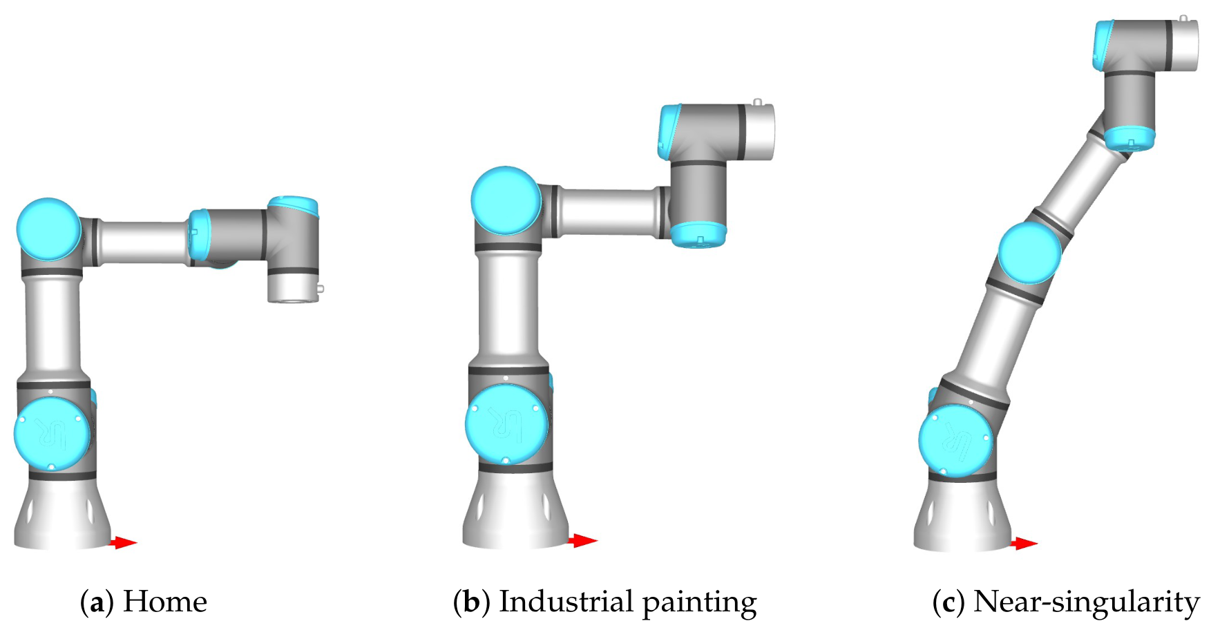
Near-singularity	${\left[\begin{array}{c}0.2954\\ -0.1104\\ 0.6380\end{array}\right]}^T$	$\left[\begin{array}{ccc}0& 0& 1\\ -1& 0& 0\\ 0& -1& 0\end{array}\right],{\left[\begin{array}{c}-69.28\\ 69.28\\ -69.28\end{array}\right]}^T$

, three representative End-Effector poses are shown, selected to capture scenarios of practical relevance for common robotic tasks. The first corresponds to the nominal home position of the UR3, which is widely used as a reset or calibration configuration. The second represents a typical orientation employed in industrial painting processes, with the tool aligned normal to the work surface to replicate real operational requirements. The third pose was deliberately chosen near a singularity, where the smallest singular value of the Jacobian becomes small, creating numerical ill-conditioning and reduced dexterity. This triad of test cases allowed evaluation of solver behavior under nominal, task-oriented, and near-singular conditions.

It is important to remark that the graphical representations in Table 4 correspond to just one of the possible articular configurations (q) that the robot may adopt to satisfy the desired EE pose (Cartesian position ${\mathbf{p}}_d$ in [m] and Orientation ${\mathbf{R}}_d$ represented as an orientation matrix and axis-angle vector in [^∘]). The joint positions shown are only representative; therefore, the solution provided by each algorithm of this methodology may result in a completely different articular configuration.

The optimization objective was the singularity-aware pose error defined in Section 3, combining translational and rotational deviations into a unified Euclidean metric with a physically meaningful angular-to-linear scaling. A smooth Jacobian-based penalty was included to discourage solutions near singular configurations. This formulation ensured that the optimization problem remained consistent and interpretable across all tested scenarios. It should be noted that while evaluating the near-singularity target, explicitly quantifying the exact degree of ill-conditioning (such as the Jacobian condition number) of the final solution is unnecessary within this metaheuristic framework. Because the cost function applies a severe discrete penalty ($+1000$) whenever the minimum singular value drops below $1\times {10}^{-4}$, the ill-conditioned regions act as hard barriers in the fitness landscape. Over 1000 independent Monte Carlo runs, the elitist selection mechanisms of the stochastic algorithms systematically discard these penalized candidate solutions. Consequently, the final optimized joint configuration ${\mathbf{q}}^{*}$ reported by the solvers is mathematically guaranteed to belong to a well-conditioned inverse kinematics branch, inherently avoiding the degenerate region.

Each run was terminated when either the maximum number of iterations was reached or the solution failed to improve within the predefined stagnation window. The outcomes of all runs were aggregated to compute descriptive statistics including the best objective, mean objective, standard deviation of the objective, mean runtime in seconds, and standard deviation of runtime. The objective-based indicators quantify solution quality and robustness, whereas runtime describes the observed computational cost of each implementation under the adopted stopping rule. Because the stagnation criterion can be activated at different iterations depending on the solver, runtime is not used as a stand-alone basis for declaring algorithmic superiority.

In addition to numerical simulations, the solutions obtained by the LM approach and the metaheuristic solvers were verified in a virtual RoboDK environment. For simulation tests, the resulting joint configurations were imported into RoboDK, where the end-effector poses were reconstructed and compared against the desired targets, allowing evaluation of kinematic accuracy and feasibility in an offline virtual prototype. For physical validation, representative GWO-based configurations were executed on a real UR3 collaborative robot under controlled laboratory conditions using the RoboDK API for MATLAB over a TCP/IPv4 network interface. The actual end-effector positions and orientations were measured using the internal encoders of the robot and verified against the desired task-space poses. This validation confirmed that the solutions were mathematically consistent and physically executable on the UR3 robot.

The statistical analysis was defined after examining the empirical behavior of the Monte Carlo results. Since the output distributions of optimization algorithms may vary depending on the solver, the target pose, and the structure of the search landscape, the use of non-parametric tests was not assumed solely from the stochastic nature of the metaheuristic methods. Instead, the distributional properties of the experimental data were first evaluated through formal diagnostic tests.

For each task pose and algorithm, the objective-function values obtained from the 1000 independent runs were tested for normality using the Shapiro–Wilk and Anderson–Darling tests. In addition, Levene’s test, using the median as the center measure, was applied to assess the homogeneity of variance across algorithms for each task pose. Since the sample size was large, these formal tests were complemented with visual diagnostics based on histograms and Q–Q plots. This combined assessment provided a more transparent interpretation of the empirical distributions, as large-sample normality tests may detect statistically significant deviations even when their practical relevance is limited.

Table 5. Normality diagnostic tests for the objective-function values obtained from 1000 Monte Carlo runs per solver and task pose.

Task Pose	Algorithm	Shapiro–Wilk p	Anderson–Darling p	Normality Assumption
Home	GWO	$2.19\times {10}^{-7}$	$3.18\times {10}^{-5}$	Rejected
Home	GA	$1.42\times {10}^{-5}$	$3.97\times {10}^{-5}$	Rejected
Home	JADE	$1.76\times {10}^{-2}$	$4.48\times {10}^{-2}$	Rejected
Home	ALO	$2.61\times {10}^{-10}$	$4.42\times {10}^{-14}$	Rejected
Home	PSO	$2.03\times {10}^{-9}$	$4.35\times {10}^{-7}$	Rejected
Industrial painting	GWO	$2.55\times {10}^{-11}$	$9.89\times {10}^{-15}$	Rejected
Industrial painting	GA	$7.00\times {10}^{-2}$	$5.90\times {10}^{-2}$	Not rejected
Industrial painting	JADE	$1.13\times {10}^{-1}$	$3.06\times {10}^{-1}$	Not rejected
Industrial painting	ALO	$2.58\times {10}^{-16}$	$6.39\times {10}^{-24}$	Rejected
Industrial painting	PSO	$3.44\times {10}^{-3}$	$3.78\times {10}^{-4}$	Rejected
Near-singularity	GWO	$3.46\times {10}^{-10}$	$1.19\times {10}^{-12}$	Rejected
Near-singularity	GA	$2.33\times {10}^{-5}$	$1.54\times {10}^{-5}$	Rejected
Near-singularity	JADE	$1.72\times {10}^{-1}$	$7.35\times {10}^{-1}$	Not rejected
Near-singularity	ALO	$2.46\times {10}^{-18}$	<$1\times {10}^{-300}$	Rejected
Near-singularity	PSO	$7.32\times {10}^{-3}$	$3.61\times {10}^{-3}$	Rejected

summarizes the normality diagnostics for the objective-function values. The results show that normality was rejected in 12 out of the 15 algorithm–pose combinations. For the home configuration, all algorithms rejected the normality assumption. For the industrial painting pose, GA and JADE did not reject normality, whereas GWO, ALO, and PSO did. For the near-singularity pose, only JADE did not reject normality. These results confirm that the distributional behavior was not uniform across algorithms or task poses, reinforcing the need to base the statistical comparison on the observed data rather than on an a priori assumption.

The variance-homogeneity analysis is reported in

Table 6. Levene’s test for homogeneity of variance across algorithms for each task pose.

Task Pose	Levene Statistic	p-Value	Variance Homogeneity
Home configuration	231.72	$9.34\times {10}^{-183}$	Rejected
Industrial painting	699.03	<$1\times {10}^{-300}$	Rejected
Near-singularity	899.25	<$1\times {10}^{-300}$	Rejected

. Levene’s test rejected the null hypothesis of equal variances for the three task poses. This indicates that, even in cases where some individual algorithm distributions did not reject normality, the assumption of homogeneous variance across algorithms was not satisfied. Therefore, the requirements for applying standard parametric comparisons were not consistently met.

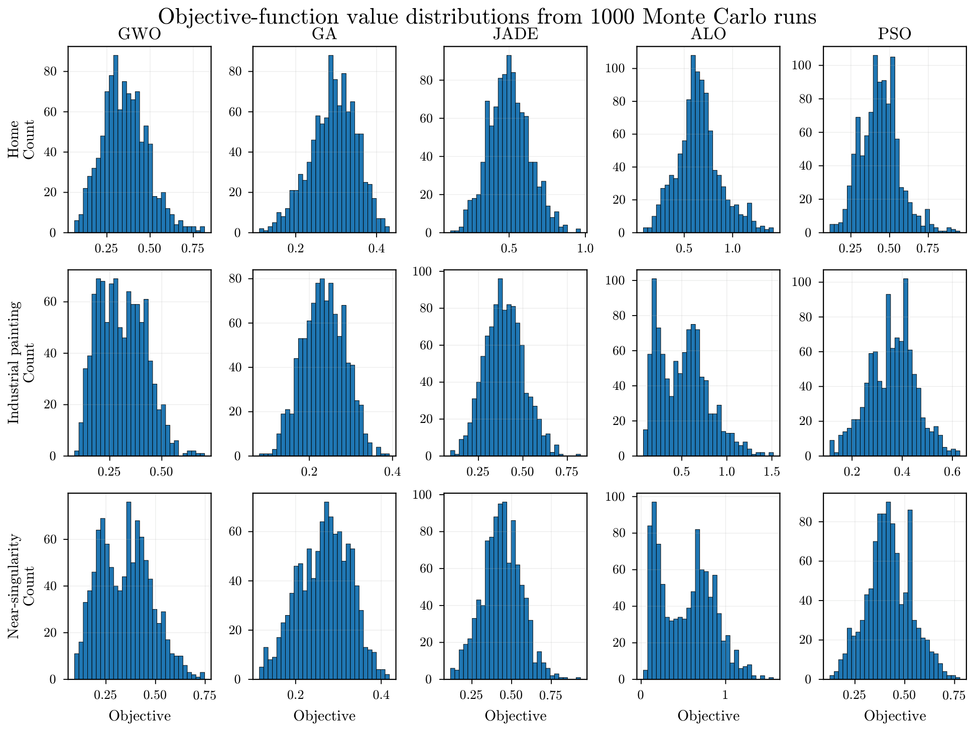
The formal diagnostic tests were also inspected together with the graphical behavior of the empirical distributions. Figure 3 shows the histograms of the objective-function values for all algorithms and task poses. The plots reveal asymmetric shapes, different dispersion levels, bounded support near zero, and occasional extreme values, particularly for some algorithm–pose combinations. These visual patterns are consistent with the results of the normality and variance-homogeneity tests.

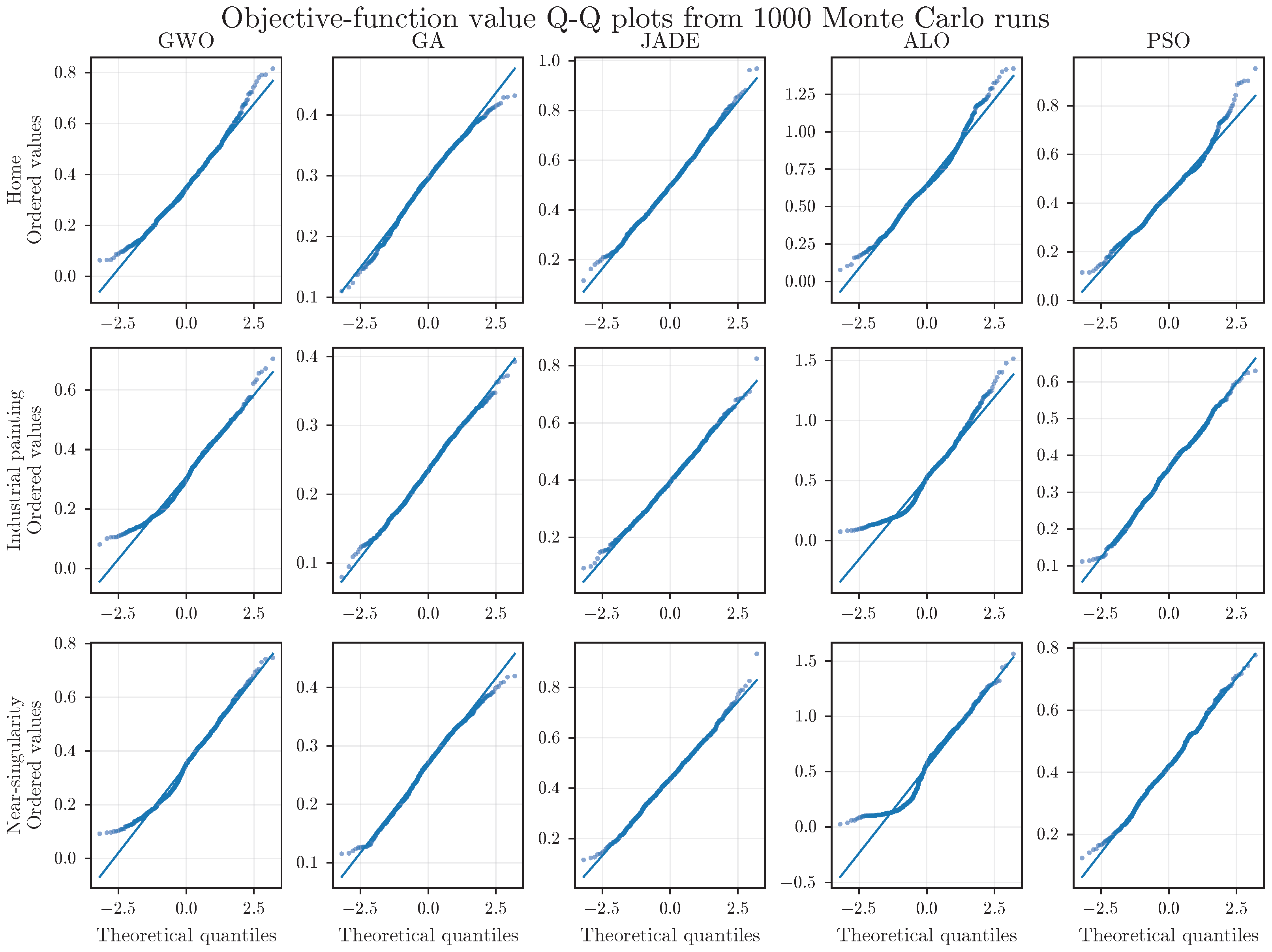
Figure 4 presents the corresponding Q–Q plots. These visual diagnostics complement the formal tests by showing deviations from the theoretical normal distribution in several cases, especially in the tails. The combined evidence from the formal and visual diagnostics supports the use of a statistical framework that does not require normality or equal variances.

Based on this diagnostic analysis, the comparative evaluation of the metaheuristic solvers was conducted using non-parametric rank-based statistics, together with descriptive indicators of accuracy, dispersion, and runtime. This decision was based on the empirical behavior of the experimental data and not on a prior assumption regarding the stochastic nature of the optimization algorithms.

6. Levenberg–Marquardt Results

To establish a rigorous performance baseline for UR3 Inverse Kinematics problem, a numerical solver based on the Levenberg–Marquardt (LM) algorithm was developed. This implementation utilizes an adaptive damping strategy (initialized at $\mu ={10}^{-3}$) to alternate between the Gauss–Newton and Gradient Descent methods, ensuring robust convergence even in the vicinity of kinematic singularities. A discrete penalty mechanism based on the Jacobian determinant was incorporated to strictly reject singular configurations during the iterative search. The experimental protocol involved testing each solver across three representative task-space poses. While the stochastic metaheuristic solvers were independently executed 1000 times to analyze their statistical consistency, the LM algorithm served as the reference standard for precision and computational speed (CPU time). The valid joint configurations obtained were verified within the RoboDK simulation environment.

6.1. Home Configuration Results

The performance of the proposed Levenberg–Marquardt algorithm was evaluated on the test trajectory. The numerical solver demonstrated superior convergence properties compared to stochastic methods. Starting from a non-singular seed configuration, the algorithm successfully converged to the target pose ${\mathbf{p}}_d$ m and rotation vector ${\mathbf{r}}_d$. The solver required only 8 iterations to minimize the error norm to $2.73\times {10}^{-13}$, effectively achieving zero geometric error within machine precision limits. The total computation time was 0.0563 s, making it highly suitable for real-time control applications where cycle times are critical. The resulting joint configuration, listed in

Table 7. Joint configuration q (^∘) obtained by LM.

Task Pose	${\mathit{q}}_1$	${\mathit{q}}_2$	${\mathit{q}}_3$	${\mathit{q}}_4$	${\mathit{q}}_5$	${\mathit{q}}_6$
Home	0.3788	−89.0745	−91.0512	−89.8745	89.9998	0.3788
Industrial painting	0.5246	−89.8211	−90.7025	0.5236	89.4754	0.0000
Near-singularity	0.5245	−111.4839	−13.8220	−54.6941	89.4755	0.0000

and depicted in Figure 5a, confirms that the solution lies well within the mechanical joint limits of the UR3 robot.

6.2. Industrial Painting Configuration

The efficiency of the Levenberg–Marquardt solver was rigorously tested on the target trajectory to establish a performance benchmark. Unlike the stochastic search patterns observed in the metaheuristic algorithms, the deterministic gradient-based approach yielded a direct convergence to the desired Cartesian state ${\mathbf{p}}_d$ and orientation ${\mathbf{r}}_d$. The solver achieved an exact kinematic solution with a residual error of $9.02\times {10}^{-13}$, effectively reaching machine precision. This level of accuracy was attained in just 6 iterations, requiring a computational time of 0.0123 s. The corresponding articular values are detailed in Table 7, the joint configuration for this pose is shown in Figure 5b.

6.3. Near-Singularity Configuration

To evaluate the performance of the optimization algorithms, this subsection focuses on the near-singularity configuration, a scenario deliberately designed to test numerical stability under severe Jacobian ill-conditioning. As a baseline, the deterministic gradient-based scheme converged directly to the desired pose. The algorithm achieved a negligible residual error of $1.90\times {10}^{-11}$ in merely 7 iterations, requiring a computational time of 0.0128 s. This performance confirms the suitability of the LM approach for high-precision tasks, provided the initial estimate avoids the singularity boundary. 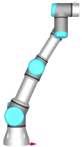The corresponding joint configuration is detailed in Table 7 and illustrated in Figure 5c.

7. Metaheuristics Results

As established in the diagnostic analysis reported in Table 5 and Table 6, the assumptions of normality and homogeneity of variance were not consistently satisfied across the evaluated algorithms and task poses. Therefore, the following comparisons are interpreted using non-parametric rank-based statistics, complemented by descriptive indicators of objective-function value, dispersion, and computational time.

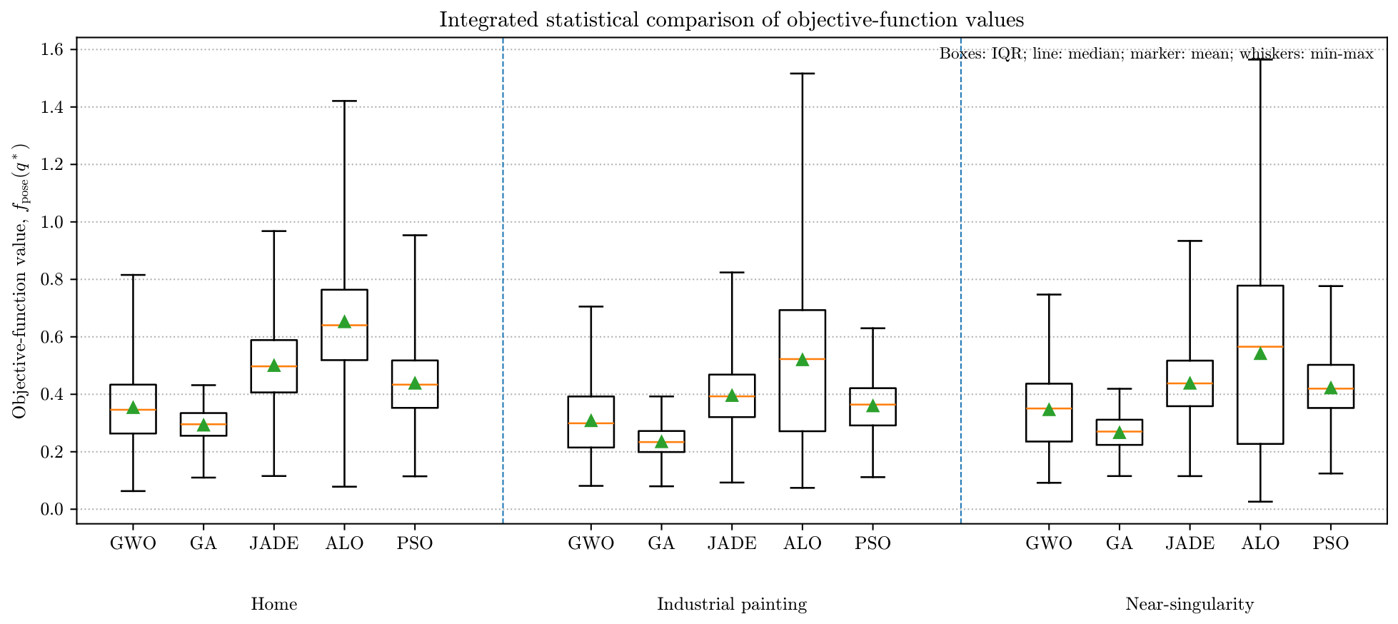
This section presents the experimental evaluation of five metaheuristic solvers, GWO, GA, JADE, ALO, and PSO, applied to the inverse kinematics problem of the UR3 manipulator. Each solver was independently executed 1000 times across three representative task-space poses. The performance was quantified using five indicators: Best Objective (minimum across runs), Mean Objective, Std Objective, Mean Time (s), and Std Time (s). Additionally, simulation validation was performed in RoboDK and subsequently replicated on a physical UR3 robot to verify practical feasibility.

Figure 6 summarizes the objective-function distributions for the five metaheuristic solvers across the three evaluated task poses. This representation combines central tendency, dispersion, and extreme-value information, allowing the reader to compare not only the average performance of each method, but also its robustness and variability across the 1000 independent runs.

7.1. Home Configuration Results

Table 8. Performance summary for the home configuration (1000 runs per solver).

Algorithm	Best Objective	Mean Objective	Std Objective	Mean Time (s)	Std Time (s)
GWO	0.063	0.354	0.130	0.79	0.86
GA	0.110	0.293	0.058	31.82	0.89
JADE	0.116	0.500	0.134	0.08	0.78
ALO	0.078	0.652	0.227	28.73	0.81
PSO	0.115	0.439	0.127	0.68	0.84

summarizes the statistical performance of the algorithms for the home configuration. This pose represents a numerically stable scenario with moderate coupling among joint variables. GA achieved the lowest mean objective and the smallest objective dispersion, while GWO obtained the best individual objective value and the second-lowest mean objective. JADE achieved the shortest mean runtime but with lower objective accuracy. ALO and PSO showed less favorable objective behavior than GA and GWO, with ALO exhibiting the largest dispersion.

The Table 8 results show that GA achieved the lowest mean objective in the home configuration, with $\overline{f}=0.293$ and the smallest objective dispersion, ${\sigma }_f=0.058$. GWO obtained the best objective value among the 1000 runs, $f_{min}=0.063$, and the second-lowest mean objective, $\overline{f}=0.354$, with moderate dispersion, ${\sigma }_f=0.130$. JADE was the fastest implementation, with a mean runtime of 0.08 s, but its mean objective increased to 0.500. PSO showed intermediate behavior, with $\overline{f}=0.439$ and a mean runtime of 0.68 s. ALO obtained a competitive best objective, $f_{min}=0.078$, but its mean objective, $\overline{f}=0.652$, and dispersion, ${\sigma }_f=0.227$, indicate less consistent convergence. Therefore, for the home pose, GA is preferable when accuracy and repeatability are prioritized, whereas JADE is preferable when runtime is the dominant constraint. GWO represents an intermediate alternative with competitive accuracy and short runtime.

The best angular positions for each DoF of the UR3 obtained by metaheuristic algorithms are shown in

Table 9. Articular configuration q (^∘) for Home Pose.

Algorithm	${\mathit{q}}_1$	${\mathit{q}}_2$	${\mathit{q}}_3$	${\mathit{q}}_4$	${\mathit{q}}_5$	${\mathit{q}}_6$
GWO	−0.4515	−180.0000	91.0766	177.4445	88.7948	−0.3674
GA	12.5839	−81.3681	−103.8308	−83.8939	93.0849	14.0764
JADE	130.6753	−19.5547	−105.9520	34.3815	−87.9702	−50.9011
ALO	−8.3015	−87.8737	−107.4880	−73.8934	89.8572	−8.4528
PSO	−1.0581	180.0000	71.5573	15.6146	-90.8973	−180.0000

.

7.2. Industrial Painting Configuration

The second pose corresponds to an industrial painting orientation, characterized by stronger coupling between position and orientation variables.

Table 10. Performance summary for the industrial painting configuration (1000 runs per solver).

Algorithm	Best Objective	Mean Objective	Std Objective	Mean Time (s)	Std Time (s)
GWO	0.081	0.308	0.111	0.77	0.85
GA	0.080	0.235	0.051	31.43	0.83
JADE	0.093	0.396	0.109	0.08	0.79
ALO	0.074	0.520	0.275	28.37	0.86
PSO	0.112	0.360	0.095	0.60	0.82

shows that GA achieved the lowest mean objective and the smallest objective dispersion, while GWO ranked second in mean objective with substantially lower runtime than GA. JADE was the fastest solver, although its objective accuracy was lower than that of GA and GWO. ALO obtained the best isolated objective value, but its high mean objective and dispersion indicate low repeatability.

For the industrial painting configuration, GA obtained the lowest mean objective, $\overline{f}=0.235$, and the smallest objective dispersion, ${\sigma }_f=0.051$, indicating the most repeatable convergence among the evaluated metaheuristics. GWO ranked second in mean objective, $\overline{f}=0.308$, and maintained a substantially shorter mean runtime, 0.77 s, compared with GA, 31.43 s. JADE remained the fastest implementation, 0.08 s, but its mean objective increased to 0.396. PSO produced an intermediate mean objective, $\overline{f}=0.360$, with a mean runtime of 0.60 s. ALO reached the best individual objective value, $f_{min}=0.074$, but its higher mean objective, $\overline{f}=0.520$, and high dispersion, ${\sigma }_f=0.275$, indicate that this best-case result was not consistently reproduced. Thus, for this orientation-demanding pose, GA provides the most accurate and stable behavior, while GWO offers a lower-time alternative with competitive objective values.

The best articular configurations for the UR3 6-DoF calculated by the algorithms are depicted in

Table 11. Articular configuration q (^∘) for Industrial Painting Pose.

Algorithm	${\mathit{q}}_1$	${\mathit{q}}_2$	${\mathit{q}}_3$	${\mathit{q}}_4$	${\mathit{q}}_5$	${\mathit{q}}_6$
GWO	−0.9086	−123.4860	−7.9025	130.8392	−91.7038	−180.0000
GA	106.6521	−61.6862	−14.3451	78.0455	18.2001	176.8703
JADE	100.6250	−18.2512	−102.0454	−56.7382	−9.3244	−1.8061
ALO	14.1237	−69.2467	−102.6699	−8.1045	75.6382	−0.0234
PSO	137.7386	−89.3839	68.2872	19.9499	47.5760	180.0000

.

7.3. Near-Singularity Configuration

The third scenario corresponds to a configuration close to a kinematic singularity, used to evaluate robustness under ill-conditioned conditions. As summarized in

Table 12. Performance summary for the near-singular configuration (1000 runs per solver).

Algorithm	Best Objective	Mean Objective	Std Objective	Mean Time (s)	Std Time (s)
GWO	0.092	0.346	0.131	0.80	1.43
GA	0.115	0.267	0.060	29.63	1.62
JADE	0.115	0.438	0.122	0.10	1.36
ALO	0.026	0.542	0.318	28.64	1.47
PSO	0.124	0.422	0.112	0.60	1.35

, GWO and GA maintain relatively stable convergence patterns, whereas PSO and ALO exhibit sensitivity to Jacobian conditioning, leading to larger error dispersion. JADE converges quickly but with reduced orientation precision.

Near the singularity region, the search landscape becomes more difficult because small changes in joint space can produce poorly conditioned Cartesian behavior. GA again achieved the lowest mean objective, $\overline{f}=0.267$, and the lowest objective dispersion, ${\sigma }_f=0.060$, confirming its accuracy and repeatability under the adopted penalty formulation. GWO obtained the second-lowest mean objective, $\overline{f}=0.346$, with moderate dispersion, ${\sigma }_f=0.131$, and a mean runtime of 0.80 s. JADE remained the fastest solver, with a mean runtime of 0.10 s, but its mean objective increased to 0.438. PSO showed similar objective behavior to JADE, with $\overline{f}=0.422$ and ${\sigma }_f=0.112$, while ALO achieved the lowest best objective, $f_{min}=0.026$, but had the highest dispersion, ${\sigma }_f=0.318$. These results indicate that the best isolated result is not sufficient to characterize solver reliability near singular configurations. Under this condition, GA provides the most consistent objective performance, whereas GWO reduces computational time substantially while retaining competitive accuracy. Finally,

Table 13. Articular configuration q (^∘) for Near-singularity Pose.

Algorithm	${\mathit{q}}_1$	${\mathit{q}}_2$	${\mathit{q}}_3$	${\mathit{q}}_4$	${\mathit{q}}_5$	${\mathit{q}}_6$
GWO	102.5226	−39.5471	−63.2496	−70.1929	−11.7954	−6.8056
GA	−16.4167	−135.8283	35.4605	−82.3065	104.5791	−2.2658
JADE	114.2960	−28.6624	−79.7585	−75.9005	−24.4211	2.4459
ALO	2.3117	−102.8410	−35.9216	−40.7895	87.5224	0.0451
PSO	99.9671	−43.7360	−58.4910	−80.7461	−9.5926	−0.7148

shows the algorithms’ best calculations for each UR3 6-DoF.

7.4. Pose Error Analysis

To provide a rigorous quantitative assessment of the solver’s precision, the Mean Squared Error (MSE) was adopted as the primary global performance metric. This indicator evaluates the element-wise deviation between the target homogeneous transformation matrix, ${\mathbf{T}}_d\in SE\left(3\right)$, and the actual EE pose, $\mathbf{T}\left(\mathbf{q}\right)$, derived from the optimized joint configuration. The error matrix is defined as $\mathbf{E}={\mathbf{T}}_d-\mathbf{T}\left(\mathbf{q}\right)$, and the MSE is computed by averaging the squared magnitude of each entry within this $4\times 4$ difference matrix:

$$MSE={\displaystyle \frac{1}{N}}{\displaystyle \sum _{i=1}^4}{\displaystyle \sum _{j=1}^4}{\left({\mathbf{T}}_d(i,j)-\mathbf{T}(i,j)\right)}^2,$$

(27)

where $N=16$ represents the total number of matrix elements. This formulation condenses both translational residuals and rotational discrepancies into a single, minimization-oriented scalar value. Consequently, an MSE value approaching zero signifies high-fidelity convergence to the desired task-space state, providing a standardized baseline to compare the stochastic performance of the metaheuristic solvers against the deterministic numerical benchmark.

Table 14. Mean Squared Error (MSE) for the tested poses.

Algorithm	Home	Industrial Painting	Near-Singularity
GWO	$2.494\times {10}^{-4}$	$4.134\times {10}^{-4}$	$5.288\times {10}^{-4}$
ALO	$3.835\times {10}^{-4}$	$3.449\times {10}^{-4}$	$4.307\times {10}^{-5}$
GA	$7.580\times {10}^{-4}$	$3.990\times {10}^{-4}$	$8.330\times {10}^{-4}$
PSO	$8.216\times {10}^{-4}$	$7.799\times {10}^{-4}$	$9.666\times {10}^{-4}$
JADE	$8.356\times {10}^{-4}$	$5.394\times {10}^{-4}$	$8.306\times {10}^{-4}$

summarizes the MSE performance for the five metaheuristic algorithms for the positions evaluated.

7.5. Nonparametric Statistical Assessment Across Poses

To provide formal statistical evidence, rank-based hypothesis testing was conducted using the 1000 independent runs available per solver and per pose. Rank-based nonparametric tests were selected because the compared samples correspond to stochastic optimization outcomes, whose empirical distributions are typically skewed, bounded below by zero, and may contain outliers associated with premature stagnation or sporadic convergence to different inverse-kinematics branches. In this context, the objective is to compare full empirical performance distributions among solvers rather than only the means. Although the large number of runs supports stable estimates of central tendency, it does not by itself guarantee normality of the underlying solver-output distributions or homogeneity of variance across algorithms. Since the same run index was available across solvers for each pose, the data were treated as paired and the Friedman test was applied to detect global differences among the five metaheuristic solvers. When the Friedman test rejected the null hypothesis, post hoc pairwise Wilcoxon signed-rank tests with Holm correction were performed. For both the objective value and runtime, lower values indicate better performance, and thus lower mean ranks correspond to better solvers.

Table 15. Summary of Friedman tests and mean-rank orderings for objective and runtime, computed from 1000 paired runs per solver and per pose. Lower mean rank indicates better performance.

Pose	Metric	${\mathit{\chi }}^2$	df	p	Best Rank	Mean-Rank Ordering, Lower is Better
Point 1	Objective	1807.4408	4	$\approx 0$	GA	GA (1.640), GWO (2.294), PSO (3.098), JADE (3.649), ALO (4.319)
Point 1	Time	3812.9032	4	$\approx 0$	JADE	JADE (1.000), PSO (2.373), GWO (2.627), ALO (4.000), GA (5.000)
Point 2	Objective	1177.5544	4	$1.1695\times {10}^{-253}$	GA	GA (1.709), GWO (2.596), PSO (3.282), JADE (3.572), ALO (3.841)
Point 2	Time	3827.3800	4	$\approx 0$	JADE	JADE (1.000), PSO (2.315), GWO (2.685), ALO (4.000), GA (5.000)
Point 3	Objective	899.6520	4	$1.9818\times {10}^{-193}$	GA	GA (1.819), GWO (2.688), PSO (3.406), JADE (3.517), ALO (3.570)
Point 3	Time	3831.3176	4	$\approx 0$	JADE	JADE (1.001), PSO (2.293), GWO (2.706), ALO (4.002), GA (4.998)

summarizes the Friedman statistics and the corresponding mean-rank orderings. In all three poses, the Friedman tests revealed statistically significant differences among solvers for both the objective and runtime. Consistently, GA achieved the best mean rank for the objective, while JADE achieved the best mean rank for runtime. These tendencies are consistent with the descriptive statistics reported in Table 8, Table 9, Table 10, Table 11 and Table 12 and remain stable across nominal, task oriented, and near singular configurations.

In the home pose, the Friedman test detected differences among solvers for the objective, ${\chi }^2\left(4\right)=1807.44$, $p\approx 0$, and for runtime, ${\chi }^2\left(4\right)=3812.90$, $p\approx 0$. GA achieved the best objective rank, GA (1.640), while JADE achieved the best runtime rank, JADE (1.000). The Holm corrected Wilcoxon post hoc tests confirmed that every pairwise comparison was significant for both objective and runtime, with $10/10$ significant pairs after correction.

For the industrial painting pose, solver differences were again significant for the objective, ${\chi }^2\left(4\right)=1177.55$, $p=1.1695\times {10}^{-253}$, and for runtime, ${\chi }^2\left(4\right)=3827.38$, $p\approx 0$. The mean ranks reproduced the same pattern observed in Point 1, with GA obtaining the best objective rank, GA (1.709), and JADE obtaining the best runtime rank, JADE (1.000). The Holm corrected Wilcoxon tests indicated $10/10$ significant pairs for both objective and runtime.

In the near singular pose, the Friedman test remained significant for the objective, ${\chi }^2\left(4\right)=899.65$, $p=1.9818\times {10}^{-193}$, and for runtime, ${\chi }^2\left(4\right)=3831.32$, $p\approx 0$. GA preserved the best objective rank, GA (1.819), and JADE preserved the best runtime rank, JADE (1.001). All Holm corrected Wilcoxon comparisons were significant, with $10/10$ pairs for objective and $10/10$ pairs for runtime. The smallest, but still significant, objective difference was observed for JADE vs PSO, with $p_{\mathrm{Holm}}=2.07\times {10}^{-3}$, indicating that these two solvers become closer in objective performance under near singular kinematics while remaining statistically distinguishable under the adopted paired design.

These results support two technical conclusions. First, the ranking of solvers by objective quality is stable across poses, with GA achieving the best mean rank in all three configurations and GWO consistently occupying the second position. Second, the ranking by runtime is also stable, with JADE being the fastest, followed by PSO and GWO. Since the tests were applied to 1000 paired runs per solver and per pose, the performance distributions are well resolved, and the resulting conclusions are not driven by isolated best cases but by reproducible differences across repeated trials.

7.6. Integrated Interpretation of Solver Performance

The results are interpreted directly from the descriptive statistics in Table 8, Table 9, Table 10, Table 11 and Table 12 and from the mean-rank orderings in Table 15. This avoids assigning subjective weights to accuracy, stability, and runtime. The resulting interpretation is therefore metric-specific rather than dependent on a single aggregate index.

Across the three tested poses, GA consistently achieved the lowest mean objective values and the smallest objective dispersions. The mean objective values were 0.293, 0.235, and 0.267 for the home, industrial painting, and near-singular configurations, respectively. This indicates that GA was the most accurate and repeatable metaheuristic solver under the adopted objective function. However, GA also had the largest mean runtime, ranging from 29.63 s to 31.82 s, which limits its suitability for rapid computation.

JADE exhibited the lowest mean runtime across all configurations, ranging from 0.08 s to 0.10 s. Nevertheless, this computational advantage was accompanied by higher mean objective values than GA and GWO. Therefore, JADE is appropriate when execution time is the primary requirement and a moderate loss in pose accuracy is acceptable.

GWO provided an intermediate behavior across all test cases. Its mean objective values were consistently second-best after GA, while its runtime remained below 1s in all three configurations. This makes GWO a suitable compromise when both accuracy and computational time must be considered, but this conclusion is stated as a table-based interpretation rather than as the result of a weighted aggregate score.

PSO showed intermediate runtime and objective values, but it did not outperform GWO in objective quality or JADE in runtime. ALO produced competitive isolated best values in some cases, especially in the near-singular configuration, but its higher mean objective and larger dispersion indicate lower repeatability. Consequently, solver selection should be task-dependent: GA is preferable for accuracy and repeatability, JADE for minimum runtime, and GWO for a compromise between both criteria.

7.7. Computational Cost Analysis

The computational complexity of the evaluated metaheuristic algorithms can be analyzed using Big-O notation by considering the dominant operations performed during each iteration. For all solvers, the main computational burden arises from evaluating the objective function, which requires computing the forward kinematics, the Jacobian matrix, and the pose-error residual for each candidate solution.

Let N denote the population size, $T_{max}$ the maximum number of iterations, d the number of decision variables, which in this study is fixed to $d=6$, and $C_f$ the computational cost associated with a single evaluation of the objective function. Since each algorithm evaluates the objective function once per individual at every iteration, the dominant computational cost for all considered solvers can be expressed as

$$\mathcal{O}\left(N{T}_{max}{C}_f\right).$$

(28)

The cost $C_f$ itself is primarily determined by the forward kinematics and Jacobian computation, both of which scale approximately linearly with the number of joints, yielding $C_f=\mathcal{O}\left(d\right)$. Therefore, the overall asymptotic computational complexity of the evaluated metaheuristic solvers becomes

$$\mathcal{O}\left(N{T}_{max}d\right).$$

(29)

The runtime values reported in Table 8, Table 9, Table 10, Table 11 and Table 12 should be interpreted with caution. Although all solvers share the same asymptotic upper-bound complexity, $\mathcal{O}\left(N{T}_{max}d\right)$, the practical number of executed iterations can differ because the same early-stopping rule is applied to all algorithms. Therefore, the runtime values reflect the combined effect of the algorithmic update equations, implementation overhead, and solver-dependent activation of the stagnation criterion. In this study, all solvers were evaluated using the same values of N, $T_{max}$, joint limits, objective function, and stopping rule; however, this does not imply that every solver consumed the same number of objective-function evaluations in every Monte Carlo run. For this reason, runtime is reported as a descriptive computational metric and is not used as a weighted component in the final solver ranking.

7.8. Simulation and Physical Validation

All optimized configurations were tested in RoboDK to verify the reachability and kinematic feasibility of the resulting joint vectors. The virtual simulations confirmed that the computed inverse kinematics accurately matched the target poses with millimeter positional error. Subsequently, the same articular configurations were deployed on a real UR3 robot, confirming that no joint-limit violations or unstable motions occurred during execution. GWO was selected for experimental validation because it provided a compromise between objective quality and computational time, with lower mean objective values than JADE and PSO and substantially shorter runtime than GA and ALO. 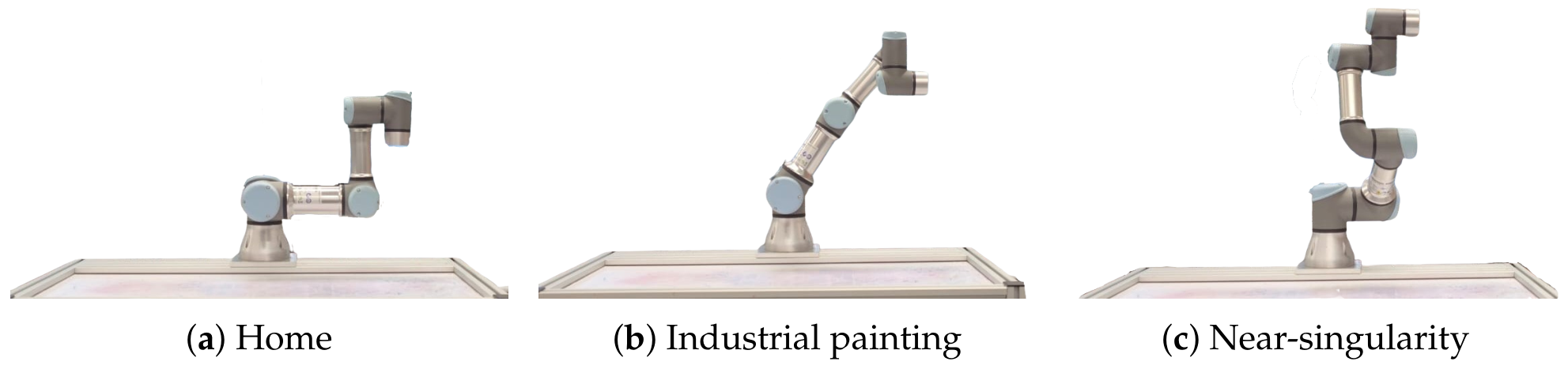Figure 7 shows the physical results obtained by this algorithm for the three tested poses.

Furthermore, for the physical validation phase, a robust bidirectional communication architecture was established between the workstation and the actual UR3 collaborative robot. Both the PC running the MATLAB-RoboDK interface and the UR3 controller were connected to the same local area network via TCP/IPv4. This network configuration allowed the system to send real-time, optimized joint commands to the physical cobot while simultaneously enabling bidirectional telemetry feedback, ensuring that the computed trajectories were not only mathematically sound but also kinematically executable on the physical hardware. In other words, the physical experiments confirmed that the optimization-based inverse kinematics method provides feasible and reproducible trajectories for both regular and near-singular configurations.

To quantitatively substantiate the physical validation, the final achieved end-effector poses were extracted directly from the physical UR3 controller using the real-time joint encoder data.

Table 16. Physical execution error for the three static poses using the GWO solver.

Task Pose	Translational Error (mm)	Rotational Error (∘)
Home	41.17	1.91
Industrial painting	76.75	0.97
Near-singularity	84.92	1.64

reports the absolute discrepancy between the desired theoretical targets and the physically executed poses for the three representative static GWO solutions. The translational error corresponds to the Euclidean norm of the Cartesian position error $\parallel {\mathbf{e}}_p{\left(q\right)\parallel }_2$ (expressed in millimeters), while the rotational error corresponds to the angular magnitude of the orientation deviation ($\theta$), consistent with the axis-angle representation defined in Section 3.4.

As shown in the data, the metaheuristic solver exhibits translational discrepancies in the order of 4 to 8.5 cm (41.17 to 84.92 mm) and rotational errors consistently below 2 degrees. While deterministic gradient-based methods like LM achieve sub-millimeter precision under ideal conditions, these deviations are a known characteristic of zero-order population-based solvers. As established earlier in this study, this level of precision is physically acceptable for operational tasks that tolerate moderate translational bounds. More importantly, this empirical data highlights the fundamental trade-off of employing metaheuristics in inverse kinematics: sacrificing exact mathematical millimeter precision in exchange for obtaining safe, physically feasible joint configurations that robustly avoid Jacobian singularities and provide derivative-free global convergence.

Furthermore,

Table 17. Comparison between the obtained poses in RoboDK (${\mathbf{p}}_1$) and the physical poses obtained in the UR3 robot (${\mathbf{p}}_2$) using the GWO solver.

Task Pose	Obtained Pose (RoboDK)		Obtained Pose (Physical UR3)
	${\mathbf{p}}_1$(m)	Axis-Angle (°)	${\mathbf{p}}_2$(m)	Axis-Angle (°)
Home configuration	${\left[\begin{array}{c}0.319989\\ -0.114642\\ 0.280354\end{array}\right]}^T$	${\left[\begin{array}{c}125.858\\ -126.022\\ -0.329\end{array}\right]}^T$	${\left[\begin{array}{c}0.319991\\ -0.114713\\ 0.28034\end{array}\right]}^T$	${\left[\begin{array}{c}126.54\\ -125.319\\ -0.346\end{array}\right]}^T$
Industrial Painting	${\left[\begin{array}{c}0.35506\\ -0.113595\\ 0.430726\end{array}\right]}^T$	${\left[\begin{array}{c}-70.051\\ 69.105\\ -69.426\end{array}\right]}^T$	${\left[\begin{array}{c}0.35506\\ -0.113671\\ 0.430711\end{array}\right]}^T$	${\left[\begin{array}{c}-70.044\\ 69.117\\ -68.437\end{array}\right]}^T$
Near-singularity	${\left[\begin{array}{c}0.222854\\ -0.122184\\ 0.595465\end{array}\right]}^T$	${\left[\begin{array}{c}-70.68\\ 69.755\\ -67.966\end{array}\right]}^T$	${\left[\begin{array}{c}0.222861\\ -0.122257\\ 0.595442\end{array}\right]}^T$	${\left[\begin{array}{c}-70.667\\ 69.769\\ -67.958\end{array}\right]}^T$

presents the complete Cartesian vectors for both the poses computed in the RoboDK simulation (${\mathbf{p}}_1$) and those physically measured by the UR3 robot’s internal encoders (${\mathbf{p}}_2$). As observed, the numerical discrepancy between the digital twin and the physical hardware is practically negligible (at the sub-millimeter level). This demonstrates that the physical UR3 controller accurately tracked the commanded joint variables, confirming that the centimeter-level deviations reported in Table 16 are strictly an inherent characteristic of the metaheuristic solver’s mathematical convergence, rather than an artifact of a simulation-to-reality execution gap.

7.9. Trajectory Validation with GWO

To directly address the practical engineering implications of the proposed metaheuristic framework, a sequential trajectory tracking scenario was evaluated. Rather than focusing solely on isolated point-to-point convergence, this section demonstrates the robustness and stability of the GWO algorithm, which was selected as a compromise solver because it provided competitive objective values with substantially shorter runtime than GA and ALO across the evaluated static poses. This evaluation bridges the gap between static optimization metrics and real-world operational requirements by demanding consistent kinematic feasibility across sequentially linked targets.

The designed trajectory encompasses a diverse set of Cartesian positions and complex orientation shifts distributed throughout the UR3 dexterous workspace. To further substantiate the practical viability of these solutions, the optimized joint sequences were fully executed in the offline virtual environment (RoboDK) and successfully deployed on the physical UR3 collaborative robot, without joint-limit violations or mechanical instability, connecting RoboDK and MATLAB, as previously experimented with. Supplementary Video Materials demonstrating this physical and virtual execution are provided alongside this manuscript.

For the experimental execution, the UR3 manipulator first departs from a standard, safe home configuration. From this resting state, the robot computes and executes the transition toward the designated Initial pose (Pose 1), which establishes the operational baseline for the continuous multi-pose task. The complete sequence consists of the four distinct task-space waypoints detailed in

Table 18. Sequential task-space poses for GWO trajectory validation.

Pose	Description	${\mathit{p}}_{\mathit{d}}$ (m)	${\mathit{R}}_{\mathit{d}}$
1	Initial pose	${\left[\begin{array}{c}0.2954\\ -0.1104\\ 0.3131\end{array}\right]}^T$	$\left[\begin{array}{ccc}0& -1& 0\\ -1& 0& 0\\ 0& 0& -1\end{array}\right]$
2	Intermediate 1	${\left[\begin{array}{c}0.1104\\ 0.2964\\ 0.3131\end{array}\right]}^T$	$\left[\begin{array}{ccc}0& -1& 0\\ -1& 0& 0\\ 0& 0& -1\end{array}\right]$
3	Intermediate 2	${\left[\begin{array}{c}-0.2130\\ 0.1928\\ 0.4789\end{array}\right]}^T$	$\left[\begin{array}{ccc}0.9959& -0.0904& 0\\ 0& 0& 1\\ -0.0904& -1& 0\end{array}\right]$
4	Final approach	${\left[\begin{array}{c}-0.3838\\ -0.0408\\ 0.2462\end{array}\right]}^T$	$\left[\begin{array}{ccc}-0.3857& 0.7348& -0.5578\\ 0.9226& 0.3072& -0.2332\\ 0& -0.6045& -0.7965\end{array}\right]$

, confirming physically executable joint configurations across drastically changing spatial requirements.

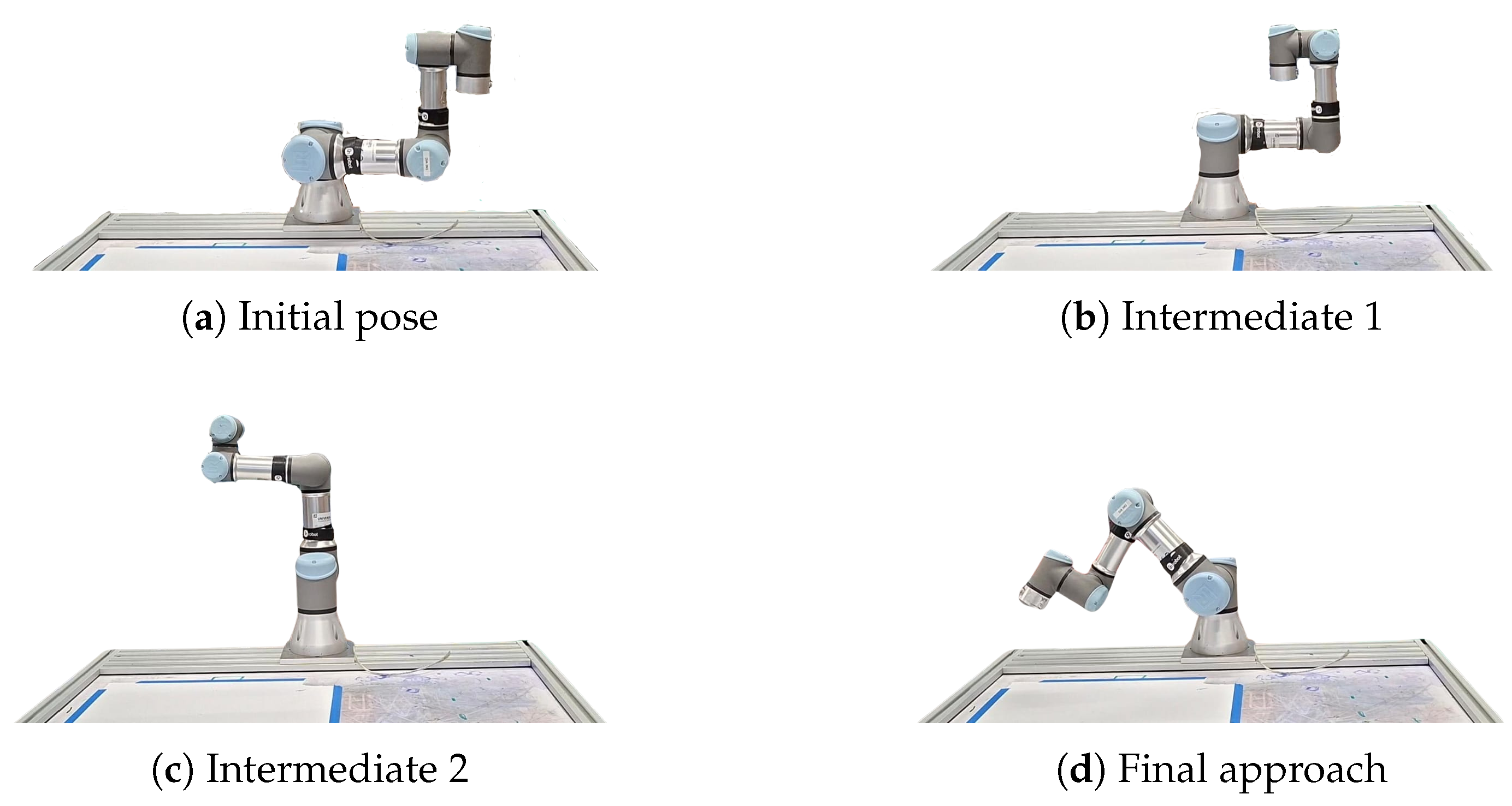
To visually substantiate the kinematic viability of the GWO-optimized solutions, the physical execution of the continuous sequence is illustrated in Figure 8. This multi-panel representation captures the robot at each critical waypoint, progressing from the initial operational baseline through the complex intermediate spatial reconfigurations, and culminating in the final approach. This visual evidence confirms that the stochastic solver not only achieves strict numerical convergence but also yields physically safe and coherent articular configurations, effectively navigating the UR3 workspace without erratic joint movements or mechanical stress between sequential targets.

To quantitatively assess the trajectory tracking performance, the Mean Squared Error (MSE) defined in Equation (27) was computed for each sequential target. The MSE condenses both positional deviations and rotational discrepancies into a unified metric, providing a strict measure of pose fidelity.

Table 19. Mean Squared Error (MSE) achieved by the GWO solver during the trajectory task.

Task Pose	MSE
Pose 1 (Initial pose)	$2.49\times {10}^{-4}$
Pose 2 (Intermediate 1)	$2.44\times {10}^{-3}$
Pose 3 (Intermediate 2)	$9.70\times {10}^{-5}$
Pose 4 (Final approach)	$1.37\times {10}^{-3}$

summarizes the error obtained by the GWO solver across the evaluated trajectory.

To guarantee full reproducibility of this continuous multi-pose task,

Table 20. Articular configurations q (^∘) for the sequential trajectory task computed by the GWO solver.

Task Pose	${\mathit{q}}_1$	${\mathit{q}}_2$	${\mathit{q}}_3$	${\mathit{q}}_4$	${\mathit{q}}_5$	${\mathit{q}}_6$
Pose 1 (Initial pose)	−10.4824	−180.0000	88.7667	180.0000	91.2135	−8.8597
Pose 2 (Intermediate 1)	−180.0000	3.6097	−93.7201	180.0000	89.9969	−180.0000
Pose 3 (Intermediate 2)	180.0000	−90.9639	−84.6565	−0.8739	−1.1459	2.5511
Pose 4 (Final approach)	−5.6293	−48.4599	106.6198	180.0000	−75.6797	−23.2181

details the exact articular configurations computed by the GWO solver for each consecutive waypoint. These angles represent the continuous spatial mapping executed by the physical UR3 controller to navigate the defined trajectory.

The numerical results demonstrate high-fidelity pose tracking throughout the continuous task. The MSE values consistently remain within the bounds of ${10}^{-3}$ to ${10}^{-5}$, indicating that the GWO algorithm successfully manages drastic orientation shifts and diverse position changes without experiencing numerical divergence. Notably, the solver achieved an exceptionally low MSE of $9.70\times {10}^{-5}$ at the second intermediate pose, confirming its precision even during complex spatial reconfigurations. This stable error profile across sequential targets validates the engineering feasibility of deploying the zero-order GWO solver for continuous robotic operations, extending its applicability beyond isolated point-to-point convergence.

The operation of the robotic prototype during the experimental validation is provided as Supplementary Video.

8. Conclusions

This work presented a singularity-aware inverse kinematics formulation for the UR3 collaborative robot together with a unified comparative study of five population-based metaheuristic solvers and a deterministic Levenberg–Marquardt (LM) baseline. The evaluation was conducted under common maximum computational settings, with population size $N=30$, maximum iteration budget $T_{max}=500$, and 1000 independent Monte Carlo runs per solver and per pose. This protocol provided statistically stable performance characterization across nominal, industrial, and near-singular configurations, allowing the shared early-stopping criterion to influence the practical number of iterations executed.

The deterministic LM solver demonstrated superior numerical precision and computational speed. For the evaluated poses, it converged within 6–8 iterations, achieving residual errors of $2.73\times {10}^{-13}$ (home), $9.02\times {10}^{-13}$ (industrial painting), and $1.90\times {10}^{-11}$ (near-singular), with execution times of 0.0563 s, 0.0123 s, and 0.0128 s, respectively. These results confirm its suitability for high-precision, real-time applications where millisecond-level response is required.

In contrast, the metaheuristic solvers provided derivative-free global search capabilities under a black-box formulation. Across all poses and based on 1000 paired runs per solver, the Friedman tests revealed statistically significant differences for both objective and runtime metrics. GA consistently achieved the best mean-rank position for objective value in all configurations, while JADE obtained the best mean-rank position for runtime. Consequently, the final interpretation is metric-specific: GA is the strongest solver in terms of objective accuracy and repeatability, JADE is the fastest implementation, and GWO provides a competitive intermediate profile with lower objective values than JADE and PSO and markedly shorter runtime than GA and ALO.

Mean Squared Error (MSE) values for the metaheuristic solutions remained on the order of ${10}^{-4}$ across the tested poses, confirming acceptable pose fidelity under stochastic optimization. These results show that GA excels in raw accuracy and repeatability, JADE in execution time, and GWO in providing a competitive compromise between objective quality and runtime without relying on a subjective weighted score.

A central outcome of this study is therefore not merely the ranking of individual algorithms, but the establishment of a reproducible and statistically grounded benchmarking framework. The combination of large-scale Monte Carlo experimentation, descriptive table-based analysis, and nonparametric hypothesis testing provides a transparent methodology for evaluating solvers under a common maximum budget and a shared stopping criterion.

Results confirm that the proposed numerical scheme is approximately three orders of magnitude faster than population-based methods, making it the preferred choice for real-time applications requiring millisecond-level latency. However, this performance comes at the cost of implementational complexity and dependency on differential kinematics. The Levenberg–Marquardt method relies heavily on gradient-flow information, requiring the analytical derivation of the Jacobian matrix and a geometrically consistent definition of the orientation error vector. In contrast, the evaluated metaheuristic solvers operate as zero-order optimizers that treat the robotic mechanism as a black box and require only the Forward Kinematics model. This characteristic allows for a simpler problem definition, where the orientation error can be intuitively computed as the element-wise difference between the current and desired rotation matrices without concern for differentiability. Therefore, while LM is indispensable for the high-speed control of standard rigid manipulators, this study successfully establishes the UR3 as a controlled validation platform for stochastic solvers. Proving their baseline accuracy and stability here is a necessary step before deploying these zero-order algorithms to highly constrained or non-differentiable scenarios, such as soft robotics, hyper-redundant arms, or dynamic collision avoidance, where analytical Jacobian methods inherently fail.

Dual validation in a RoboDK virtual environment and on a physical UR3 collaborative robot confirmed that the optimized joint configurations are not only numerically consistent but also physically implementable in realistic cobotic operation scenarios. These findings support the proposed framework as a reproducible benchmark for metaheuristic-based inverse kinematics optimization in collaborative robotics.

The findings of this study must be contextualized within the broader landscape of robotic control. The experimental results clearly show that for the standard, unconstrained UR3 inverse kinematics problem, the Levenberg–Marquardt method remains the most computationally efficient solution. The practical engineering value of the evaluated metaheuristics does not lie in substituting classical methods for standard 6-DoF tasks, but in providing a robust alternative for ill-conditioned and mathematically discontinuous environments. The successful physical execution and sequential trajectory validation of the GWO solver prove that metaheuristics can maintain high-fidelity pose tracking without generating erratic joint behaviors.

Despite these contributions, the present study exhibits limitations that should be acknowledged. First, the benchmarking analysis was conducted on a representative but finite set of task-space configurations rather than on an exhaustive sampling of the entire robot workspace. Second, the objective function was designed to ensure accurate pose satisfaction without explicitly enforcing additional operational criteria such as manipulability maximization, joint-torque minimization, or trajectory smoothness. Third, the comparative framework focused on solver-level performance indicators and did not include operator-level evolutionary diagnostics, which could provide deeper insight into the internal search dynamics of the algorithms. Future research will extend the proposed benchmarking framework in several directions. In addition to incorporating multi-objective formulations that consider manipulability, joint effort, and energy consumption, forthcoming studies will integrate operator-level evolutionary diagnostics, including EvoMapX-type metrics such as Operator Attribution Matrices, Convergence Driver Scores, and Population Evolution Graphs, particularly in analyses involving homogeneous algorithm families or hybrid adaptive variants where operator attribution can be consistently defined across solvers. Additional work will also explore large-scale workspace sampling, real-time implementations using reduced-order solvers, and hybrid approaches that combine analytical inverse-kinematics initialization with metaheuristic refinement. These extensions will further enhance the interpretability, scalability, and applicability of the proposed benchmarking methodology for collaborative robotic systems.