Machine Learning-Based Static Performance Prediction of Bonded Structural Patch Repairs

Abstract

This study investigates adhesively bonded composite patch repair to enhance the load-carrying capacity of damaged metallic structures, introducing a novel FE-augmented machine learning (ML) framework that addresses the limited availability of experimental data in structural repair applications. To evaluate this approach, aluminum and steel specimens with central fatigue cracks were repaired using glass-fiber/epoxy and carbon-fiber/epoxy composite patches and tested under quasi-static loading at room ($70 \mathrm{F} °$), high ($145 \mathrm{F} °$), and low (−$60 \mathrm{F} °$) temperatures. Finite element (FE) models were then developed in ABAQUS© to predict the failure loads of the patched specimens under varying temperature conditions, showing excellent agreement with the experimental data. The high accuracy of the FE predictions enabled their use as additional training data, effectively augmenting the limited experimental dataset and allowing the development of more robust regression models. Ten machine learning (ML) regression models, including linear regression (LR), polynomial regression (PR), support vector regression (SVR), random forest (RF), gradient boosting (GB), XGBoost (XGB), LightGBM (LGBM), Gaussian process (GP) regression, artificial neural networks (ANNs), and Kolmogorov–Arnold networks (KANs), were trained to predict the failure load of both unpatched and patched specimens as a function of material type, temperature, specimen thickness, crack length, and, for patched specimens, patch type and thickness. The datasets combined a limited set of physical results (75 patched samples: 63 experimental and 12 finite-element; 72 unpatched samples: 27 experimental and 45 theoretical) with Gaussian-mixture-model synthetic samples used only to augment the training data up to 300 samples per case. Under a configuration-grouped, leakage-free nested cross-validation (entire configurations held out for testing, hyperparameters tuned on inner folds only), the best models predicted the failure load of unseen configurations with mean absolute percentage errors of 2.78% (Gradient Boosting, patched, $R^2=0.87$) and 3.33% (Gaussian Process, unpatched, $R^2=0.98$). A paired ablation showed that Gaussian-mixture-model augmentation did not improve accuracy and, for several models, actually reduced it; the final models therefore rely on the real multi-source (experimental, FE, and theoretical) data, with the synthetic pipeline reported as a validated but non-beneficial component for these datasets. Overall, this study provides a novel, data-efficient framework combining experimental testing, FE simulation, and validated regression modeling to predict the performance of adhesively bonded composite patch repairs under varying thermal and mechanical conditions.

1. Introduction

Adhesively bonded composite patch repair is a practical temporary method to restore the structural performance of damaged components in aircraft and vehicles, allowing continued operation until permanent repair or replacement can be performed. This approach offers improved load transfer, higher fatigue resistance, and improved corrosion resistance compared to traditional mechanical fastening techniques. Despite these advantages, predicting the performance of bonded repairs under varying environmental and mechanical conditions remains challenging. The performance of repaired structures depends on several interacting parameters, including substrate material, adhesive properties, patch configuration, and temperature, all of which can influence load transfer across the bonded interface. Composite patches offer high strength-to-weight ratios, improved corrosion resistance, and adaptability to complex geometries, making them attractive candidates in aerospace, automotive, and civil engineering applications [1,2,3]. Unlike traditional mechanical fastening methods, bonded repairs reduce stress concentrations and help prevent further damage near fastener holes. In addition, bonded repairs redistribute stresses and slow crack growth, thus extending the fatigue life of damaged metal structures [4,5]. The effectiveness of bonded composite repairs depends on factors such as patch and substrate types and thicknesses, adhesive properties, surface preparation, and curing conditions [6].

The influence of patch and substrate thickness on structural performance has been widely examined in the literature. Researchers in [7] demonstrated that the effectiveness of bonded repairs is strongly dependent on the thickness of the panel: while thin panels exhibited a 236% increase in crack growth life using a 16-layer patch, thick panels showed only a 23–55% improvement with a 4-layer patch. Similarly, the experimental study in [8] on 2024-T3 aluminum plates repaired with carbon/epoxy patches (four, six and eight plies) reported that fatigue life improved with increasing patch thickness, reaching nearly a threefold improvement with eight plies. However, the authors emphasized that excessive patch stiffness can lead to new stress concentrations, highlighting the need for optimal patch thickness selection. Xiong and Shenoi [9] also confirmed that patch thickness significantly affects both static and fatigue strength, whereas the fiber-reinforced composite material primarily governs fatigue performance. In addition to patch thickness, substrate thickness significantly influences crack growth behavior. Broek and Schijve [10] demonstrated that cracks propagate more rapidly in thicker substrates, indicating a strong relationship between substrate thickness and crack growth rate. Furthermore, Kan and Ratwani [11] found that specimens with greater thickness (6.4 mm) exhibited shorter crack growth lives compared to those with smaller thickness (3.1 mm), emphasizing the critical importance of both patch and substrate thickness in bonded composite repairs.

Another important design aspect in bonded repair applications is the patch configuration. Experimental studies [12,13,14,15,16] have compared single and double-sided repair schemes and shown that double-sided repairs typically result in superior mechanical performance. Compared to unrepaired specimens, single-sided repairs increase ultimate load capacity by approximately 7%, whereas double-sided configurations provide around 12% higher strength and nearly double the fatigue life due to a greater reduction in stress intensity factors. However, when accessibility to both sides of the structure is limited, single-sided repairs remain a practical and effective solution. Considering these findings and accessibility limitations, this study employed a single-sided repair configuration to simulate realistic field repair conditions.

Bonded composite repair has been established as a reliable method for restoring structural integrity in aging metallic components. However, its effectiveness is significantly affected by environmental conditions. Near the adhesive’s glass transition temperature, both stiffness and bond strength decrease, whereas at low temperatures, the adhesive becomes more brittle. Our previous studies [17,18] demonstrated that bonded repairs on Al 6061 and A36 steel enhance load capacity at room and low temperatures, but their efficiency declines at elevated temperatures due to adhesive softening. Accurately predicting the performance of bonded repairs under these varying conditions remains a significant challenge.

In addition to the experimental investigations, several numerical studies have been conducted using the finite element method (FEM) to analyze the behavior of cracked metallic structures repaired with bonded composite patches. In previous studies, finite element analyses showed that patch geometry, adhesive properties, patch configuration, and material type significantly influence stress distribution, load transfer, and crack propagation behavior. Analyses focusing on patch thickness and geometry show that increasing patch thickness or width reduces the stress intensity factor (SIF) and delays crack growth, while excessive adhesive thickness or stiffness limits load transfer and decreases repair efficiency [19,20,21,22]. Adhesive thickness was also found to be a key factor influencing repair efficiency. Studies reported that thinner adhesive layers enhance stress transfer between the patch and substrate, leading to lower stress intensity factors and improved fatigue life, whereas thicker adhesive layers reduce load transfer and lower the overall repair efficiency [23]. Belhouari et al. [24] demonstrated that double-sided symmetric patches achieve higher SIF reduction and alleviate bending effects typically observed in single-sided repairs, leading to more balanced stress distributions. In [25], the influence of composite patch material and fiber orientation was investigated, and it was shown that boron epoxy patches outperform graphite epoxy alternatives, while fibers oriented perpendicular to the crack path enhance SIF reduction by more than 50%. Three-dimensional finite element models have improved prediction accuracy by capturing out-of-plane deformations and complex stress states near the crack front, overcoming the limitations of simplified two-dimensional analyses [26]. Overall, the findings demonstrate that finite element modeling (FEM) is a critical method for optimizing patch geometry, adhesive selection, and configuration to improve the structural integrity and durability of bonded composite repairs.

Although finite element modeling offers significant insight into the mechanical response of bonded repairs, recent developments in data-driven approaches, particularly artificial neural networks (ANNs) and other modern regression techniques, have enabled more efficient and accurate prediction of fatigue and damage behavior. In contrast to conventional S-N curves or fracture mechanics-based methods, these models can capture nonlinear interactions among multiple influencing factors, including material properties, crack geometry, loading conditions, and environmental effects. Recent studies [27,28] utilized ANN and other machine learning models to predict the fatigue life of functionally graded materials, demonstrating strong agreement between predicted and experimental results. In [29], an ANN-based model demonstrated reliable predictions of fatigue life for composite materials under variable amplitude loading. In addition, ANN models have achieved accurate fatigue life estimation for multidirectional glass fiber-reinforced laminates [30] and for various composite systems using alternative machine learning approaches such as polynomial classifiers [31]. In [32], a multilayer feedforward ANN successfully predicted the low-cycle fatigue life of Al-Si-Mg alloys, identifying key material and processing parameters influencing fatigue performance. A hybrid approach combining ANN with finite element models further improved repair evaluation accuracy and reduced experimental effort in composite patch repairs [33]. Moreover, ANNs have been applied to efficiently predict fracture mechanics parameters such as the J-integral from finite element results [34]. Recent work has further demonstrated that ANN models trained using finite element-derived fracture parameters can accurately predict mixed-mode fracture loads, outperforming conventional linear elastic fracture criteria while significantly reducing experimental effort [35]. These previous studies have shown that machine learning techniques can improve prediction accuracy and reduce experimental requirements when assessing the fatigue and damage behavior of bonded composite repairs. In light of these findings, this study combines experimental data with finite-element modeling results to develop a machine-learning-based method for predicting the static performance of bonded structural patch repairs in different environmental conditions.

2. Experimental Methodology

2.1. Materials

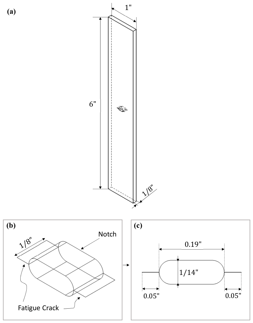
Two substrate materials were selected for this study: Al 6061 and A36 steel. Al 6061 specimens were prepared in two thicknesses, 1/8 inch (3.18 mm) and 0.190 inches (4.83 mm), while A36 steel specimens were 1/8 inch (3.18 mm) thick. Each specimen was machined with a central 0.19-inch notch, followed by fatigue loading to produce 0.05-inch cracks on each side of the notch, resulting in a total crack length of $2a=0.29$ inches. The configuration and dimensions of the unpatched specimens are presented in Figure 1.

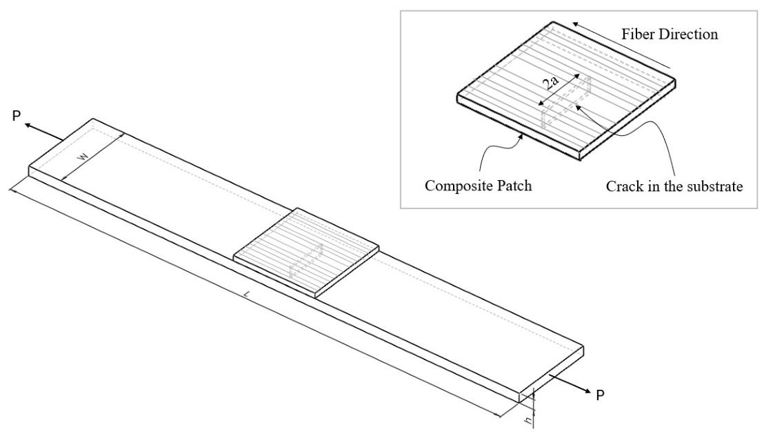
The composite patches were fabricated in-house using the vacuum infusion process. Two glass-fiber/epoxy panels with thicknesses of 1.0 mm and 1.64 mm, as well as a carbon-fiber/epoxy patch of approximately 0.89 mm, were produced from unidirectional fiber fabrics. Surface preparation to ensure strong adhesion was applied exclusively to the metallic substrates, involving acetone cleaning, sandblasting with 54–60 grit alumina oxide at 80–100 psi, and debris removal using compressed gas. The patches were bonded with Hysol EA 9309NA (Henkel Corporation, Madison Heights, MI, USA) a two-part aerospace-grade epoxy adhesive, and oven-cured at $\mathrm{66} °\mathrm{C}$ for 1 h. Testing was conducted after a 48 h post-cure period. The configuration and fiber orientation of the patched specimens are presented in Figure 2. Fibers were aligned perpendicular to the crack direction to maximize load transfer.

2.2. Experimental Setup

Static tensile tests were conducted to evaluate the load-carrying capacity of both patched and unpatched specimens. All specimens featured a central crack (a = 0.145 inches) and were loaded to failure using a universal Instron testing machine at a constant crosshead speed of 2 mm/min. The testing was performed at three temperatures: room temperature (70 °F), high temperature (145 °F), and low temperature (−60 °F), using an environmental chamber. Specimens were exposed for at least 30 min at the target temperature to achieve thermal equilibrium. The temperature was monitored using thermocouples attached to both the patched specimens and the chamber. Force and displacement data were collected, and patch performance was assessed by comparing failure loads of patched and unpatched specimens.

2.3. Experimental Results

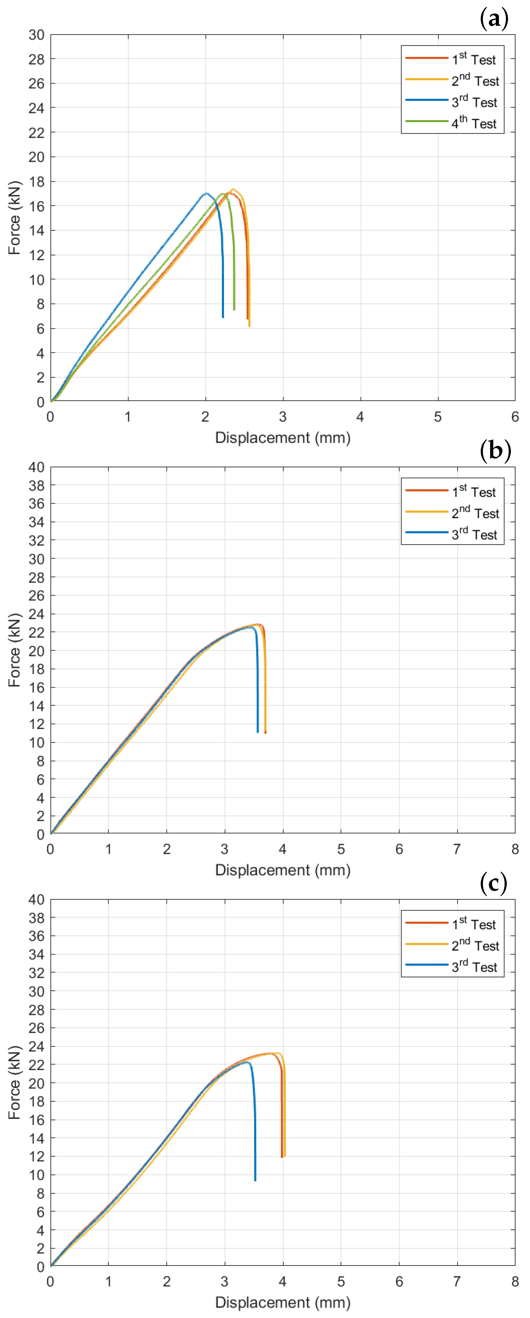
Unpatched specimens made of A36 steel with a thickness of 1/8 inch and Al 6061 with thicknesses of 1/8 inch and 0.190 inches were tested to establish the reference performance of the cracked substrates prior to patch application. Each specimen contained a central crack with a half-length of 0.145 inches. After determining the reference performance, identical cracked specimens were repaired using glass-fiber/epoxy composite patches with thicknesses of 1.0 mm and 1.64 mm and carbon-fiber/epoxy composite patches with an approximate thickness of 0.89 mm. The repaired specimens were then tested under the same loading conditions at three temperature levels: room-temperature (70 °F), high-temperature (145 °F), and low-temperature (−60 °F), to evaluate the effectiveness of the bonded patches relative to the unpatched specimens. Force–displacement curves for the unpatched, glass-fiber (GF) patched, and carbon-fiber (CF) patched Al 6061 specimens with a thickness of 1/8 inch are shown in Figure 3, while the complete set of results obtained under different environmental conditions is summarized in

Table 1. Mean critical failure loads ($P_{\mathrm{cr}}$) and standard deviations (SD) of unpatched, GF-patched, and CF-patched specimens under different temperature conditions.

Material	Temperature	Configuration	Number of Specimens, n	Mean ${\mathit{P}}_{\mathbf{cr}} \pm$ SD (kN)
Al 6061 $t=1/8^{″}$	70 °F	Unpatched	4	$17.1\pm 0.1$
		GF Patched	3	$22.7\pm 0.1$
		CF Patched	3	$22.9\pm 0.4$
	145 °F	Unpatched	3	$16.5\pm 0.2$
		GF Patched	3	$19.8\pm 0.1$
		CF Patched	3	$19.7\pm 0.1$
	−60 °F	Unpatched	3	$16.8\pm 0.0$
		GF Patched	3	$21.0\pm 0.5$
		CF Patched	3	$22.2\pm 0.6$
A36 Steel $t=1/8^{″}$	70 °F	Unpatched	3	$27.6\pm 0.4$
		GF Patched	3	$34.1\pm 0.1$
		CF Patched	3	$33.4\pm 0.4$
	145 °F	Unpatched	3	$27.6\pm 0.2$
		GF Patched	3	$27.9\pm 0.3$
		CF Patched	3	$27.5\pm 0.8$
	−60 °F	Unpatched	3	$26.9\pm 0.4$
		GF Patched	3	$31.8\pm 0.3$
		CF Patched	3	$31.8\pm 0.1$
Al 6061 $t=0.{190}^{″}$	70 °F	Unpatched	3	$25.6\pm 0.2$
		GF Patched	3	$32.4\pm 0.2$
		CF Patched	3	$32.3\pm 0.3$
	145 °F	Unpatched	3	$25.5\pm 0.2$
		GF Patched	3	$27.2\pm 0.4$
		CF Patched	3	$26.9\pm 0.3$
	−60 °F	Unpatched	3	$25.2\pm 0.2$
		GF Patched	3	$30.6\pm 0.8$
		CF Patched	3	$31.6\pm 0.2$
Al 6061 $t=0.{190}^{″}$ with thicker GF patch	70 °F	Unpatched	3	$25.6\pm 0.2$
		GF Patched	3	$33.2\pm 0.3$
	145 °F	Unpatched	3	$25.5\pm 0.2$
		GF Patched	3	$28.1\pm 0.6$
	−60 °F	Unpatched	3	$25.2\pm 0.2$
		GF Patched	3	$32.7\pm 0.1$

. Similar static tests were also performed on A36 steel unpatched, GF-patched and CF-patched specimens, with the results shown also in Table 1.

To assess the influence of adherend thickness on repair performance, tensile tests were conducted on both thin and thick Al 6061 specimens. In addition, to further investigate how increased patch thickness affects the static response of repaired aluminum structures, thick Al 6061 specimens were tested using a thicker glass-fiber/epoxy composite patch. In this configuration, 1.64 mm thick patches were used instead of 1 mm patches. These results are also summarized in Table 1. At least three specimens were tested for each configuration, and in some configurations, four specimens were tested to ensure the consistency of the experimental results. The failure loads reported in Table 1 represent the mean values obtained from the experimental tests. Since the number of specimens for each configuration was limited, standard deviations were not calculated. All experimental results were used individually in the machine learning regression model rather than being averaged.

Static tensile tests on thin and thick Al 6061 and on A36 steel specimens showed that applying bonded patches significantly improved the load-carrying capacity at room temperature, demonstrating the repair method’s effectiveness. While performance decreased at high temperature due to adhesive softening near the glass transition temperature ($T_g=63 °\mathrm{C}\approx$ 145.4 °F [36]), the repairs remained effective at low temperatures. Although the adhesive became more brittle under low-temperature conditions, the failure loads of the patched specimens were only slightly lower than those at room temperature, and no significant change in the failure mode was observed. The experimentally observed failure modes for all substrate materials, patch types, and temperature conditions are summarized in

Table 2. Summary of experimentally observed failure modes for patched specimens under different temperature conditions.

Substrate Material	Patch Type	Room (70 °F)	High (145 °F)	Low (−60 °F)
A36 Steel $t=1/8^{″}$	GF Patched	Mixed mode	Interfacial (adhesive–metal)	Interfacial (adhesive–metal)
	CF Patched	Mixed mode	Interfacial (adhesive–metal)	Interfacial (adhesive–metal)
Al 6061 $t=1/8^{″}$	GF Patched	Interfacial (adhesive–patch)	Interfacial (adhesive–metal)	Interfacial (adhesive–patch)
	CF Patched	Interfacial (adhesive–metal)	Interfacial (adhesive–metal)	Interfacial (adhesive–metal)
Al 6061 $t=0.{190}^{″}$	GF Patched	Interfacial (adhesive–metal)	Interfacial (adhesive–metal)	Interfacial (adhesive–metal)
	CF Patched	Interfacial (adhesive–metal)	Interfacial (adhesive–metal)	Interfacial (adhesive–metal)
Al 6061 $t=0.{190}^{″}$ with thicker GF patch	GF Patched	Interfacial (adhesive–patch)	Interfacial (adhesive–metal)	Interfacial (adhesive–metal)

. Representative photographs of the corresponding failure modes have been reported in our previous study [18]. This temperature-dependent behavior was consistent across all patched configurations. Increasing the patch thickness from 1 mm to 1.64 mm further improved repair efficiency, indicating that patch thickness plays an important role in overall repair performance. In contrast, changes in temperature had little effect on the unpatched specimens.

3. Finite Element Modeling of Unpatched and Patched Specimens

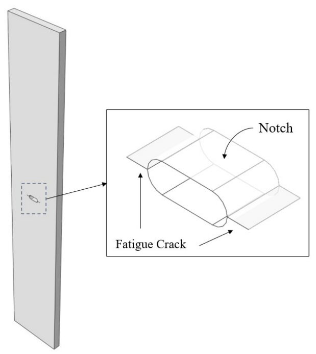
Linear finite element analyses were performed in ABAQUS©/CAE (Dassault Systèmes Simulia Corp., Johnston, RI, USA) for both unpatched and patched specimens. Separate finite element models were created for the steel and aluminum specimens to closely match the experimental setup. The main difference between the two models was the substrate thickness: Al 6061 specimens were modeled at 3.15 mm, while A36 steel specimens were modeled at 3.25 mm. These thicknesses were chosen to match the actual test specimens. Other than material properties and thickness, the geometry, loading conditions, and modeling approach were the same for both materials. The goal of these simulations was to predict the static failure loads of the patched specimens under different environmental conditions. Three-dimensional models of the specimens which included both the notch and the pre-existing crack were created, as shown in Figure 4.

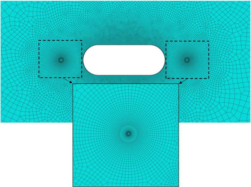
A spider mesh was generated around the crack tips to obtain an accurate stress field and properly capture the singularity, as shown in Figure 5. The crack was modeled using the seam crack option in ABAQUS©, which splits the mesh along the crack faces and allows them to open under loading. The stress intensity factors (SIFs) at the crack tips were computed using the contour integral method based on the interaction integral formulation, as implemented in ABAQUS© [37]. In this approach, the mode I and mode II stress intensity factors, ($K_I$, $K_{II}$), are directly evaluated by integrating the stress, strain, and displacement fields over a series of virtual contours surrounding the crack tip. These contours represent successive domains around the crack tip, and under linear elastic conditions, the calculated SIF values are expected to be path-independent. Therefore, three contours were used to verify convergence and ensure the numerical consistency of the results. This procedure enabled a reliable evaluation of the stress distribution near the crack tips.

The elastic properties assigned to the substrate, adhesive, and composite patch materials in the finite element model were obtained from experimental measurements and manufacturer specifications. Temperature-dependent material data were used for room temperature (70 °F), high temperature (145 °F), and low temperature (−60 °F) to incorporate thermal effects. Adhesive properties at elevated and low temperatures were taken from a previous study [36], in which butt-joint tests were performed under equivalent conditions.

The composite patches were manufactured in-house, and their elastic properties were determined experimentally.

Table 3. Properties of substrate and adhesive materials at room temperature.

Material	Elastic Modulus (GPa)	Poisson’s Ratio ($\mathit{\nu }$)
A36 Steel	200	0.26
Al 6061	68.9	0.33
Adhesive (Epoxy)	3.3	0.30

,

Table 4. Temperature-dependent elastic properties.

Material	Elastic Modulus (GPa)
	−60 °F	70 °F	145 °F
A36 Steel	202	200	197
Al 6061	70	68.9	67.5
Adhesive (Epoxy)	4.5	3.3	0.2

and

Table 5. Properties of composite patch materials.

Patch Type	${\mathit{E}}_{11}$ (GPa)	${\mathit{E}}_{22}$ (GPa)	${\mathit{E}}_{33}$ (GPa)	${\mathit{\nu }}_{12}$	${\mathit{\nu }}_{13}$	${\mathit{\nu }}_{23}$	${\mathit{G}}_{12}$ (GPa)	${\mathit{G}}_{13}$ (GPa)	${\mathit{G}}_{23}$ (GPa)
Glass-Fiber	30.3	6.3	6.3	0.29	0.29	0.33	3.0	3.0	2.4
Carbon-Fiber	141.7	5.9	5.9	0.31	0.31	0.35	1.9	1.9	2.2

provide the material parameters used in the FE analyses.

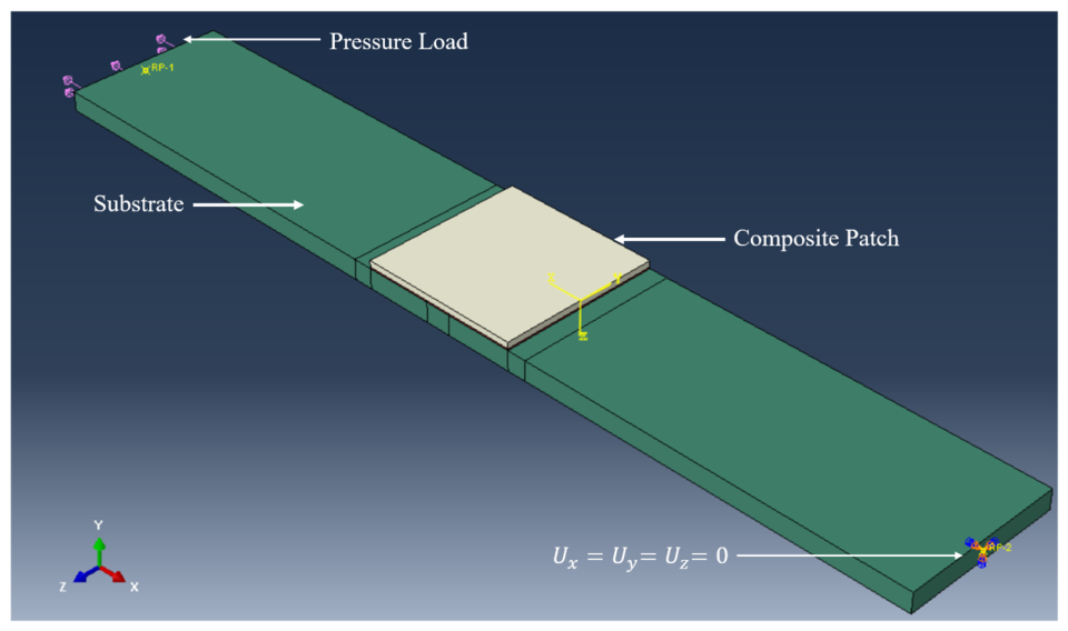
The boundary conditions applied to the patched model are shown in Figure 6. To ensure consistency, the same conditions were used for the unpatched configuration. One end was fully constrained ($Ux=Uy=Uz=0$), and a pressure load was applied to the opposite end to simulate tensile loading. The unpatched specimen’s mesh consisted of 10 elements through the thickness of the substrate, 381,029 nodes, and 340,710 C3D8R elements. In contrast, the patched model contained 873,638 nodes and 806,372 elements, comprising 772,538 C3D8R hexahedral elements and 33,834 C3D10 quadratic tetrahedral elements.

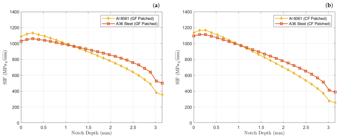
The FE analyses focused on evaluating the stress intensity factor (SIF) for a specimen with a half-crack length of 0.145 in. SIFs were extracted using the third contour, which provided stable and consistent values. Under a 20.9 kN tensile load, the SIFs and the adhesive stresses $S_{xy}$ and $S_{yy}$ were computed for glass fiber and carbon fiber patched A36 steel and Al 6061 specimens. For the patched configurations, stresses remained highest at the crack tips, with larger SIFs on the unpatched surface and reduced values on the patched side due to load redistribution. The variation of SIF through the thickness of the specimen is shown in Figure 7, where 0 mm corresponds to the unpatched surface. For both materials, the carbon-fiber patched models showed slightly lower SIF values compared to those with glass-fiber patches. This decrease is attributed to the higher stiffness of carbon fiber, which allows the patch to carry a greater share of the applied load and consequently reduces the stress intensity at the crack tip.

Finite Element Prediction of the Failure Loads of Patched Specimens

A primary objective of the finite element (FE) modeling was to determine whether the experimental failure load ($P_{\mathrm{cr}}$) of patched specimens could be predicted across various temperatures. In the thermal analyses, stress intensity factors (SIFs) resulting from temperature changes ($\Delta T$) were combined with those from mechanical loading. For simulations at −60 °F and 145 °F, $\Delta T$ was defined relative to a reference temperature of 70 °F. No external mechanical loads were applied; instead, the analyses focused on thermal stresses induced due to temperature-dependent expansion. The coefficient of thermal expansion (CTE) was defined for the metallic substrates, adhesive, and composite patches. A single isotropic CTE was used for the metals and the adhesive [38]. As unidirectional glass- and carbon-fiber composites are orthotropic, direction-dependent CTEs were required in the analyses. The longitudinal (${\alpha }_1$) and transverse (${\alpha }_2$) thermal expansion coefficients of the composite patches were calculated using the micromechanical expressions given in [39]. These equations account for the elastic moduli of the fiber ($E_f$) and matrix ($E_m$), their thermal expansion coefficients (${\alpha }_f$, ${\alpha }_m$), and their volume fractions ($V_f$, $V_m$). The longitudinal CTE, ${\alpha }_1$, was obtained using Equation (1), while the transverse CTE, ${\alpha }_2$, was determined using Equation (2). The final CTE values used in the numerical simulations are summarized in

Table 6. Thermal expansion coefficients (CTEs) for isotropic and composite materials used in the FE modeling.

(a) CTEs of Isotropic Materials
Material	CTE (${10}^{-6}\mathrm{/}°$F)
Al 6061	13.1
A36 Steel	6.5
Adhesive (Epoxy)	57
(b) Composite Fiber/Matrix Properties Used in CTE Calculations
Parameter	Value
${\alpha }_f$ (GF)	$3.1\times {10}^{-6}\mathrm{/}°$F
${\alpha }_f$ (CF)	$-0.6\times {10}^{-6}\mathrm{/}°$F
${\alpha }_m$	$37.5\times {10}^{-6}\mathrm{/}°$F
$V_f$ (GF)	0.32
$V_f$ (CF)	0.45
$V_m$ (GF)	0.68
$V_m$ (CF)	0.55
$E_f$ (GF)	85.9 GPa
$E_f$ (CF)	310.8 GPa
$E_m$ (GF)	4.1 GPa
$E_m$ (CF)	3.3 GPa
(c) CTEs of Composite Materials
Material	CTE (${10}^{-6}\mathrm{/}°$F)
Glass-fiber/epoxy (${\alpha }_1$)	6.3
Glass-fiber/epoxy (${\alpha }_2$)	40.7
Carbon-fiber/epoxy (${\alpha }_1$)	−0.1
Carbon-fiber/epoxy (${\alpha }_2$)	31.6

.

$${\alpha }_1={\displaystyle \frac{E_f{\alpha }_f{V}_f+E_m{\alpha }_m{V}_m}{E_f{V}_f+E_m{V}_m}}$$

(1)

$${\alpha }_2=(1+V_f){\alpha }_f{V}_f+(1+V_m){\alpha }_m{V}_m-{\alpha }_1(V_f^2+V_m^2)$$

(2)

Thermal-stress FE analyses were performed on Al 6061 and A36 steel specimens for both patched and unpatched configurations. For each model, the average stress intensity factors (SIFs) along the notch depth were calculated under mechanical loading and then scaled using the experimental failure load of the unpatched specimen. Assuming that failure occurs at a critical stress intensity factor, the predicted failure load for each patched configuration, ${\left(P_{cr}\right)}_{\mathrm{patched}}$, was obtained by scaling the experimental failure load of the unpatched specimen, ${\left(P_{cr}\right)}_{\mathrm{unpatched}}$, using the ratio of the stress intensity factors. In this approach, the predicted failure load was calculated as:

$${\left(P_{cr}\right)}_{\mathrm{patched}}={\left(P_{cr}\right)}_{\mathrm{unpatched}}\times {\displaystyle \frac{{\left(K_{Ic}\right)}_{\mathrm{unpatched}}}{{\left(K_I\right)}_{\mathrm{patched}}}}$$

where ${\left(K_{Ic}\right)}_{\mathrm{unpatched}}$ represents the critical stress intensity factor obtained from the finite element analysis using the failure load for the unpatched configuration, and ${\left(K_I\right)}_{\mathrm{patched}}$ represents the average stress intensity factor calculated for the patched configuration using the same load. Due to the three-dimensional effects, the highest stress intensity factor may not be located at the surface. Failure starts at the location where the stress intensity factor is the highest. However, as failure progresses, the load is redistributed, and the stress intensity factor changes accordingly. Therefore, the average stress intensity factor was used for the failure prediction.

The average stress intensity factor was calculated as the arithmetic mean of the SIF values extracted at discrete positions along the crack front:

$${\overline{K}}_I={\displaystyle \frac{1}{N}}{\displaystyle \sum _{i=1}^N}{K}_{I,i}$$

where ${\overline{K}}_I$ is the average stress intensity factor, $K_{I,i}$ is the stress intensity factor at the i-th nodal position along the crack front, and N is the number of nodal positions considered. The crack front was discretized into a finite number of elements through the specimen thickness, and the SIF at each node was extracted from the corresponding contour integral and averaged to obtain the representative through-thickness value used in the failure load predictions.

Thermal SIFs due to the applied temperature change ($\Delta T$) were combined with the mechanical SIFs through linear superposition:

$$K_{I,\mathrm{total}}=K_{I,\mathrm{mech}}\pm K_{I,\mathrm{thermal}}$$

where $K_{I,\mathrm{total}}$ is the resultant stress intensity factor used for the failure predictions, $K_{I,\mathrm{mech}}$ is the stress intensity factor obtained from the mechanical loading analysis, and $K_{I,\mathrm{thermal}}$ is the stress intensity factor obtained from the thermal analysis at the applied $\Delta T$. A sign convention was adopted in which a positive $K_{I,\mathrm{thermal}}$ corresponds to a crack-opening contribution, whereas a negative value corresponds to a crack-closing contribution. Temperature-dependent adhesive properties were included in all high- and low-temperature simulations. The resulting total SIFs for all configurations and temperatures are presented in

Table 7. Summary of experimental and FE-predicted failure loads, corresponding SIF values, and percentage errors under different temperature conditions [18].

Material and Temperature	Models	Experimental Failure Load (kN)	Reference Load for SIF ${\left({\mathit{P}}_{\mathbf{cr}}\right)}_{\mathbf{unpatched}}$ (kN)	Average SIF Along Notch Depth (MPa$\sqrt{\mathbf{mm}}$)	FE Predicted Failure Load ${\left({\mathit{P}}_{\mathbf{cr}}\right)}_{\mathbf{patched}}$ (kN)	Error
Al 6061 Room-Temperature (70 °F)	Unpatched	17.1	17.1	836.8	–	–
	GF-Patched	22.7		686.1	20.9	−8.0%
	CF-Patched	22.9		648.9	22.1	−3.5%
Al 6061 Low-Temperature (60 °F)	Unpatched	16.8	16.8	822.1	–	–
	GF-Patched	20.9		677.6	20.4	−2.4%
	CF-Patched	22.2		660.4	20.9	−5.8%
Al 6061 High-Temperature (145 °F)	Unpatched	16.5	16.5	807.4	–	–
	GF-Patched	19.7		707.8	18.8	−4.5%
	CF-Patched	19.7		690.4	19.3	−2.0%
A36 Steel Room-Temperature (70 °F)	Unpatched	27.6	27.6	1320.3	–	–
	GF-Patched	34.1		1158.7	31.5	−7.6%
	CF-Patched	33.4		1104.9	32.9	−1.5%
A36 Steel Low-Temperature (−60 °F)	Unpatched	26.8	26.8	1281.9	–	–
	GF-Patched	31.7		1116.8	30.7	−3.2%
	CF-Patched	31.8		1097.1	31.3	−1.6%
A36 Steel High-Temperature (145 °F)	Unpatched	27.6	27.6	1320.3	–	–
	GF-Patched	27.9		1209.7	30.1	+7.8%
	CF-Patched	27.5		1194.0	30.5	+10.9%

.

Using the SIFs obtained at room temperature (mechanical loading only) and under low (−60 °F) and high (145 °F) thermal conditions, the critical failure loads ($P_{\mathrm{cr}}$) were predicted for each configuration. The predicted values for Al 6061 and A36 steel specimens repaired with glass- and carbon-fiber patches are also listed in Table 7. To assess the accuracy of the FE simulations, the predicted ${\left(P_{\mathrm{cr}}\right)}_{\mathrm{patched}}$ results were compared with the experimental data, and the corresponding errors were calculated.

At room temperature, the FE predictions aligned well with the experiments, with errors ranging from −8.0% to −1.6%. Under low-temperature conditions, all predictions were within 5.8% of the experimental results. At high temperature, the deviations remained below 10.9%, with the largest being a +10.9% overprediction for the carbon-fiber patched steel specimens. At higher temperatures, adhesive softening occurs, and therefore the predicted results are less reliable. Indeed, as expected, the prediction error for some high temperature cases is larger than the error for room and low temperature cases. Both the aluminum and steel specimens showed clear improvements at room and low temperatures, while the level of improvement was lower at high temperature. Overall, the finite element model demonstrated good accuracy, with all prediction errors remaining within acceptable limits.

4. Machine Learning Models

Ten regression models were evaluated to learn the mapping from the design inputs to the static failure load: linear regression (LR), polynomial regression (PR), support vector regression (SVR), random forest (RF), gradient boosting (GB), XGBoost, LightGBM, Gaussian process (GP) regression, artificial neural networks (ANNs), and Kolmogorov–Arnold networks (KANs). A general background on ANNs can be found in [40]. Linear Regression (LR) and Polynomial Regression (PR) were included as low-capacity references that capture linear and low-order polynomial relationships between the design inputs and the failure load, respectively. Support Vector Regression (SVR) extends the margin-based formulation of support vector machines to regression by fitting a function within an $\epsilon$-insensitive tube while penalizing model complexity, making it well-suited to small datasets [41].

Tree-based ensemble models were also considered because of their robustness on small, structured datasets. Random Forest (RF) averages the predictions of many regression trees grown on bootstrap samples to reduce variance [42], whereas Gradient Boosting (GB) builds an additive ensemble in which each successive tree is fitted to the residuals of the current model in a stage-wise manner [43]. Two optimized gradient-boosting implementations were also evaluated: XGBoost, which introduces regularization and a second-order approximation of the loss to improve accuracy and efficiency [44], and LightGBM, which uses histogram-based, leaf-wise tree growth together with gradient-based one-side sampling to accelerate training [45]. In addition, Gaussian Process (GP) regression was included as a non-parametric Bayesian method that provides probabilistic predictions with associated uncertainty estimates, a feature that is attractive when the amount of physical data is limited [46].

As a novel contribution of this study, a Kolmogorov–Arnold Network (KAN) was also evaluated as a recently proposed state-of-the-art alternative to conventional multilayer perceptrons. In contrast to standard ANNs, which apply fixed activation functions at the nodes, KANs place learnable univariate activation functions, parametrized as splines, on the network edges, following the Kolmogorov–Arnold representation theorem [47]. This formulation enables compact networks to represent complex nonlinear mappings with improved data efficiency and interpretability, which is particularly relevant to the limited-data regime of bonded patch repair. To the best of the authors’ knowledge, KANs have not previously been applied to predicting the static performance of bonded structural patch repairs.

4.1. Model Implementation and Hyperparameter Selection

All regression models were implemented in Python. The classical and ensemble baselines (LR, PR, SVR, RF, GB, GP) were implemented in scikit-learn [48], using the dedicated XGBoost and LightGBM libraries for the two boosted-tree models, while the ANN and the KAN were implemented in PyTorch, with the KAN built on the pykan library of the original authors [47]. For every regression model, the hyperparameters were tuned by grid search inside the inner grouped cross-validation loop; the configuration with the lowest inner cross-validated error was retained, and its performance was then estimated on the corresponding outer folds, which were never used for selection. Because the outer folds serve only for evaluation, the reported error is an unbiased nested estimate rather than a hold-out that also informed the model choice. The search space explored for each model is summarized in

Table 8. Hyperparameter search space explored for each model.

Model	Hyperparameter Search Space
Linear Regression	None (ordinary least squares).
Polynomial Regression	Polynomial degree $\in \{2,3\}$; ridge penalty $\alpha \in \{0.1,1,10\}$.
Support Vector Regression	RBF kernel; $C\in \{1,10,100\}$; $\epsilon \in \{0.1,0.5\}$.
Random Forest	Number of trees $\in \{100,200,300\}$; maximum depth $\in \{\mathrm{None},10,20\}$; minimum samples per split $\in \{2,5\}$.
Gradient Boosting	Number of trees $\in \{100,200\}$; maximum depth $\in \{2,3\}$; learning rate $\in \{0.05,0.1\}$.
XGBoost	Number of trees $\in \{100,200,300\}$; maximum depth $\in \{3,6\}$; learning rate $\in \{0.05,0.1\}$.
LightGBM	Number of trees $\in \{100,200,300\}$; maximum depth $\in \{-1,10\}$; learning rate $\in \{0.05,0.1\}$.
Gaussian Process	RBF + white-noise kernel; length scale $1.0$; noise level $\in \{0.1,1.0\}$; $\alpha ={10}^{-6}$.
KAN	Width $[n_{\mathrm{in}},16,1]$; grid size 5; spline order 3; learning rate $0.01$.
ANN (this study)	Architectures: [32, 16, 8], [64, 32, 16], [64, 32, 16, 8], [128, 64, 32], [128, 64, 32, 16, 8]; activation functions: ReLU, Leaky ReLU, ELU, tanh, SELU; learning rate $0.001$; dropout rate $\in \{0.0,0.1\}$.

, and the resulting accuracies are compared in

Table 9. Comparison of regression models under configuration-grouped nested cross-validation (real data only; mean absolute percentage error ± standard deviation across outer folds, and mean $R^2$). Models are sorted by patched MAPE; the best model per dataset is in bold.

	Patched		Unpatched
Model	MAPE (%)	${\mathbf{R}}^{\mathbf{2}}$	MAPE (%)	${\mathbf{R}}^{\mathbf{2}}$
Gradient Boosting	2.78 ± 0.65	0.873	7.08 ± 1.14	0.917
Random Forest	2.89 ± 0.36	0.846	13.31 ± 3.23	0.776
XGBoost	2.97 ± 0.71	0.867	6.88 ± 2.12	0.905
KAN	3.23 ± 0.90	0.889	6.68 ± 3.00	0.941
Gaussian Process	5.08 ± 2.44	0.779	3.33 ± 0.76	0.983
Linear Regression	7.41 ± 1.28	0.017	11.23 ± 3.98	0.900
Polynomial Regression	8.17 ± 5.15	0.196	4.35 ± 2.44	0.976
LightGBM	8.82 ± 3.31	0.422	15.75 ± 4.43	0.726
ANN (this study)	8.90 ± 4.29	−0.03	10.30 ± 5.75	0.881
Support Vector Regression	10.34 ± 8.49	0.106	7.04 ± 2.16	0.938

. The mean absolute percentage error (MAPE) was used as the main performance metric for all regression models; the ANN and KAN were trained with the Adam optimizer and the mean squared error (MSE) loss.

For the ANN, the architecture refers to the topology of the hidden layers, i.e., the number of hidden layers and the number of neurons in each, whereas the remaining hyperparameters are the activation function, the learning rate that scales the weight updates at each epoch, and the dropout rate. Five hidden-layer topologies were evaluated:

• [32, 16, 8]—three hidden layers (56 neurons)
• [64, 32, 16]—three hidden layers (112 neurons)
• [64, 32, 16, 8]—four hidden layers (120 neurons)
• [128, 64, 32]—three hidden layers (224 neurons)
• [128, 64, 32, 16, 8]—five hidden layers (248 neurons)

These topologies were combined with five activation functions (ReLU, Leaky ReLU, ELU, tanh, and SELU), a learning rate of 0.001, and two dropout rates (0.0 and 0.1), giving a total of 50 distinct ANN configurations. ANN training used a batch size of 16, a maximum of 400 epochs, and early stopping with a patience of 30 epochs to mitigate overfitting.

The baseline models were tuned over standard ranges (Table 8). SVR used an RBF kernel, with the penalty parameter C and the $\epsilon$-tube width as the primary tuning parameters. The tree ensembles (RF, GB, XGBoost, and LightGBM) were tuned over the number of trees, the maximum tree depth, and, for the boosted variants, the learning rate. The GP regressor used a squared-exponential (RBF) kernel combined with a white-noise term whose level was tuned. The KAN used a compact width of $[n_{\mathrm{in}}, 16, 1]$ with cubic B-splines (spline order 3) on a grid of size 5 and a learning rate of 0.01; because pykan training is markedly slower than the ANN, its grid was deliberately kept small.

4.2. Computational Environment

All regression-model training and nested cross-validation were performed on a Dell XPS 15 9520 laptop (Intel Core i7-12700H, 14 physical cores/20 threads, up to 4.7 GHz; 64 GB RAM) running Pop!_OS 22.04 (Linux kernel 7.0.9). The pipeline was implemented in Python 3.10 using scikit-learn 1.7.2, XGBoost 3.1.3, LightGBM 4.6.0, PyTorch 2.9.1, pandas 2.3.3, and NumPy 2.2.6.

5. Data Collection and Preprocessing

All regression models were trained and evaluated under a leakage-free, configuration-grouped protocol. Only real samples (experimental, finite-element, and theoretical) define the ground truth, and GMM synthetic data are confined to the training partition of each fold. Because several specimens share the same physical configuration, the data were grouped by unique configuration (material, thicknesses, temperature, and patch type): all replicates and the finite-element/theoretical points belonging to a configuration are always kept together in the same fold, so no configuration appears simultaneously in a training and an evaluation partition. Model family, hyperparameters, preprocessing, and augmentation are selected within an inner cross-validation loop, and performance is reported from an outer loop that is never used for any selection. The reported error therefore reflects generalization to unseen configurations rather than specimen-to-specimen scatter.

5.1. Dataset Composition

The datasets were combined from three sources: $\left(i\right)$ experimental results, $\left(ii\right)$ theoretical failure load predictions for the unpatched specimens and finite element (FE) predictions for the patched specimens, and $\left(iii\right)$ synthetic samples generated with a Gaussian Mixture Model (GMM) to enlarge the training data, as described in Section 5.2. Each real sample carries a provenance label, so the datasets are traceable. The patched baseline contains 75 real samples (63 experimental and 12 FE), and the unpatched baseline contains 72 real samples (27 experimental and 45 theoretical). Because several specimens share the same material–thickness–temperature–patch configuration, the real data were grouped by unique physical configuration (21 configurations for the patched dataset and 54 for the unpatched dataset), and all replicates together with the associated finite-element/theoretical points of a configuration were always assigned to the same fold. Evaluation used nested grouped cross-validation, with an outer GroupKFold loop (five folds) for unbiased performance estimation and an inner GroupKFold loop (three folds) for model and hyperparameter selection. GMM synthetic samples were added only inside the training partition of each fold, enlarging that pool to 300 samples during model development, whereas every validation and outer-evaluation partition contained only real data.

5.1.1. Dataset of Unpatched Specimens

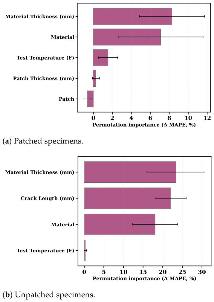
The unpatched baseline of 72 real samples was expanded to 300 samples by adding 228 synthetic samples (Section 5.2). The model inputs are the Material Type (A36 steel or Al 6061), the Crack Length (mm), the Test Temperature (°F), and the Material Thickness (mm), while the output is the Failure Load (kN). Material Type is a categorical (text) input, whereas the remaining inputs and the output are numerical. As a feature-engineering step, the categorical input was one-hot encoded and the numerical inputs were standardized before training [48]. The permutation-importance analysis (Figure 8) was carried out within the configuration-grouped framework: for every outer fold the increase in MAPE ($\Delta$MAPE) caused by randomly permuting each input was measured on the held-out configurations and averaged over 50 permutations, and the mean and standard deviation were then aggregated across folds. It indicates that the failure load of the unpatched specimens is driven almost entirely by the material thickness ($\Delta$MAPE $\approx 23\%$), the crack length (≈$22\%$), and the material type (≈$17\%$)—together roughly $99\%$ of the total importance—whereas the test temperature has negligible direct effect ($\Delta$MAPE $<0.5\%$) [42]; these three inputs are therefore the main drivers of an accurate prediction. The theoretical failure loads used here were obtained from the mode I stress intensity factor ($K_I$) for a uniformly loaded strip containing an internal crack [49].

5.1.2. Dataset of Patched Specimens

The patched baseline of 75 real samples (experimental data and FE predictions) was expanded to 300 samples by adding 225 synthetic samples (Section 5.2). The model inputs are the Material Type, the Material Thickness (mm), the Patch Material, the Patch Thickness (mm), and the Test Temperature (°F), while the output is the Failure Load (kN). Material Type and Patch Material are categorical inputs, whereas the others and the output are numerical. As for the unpatched case, the categorical inputs were one-hot encoded, and the numerical inputs were standardized before training [48]. The permutation-importance analysis (Figure 8), computed with the same grouped, uncertainty-aware procedure, shows that the patched failure load is governed mainly by the substrate thickness ($\Delta$MAPE $\approx 8$–$9\%$) and the material type (≈7–$8\%$), which together account for roughly 85–$90\%$ of the importance, followed by the test temperature (≈1–$3\%$) and, to a negligible extent, the patch thickness and patch type [42]. The standard deviations across folds (shown as error bars in Figure 8) are appreciable, reflecting the small number of patched configurations, so these rankings should be read as indicative rather than exact. These trends are consistent with the experimental observations and support the use of the regression models within the tested envelope (Al 6061/A36 steel, $-60$ to 145 °F).

5.2. Synthetic Data Generation

Because physical testing is costly and time-consuming, a Gaussian Mixture Model (GMM) was used to oversample the cross-validation training folds. The GMM assumes that the data are drawn from a mixture of several Gaussian distributions and estimates the joint distribution of the inputs and the output, so that new, statistically representative samples can be drawn [50]. In this study, the GMM used a full covariance structure with three mixture components; a small number of components was chosen deliberately to avoid over-fitting the mixture on the limited baseline (75 and 72 real samples), and the Bayesian information criterion was monitored across one to five components as a consistency check. Each augmented training fold was enlarged to 300 samples.

To keep the synthetic data from biasing the evaluation, the leakage-free, configuration-grouped protocol in Section 5 was applied as follows. Only the real samples (experimental, finite-element, and theoretical) were treated as ground truth. The real data were split by unique physical configuration using nested grouped cross-validation; within each training partition, the GMM was fit to that partition only and used to augment it, while the corresponding validation and outer-evaluation partitions contained only real data and never shared a configuration with the training partition. Because the GMM is fit to the joint distribution and the sampled inputs are subsequently clipped to the physical range and snapped to admissible design values, the generated failure load is not re-derived from the snapped inputs; the synthetic samples are therefore used only to enlarge the training folds and are never used as ground truth for validation or testing. This separation ensures that no synthetic sample and no configuration leaks across folds, and it prevents the optimistic bias that would otherwise arise.

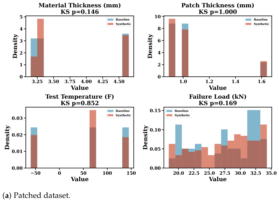
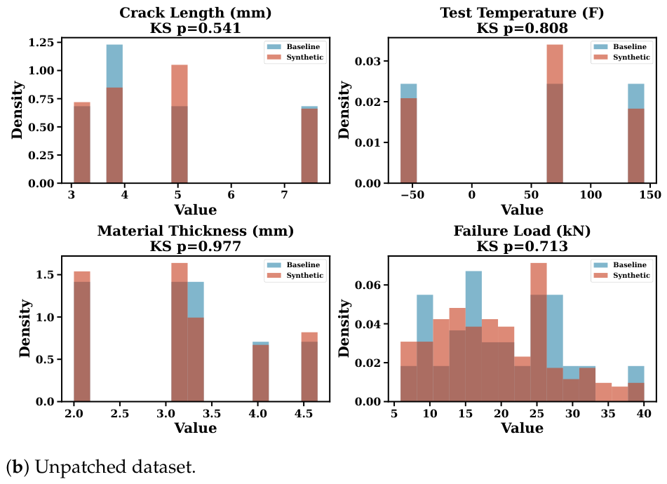
The quality of the synthetic data was checked with the Kolmogorov–Smirnov (KS) test, which compares the distribution of each generated feature with that of the original data [51]. The generation followed an acceptance protocol: the categorical inputs were sampled jointly with the numerical variables and decoded onto the existing classes only, the numerical values were clipped to the physical range observed in the baseline, and the near-discrete design inputs (such as the test temperature and the patch thickness) were snapped to their valid values. Sampling used a fixed random seed and was repeated for up to five attempts until all features passed the KS test at the 5% significance level. For both datasets, an admissible set passing all KS tests was obtained on the first attempt (rejection rate of 0 out of the five permitted retries), with only a small difference in the correlation structure between the synthetic and the original data (0.13 for the patched and 0.15 for the unpatched dataset). Figure 9 overlays the baseline and synthetic distributions of the numerical variables for both datasets, together with the per-feature KS p-values. The close overlap between the two distributions confirms that the synthetic samples reproduce the marginal distributions of the real data while remaining within physically admissible ranges. Because marginal KS tests alone do not guarantee that conditional relationships are preserved, the generated failure-load distribution was additionally compared with the baseline within each material and patch class, and the sign of its correlation with each numerical input was checked; these class-conditional comparisons remained consistent with the baseline, indicating that the dominant physical trends were retained. The influence of the number of synthetic samples on model accuracy is examined in Section 6 as part of the augmentation assessment.

5.3. Preprocessing

Prior to training, the categorical inputs (Material and Patch) were one-hot encoded, so that each category is represented by a binary indicator vector and no artificial ordering is introduced among the classes. The numerical inputs were standardized using a StandardScaler. To prevent information leakage, the scaler, the encoder, and the GMM generator were fit only on the training partition of each grouped cross-validation fold [48,52]. For each outer fold, the held-out configurations were transformed using a preprocessor fitted only to the (augmented) outer-training pool, and they were never included in model selection or hyperparameter tuning.

6. Results and Discussion

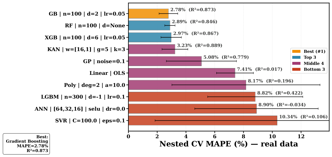
The regression models were evaluated under the configuration-grouped, leakage-free protocol described in Section 5: for every model the hyperparameters were selected inside an inner GroupKFold loop, and the accuracy was estimated on the outer folds, which were never used for selection. Because the data are grouped by unique physical configuration, this measures the ability to predict unseen configurations rather than replicate-to-replicate scatter. Unless stated otherwise, the reported metrics are the models trained on the real data only (experimental, FE, and theoretical); the effect of adding GMM synthetic samples is analyzed separately in Section 6.4. Table 9, the bar charts in Figures 10 and 12, and the scatter plots in Figures 11 and 13 report the nested-CV metrics for the best configuration of each model. Selection-CV results for the full 116-configuration search space are provided in the Appendix A (

Table A1. Full grouped selection cross-validation results for every configuration evaluated (patched dataset). Values are 5-fold GroupKFold metrics (GMM-augmented training folds) used for hyperparameter selection, not the nested test estimate.

Configuration	CV MAPE (%)	CV ${\mathit{R}}^2$
Linear Regression
None (OLS)	7.35 ± 1.24	−0.287
Polynomial Regression
degree 2, $\alpha$ = 10	9.15 ± 4.75	−0.925
degree 2, $\alpha$ = 1	9.18 ± 5.47	−0.892
degree 3, $\alpha$ = 10	10.95 ± 5.67	−1.293
degree 3, $\alpha$ = 1	12.09 ± 5.55	−2.361
degree 2, $\alpha$ = 0.1	12.59 ± 11.22	−1.272
degree 3, $\alpha$ = 0.1	12.86 ± 5.90	−2.999
Support Vector Regression
RBF kernel, C = 100, $\epsilon$ = 0.1	10.80 ± 5.45	−1.152
RBF kernel, C = 10, $\epsilon$ = 0.1	10.89 ± 4.93	−0.785
RBF kernel, C = 100, $\epsilon$ = 0.5	10.98 ± 5.18	−1.088
RBF kernel, C = 10, $\epsilon$ = 0.5	11.34 ± 4.73	−0.889
RBF kernel, C = 1, $\epsilon$ = 0.5	12.44 ± 6.27	−1.471
RBF kernel, C = 1, $\epsilon$ = 0.1	12.56 ± 5.96	−1.606
Random Forest
100 trees, depth None, min. split 2	11.06 ± 6.27	−1.085
100 trees, depth 20, min. split 2	11.06 ± 6.27	−1.085
100 trees, depth 10, min. split 2	11.06 ± 6.27	−1.085
100 trees, depth 10, min. split 5	11.06 ± 6.26	−1.082
100 trees, depth 20, min. split 5	11.06 ± 6.26	−1.082
100 trees, depth None, min. split 5	11.06 ± 6.26	−1.082
300 trees, depth None, min. split 2	11.22 ± 6.57	−1.040
300 trees, depth 10, min. split 2	11.22 ± 6.57	−1.040
300 trees, depth 20, min. split 2	11.22 ± 6.57	−1.040
300 trees, depth 10, min. split 5	11.24 ± 6.61	−1.037
300 trees, depth 20, min. split 5	11.24 ± 6.61	−1.037
300 trees, depth None, min. split 5	11.24 ± 6.61	−1.037
200 trees, depth None, min. split 5	11.32 ± 6.67	−1.105
200 trees, depth 10, min. split 5	11.32 ± 6.67	−1.105
200 trees, depth 20, min. split 5	11.32 ± 6.67	−1.105
200 trees, depth 20, min. split 2	11.32 ± 6.68	−1.109
200 trees, depth 10, min. split 2	11.32 ± 6.68	−1.109
200 trees, depth None, min. split 2	11.32 ± 6.68	−1.109
Gradient Boosting
100 trees, depth 2, lr 0.05	8.97 ± 5.44	−0.202
200 trees, depth 2, lr 0.05	9.17 ± 4.94	−0.326
100 trees, depth 2, lr 0.1	10.66 ± 7.75	−0.538
200 trees, depth 2, lr 0.1	10.72 ± 7.50	−0.655
100 trees, depth 3, lr 0.1	11.84 ± 7.87	−1.019
200 trees, depth 3, lr 0.1	11.91 ± 7.95	−1.087
100 trees, depth 3, lr 0.05	12.27 ± 8.89	−0.991
200 trees, depth 3, lr 0.05	12.41 ± 9.04	−1.095
XGBoost
100 trees, depth 6, lr 0.05	8.10 ± 3.21	−0.894
300 trees, depth 6, lr 0.1	8.15 ± 3.09	−0.904
200 trees, depth 6, lr 0.1	8.15 ± 3.09	−0.904
100 trees, depth 6, lr 0.1	8.15 ± 3.10	−0.904
200 trees, depth 6, lr 0.05	8.18 ± 3.12	−0.903
300 trees, depth 6, lr 0.05	8.20 ± 3.13	−0.905
100 trees, depth 3, lr 0.05	8.66 ± 2.98	−0.675
300 trees, depth 3, lr 0.05	8.92 ± 3.04	−0.829
200 trees, depth 3, lr 0.05	8.94 ± 3.01	−0.805
100 trees, depth 3, lr 0.1	8.97 ± 3.10	−0.808
200 trees, depth 3, lr 0.1	9.02 ± 3.11	−0.807
300 trees, depth 3, lr 0.1	9.12 ± 3.17	−0.818
LightGBM
300 trees, depth −1, lr 0.1	10.52 ± 5.85	−0.942
300 trees, depth 10, lr 0.1	10.52 ± 5.85	−0.942
300 trees, depth 10, lr 0.05	10.54 ± 6.00	−0.884
300 trees, depth −1, lr 0.05	10.54 ± 6.00	−0.884
200 trees, depth −1, lr 0.1	10.55 ± 6.00	−0.923
200 trees, depth 10, lr 0.1	10.55 ± 6.00	−0.923
200 trees, depth 10, lr 0.05	10.62 ± 6.05	−0.854
200 trees, depth −1, lr 0.05	10.62 ± 6.05	−0.854
100 trees, depth 10, lr 0.1	10.63 ± 6.10	−0.878
100 trees, depth −1, lr 0.1	10.63 ± 6.10	−0.878
100 trees, depth 10, lr 0.05	10.70 ± 6.15	−0.741
100 trees, depth −1, lr 0.05	10.70 ± 6.15	−0.741
Gaussian Process
RBF + white kernel, noise 0.1	8.27 ± 2.37	−0.649
RBF + white kernel, noise 1	8.27 ± 2.37	−0.649
KAN
width [16,1], grid 5, order 3, lr 0.01	8.68 ± 2.35	−0.599
ANN (this study)
[64,32,16], SELU, lr 0.001, dropout 0	7.01 ± 1.81	−0.216
[128,64,32], ELU, lr 0.001, dropout 0.1	7.34 ± 1.25	−0.132
[128,64,32,16,8], ELU, lr 0.001, dropout 0	7.40 ± 1.00	−0.364
[64,32,16], ELU, lr 0.001, dropout 0	7.51 ± 1.65	−0.329
[128,64,32], ELU, lr 0.001, dropout 0	7.53 ± 0.91	−0.380
[32,16,8], SELU, lr 0.001, dropout 0	7.59 ± 2.38	−0.160
[128,64,32], SELU, lr 0.001, dropout 0.1	7.69 ± 1.67	−0.265
[64,32,16,8], SELU, lr 0.001, dropout 0	7.72 ± 2.02	−0.362
[32,16,8], SELU, lr 0.001, dropout 0.1	7.73 ± 1.83	−0.773
[64,32,16], SELU, lr 0.001, dropout 0.1	7.79 ± 2.29	−0.255
[64,32,16,8], SELU, lr 0.001, dropout 0.1	7.82 ± 1.92	−1.214
[64,32,16,8], ELU, lr 0.001, dropout 0.1	7.85 ± 1.46	−0.968
[64,32,16,8], ELU, lr 0.001, dropout 0	7.87 ± 1.95	−0.330
[32,16,8], ELU, lr 0.001, dropout 0	7.88 ± 2.17	−0.221
[128,64,32,16,8], SELU, lr 0.001, dropout 0	7.91 ± 2.37	−0.256
[128,64,32], SELU, lr 0.001, dropout 0	7.98 ± 2.69	−0.280
[64,32,16], ELU, lr 0.001, dropout 0.1	8.04 ± 1.76	−0.280
[32,16,8], ELU, lr 0.001, dropout 0.1	8.14 ± 1.99	−0.843
[128,64,32,16,8], SELU, lr 0.001, dropout 0.1	8.19 ± 3.02	−0.267
[128,64,32,16,8], ELU, lr 0.001, dropout 0.1	8.27 ± 2.09	−0.241
[32,16,8], Leaky ReLU, lr 0.001, dropout 0	8.42 ± 1.57	−0.632
[32,16,8], Leaky ReLU, lr 0.001, dropout 0.1	8.69 ± 1.83	−0.775
[32,16,8], ReLU, lr 0.001, dropout 0	8.93 ± 1.38	−0.858
[128,64,32,16,8], Leaky ReLU, lr 0.001, dropout 0	9.02 ± 1.43	−0.445
[128,64,32], Leaky ReLU, lr 0.001, dropout 0.1	9.08 ± 1.19	−0.935
[64,32,16], Leaky ReLU, lr 0.001, dropout 0	9.14 ± 1.31	−0.567
[128,64,32], Leaky ReLU, lr 0.001, dropout 0	9.24 ± 1.73	−0.491
[64,32,16,8], Leaky ReLU, lr 0.001, dropout 0.1	9.42 ± 1.26	−0.909
[32,16,8], ReLU, lr 0.001, dropout 0.1	9.46 ± 1.41	−1.844
[128,64,32,16,8], Leaky ReLU, lr 0.001, dropout 0.1	9.67 ± 2.12	−0.852
[64,32,16], ReLU, lr 0.001, dropout 0	9.71 ± 1.71	−0.528
[128,64,32], ReLU, lr 0.001, dropout 0.1	9.84 ± 1.61	−0.568
[64,32,16,8], ReLU, lr 0.001, dropout 0	9.85 ± 1.55	−0.781
[128,64,32], ReLU, lr 0.001, dropout 0	10.03 ± 1.89	−0.573
[64,32,16,8], Leaky ReLU, lr 0.001, dropout 0	10.19 ± 2.35	−0.814
[64,32,16,8], ReLU, lr 0.001, dropout 0.1	10.20 ± 1.63	−1.377
[64,32,16], ReLU, lr 0.001, dropout 0.1	10.28 ± 1.83	−1.234
[64,32,16], Leaky ReLU, lr 0.001, dropout 0.1	10.29 ± 1.94	−1.189
[128,64,32,16,8], ReLU, lr 0.001, dropout 0	10.58 ± 1.41	−0.779
[128,64,32,16,8], ReLU, lr 0.001, dropout 0.1	11.14 ± 1.75	−1.305
[128,64,32], Tanh, lr 0.001, dropout 0.1	17.19 ± 8.23	−5.427
[64,32,16], Tanh, lr 0.001, dropout 0	17.24 ± 8.13	−5.416
[128,64,32], Tanh, lr 0.001, dropout 0	17.35 ± 7.98	−5.466
[64,32,16], Tanh, lr 0.001, dropout 0.1	18.30 ± 6.99	−5.570
[64,32,16,8], Tanh, lr 0.001, dropout 0	18.31 ± 7.03	−5.557
[128,64,32,16,8], Tanh, lr 0.001, dropout 0	18.31 ± 7.01	−5.573
[32,16,8], Tanh, lr 0.001, dropout 0	18.31 ± 7.02	−5.559
[64,32,16,8], Tanh, lr 0.001, dropout 0.1	18.38 ± 7.01	−5.577
[128,64,32,16,8], Tanh, lr 0.001, dropout 0.1	18.39 ± 7.02	−5.578
[32,16,8], Tanh, lr 0.001, dropout 0.1	18.39 ± 7.01	−5.572

and 

Table A2. Full grouped selection cross-validation results for every configuration evaluated (unpatched dataset). Values are 5-fold GroupKFold metrics (GMM-augmented training folds) used for hyperparameter selection, not the nested test estimate.

Configuration	CV MAPE (%)	CV ${\mathit{R}}^2$
Linear Regression
None (OLS)	11.80 ± 2.97	0.873
Polynomial Regression
degree 2, $\alpha$ = 0.1	7.51 ± 1.44	0.931
degree 2, $\alpha$ = 1	7.53 ± 1.41	0.930
degree 2, $\alpha$ = 10	8.09 ± 1.40	0.925
degree 3, $\alpha$ = 10	11.08 ± 2.80	0.848
degree 3, $\alpha$ = 1	12.04 ± 3.62	0.791
degree 3, $\alpha$ = 0.1	12.28 ± 3.84	0.780
Support Vector Regression
RBF kernel, C = 10, $\epsilon$ = 0.1	8.52 ± 0.72	0.925
RBF kernel, C = 10, $\epsilon$ = 0.5	8.77 ± 0.81	0.922
RBF kernel, C = 100, $\epsilon$ = 0.1	11.03 ± 1.75	0.865
RBF kernel, C = 100, $\epsilon$ = 0.5	11.46 ± 2.20	0.864
RBF kernel, C = 1, $\epsilon$ = 0.1	12.83 ± 2.08	0.862
RBF kernel, C = 1, $\epsilon$ = 0.5	13.03 ± 2.05	0.858
Random Forest
200 trees, depth None, min. split 5	10.17 ± 2.75	0.868
200 trees, depth 10, min. split 5	10.17 ± 2.75	0.868
200 trees, depth 20, min. split 5	10.17 ± 2.75	0.868
300 trees, depth None, min. split 5	10.20 ± 2.72	0.869
300 trees, depth 10, min. split 5	10.20 ± 2.72	0.869
300 trees, depth 20, min. split 5	10.20 ± 2.72	0.869
100 trees, depth None, min. split 5	10.34 ± 2.78	0.860
100 trees, depth 10, min. split 5	10.34 ± 2.78	0.860
100 trees, depth 20, min. split 5	10.34 ± 2.78	0.860
200 trees, depth None, min. split 2	10.62 ± 2.29	0.869
200 trees, depth 10, min. split 2	10.62 ± 2.29	0.869
200 trees, depth 20, min. split 2	10.62 ± 2.29	0.869
300 trees, depth None, min. split 2	10.68 ± 2.23	0.870
300 trees, depth 20, min. split 2	10.68 ± 2.23	0.870
300 trees, depth 10, min. split 2	10.68 ± 2.23	0.870
100 trees, depth 20, min. split 2	10.71 ± 2.33	0.862
100 trees, depth 10, min. split 2	10.71 ± 2.33	0.862
100 trees, depth None, min. split 2	10.71 ± 2.33	0.862
Gradient Boosting
200 trees, depth 2, lr 0.1	9.02 ± 2.66	0.880
100 trees, depth 2, lr 0.1	9.64 ± 2.86	0.861
200 trees, depth 2, lr 0.05	9.69 ± 3.03	0.856
100 trees, depth 3, lr 0.1	10.19 ± 4.56	0.823
200 trees, depth 3, lr 0.05	10.33 ± 4.45	0.823
100 trees, depth 2, lr 0.05	10.55 ± 3.06	0.831
100 trees, depth 3, lr 0.05	10.61 ± 4.22	0.824
200 trees, depth 3, lr 0.1	10.86 ± 4.57	0.807
XGBoost
100 trees, depth 3, lr 0.1	10.07 ± 4.26	0.822
200 trees, depth 3, lr 0.05	10.22 ± 4.45	0.822
300 trees, depth 3, lr 0.05	10.70 ± 4.23	0.818
100 trees, depth 3, lr 0.05	10.73 ± 4.21	0.822
200 trees, depth 3, lr 0.1	11.00 ± 4.16	0.815
300 trees, depth 3, lr 0.1	11.38 ± 4.24	0.813
100 trees, depth 6, lr 0.05	12.38 ± 3.22	0.824
200 trees, depth 6, lr 0.05	12.93 ± 3.44	0.810
100 trees, depth 6, lr 0.1	13.03 ± 2.86	0.808
300 trees, depth 6, lr 0.05	13.13 ± 3.49	0.807
200 trees, depth 6, lr 0.1	13.38 ± 2.91	0.800
300 trees, depth 6, lr 0.1	13.41 ± 2.91	0.800
LightGBM
200 trees, depth −1, lr 0.05	10.58 ± 2.65	0.857
200 trees, depth 10, lr 0.05	10.58 ± 2.65	0.857
100 trees, depth −1, lr 0.05	10.64 ± 2.66	0.855
100 trees, depth 10, lr 0.05	10.64 ± 2.66	0.855
100 trees, depth −1, lr 0.1	10.94 ± 3.00	0.847
100 trees, depth 10, lr 0.1	10.94 ± 3.00	0.847
300 trees, depth 10, lr 0.05	11.02 ± 3.13	0.846
300 trees, depth −1, lr 0.05	11.02 ± 3.13	0.846
200 trees, depth 10, lr 0.1	11.29 ± 3.55	0.837
200 trees, depth −1, lr 0.1	11.29 ± 3.55	0.837
300 trees, depth −1, lr 0.1	11.57 ± 3.42	0.827
300 trees, depth 10, lr 0.1	11.57 ± 3.42	0.827
Gaussian Process
RBF + white kernel, noise 1	6.97 ± 1.88	0.933
RBF + white kernel, noise 0.1	6.97 ± 1.88	0.933
KAN
width [16,1], grid 5, order 3, lr 0.01	8.41 ± 2.16	0.899
ANN (this study)
[64,32,16], SELU, lr 0.001, dropout 0.1	5.51 ± 1.03	0.961
[64,32,16], SELU, lr 0.001, dropout 0	5.64 ± 1.15	0.958
[64,32,16,8], SELU, lr 0.001, dropout 0	5.78 ± 1.07	0.952
[64,32,16,8], SELU, lr 0.001, dropout 0.1	5.90 ± 1.77	0.953
[32,16,8], SELU, lr 0.001, dropout 0	5.92 ± 1.46	0.951
[32,16,8], SELU, lr 0.001, dropout 0.1	5.96 ± 1.26	0.945
[32,16,8], ELU, lr 0.001, dropout 0.1	6.22 ± 1.19	0.942
[128,64,32], SELU, lr 0.001, dropout 0.1	6.49 ± 1.49	0.949
[64,32,16], ELU, lr 0.001, dropout 0.1	6.52 ± 1.57	0.948
[128,64,32], SELU, lr 0.001, dropout 0	6.63 ± 1.76	0.947
[64,32,16], ELU, lr 0.001, dropout 0	6.67 ± 1.70	0.943
[32,16,8], ELU, lr 0.001, dropout 0	6.72 ± 1.74	0.940
[128,64,32,16,8], SELU, lr 0.001, dropout 0	6.74 ± 2.24	0.930
[64,32,16,8], ELU, lr 0.001, dropout 0.1	6.79 ± 1.60	0.943
[128,64,32,16,8], ELU, lr 0.001, dropout 0	6.82 ± 2.19	0.934
[128,64,32], ELU, lr 0.001, dropout 0	6.90 ± 1.72	0.939
[64,32,16,8], ELU, lr 0.001, dropout 0	7.02 ± 2.10	0.931
[128,64,32], ELU, lr 0.001, dropout 0.1	7.15 ± 1.64	0.937
[128,64,32,16,8], ELU, lr 0.001, dropout 0.1	7.19 ± 1.25	0.945
[128,64,32,16,8], SELU, lr 0.001, dropout 0.1	7.20 ± 1.72	0.943
[128,64,32,16,8], Leaky ReLU, lr 0.001, dropout 0	7.84 ± 2.31	0.915
[128,64,32,16,8], Leaky ReLU, lr 0.001, dropout 0.1	8.09 ± 2.78	0.905
[32,16,8], ReLU, lr 0.001, dropout 0	8.21 ± 2.77	0.913
[128,64,32], Leaky ReLU, lr 0.001, dropout 0	8.28 ± 2.17	0.913
[128,64,32], Leaky ReLU, lr 0.001, dropout 0.1	8.34 ± 2.07	0.912
[64,32,16,8], Leaky ReLU, lr 0.001, dropout 0	8.78 ± 2.32	0.902
[32,16,8], Leaky ReLU, lr 0.001, dropout 0.1	8.81 ± 1.32	0.911
[128,64,32,16,8], ReLU, lr 0.001, dropout 0	8.85 ± 2.10	0.900
[64,32,16], ReLU, lr 0.001, dropout 0	8.86 ± 2.27	0.905
[32,16,8], ReLU, lr 0.001, dropout 0.1	8.98 ± 2.63	0.901
[64,32,16], Leaky ReLU, lr 0.001, dropout 0.1	9.05 ± 2.32	0.899
[128,64,32], ReLU, lr 0.001, dropout 0.1	9.11 ± 2.45	0.894
[64,32,16], Leaky ReLU, lr 0.001, dropout 0	9.12 ± 2.50	0.901
[64,32,16,8], ReLU, lr 0.001, dropout 0.1	9.17 ± 2.33	0.901
[32,16,8], Leaky ReLU, lr 0.001, dropout 0	9.26 ± 2.09	0.900
[64,32,16], Tanh, lr 0.001, dropout 0.1	9.28 ± 1.53	0.873
[64,32,16,8], Leaky ReLU, lr 0.001, dropout 0.1	9.30 ± 3.10	0.895
[128,64,32,16,8], ReLU, lr 0.001, dropout 0.1	9.56 ± 2.31	0.890
[64,32,16,8], ReLU, lr 0.001, dropout 0	9.61 ± 2.35	0.889
[128,64,32], ReLU, lr 0.001, dropout 0	9.86 ± 2.02	0.889
[64,32,16], ReLU, lr 0.001, dropout 0.1	9.86 ± 2.80	0.886
[64,32,16], Tanh, lr 0.001, dropout 0	9.88 ± 2.82	0.849
[32,16,8], Tanh, lr 0.001, dropout 0	9.93 ± 2.56	0.843
[128,64,32], Tanh, lr 0.001, dropout 0.1	10.24 ± 1.62	0.861
[32,16,8], Tanh, lr 0.001, dropout 0.1	10.76 ± 3.96	0.801
[128,64,32], Tanh, lr 0.001, dropout 0	10.92 ± 2.19	0.852
[64,32,16,8], Tanh, lr 0.001, dropout 0.1	11.08 ± 5.64	0.796
[64,32,16,8], Tanh, lr 0.001, dropout 0	30.24 ± 16.74	0.203
[128,64,32,16,8], Tanh, lr 0.001, dropout 0.1	46.18 ± 10.84	−0.154
[128,64,32,16,8], Tanh, lr 0.001, dropout 0	46.73 ± 11.16	−0.161

).

6.1. Patched Specimen Predictions

On the real hold-out test set, Support Vector Regression (SVR) achieved the lowest error (MAPE 3.73%, $R^2$ 0.937), followed closely by LightGBM (MAPE 4.24%, $R^2$ 0.919), KAN (MAPE 4.59%, $R^2$ 0.911), and Random Forest (MAPE 4.64%, $R^2$ 0.907). The selected ANN ([128, 64, 32, 16, 8], Leaky ReLU, learning rate 0.001, no dropout) reached a hold-out MAPE of 5.81% and $R^2$ of 0.874, indicating that the ANN remains competitive although it was not the top performer on the patched dataset.

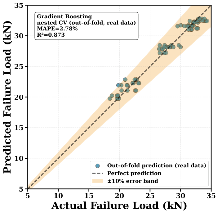
Figure 10 ranks the ten models by nested-CV MAPE and confirms that the tree ensembles (Gradient Boosting, Random Forest, XGBoost) and the KAN are the most accurate, while the linear/kernel baselines and the ANN show the largest errors. The out-of-fold scatter plot in Figure 11 shows that most real points fall within the ±10% band for the best model (Gradient Boosting).

6.2. Unpatched Specimen Predictions

For the unpatched specimens, XGBoost delivered the best hold-out accuracy (MAPE 3.18%, $R^2$ 0.994), with Gradient Boosting (MAPE 4.48%, $R^2$ 0.984) and Random Forest (MAPE 4.56%, $R^2$ 0.988) also performing strongly. The selected ANN ([64, 32, 16], SELU, learning rate 0.001, no dropout) attained a hold-out MAPE of 5.37% and $R^2$ of 0.981. Although the unpatched ANN shows a higher $R^2$ than the patched ANN, this reflects the greater variance of the unpatched failure loads rather than a lower relative error.

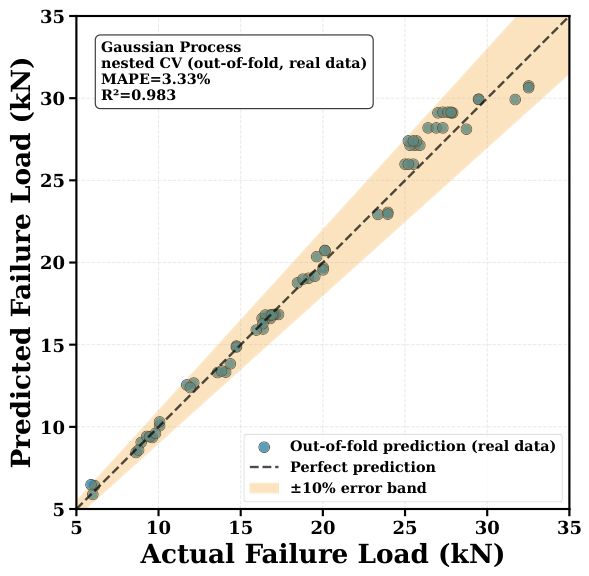
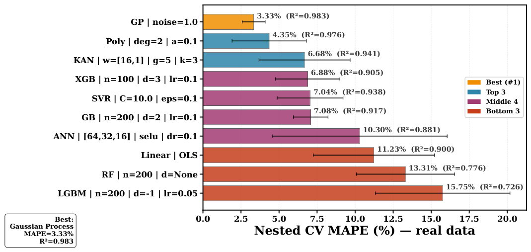
Figure 12 shows that XGBoost achieved the lowest hold-out error, with the other tree-ensemble models also in the top group, whereas linear regression performed poorly. The hold-out scatter plot in Figure 13 shows a close agreement with the perfect-prediction line for the same best model (XGBoost), with most points within the ±10% band.

6.3. Comparison and Practical Implications

Table 9 compares all regression models on the real hold-out test set (sorted by patched hold-out MAPE). For the patched specimens, classical and ensemble regressors (especially SVR and LightGBM) matched or exceeded the ANN, whereas for the unpatched specimens, XGBoost and the other tree ensembles were the most accurate. The KAN, included as a state-of-the-art alternative, performed competitively on the patched dataset (4.59% MAPE) but was less accurate on the unpatched case (8.25% MAPE). Overall, the results indicate that the FE-augmented, leakage-free framework supports reliable failure-load prediction within the tested design space, while the optimal regressor depends on the dataset, and no single model dominated both cases.

Table 10. Best regression model for each dataset under configuration-grouped nested cross-validation, with the real-data-only and GMM-augmented estimates.

Parameter	Patched Dataset	Unpatched Dataset
Best model	Gradient Boosting	Gaussian Process
Hyperparameters	100 trees, depth 2, learning rate 0.05	RBF + white kernel, noise level $1.0$
Real-only nested MAPE (%)	2.78 ± 0.65	3.33 ± 0.76
Real-only nested $R^2$	0.873	0.983
+GMM nested MAPE (%)	8.97 ± 5.44	6.97 ± 1.88
+GMM nested $R^2$	−0.20	0.933
Augmentation effect (p)	$+6.19$ ($p=0.08$)	$+3.63$ ($p=0.01$)

summarizes the best-performing model for each dataset, reporting both the real-data-only nested estimate and the estimate obtained when GMM-synthesized samples are added to the training folds (the augmentation effect is analyzed in Section 6.4). The patched top performer (Gradient Boosting, $2.78\%$ MAPE) corresponds to an average absolute error of approximately $0.78$ kN on a mean failure load of $28.22$ kN, whereas the unpatched top performer (Gaussian Process, $3.33\%$ MAPE) corresponds to approximately $0.64$ kN on a mean of $19.17$ kN.

6.4. Effect of GMM Synthetic Augmentation

Because the reduced-order rationale for this study is that synthetic data can compensate for a scarce experimental dataset, the benefit of the GMM augmentation was tested explicitly rather than assumed. For every model the same nested procedure was run twice on identical outer folds—once with the real data only and once with GMM synthetic samples added to the (inner and outer) training partitions—and the two errors were compared with a paired t-test across the five outer folds. Since only five paired differences are available for each model, we treat these p-values as exploratory and read them together with the fold-wise error differences and standard deviations, rather than as definitive evidence of statistical significance.

Table 11. Effect of GMM synthetic augmentation on the nested-CV MAPE (%). “Real” uses experimental, FE, and theoretical data only; “+GMM” adds GMM-synthesized training samples. A positive $\Delta$ means augmentation increases the error. ^∗ marks a paired difference with $p<0.05$ across the five outer folds; given the small number of folds, these p-values are exploratory and should be read together with the reported error differences.

	Patched			Unpatched
Model	Real	+GMM	$\Delta$	Real	+GMM	$\Delta$
Gradient Boosting	2.78	8.97	$+6.19$	7.08	9.81	$+2.73$
Random Forest	2.89	11.12	$+8.24$	13.31	10.13	−3.18 ∗
XGBoost	2.97	8.66	+5.68 ∗	6.88	10.60	$+3.72$
KAN	3.23	8.68	+5.45 ∗	6.68	8.41	$+1.73$
Gaussian Process	5.08	8.27	$+3.20$	3.33	6.97	+3.63 ∗
Linear Regression	7.41	7.36	$-0.05$	11.23	11.80	$+0.57$
Polynomial Regression	8.17	9.81	$+1.64$	4.35	7.79	$+3.44$
LightGBM	8.82	10.47	$+1.65$	15.75	10.98	$-4.77$
ANN (this study)	8.90	7.94	$-0.96$	10.30	7.13	$-3.17$
Support Vector Reg.	10.34	11.45	$+1.11$	7.04	8.75	$+1.71$

lists the resulting nested MAPE for both settings.

For the most accurate regressors on each dataset—gradient boosting (patched) and the Gaussian process (unpatched)—adding GMM samples clearly degraded accuracy. Several models (XGBoost and KAN on the patched data, and the Gaussian process on the unpatched data) reached $p<0.05$, but with only five paired folds these values are exploratory; the consistent, often several-percent increases in MAPE are what primarily support this conclusion rather than the tests themselves. Augmentation improved the error only for models that were already poor (e.g., Random Forest and the ANN on the unpatched data), and never turned a weak model into a competitive one. This behavior was confirmed by a sensitivity analysis in which the synthetic sample count was varied: for the unpatched Gaussian process the nested MAPE rose monotonically from $3.33\%$ with no synthetic data to $6.37\%$, $6.97\%$, and $8.36\%$ as the training pool was expanded to 150, 300, and 600 samples, respectively; the patched case showed no benefit at any synthetic count. We therefore report the real-data models as the primary result and retain the GMM pipeline as a documented—but, for these datasets, unhelpful—augmentation strategy. A likely explanation is that the GMM, fitted to only a few dozen configurations, reproduces the marginal and low-order conditional statistics of the data (Section 5.2) but not the sharp physical relationship between the design variables and the failure load, so the added samples act as mild noise for the stronger learners while modestly regularizing the weaker ones.

7. Conclusions

The experimental results showed that bonded composite patch repairs effectively improved the load-carrying capacity of both Al 6061 and A36 steel specimens under room and low-temperature conditions. Although the effectiveness of the repairs decreased at elevated temperatures due to adhesive softening, both glass-fiber and carbon-fiber patches provided improvements of a similar order over the unpatched specimens. Given the small number of replicates per configuration, this observation is based on the measured means and their scatter rather than on a formal statistical test, and it should be read as an indication that the two patch types performed comparably under the conditions investigated, not as a proof of statistical equivalence. In addition, increasing patch thickness further enhanced repair performance, indicating its beneficial effect within the tested range.

To complement the experimental investigation, machine-learning regression models were developed to predict the static failure loads ($P_{\mathrm{cr}}$) of unpatched specimens and specimens repaired with glass- or carbon-fiber composite patches under varying temperature conditions. Although the available experimental dataset was limited, combining the experimental measurements with finite element (FE) predictions and closed-form theoretical estimates provided a multi-source real dataset from which the regression models could learn the underlying temperature-dependent behavior with good accuracy.

Under a strict, configuration-grouped nested cross-validation—in which whole physical configurations, rather than individual specimens, are held out, and hyperparameters are selected on inner folds that are never used for evaluation—the best regression models achieved MAPE values of $2.78\%$ (Gradient Boosting, patched specimens, $R^2=0.87$) and $3.33\%$ (Gaussian Process, unpatched specimens, $R^2=0.98$) on entirely unseen configurations. Compact, lower-variance learners (tree ensembles, Gaussian process, polynomial regression, and KAN) generalized best, whereas higher-capacity models such as the ANN tended to overfit these small grouped datasets. Contrary to our initial expectation, adding GMM-synthesized samples did not improve accuracy: it left the best models unchanged or, more often, degraded them (with consistent, often several-percent increases in MAPE), so the reported models use the real, multi-source data only, and the GMM pipeline is retained as a documented but—for these datasets—unhelpful augmentation strategy.

These findings indicate the potential of machine-learning regression models for predicting static failure loads within the tested design space, while also clarifying the boundaries of that claim. Several limitations should be emphasized. First, the datasets are small (21 patched and 54 unpatched configurations); the wide fold-to-fold scatter and the near-zero $R^2$ of some patched models show that predicting genuinely unseen configurations remains difficult, and the reported errors should be read together with their standard deviations. Second, a substantial fraction of the training targets are FE and closed-form theoretical values, so the models partly learn those physics-based surrogates rather than experiments alone. Third, the models interpolate within the investigated envelope—Al 6061 and A36 steel substrates, temperatures from −60 °F to 145 °F, substrate thicknesses of 1/8 inch (3.18 mm) and 0.190 inch (4.83 mm), and patch thicknesses between 1.0 mm and 1.64 mm—and should not be expected to extrapolate to untested materials, temperatures, or patch configurations. Broader validation on additional experiments therefore remains necessary before general predictive reliability can be claimed. Overall, the proposed FE-augmented machine-learning framework provides an efficient, rigorously validated complement to experimental testing for the static performance of bonded composite patch repairs within the investigated design space.

References

1. Mohammadi, S.; Yousefi, M.; Khazaei, M. A review on composite patch repairs and the most important parameters affecting its efficiency and durability. J. Reinf. Plast. Compos. 2020, 40, 3–15. [Google Scholar] [CrossRef] [Scilit]
2. Schubbe, J.J. Thickness Effects on a Cracked Aluminum Plate with Composite Patch Repair. Ph.D. Thesis, Air Force Institute of Technology, Dayton, OH, USA, 1997. [Google Scholar]
3. Tavakkolizadeh, M.; Saadatmanesh, H. Fatigue Strength of Steel Girders Strengthened with Carbon Fiber Reinforced Polymer Patch. J. Struct. Eng.-ASCE 2003, 129. [Google Scholar] [CrossRef] [Scilit]
4. Jones, R.; Chiu, W. Composite Repairs to Cracks in Thick Metallic Components. Compos. Struct. 1999, 44, 17–29. [Google Scholar] [CrossRef] [Scilit]
5. Jones, R. Repair of Multi-site Damage. In Advances in the Bonded Composite Repair of Metallic Aircraft Structure; Springer: Berlin/Heidelberg, Germany, 2002; pp. 375–402. [Google Scholar]
6. Baker, A.; Callinan, R.; Davis, M.; Jones, R.; Williams, J. Repair of mirage III aircraft using the BFRP crack-patching technique. Theor. Appl. Fract. Mech. 1984, 2, 1–15. [Google Scholar] [CrossRef] [Scilit]
7. Hosseini-Toudeshky, H.; Sadeghi, G.; Daghyani, H. Experimental fatigue crack growth and crack-front shape analysis of asymmetric repaired aluminium panels with glass/epoxy composite patches. Compos. Struct. 2005, 71, 401–406. [Google Scholar] [CrossRef] [Scilit]
8. Mohammed, S.M.A.K.; Essaheb, M. Effect of Patch Thickness on the Repair Performance of Bonded Composite Repair in Cracked Aluminum Plate. Mater. Today Proc. 2017, 4, 9020–9028. [Google Scholar] [CrossRef] [Scilit]
9. Xiong, J.J.; Shenoi, R.A. Integrated Experimental Screening of Bonded Composite Patch Repair Schemes to Notched Aluminum-Alloy Panels Based on Static and Fatigue Strength Concepts. Compos. Struct. 2008, 83, 266–272. [Google Scholar] [CrossRef] [Scilit]
10. Broek, D.; Schijve, J. The Influence of Sheet Thickness on Crack Propagation: An investigation into the effect of sheet thickness on the propagation of fatigue cracks in 2024-T3 alclad sheet material. Aircr. Eng. 1966, 38, 31–33. [Google Scholar] [CrossRef] [Scilit]
11. Kan, H.P.; Ratwani, M. Composite Patch Repair of Cracked Thick Aluminum Structures. In Proceedings of the 25th Structures, Structural Dynamics and Materials Conference, Palm Springs, CA, USA, 14–16 May 1984; AIAA: Reston, VA, USA, 1984. [Google Scholar]
12. Srilakshmi, R. Experimental and Numerical Investigation of Adhesively Bonded Composite Patch Repair of an Inclined Center Cracked Aluminium Panel under Static and Fatigue Load; Technical Report; Indian Institute of Technology Hyderabad: Kandi, India, 2014. [Google Scholar]
13. Srilakshmi, R.; Ramji, M.; Chinthapenta, V. Fatigue crack growth study of CFRP patch repaired Al 2014-T6 panel having an inclined center crack using FEA and DIC. Eng. Fract. Mech. 2015, 134, 182–201. [Google Scholar] [CrossRef] [Scilit]
14. Liu, H.; Al-Mahaidi, R.; Zhao, X.L. Experimental study of fatigue crack growth behavior in adhesively reinforced steel structures. Compos. Struct. 2009, 90, 12–20. [Google Scholar] [CrossRef] [Scilit]
15. Li, L.; Chen, T.; Zhang, N.; Hidekuma, Y. Test on fatigue repair of central inclined cracked steel plates using different adhesives and CFRP, prestressed and non prestressed. Compos. Struct. 2019, 216, 350–359. [Google Scholar] [CrossRef] [Scilit]
16. Günther, G.; Maier, A. Composite Repair for Metallic Aircraft Structures: Development and Qualification Aspects. In Proceedings of the 27th International Congress of the Aeronautical Sciences (ICAS 2010), European Aeronautic Defense and Space Company (EADS), Nice, France, 19–24 September 2010; Military Air Systems: Nice, France, 2010. [Google Scholar]
17. Kokner, Y. An Environmental and Durability Study of Bonded Structural Patch Repairs with Finite Element and Machine Learning Enabled Predictions. Ph.D. Thesis, The City College of New York, New York, NY, USA, 2025. ProQuest No. 32237989. [Google Scholar]
18. Kokner, Y.; Delale, F.; Elvin, N. Effect of temperature on the static response of bonded structural patch repairs. Int. J. Adhes. Adhes. 2026, 147, 104279. [Google Scholar] [CrossRef] [Scilit]
19. Papanikos, P.; Tserpes, K.; Pantelakis, S. Initiation and progression of composite patch debonding in adhesively repaired cracked metallic sheets. Compos. Struct. 2007, 81, 303–311. [Google Scholar] [CrossRef] [Scilit]
20. Bouiadjra, B.B.; Belhouari, M.; Serier, B. Computation of the stress intensity factors for repaired cracks with bonded composite patch in mode I and mixed mode. Compos. Struct. 2002, 56, 401–406. [Google Scholar] [CrossRef] [Scilit]
21. Gunes, R.; Armanios, E.A. Fracture mechanics analysis of cracked aircraft structural components repaired by composite patches. Compos. Struct. 2002, 58, 207–213. [Google Scholar]
22. Achour, T.; Bouiadjra, B.B.; Serier, B. Numerical analysis of the performances of the bonded composite patch for reducing stress concentration and repairing cracks at notch. Comput. Mater. Sci. 2003, 28, 41–48. [Google Scholar] [CrossRef] [Scilit]
23. Walde, S.S.; Lilhare, S. Finite Element Analysis of Composite Patch Repaired Cracked Metal Plates and Effect of Patch Thickness on SIF. Int. J. Eng. Res. Technol. 2016, 4, 43–46. [Google Scholar] [CrossRef] [Scilit]
24. Belhouari, M.; Bouiadjra, B.B.; Achour, B.; Serier, B. Comparison of double and single bonded repairs to symmetric composite structures: A numerical analysis. Compos. Struct. 2004, 65, 47–53. [Google Scholar] [CrossRef] [Scilit]
25. Ouinas, D.; Bouiadjra, B.B.; Belhouari, M.; Achour, B.; Serier, B. Comparison of the effectiveness of boron/epoxy and graphite/epoxy patches for repaired cracks emanating from a semicircular notch edge. J. Reinf. Plast. Compos. 2007, 26, 1803–1816. [Google Scholar]
26. Kumar, M.; Singh, R. 3D Finite Element Modelling of Composite Patch Repair. In Proceedings of the International Conference on Fracture, Sydney, Australia, 1–5 April 1997. [Google Scholar] [CrossRef] [Scilit]
27. Alkunte, S.; Fidan, I. Machine Learning-Based Fatigue Life Prediction of Functionally Graded Materials Using Material Extrusion Technology. J. Compos. Sci. 2023, 7, 420. [Google Scholar] [CrossRef] [Scilit]
28. Magliacano, D.; Letizia, A.; Di Palo, S.; Alecci, M.; Bazzani, M. Element-level finite-element-informed machine-learning surrogates for failure-index prediction in a composite wing box with intralaminar damage. Aerosp. Sci. Technol. 2026, 177, 112878. [Google Scholar] [CrossRef] [Scilit]
29. Rohman, M.N.; Hidayat, M.I.P.; Purniawan, A. Prediction of Composite Fatigue Life under Variable Amplitude Loading Using Artificial Neural Network Trained by Genetic Algorithm. In Proceedings of the AIP Conference Proceedings, Tamil Nadu, India, 27–28 September 2018; Volume 1945, p. 020019. [Google Scholar] [CrossRef] [Scilit]
30. Vassilopoulos, A.P.; Georgopoulos, C.E.; Dionysopoulos, D. Modelling fatigue life of multidirectional GFRP laminates under constant amplitude loading with artificial neural networks. J. Strain Anal. Eng. Des. 2006, 41, 159–167. [Google Scholar]
31. El Kadi, H. Fatigue life prediction of composite materials: Artificial neural networks vs. polynomial classifiers. Key Eng. Mater. 2011, 471–472, 221–226. [Google Scholar] [CrossRef] [Scilit]
32. Mishra, P.C.; Brahma, B.; Dutta, M. Low cycle fatigue life prediction of Al–Si–Mg alloy using artificial neural network approach. Trans. Indian Inst. Met. 2016, 69, 365–372. [Google Scholar] [CrossRef] [Scilit]
33. Suman, S.; Dwivedi, K.; Anand, S.; Pathak, H. XFEM–ANN approach to predict the fatigue performance of a composite patch repaired aluminium panel. Compos. Part C Open Access 2022, 9, 100326. [Google Scholar] [CrossRef] [Scilit]
34. Mortazavi, S.N.S.; Ince, A. Artificial neural networks-based J-integral prediction for cracked bodies under elasto-plastic deformation state—Monotonic loading. Int. J. Fatigue 2023, 167, 107311. [Google Scholar] [CrossRef] [Scilit]
35. Bahrami, B.; Talebi, H.; Ayatollahi, M.R.; Khosravani, M.R. Artificial neural network in prediction of mixed-mode I/II fracture load. Int. J. Mech. Sci. 2023, 248, 108214. [Google Scholar] [CrossRef] [Scilit]
36. Delale, F. Characterization of Adhesive Materials Under Very High Strain Rate Loading: Final Report; Technical Report NAMC Project No. 69-201511; The City College of New York, US Army—TARDEC: New York, NY, USA, 2019. [Google Scholar]
37. Dassault Systèmes. ABAQUS Analysis User’s Guide; Section: Contour Integral Evaluation; Dassault Systèmes: Vélizy-Villacoublay, France, 2023. [Google Scholar]
38. Callister, W.D.; Rethwisch, D.G. Materials Science and Engineering: An Introduction, 10th ed.; Wiley: New York, NY, USA, 2020. [Google Scholar]
39. Johnson, R.R.; Kural, M.H.; Mackey, G.B. Thermal Expansion Properties of Composite Materials; NASA Contractor Report CR-165632; Lockheed Missiles & Space Co., Inc.: Sunnyvale, CA, USA, 1981. [Google Scholar]
40. Uyar, M.U. Machine Learning and AI with Simple Python and Matlab Scripts: Courseware for Non-Computing Majors; John Wiley & Sons: Hoboken, NJ, USA, 2025. [Google Scholar]
41. Drucker, H.; Burges, C.J.; Kaufman, L.; Smola, A.; Vapnik, V. Support vector regression machines. Adv. Neural Inf. Process. Syst. 1996, 9, 155–161. [Google Scholar]
42. Breiman, L. Random forests. Mach. Learn. 2001, 45, 5–32. [Google Scholar] [CrossRef] [Scilit]
43. Friedman, J.H. Greedy function approximation: A gradient boosting machine. Ann. Stat. 2001, 29, 1189–1232. [Google Scholar] [CrossRef] [Scilit]
44. Chen, T.; Guestrin, C. Xgboost: A scalable tree boosting system. In Proceedings of the 22nd Acm Sigkdd International Conference on Knowledge Discovery and Data Mining, San Francisco, CA, USA, 13–17 August 2016; pp. 785–794. [Google Scholar]
45. Ke, G.; Meng, Q.; Finley, T.; Wang, T.; Chen, W.; Ma, W.; Ye, Q.; Liu, T.Y. Lightgbm: A highly efficient gradient boosting decision tree. Adv. Neural Inf. Process. Syst. 2017, 30, 3149–3157. [Google Scholar]
46. Seeger, M. Gaussian processes for machine learning. Int. J. Neural Syst. 2004, 14, 69–106. [Google Scholar] [CrossRef] [Scilit] [PubMed]
47. Liu, Z.; Wang, Y.; Vaidya, S.; Ruehle, F.; Halverson, J.; Soljacic, M.; Hou, T.; Tegmark, M. KAN: Kolmogorov–arnold networks. In Proceedings of the International Conference on Learning Representations, Singapore, 24–28 April 2025; Volume 2025, pp. 70367–70413. [Google Scholar]
48. Pedregosa, F.; Varoquaux, G.; Gramfort, A.; Michel, V.; Thirion, B.; Grisel, O.; Blondel, M.; Prettenhofer, P.; Weiss, R.; Dubourg, V.; et al. Scikit-learn: Machine learning in Python. J. Mach. Learn. Res. 2011, 12, 2825–2830. [Google Scholar]
49. Erdogan, F. Fracture Mechanics; Technical Report; Lehigh University: Bethlehem, PA, USA, 1975. [Google Scholar]
50. Chokwitthaya, C.; Zhu, Y.; Mukhopadhyay, S.; Jafari, A. Applying the Gaussian mixture model to generate large synthetic data from a small data set. In Proceedings of the Construction Research Congress, Reston, VA, USA, 8–10 March 2020; American Society of Civil Engineers: Reston, VA, USA, 2020; pp. 1251–1260. [Google Scholar]
51. An, K. Sulla determinazione empirica di una legge didistribuzione. Giorn Dell’inst Ital Degli Att 1933, 4, 89–91. [Google Scholar]
52. Schober, P.; Mascha, E.J.; Vetter, T.R. Statistics from A (agreement) to Z (z score): A guide to interpreting common measures of association, agreement, diagnostic accuracy, effect size, heterogeneity, and reliability in medical research. Anesth. Analg. 2021, 133, 1633–1641. [Google Scholar] [CrossRef] [Scilit] [PubMed]
Figure 1. Schematic representation of the unpatched specimens, showing (a) the overall geometry, (b) the notch and fatigue crack region, and (c) detailed dimensions of the notch geometry.
Jcs 10 00412 g001
Figure 2. Schematic of the patched specimen subjected to tensile loading. The composite patch is bonded over the crack region in the substrate. The inset shows the fiber orientation and the crack length (2a) within the patched area.
Jcs 10 00412 g002
Figure 3. Force–displacement curves for Al 6061 specimens with 1/8-inch thickness tested at room temperature: (a) unpatched specimen, (b) GF-patched specimen, (c) CF-patched specimen.
Jcs 10 00412 g003
Figure 4. FE model of the unpatched specimen, with an inset showing the notch and fatigue crack.
Jcs 10 00412 g004
Figure 5. Finite element mesh showing the spider mesh around the crack tips. The inset shows a detailed view of the crack tip region.
Jcs 10 00412 g005
Figure 6. Patched specimen configuration and boundary conditions.
Jcs 10 00412 g006
Figure 7. SIF variation along the notch depth for patched specimens: (a) GF patched (b) CF patched [18].
Jcs 10 00412 g007
Figure 8. Permutation feature importance ( Δ MAPE in the original input space, mean ± standard deviation over the outer grouped folds and 50 permutations per fold) for the patched and unpatched datasets.
Jcs 10 00412 g008
Figure 9. Baseline versus GMM-generated synthetic distributions of the numerical variables, with the per-feature Kolmogorov–Smirnov p-values, for the (a) patched and (b) unpatched datasets.
Jcs 10 00412 g009aJcs 10 00412 g009b
Figure 10. Nested cross-validation MAPE (real data) for patched specimens: all ten regression models ranked by error (best configuration per model). Error bars denote the standard deviation across the outer folds.
Jcs 10 00412 g010
Figure 11. Out-of-fold nested-CV predictions of the best-performing model (Gradient Boosting) for patched specimens: actual versus predicted failure load (MAPE 2.78 % , R 2 = 0.873 ). The dashed line represents perfect prediction, and the shaded region indicates a ±10% error band.
Jcs 10 00412 g011
Figure 12. Nested cross-validation MAPE (real data) for unpatched specimens: all ten regression models ranked by error (best configuration per model). Error bars denote the standard deviation across the outer folds.
Jcs 10 00412 g012
Figure 13. Out-of-fold nested-CV predictions of the best-performing model (Gaussian Process) for unpatched specimens: actual versus predicted failure load (MAPE 3.33 % , R 2 = 0.983 ). The dashed line represents perfect prediction, and the shaded region indicates a ±10% error band.
Jcs 10 00412 g013