


An Unsupervised Moving Object Detection Network for UAV Videos
Abstract
1. Introduction
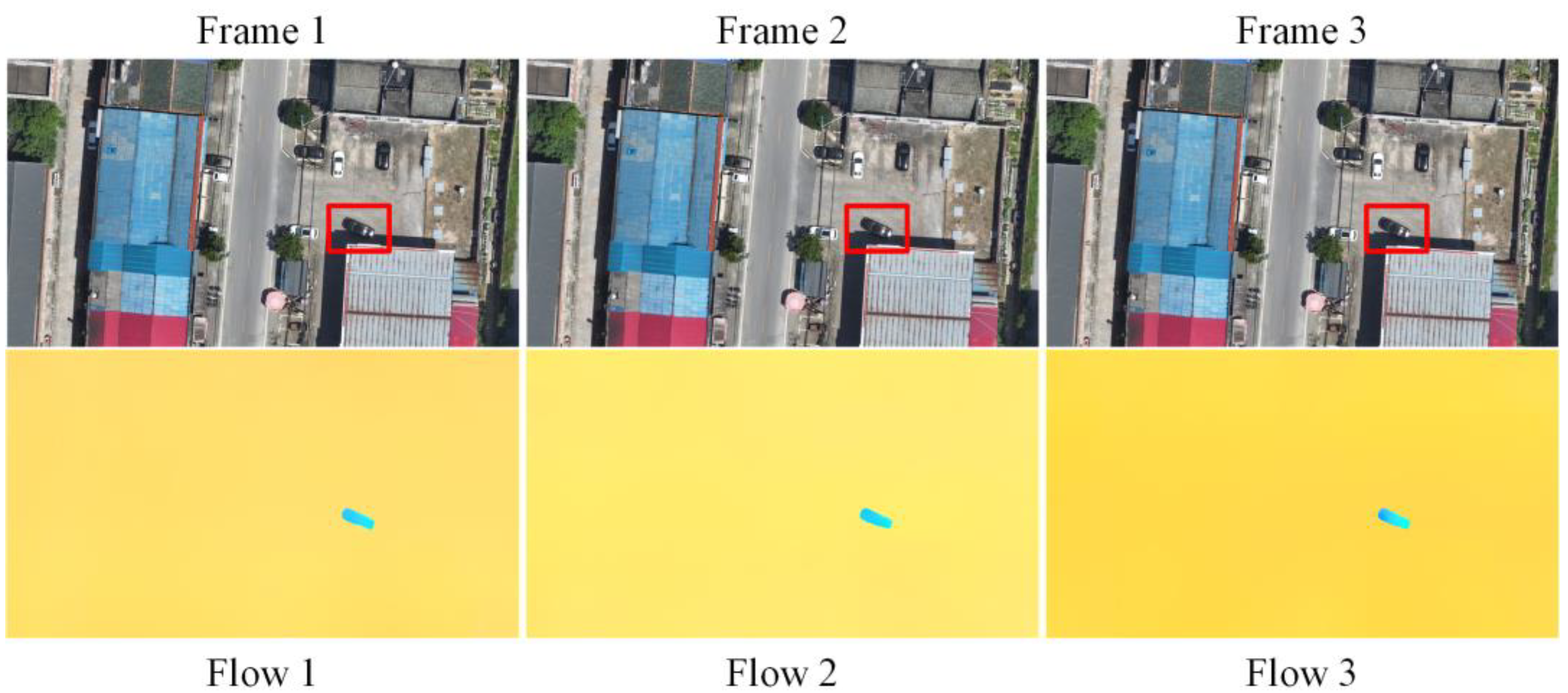
- We propose an unsupervised multi-scale UAV moving object detection network based on optical flow, which fully leverages prior knowledge in UAV scenarios. This architecture effectively separates the foreground from background by exploiting motion pattern disparities, enabling accurate detection of prominent moving objects in UAV videos.
- We incorporate prior knowledge of foreground sparsity and spatial consistency in UAV ground observation scenes using the Ising model into the loss function of the unsupervised network. This crucial step significantly mitigates false alarms arising from motion parallax and platform motion.
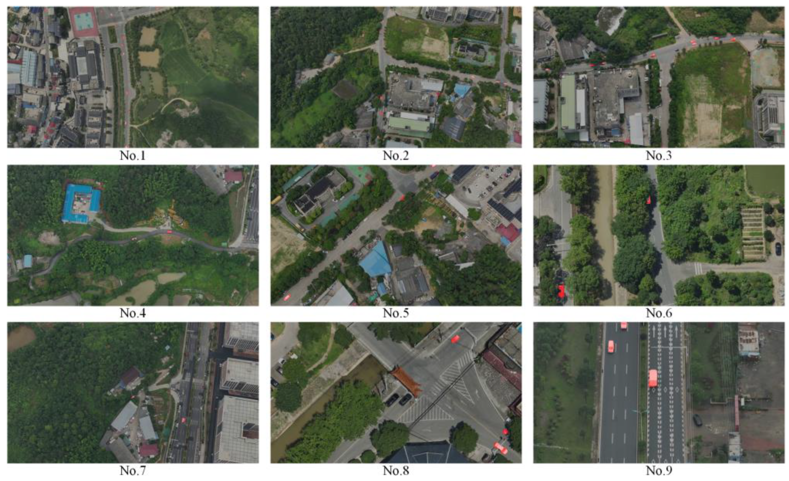
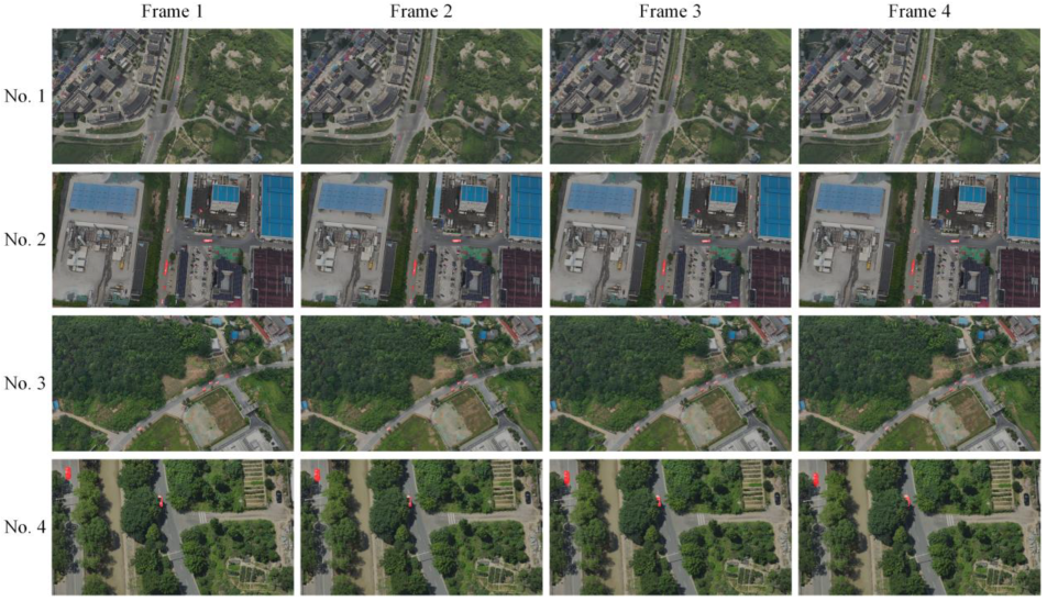
- We collected high-definition UAV-to-ground observation data using DJI drones, comprising 31,536 image frames at 1920 × 1080 resolution. We annotated 37 typical sequences, containing 3469 frames (spaced every 10 frames), with polygonal bounding boxes, providing a benchmark for the UAV moving object detection task.
- Our proposed method demonstrates superior performance on established benchmarks for general moving object detection and achieves outstanding results on the introduced UAV moving object detection dataset. Furthermore, it exhibits exceptional generalization capabilities across diverse scenarios.
2. Related Work
2.1. Moving Object Detection Methods Under Dynamic Observation Platforms
- A.
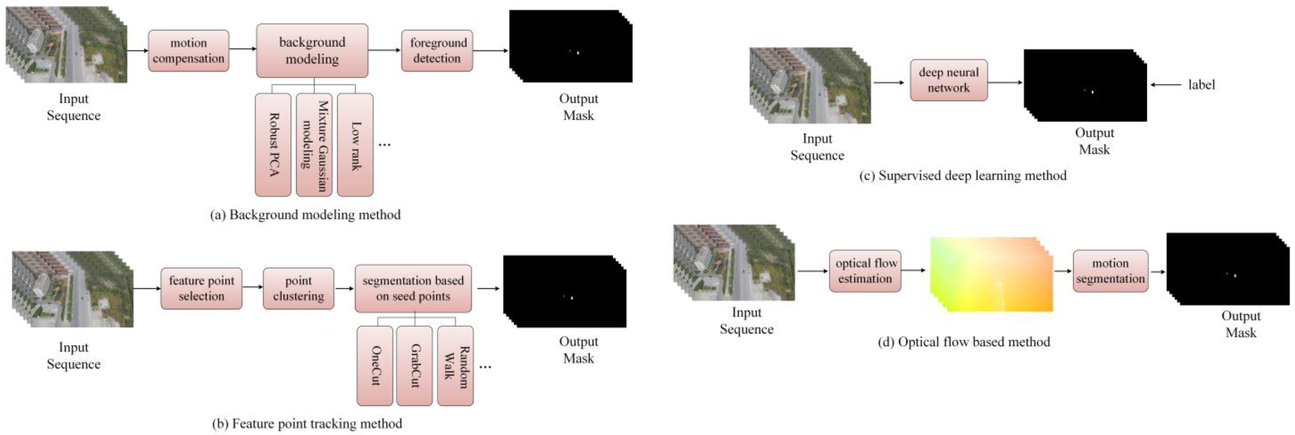
- Background modeling methods
- B.
- Feature point tracking methods
- C.
- Supervised deep learning methods
- D.
- Optical flow-based methods
2.2. Development of Optical Flow-Based Moving Object Detection Methods
2.3. Development of Moving Object Detection in UAV Scenarios
3. Approach
3.1. Framework
3.2. Loss Function
3.2.1. Flow Reconstruction Loss
3.2.2. Spatial Consistency Loss
3.2.3. Temporal Consistency Loss
3.2.4. Foreground Sparse Loss
4. Experiments
4.1. Datasets
4.2. Implementation Details
4.3. Evaluation Metrics
4.4. Quantitative Results
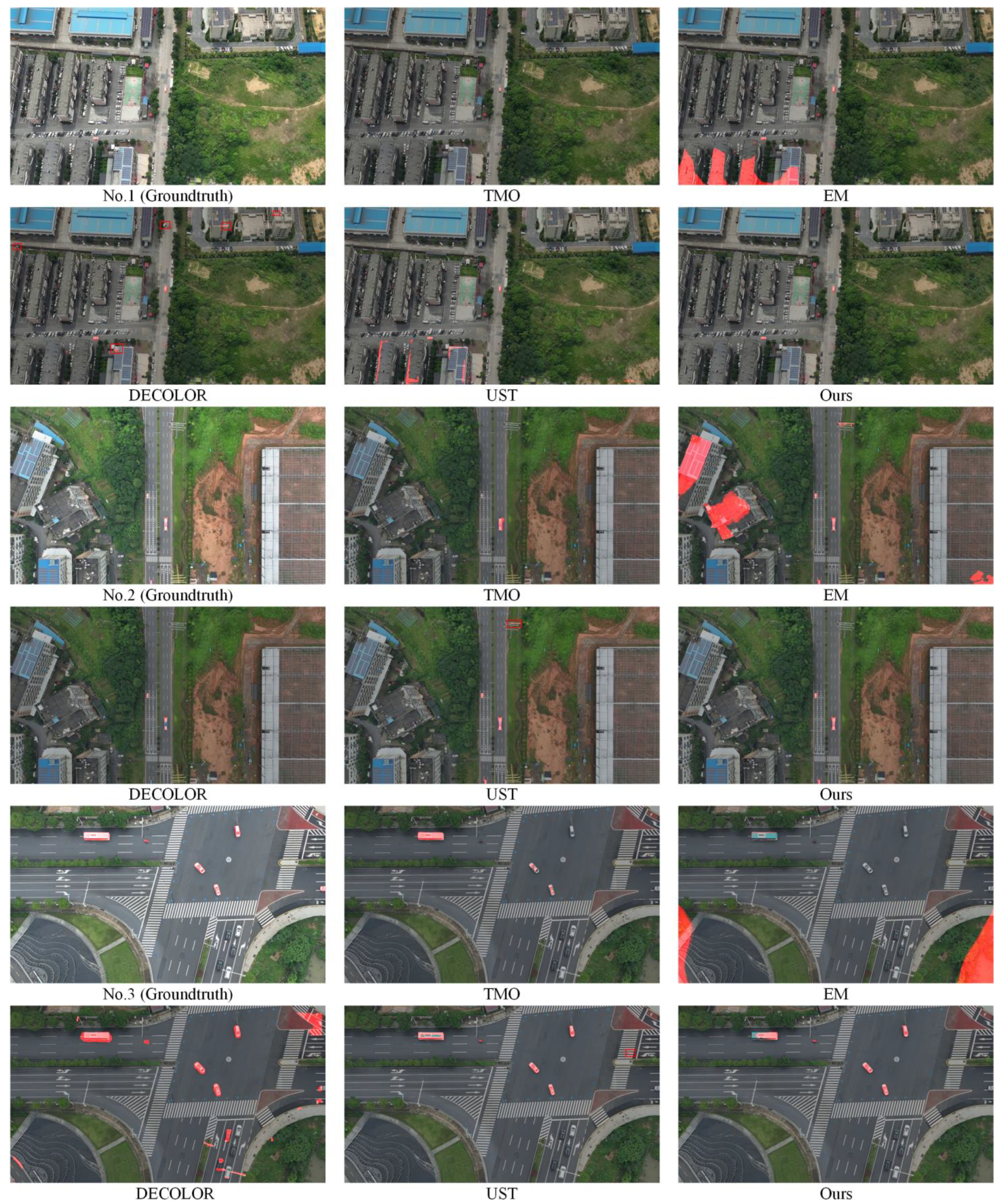
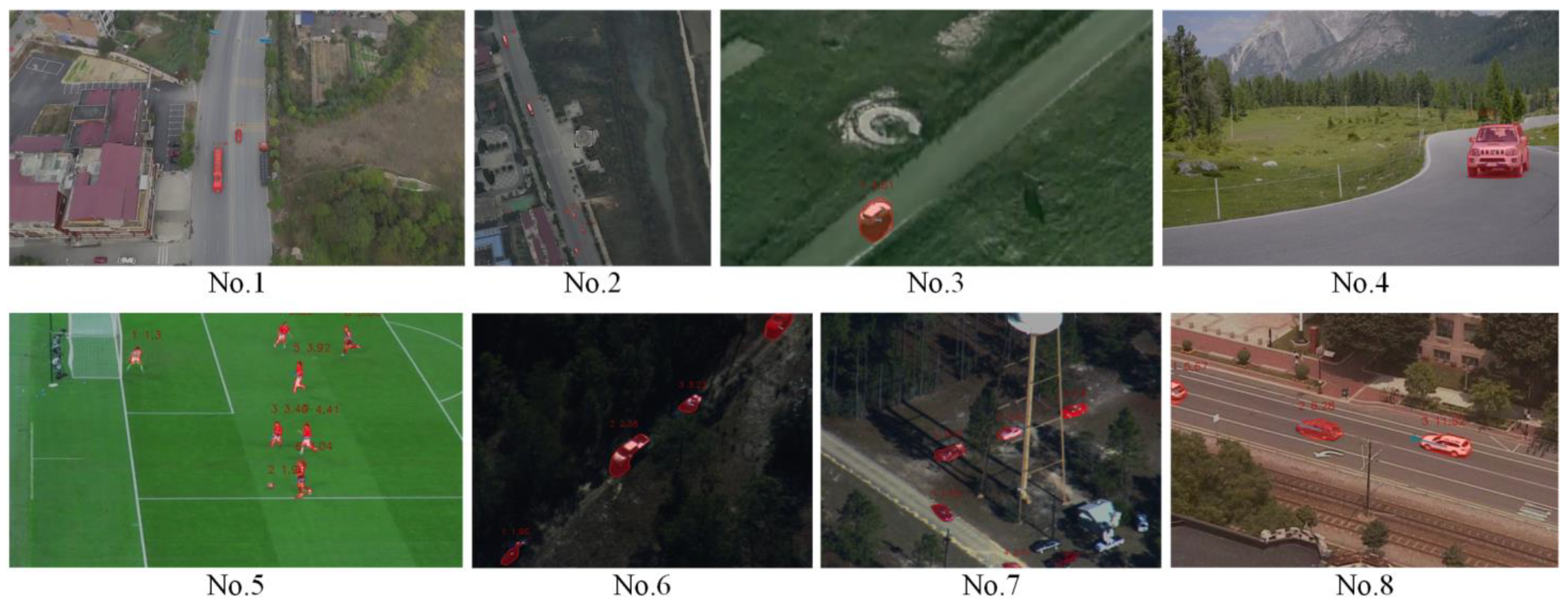
4.5. Qualitative Results
4.6. Ablation Results
4.7. Cross-Dataset Results
5. Conclusions
Author Contributions
Funding
Data Availability Statement
Conflicts of Interest
Appendix A
Appendix A.1. Pseudocode of the Proposed Method
| Algorithm A1 Proposed Moving Object Detection method | |
| 1: | procedure FlowPrepare) |
| 2: | |
| 3: | end procedure |
| 4: | procedure TrainingStep) |
| 5: | |
| 6: | |
| 7: | (Equation 3) |
| 8: | (Equations 4, 5 and 6) |
| 9: | |
| 10: | |
| 11: | end procedure |
| 12: | procedure InferenceStep) |
| 13: | |
| 14: | end procedure |
Appendix A.2. Example of Occlusion Scenarios
Appendix A.3. Example of Occlusion Scenarios
References
- Zhou, X.; Yang, C.; Yu, W. Moving Object Detection by Detecting Contiguous Outliers in the Low-Rank Representation. IEEE Trans. Pattern Anal. Mach. Intell. 2013, 35, 597–610. [Google Scholar] [CrossRef]
- Mandal, M.; Kumar, L.K.; Vipparthi, S.K. Mor-uav: A benchmark dataset and baselines for moving object recognition in uav videos. In Proceedings of the 28th ACM International Conference on Multimedia, Seattle, WA, USA, 12–16 October 2020. [Google Scholar]
- Koffka, K. Perception: An introduction to the Gestalt-theorie. Psychol. Bull. 1922, 19, 531–585. [Google Scholar] [CrossRef]
- Perazzi, F.; Pont-Tuset, J.; McWilliams, B.; Van Gool, L.; Gross, M.; Sorkine-Hornung, A.; Zurich, E.T.H. Disney Research. A benchmark dataset and evaluation methodology for video object segmentation. In Proceedings of the IEEE Conference on Computer Vision and Pattern Recognition, Las Vegas, NV, USA, 27–30 June 2016. [Google Scholar]
- Collins, R.; Zhou, X.; The, S.K. An open source tracking testbed and evaluation web site. In Proceedings of the IEEE International Workshop on Performance Evaluation of Tracking and Surveillance (PETS 2005), Breckenridge, CO, USA, 10 January 2005. [Google Scholar]
- Stauffer, C.; Grimson, W.E.L. Adaptive background mixture models for real-time tracking. In Proceedings of the IEEE Computer Society Conference on Computer Vision and Pattern Recognition, Fort Collins, CO, USA, 23–25 June 1999. [Google Scholar]
- Zivkovic, Z. Improved adaptive Gaussian mixture model for background subtraction. In Proceedings of the 17th International Conference on Pattern Recognition (ICPR 2004), Cambridge, UK, 23–26 August 2004. [Google Scholar]
- Lee, D.-S. Effective Gaussian mixture learning for video background subtraction. IEEE Trans. Pattern Anal. Mach. Intell. 2005, 27, 827–832. [Google Scholar]
- Shakeri, M.; Zhang, H. COROLA: A sequential solution to moving object detection using low-rank approximation. Comput. Vis. Image Underst. 2016, 146, 27–39. [Google Scholar] [CrossRef]
- ElTantawy, A.; Shehata, M.S. KRMARO: Aerial Detection of Small-Size Ground Moving Objects Using Kinematic Regularization and Matrix Rank Optimization. IEEE Trans. Circuits Syst. Video Technol. 2019, 29, 1672–1686. [Google Scholar] [CrossRef]
- Marc, V.D.; Barnich, O. ViBE: A Powerful Random Technique to Estimate the Background in Video Sequences. In Proceedings of the IEEE International Conference on Acoustics, Speech and Signal Processing, Taipei, Taiwan, 19–24 April 2009. [Google Scholar]
- Sheikh, Y.; Javed, O.; Kanade, T. Background Subtraction for Freely Moving Cameras. In Proceedings of the IEEE International Conference on Computer Vision, Kyoto, Japan, 29 September–2 October 2009. [Google Scholar]
- Berger, M.; Seversky, L. Subspace Tracking under Dynamic Dimensionality for Online Background Subtraction. In Proceedings of the IEEE Conference on Computer Vision and Pattern Recognition, Columbus, OH, USA, 23–28 June 2014. [Google Scholar]
- Wang, Y.; Yu, Z.; Zhu, L. Foreground Detection with Deeply Learned Multi-Scale Spatial-Temporal Features. Sensors 2018, 18, 4269. [Google Scholar] [CrossRef]
- Lim, K.; Jang, W.-D.; Kim, C.-S. Background Subtraction Using Encoder-Decoder Structured Convolutional Neural Network. In Proceedings of the 14th IEEE International Conference on Advanced Video and Signal Based Surveillance (AVSS), Lecce, Italy, 29 August–1 September 2017. [Google Scholar]
- Lim, L.A.; Keles, H.Y. Learning Multi-scale Features for Foreground Segmentation. Pattern Anal. Appl. 2018, 23, 1369–1380. [Google Scholar] [CrossRef]
- Teed, Z.; Deng, J. Raft: Recurrent All-Pairs Field Transforms for Optical Flow. In Proceedings of the European Conference on Computer Vision, Glasgow, UK, 23–28 August 2020. [Google Scholar]
- Huang, Z.; Shi, X.; Zhang, C.; Wang, Q.; Cheung, K.C.; Qin, H.; Dai, J.; Li, H. Flowformer: A Transformer Architecture for Optical Flow. In Proceedings of the European Conference on Computer Vision, Tel Aviv, Israel, 23–27 October 2022. [Google Scholar]
- Kim, J.; Wang, X.; Wang, H.; Zhu, C.; Kim, D. Fast Moving Object Detection with Non-Stationary Background. Multimed. Tools Appl. 2012, 67, 311–335. [Google Scholar] [CrossRef]
- Bugeau, A.; Pérez, P. Detection and segmentation of moving objects in complex scenes. Comput. Vis. Image Underst. 2009, 113, 459–476. [Google Scholar] [CrossRef]
- Brox, T.; Malik, J. Object Segmentation by Long Term Analysis of Point Trajectories. In Proceedings of the European Conference on Computer Vision, Heraklion, Crete, Greece, 5–11 September 2010. [Google Scholar]
- Huang, J.; Zou, W.; Zhu, J.; Zhu, Z. Optical Flow Based Real-time Moving Object Detection in Unconstrained Scenes. arXiv 2018, arXiv:1807.04890. [Google Scholar]
- Sugimura, D.; Teshima, F.; Hamamoto, T. Online background subtraction with freely moving cameras using different motion boundaries. Image Vis. Comput. 2018, 76, 76–92. [Google Scholar] [CrossRef]
- Zhang, W.; Sun, X.; Yu, Q. Moving Object Detection under a Moving Camera via Background Orientation Reconstruction. Sensors 2020, 20, 3103. [Google Scholar] [CrossRef]
- Zhang, W.; Sun, X.; Yu, Q. Accurate moving object segmentation in unconstraint videos based on robust seed pixels selection. Int. J. Adv. Robot. Syst. 2020, 17, 1–11. [Google Scholar] [CrossRef]
- Tokmakov, P.; Alahari, K.; Schmid, C. Learning motion patterns in videos. In Proceedings of the IEEE Conference on Computer Vision and Pattern Recognition (CVPR), Honolulu, HI, USA, 21–26 July 2017. [Google Scholar]
- Yang, C.; Lamdouar, H.; Lu, E.; Zisserman, A.; Xie, W. Self supervised video object segmentation by motion grouping. In Proceedings of the International Conference on Computer Vision (ICCV), Montreal, QC, Canada, 11–17 October 2021. [Google Scholar]
- Yang, Y.; Lai, B.; Soatto, S. DyStaB: Unsupervised object segmentation via dynamic-static bootstrapping. In Proceedings of the IEEE Conference on Computer Vision and Pattern Recognition (CVPR), Nashville, TN, USA, 20–25 June 2021. [Google Scholar]
- Zhou, T.; Li, J.; Wang, S.; Tao, R.; Shen, J. MATNet: Motion-Attentive Transition Network for Zero-Shot Video Object Segmentation. IEEE Trans. Image Process. 2020, 29, 8326–8338. [Google Scholar] [CrossRef] [PubMed]
- Ge, P.; Fu, K.; Wu, Z.; Fan, D.P.; Shen, J.; Shao, L. Full-Duplex Strategy for Video Object Segmentation. In Proceedings of the IEEE/CVF International Conference on Computer Vision (ICCV), Montreal, QC, Canada, 11–17 October 2021. [Google Scholar]
- Shu, Y.; Zhang, L.; Qi, J.; Lu, H.; Wang, S.; Zhang, X. Learning Motion-Appearance Co-Attention for Zero-Shot Video Object Segmentation. In Proceedings of the IEEE/CVF International Conference on Computer Vision (ICCV), Montreal, QC, Canada, 11–17 October 2021. [Google Scholar]
- Choudhury, S.; Karazija, L.; Laina, I.; Vedaldi, A.; Rupprecht, C. Guess What Moves: Unsupervised Video and Image Segmentation by Anticipating Motion. In Proceedings of the British Machine Vision Conference (BMVC), London, UK, 2022., 21–24 November.
- Meunier, E.; Badoual, A.; Bouthemy, P. EM-Driven Unsupervised Learning for Efficient Motion Segmentation. IEEE Trans. Pattern Anal. Mach. Intell. 2023, 45, 4462–4473. [Google Scholar] [CrossRef]
- Meunier, E.; Bouthemy, P. Unsupervised Space-Time Network for Temporally-Consistent Segmentation of Multiple Motions. In Proceedings of the IEEE/CVF Conference on Computer Vision and Pattern Recognition (CVPR), Vancouver, BC, Canada, 17–24 June 2023. [Google Scholar]
- Suhwan, C.; Lee, M.; Lee, S.; Park, C.; Kim, D.; Lee, S. Treating Motion as Option to Reduce Motion Dependency in Unsupervised Video Object Segmentation. In Proceedings of the 2023 IEEE/CVF Winter Conference on Applications of Computer Vision (WACV), Waikoloa, HI, USA, 2–7 January 2023. [Google Scholar]
- Logoglu, K.B.; Lezki, H.; Yucel, M.K.; Ozturk, A.; Kucukkomurler, A.; Karagoz, B.; Erdem, E.; Erdem, A. Feature-Based Efficient Moving Object Detection for Low-Altitude Aerial Platforms. In Proceedings of the IEEE International Conference on Computer Vision Workshops (ICCVW), Venice, Italy, 22–29 October 2017. [Google Scholar]
- Mueller, M.; Smith, N.; Ghanem, B. A Benchmark and Simulator for UAV Tracking. In Proceedings of the European Conference on Computer Vision (ECCV), Amsterdam, The Netherlands, 11–14 October 2016. [Google Scholar]
- Lezki, H.; Ozturk, I.A.; Akpinar, M.A.; Yucel, M.K.; Logoglu, K.B.; Erdem, A.; Erdem, E. Joint Exploitation of Features and Optical Flow for Real-Time Moving Object Detection on Drones. In Proceedings of the European Conference on Computer Vision (ECCV) Workshops, Munich, Germany, 8–14 September 2018. [Google Scholar]
- Kalantar, B.; Mansor, S.B.; Halin, A.A.; Shafri, H.Z.M.; Zand, M. Multiple Moving Object Detection From UAV Videos Using Trajectories of Matched Regional Adjacency Graphs. IEEE Trans. Geosci. Remote Sens. 2017, 55, 5198–5213. [Google Scholar] [CrossRef]
- Siam, M.; Eikerdawy, S.; Gamal, M.; Abdel-Razek, M.; Jagersand, M.; Zhang, H. Real-Time Segmentation with Appearance, Motion and Geometry. In Proceedings of the 2018 IEEE/RSJ International Conference on Intelligent Robots and Systems (IROS), Madrid, Spain, 1–5 October 2018. [Google Scholar]
- Li, J.; Ye, D.H.; Kolsch, M.; Wachs, J.P.; Bouman, C.A. Fast and Robust UAV to UAV Detection and Tracking From Video. IEEE Trans. Emerg. Top. Comput. 2022, 10, 1519–1531. [Google Scholar] [CrossRef]
- Kimura, M.; Shibasaki, R.; Shao, X.; Nagai, M. Automatic Extraction of Moving Objects from UAV-Borne Monocular Images Using Multi-View Geometric Constraints. In Proceedings of the International Micro Air Vehicle Conference and Competition (IMAV 2014), Delft, The Netherlands, 12–15 August 2014. [Google Scholar]
- Çiçek, Ö.; Abdulkadir, A.; Lienkamp, S.S.; Brox, T.; Ronneberger, O. 3D U-Net: Learning Dense Volumetric Segmentation from Sparse Annotation. In Proceedings of the Medical Image Computing and Computer-Assisted Intervention, Athens, Greece, 17–21 October 2016. [Google Scholar]
- Liu, D.; Nocedal, J. On the Limited Memory BFGS Method for Large Scale Optimization. Math. Program. 1989, 45, 503–528. [Google Scholar] [CrossRef]
- Horn, B.; Schunck, B. Determining Optical Flow. Artif. Intell. 1981, 16, 185–203. [Google Scholar] [CrossRef]
- Li, S.Z. Markov Random Field Modeling in Image Analysis; Springer: Tokyo, Japan, 2009. [Google Scholar]
- Kingma, D.P.; Ba, J. Adam: A Method for Stochastic Optimization. arXiv 2014, arXiv:1412.6980. [Google Scholar]
- Wu, Y.; He, X.; Nguyen, T.Q. Moving Object Detection with a Freely Moving Camera via Background Motion Subtraction. IEEE Trans. Circuits Syst. Video Technol. 2017, 27, 236–248. [Google Scholar] [CrossRef]
- Wu, S.; Oreifej, O.; Shah, M. Action Recognition in Videos Acquired by a Moving Camera Using Motion Decomposition of Lagrangian Particle Trajectories. In Proceedings of the IEEE International Conference on Computer Vision (ICCV), Barcelona, Spain, 6–13 November 2011. [Google Scholar]
- Hartley, R.; Zisserman, A. Multiple View Geometry in Computer Vision, 2nd ed.; Cambridge University Press: Cambridge, UK, 2004; pp. 123–126. [Google Scholar]
- Wang, Y.; Jodoin, P.M.; Porikli, F.; Konrad, J.; Benezeth, Y.; Ishwar, P. CDnet 2014: An Expanded Change Detection Benchmark Dataset. In Proceedings of the IEEE Conference on Computer Vision and Pattern Recognition Workshops, Columbus, OH, USA, 23–28 June 2014. [Google Scholar]


| Method | JI (%) | Pr (%) | Re (%) | F1 (%) |
|---|---|---|---|---|
| TMO [35] | 21.01 | 21.16 | 19.87 | 20.49 |
| EM [33] | 20.83 | 35.02 | 59.40 | 44.06 |
| DECOLOR [1] | 45.85 | 44.36 | 68.58 | 53.88 |
| UST [34] | 39.07 | 53.94 | 61.33 | 57.40 |
| Ours | 53.01 | 61.85 | 63.44 | 62.64 |
| Data | TMO [35] | BMS [48] | MD [49] | HOMO [50] | EM [33] | UST [34] | Ours |
|---|---|---|---|---|---|---|---|
| Car4 | 0.92 | 0.87 | 0.67 | 0.78 | 0.91 | 0.81 | 0.87 |
| Car5 | 0.88 | 0.84 | 0.55 | 0.80 | 0.90 | 0.82 | 0.88 |
| Car6 | 0.93 | 0.91 | 0.44 | 0.86 | 0.92 | 0.92 | 0.92 |
| Car7 | 0.90 | 0.91 | 0.75 | 0.89 | 0.89 | 0.83 | 0.88 |
| Seq. 1 | 0.53 | 0.83 | 0.58 | 0.66 | 0.70 | 0.73 | 0.71 |
| Seq. 2 | 0.78 | 0.85 | 0.74 | 0.69 | 0.77 | 0.75 | 0.75 |
| Seq. 5 | 0.67 | 0.63 | 0.40 | 0.46 | 0.30 | 0.49 | 0.60 |
| Seq. 6 | 0.77 | 0.60 | 0.28 | 0.49 | 0.75 | 0.60 | 0.68 |
| Seq. 7 | 0.93 | 0.90 | 0.19 | 0.85 | 0.93 | 0.92 | 0.93 |
| Average | 0.82 | 0.82 | 0.51 | 0.72 | 0.80 | 0.77 | 0.81 |
| Method | JI (%) | Pr (%) | Re (%) | F1 (%) |
|---|---|---|---|---|
| Baseline | 39.07 | 53.94 | 61.33 | 57.40 |
| Base + sb | 50.09 | 58.92 | 62.46 | 60.64 |
| Base + sb + sp | 51.70 | 61.41 | 61.10 | 61.26 |
| Ours | 53.01 | 61.85 | 63.44 | 62.64 |
Disclaimer/Publisher’s Note: The statements, opinions and data contained in all publications are solely those of the individual author(s) and contributor(s) and not of MDPI and/or the editor(s). MDPI and/or the editor(s) disclaim responsibility for any injury to people or property resulting from any ideas, methods, instructions or products referred to in the content. |
© 2025 by the authors. Licensee MDPI, Basel, Switzerland. This article is an open access article distributed under the terms and conditions of the Creative Commons Attribution (CC BY) license (https://creativecommons.org/licenses/by/4.0/).
Share and Cite
Fan, X.; Wen, G.; Gao, Z.; Chen, J.; Jian, H. An Unsupervised Moving Object Detection Network for UAV Videos. Drones 2025, 9, 150. https://doi.org/10.3390/drones9020150
Fan X, Wen G, Gao Z, Chen J, Jian H. An Unsupervised Moving Object Detection Network for UAV Videos. Drones. 2025; 9(2):150. https://doi.org/10.3390/drones9020150
Chicago/Turabian StyleFan, Xuxiang, Gongjian Wen, Zhinan Gao, Junlong Chen, and Haojun Jian. 2025. "An Unsupervised Moving Object Detection Network for UAV Videos" Drones 9, no. 2: 150. https://doi.org/10.3390/drones9020150
APA StyleFan, X., Wen, G., Gao, Z., Chen, J., & Jian, H. (2025). An Unsupervised Moving Object Detection Network for UAV Videos. Drones, 9(2), 150. https://doi.org/10.3390/drones9020150