


A Bound-Preserving Numerical Scheme for Space–Time Fractional Advection Equations

Abstract
1. Introduction
2. Derivation of Explicit Numerical Schemes
2.1. An Explicit Numerical Scheme for sFAE (3)
2.2. An Explicit Numerical Scheme for stFAE (1)
2.3. Stability and Error Analysis of the EFDM for sFDE
2.4. A Fast Implementation
3. A Finite Difference Approximation for stFDE (1)
3.1. Error Analysis and Stability of the EFDM for stFDE
3.2. A Fast-Evaluation-in-Time Implementation
4. Numerical Experiments
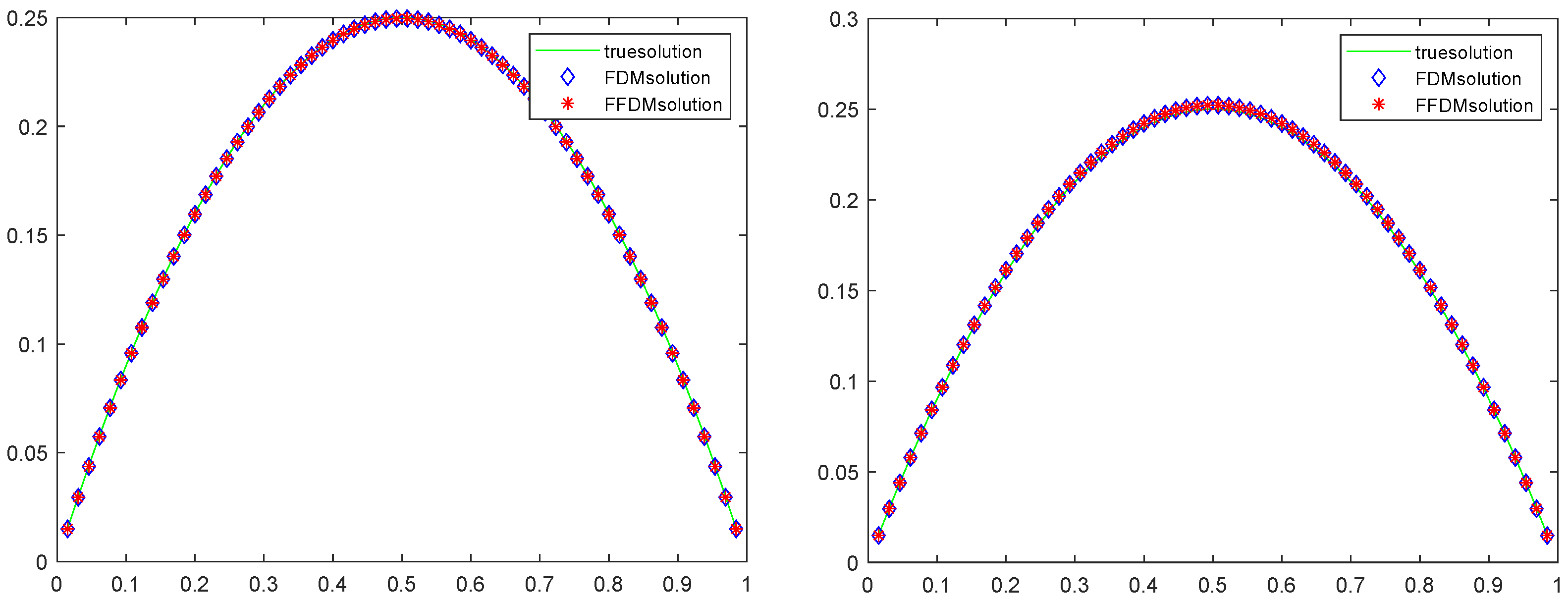
4.1. The Convergence and Performance of Both Methods
- (i)
- FFDM can effectively reduce the costs of computation and memory requirement, which is to say that FFDM has a much better efficiency than FDM.
- (ii)
- (iii)
- In Table 4, one can see that we only show the two cases where and because the result is unsteady when is for as they did not satisfy the CFL condition, which strongly confirm the theories.
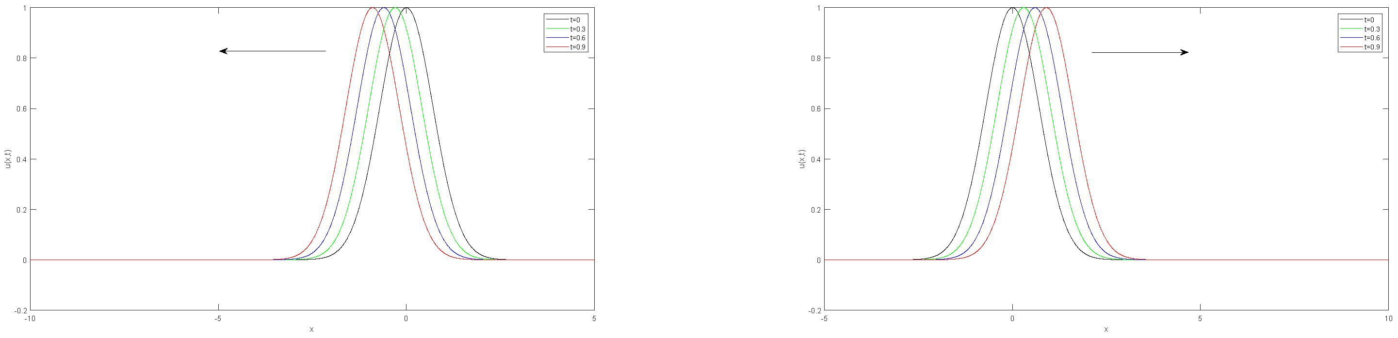
4.2. Anomalous Diffusive Transport
5. Discussion and Conclusions
Author Contributions
Funding
Data Availability Statement
Acknowledgments
Conflicts of Interest
References
- Metzler, R.; Klafter, J. The restaurant at the end of the random walk: Recent developments in the description of anomalous transport by fractional dynamics. J. Phys. A Math. Gen. 2004, 37, R161–R208. [Google Scholar] [CrossRef]
- Podlubny, I. Fractional Differential Equations; Academic Press: Cambridge, MA, USA, 1999. [Google Scholar]
- Diethelm, K.; Ford, N. A note on the well-posedness of terminal value problems for fractional differential equations. J. Integral Equ. Appl. 2017, 30, 371–376. [Google Scholar] [CrossRef]
- Zhang, X.; Yu, L.; Jiang, J.; Wu, Y.; Cui, Y. Positive Solutions for a Weakly Singular Hadamard-Type Fractional Differential Equation with Changing-Sign Nonlnearity. J. Funct. Spaces 2020, 2020, 5623589. [Google Scholar]
- Zhang, X.; Yu, L.; Jiang, J.; Wu, Y.; Cui, Y. Solutions for a Singular Hadamard-Type Fractional Differential Equation by the Spectral Construct Analysis. J. Funct. Spaces 2020, 2020, 8392397. [Google Scholar] [CrossRef]
- He, J.; Zhang, X.; Liu, L.; Wu, Y.; Cui, Y. A singular fractional Kelvin-Voigt model involving a nonlinear operator and their convergence properties. Bound. Value Probl. 2019, 2019, 112. [Google Scholar] [CrossRef]
- Wu, J.; Zhang, X.; Liu, L.; Wu, Y.; Cui, Y. The convergence analysis and error estimation for unique solution of a p-Laplacian fractional differential equaion with singular decreasing nonlinearity. Bound. Value Probl. 2018, 2018, 82. [Google Scholar] [CrossRef]
- Chen, H.; Wang, H. Numerical simulation for conservative fractional diffusion equations by an expanded mixed formulation. J. Comput. Appl. Math. 2016, 296, 480–498. [Google Scholar] [CrossRef]
- Ervin, V.; Heuer, N.; Roop, J. Regularity of the solution to 1-D fractional order diffusion equations. Math. Comput. 2018, 87, 2273–2294. [Google Scholar] [CrossRef]
- Zheng, X.; Wang, H. An error estimate of a numerical approximation to a hidden-memory variable-order space-time fractional diffusion equation. SIAM J. Numer. Anal. 2020, 58, 2492–2514. [Google Scholar] [CrossRef]
- Zheng, X.; Wang, H. An optimal-order numerical approximation to variable-order space-fractional diffusion equations on uniform or graded meshes. SIAM J. Numer. Anal. 2020, 58, 330–352. [Google Scholar] [CrossRef]
- Deng, W.; Li, C.; Lü, J. Stability analysis of linear fractional differential system with multiple time delays. Nonlinear Dyn. 2007, 48, 409–416. [Google Scholar] [CrossRef]
- Zheng, X.; Wang, H. A hidden-memory variable-order fractional optimal control model: Analysis and approximation. SIAM J. Control Optim. 2021, 59, 1851–1880. [Google Scholar] [CrossRef]
- Yu, B.; Zheng, X.; Zhang, P.; Zhang, L. Computing solution landscape of nonlinear space-fractional problems via fast approximation algorithm. J. Comput. Phys. 2022, 468, 111513. [Google Scholar] [CrossRef]
- Gu, X.; Huang, T.; Ji, C.; Carpentieri, B.; Alikhanov, A.A. Fast iterative method with a second-order implicit difference scheme for time-space fractional convection-diffusion equation. J. Sci. Comput. 2017, 72, 957–985. [Google Scholar] [CrossRef]
- Ren, T.; Li, S.; Zhang, X.; Liu, L. Maximum and minimum solutions for a nonlocal p-Laplacian fractional differential system from eco-economical processes. Bound. Value Probl. 2017, 2017, 118. [Google Scholar] [CrossRef]
- Wu, J.; Zhang, X.; Liu, L.; Wu, Y.; Cui, Y. Convergence analysis of iterative scheme and error estimation of positive solution for a fractional differential equation. Math. Model. Anal. 2018, 23, 611–626. [Google Scholar]
- Garrappa, R.; Moret, I.; Popolizio, M. Solving the time-fractional Schrödinger equation by Krylov projection methods. J. Comput. Phys. 2015, 293, 115–134. [Google Scholar] [CrossRef]
- Jia, L.; Chen, H.; Wang, H. Mixed-type Galerkin variational principle and numerical simulation for a generalized nonlocal elastic model. J. Sci. Comput. 2017, 71, 660–681. [Google Scholar] [CrossRef]
- Liu, F.; Anh, V.; Turner, I. Numerical solution of the space fractional Fokker-Planck equation. J. Comput. Appl. Math 2004, 166, 209–219. [Google Scholar] [CrossRef]
- Jin, B.; Li, B.; Zhou, Z. Discrete maximal regularity of time-stepping schemes for fractional evolution equations. Numer. Math. 2018, 138, 101–131. [Google Scholar] [CrossRef]
- Wang, H.; Yang, D. Wellposedness of variable-coefficient conservative fractional elliptic differential equations. SIAM Numer. Anal. 2013, 51, 1088–1107. [Google Scholar] [CrossRef]
- Gao, J.; Zhao, M.; Du, N.; Guo, X.; Wang, H.; Zhang, J. A finite element method for space-time directional fractional diffusion partial differential equations in the plane and its error analysis. J. Comput. Appl. Math. 2019, 362, 354–365. [Google Scholar] [CrossRef]
- Meerschaert, M.M.; Tadjeran, C. Finite difference approximations for two-sided space-fractional partial differential equations. Appl. Numer. Math. 2006, 56, 80–90. [Google Scholar] [CrossRef]
- Roos, H.G.; Stynes, M.; Tobiska, L. Robust Numerical Methods for Singularly Perturbed Differential Equations; Springer: Berlin/Heidelberg, Germany, 2008. [Google Scholar]
- Zhang, X.; Shu, C. On maximum-principle-satisfying high order schemes for scalar conservation laws. J. Comput. Phys. 2010, 229, 3091–3120. [Google Scholar] [CrossRef]
- Zhang, X.; Shu, C. Maximum-principle-satisfying and positivity-preserving high order schemes for conservation laws: Survey and new developments. Proc. R. Soc. A 2011, 467, 2752–2776. [Google Scholar] [CrossRef]
- Zhang, X.; Shu, C. Positivity-preserving high order discontinuous Galerkin schemes for compressible Euler equations with source terms. J. Comput. Phys. 2011, 230, 1238–1248. [Google Scholar] [CrossRef]
- Du, J.; Yang, Y. High-order bound-preserving discontinuous Galerkin methods for multicomponent chemically reacting flows. J. Comput. Phys. 2022, 469, 111548. [Google Scholar] [CrossRef]
- Zhang, Y.; Zhang, X.; Shu, C. Maximum-principle-satisfying second order discontinuous Galerkin schemes for convection-diffusion equations on triangular meshes. J. Comput. Phys. 2003, 234, 295–316. [Google Scholar] [CrossRef]
- Jia, J.; Wang, H. A fast finite volume method for conservative space-time fractional diffusion equations discretized on space-time locally refined meshes. Comput. Math. Appl. 2019, 78, 1345–1356. [Google Scholar] [CrossRef]
- Jia, J.; Wang, H. A fast finite volume method on locally refined meshes for fractional diffusion equations. East Asian J. Appl. Math. 2019, 9, 755–779. [Google Scholar]
- Wang, H.; Basu, T.S. A fast finite difference method for two-dimensional space-fractional diffusion equations. SIAM Sci. Comput. 2012, 34, A2444–A2458. [Google Scholar] [CrossRef]
- Du, N.; Wang, H. A Fast Finite Element Method for Space-Fractional Dispersion Equations on Bounded Domains in R2. SIAM J. Sci. Comput. 2015, 37, A1614–A1635. [Google Scholar] [CrossRef]
- Wang, H.; Wang, K.; Sircar, T. A direct O(Nlog2N) finite difference method for fractional diffusion equations. J. Comput. Phys. 2010, 229, 8095–8104. [Google Scholar] [CrossRef]
- Lin, Y.; Xu, C. Finite difference/spectral approximation for the time-fractional diffusion equation. J. Comput. Phys. 2007, 225, 1533–1552. [Google Scholar] [CrossRef]
- De Moura, C.A.; Kubrusly, C.S. The Courant-Friedrichs-Lewy Condition; AMC: Leawood, UK, 2013. [Google Scholar]
- Chan, R.H.; Ng, M.K. Conjugate gradient methods for Toeplitz systems. SIAM Rev. 1996, 38, 427–482. [Google Scholar] [CrossRef]
- Davis, P.J. Circulant Matrices; American Mathematical Society: Providence, RI, USA, 2012. [Google Scholar]
- Jiang, S.; Zhang, J.; Zhang, Q.; Zhang, Z. Fast evaluation of the Caputo fractional derivative and its applications to fractional diffusion equations. arXiv 2015, arXiv:1511.03453. [Google Scholar] [CrossRef]
- Xu, Q.; Hesthaven, J.S. Discontinuous Galerkin Method For Fractional Convection-Diffusion Equations. SIAM J. Numer. Anal. 2014, 52, 405–423. [Google Scholar] [CrossRef]
- Baccouch, M.; Temimi, H. Analysis of Optimal Error Estimates and Superconvergence of the Discontinuous Galerkin Method for Convection-Diffusion Problems in one Space Dimension. Int. J. Numer. Anal. Model. 2016, 13, 403–434. [Google Scholar]
- Deng, W.; Hesthaven, J.S. Local discontinuous Galerkin methods for fractional diffusion equations. ESAIM Math. Modell. Numer. Anal. 2013, 47, 1845–1864. [Google Scholar] [CrossRef]
- Ren, J.; Sun, Z.; Zhao, X. Compact difference scheme for the fractional sub-diffusion equation with Neumann boundary conditions. J. Comput. Phys. 2012, 232, 456–467. [Google Scholar] [CrossRef]
- Zhang, Y.; Sun, Z.; Zhao, X. Compact alternating direction implicit scheme for the two-dimensional fractional diffusion-wave equation. SIAM J. Numer. Anal. 2012, 50, 1535–1555. [Google Scholar] [CrossRef]


| M | FDM | FFDM | ||||
|---|---|---|---|---|---|---|
| Error | CPU Time | Error | CPU Time | |||
| 0.0021 | - | 14.25 s | 0.0021 | - | 8.78 s | |
| 0.0010 | 1.0704 | 3 min 52 s | 0.0010 | 1.0704 | 17.05 s | |
| 5.2135 | 0.9397 | 10 min 27 s | 5.2135 | 0.9397 | 33.63 s | |
| - | - | Out of memory | 2.6067 | 1.0000 | 66.67 s | |
| - | - | Out of memory | 1.3033 | 1.0001 | 2 min 14 s | |
| FDM | FFDM | ||||
|---|---|---|---|---|---|
| -Error | -Error | ||||
| 2.3313 | - | 2.3313 | - | ||
| 7.9127 | 1.5589 | 7.9127 | 1.5589 | ||
| 2.0332 | 1.9604 | 2.0332 | 1.9604 | ||
| 3.1985 | 2.6683 | 3.1985 | 2.6683 | ||
| 6.6565 | - | 6.6565 | - | ||
| 2.6633 | 1.3215 | 2.6633 | 1.3215 | ||
| 9.5791 | 1.4753 | 9.5791 | 1.4753 | ||
| 2.8968 | 1.7254 | 2.8968 | 1.7254 | ||
| 4.9270 | 2.5557 | 4.9270 | 2.5557 | ||
| 0.0016 | - | 0.0016 | - | ||
| 7.3537 | 1.1215 | 7.3537 | 1.1215 | ||
| 3.1433 | 1.2262 | 3.1433 | 1.2262 | ||
| 1.2657 | 1.3123 | 1.2657 | 1.3123 | ||
| 4.6550 | 1.4431 | 4.6550 | 1.4431 | ||
| M | FDM | FFDM | ||||
|---|---|---|---|---|---|---|
| Error | Rate | CPU Time | Error | Rate | CPU Time | |
| 0.0013 | - | 1.43 s | 0.0013 | - | 1.35 s | |
| 6.7777 | 0.9392 | 15.0 s | 6.7777 | 0.9392 | 10.6 s | |
| 3.4326 | 0.9820 | 4 min 38 s | 3.4326 | 0.9820 | 1 min 53 s | |
| - | - | Out of memory | 1.7335 | 0.9856 | 10 min 56 s | |
| - | - | Out of memory | 8.7323 | 0.9893 | 1 h 33 min 49 s | |
| - | - | Out of memory | 4.3901 | 0.9921 | 12 h 51 min 6 s | |
| M | FDM | FFDM | |||
|---|---|---|---|---|---|
| Error | Error | ||||
| 0.3 | 2.7251 | - | 2.7251 | - | |
| 9.1584 | 1.5669 | 9.1584 | 1.5669 | ||
| 3.0983 | 1.5699 | 3.0983 | 1.5699 | ||
| 1.0531 | 1.5568 | 1.0531 | 1.5568 | ||
| 3.6480 | 1.5295 | 3.6480 | 1.5295 | ||
| 0.5 | 6.9408 | - | 6.9408 | - | |
| 2.5789 | 1.4283 | 2.5789 | 1.4283 | ||
| 9.4645 | 1.4462 | 9.4645 | 1.4462 | ||
| 3.4528 | 1.4548 | 3.4528 | 1.4548 | ||
| 1.2575 | 1.4572 | 1.2575 | 1.4572 | ||
| 0.7 | 0.0015 | - | 0.00154 | - | |
| 6.3110 | 1.2490 | 6.3110 | 1.2490 | ||
| 2.6111 | 1.2732 | 2.6111 | 1.2732 | ||
| 1.0735 | 1.2823 | 1.0735 | 1.2823 | ||
| 4.3973 | 1.2876 | 4.3973 | 1.2876 | ||
| FDM | FFDM | ||||
|---|---|---|---|---|---|
| -Error | -Error | ||||
| 3.4169 | - | 3.4169 | - | ||
| 1.2196 | 1.4863 | 1.2196 | 1.4863 | ||
| 3.7410 | 1.7049 | 3.7410 | 1.7049 | ||
| 7.9030 | 2.2430 | 7.9030 | 2.2430 | ||
| 9.6137 | - | 9.6137 | - | ||
| 3.9324 | 1.2897 | 3.9324 | 1.2897 | ||
| 1.4755 | 1.4142 | 1.4755 | 1.4142 | ||
| 5.0551 | 1.5454 | 5.0551 | 1.5454 | ||
| 0.0023 | - | 0.0023 | - | ||
| 0.0011 | 1.0641 | 0.0011 | 1.0641 | ||
| 4.7942 | 1.1981 | 4.7942 | 1.1981 | ||
| 1.9961 | 1.2641 | 1.9961 | 1.2641 | ||
| M | FDM | FFDM | |||||
|---|---|---|---|---|---|---|---|
| Error | Rate | CPU Time | Error | Rate | CPU Time | ||
| 0.5 | 8.2859 | - | 1.80 s | 8.2859 | - | 1.88 s | |
| 4.2568 | 0.9598 | 15.3 s | 4.2568 | 0.9598 | 12.3 s | ||
| 2.1763 | 0.9690 | 3 min 59 s | 2.1763 | 0.9690 | 1 min 39 s | ||
| 1.1066 | 0.9757 | 6 h 37 min 7 s | 1.1066 | 0.9757 | 12 min 43 s | ||
| - | - | Out of memory | 5.6020 | 0.9821 | 1 h 42 min 2 s | ||
| - | - | Out of memory | 2.8261 | 0.9871 | 14 h 45 min 9 s | ||
| 0.7 | 8.8750 | - | 1.56 s | 8.8750 | - | 1.47 s | |
| 4.4614 | 0.9923 | 15.9 s | 4.4614 | 0.9923 | 12.3 s | ||
| 2.2392 | 0.9945 | 3 min 59 s | 2.2392 | 0.9945 | 1 m 39 s | ||
| 1.1212 | 0.9979 | 6 h 34 min 35 s | 1.1212 | 0.9979 | 12 min 39 s | ||
| - | - | Out of memory | 5.6031 | 1.0007 | 1 h 45 min 6 s | ||
| - | - | Out of memory | 2.7954 | 1.0032 | 15 h 38 min 33 s | ||
Disclaimer/Publisher’s Note: The statements, opinions and data contained in all publications are solely those of the individual author(s) and contributor(s) and not of MDPI and/or the editor(s). MDPI and/or the editor(s) disclaim responsibility for any injury to people or property resulting from any ideas, methods, instructions or products referred to in the content. |
© 2024 by the authors. Licensee MDPI, Basel, Switzerland. This article is an open access article distributed under the terms and conditions of the Creative Commons Attribution (CC BY) license (https://creativecommons.org/licenses/by/4.0/).
Share and Cite
Gao, J.; Chen, H. A Bound-Preserving Numerical Scheme for Space–Time Fractional Advection Equations. Fractal Fract. 2024, 8, 89. https://doi.org/10.3390/fractalfract8020089
Gao J, Chen H. A Bound-Preserving Numerical Scheme for Space–Time Fractional Advection Equations. Fractal and Fractional. 2024; 8(2):89. https://doi.org/10.3390/fractalfract8020089
Chicago/Turabian StyleGao, Jing, and Huaiguang Chen. 2024. "A Bound-Preserving Numerical Scheme for Space–Time Fractional Advection Equations" Fractal and Fractional 8, no. 2: 89. https://doi.org/10.3390/fractalfract8020089
APA StyleGao, J., & Chen, H. (2024). A Bound-Preserving Numerical Scheme for Space–Time Fractional Advection Equations. Fractal and Fractional, 8(2), 89. https://doi.org/10.3390/fractalfract8020089