Heavy Tail and Long-Range Dependence for Skewed Time Series Prediction Based on a Fractional Weibull Process

Abstract

In this paper, a fractional Weibull process is utilized in a predictive stochastic differential equation model to allow for skewness and heavy-tailed characteristics. To this aim, a fractional Weibull process with non-Gaussian characteristics and a long memory effect is proposed to drive the predictive stochastic differential equation. The difference iterative forecasting model is proposed as its stochastic difference scheme. The consistency, stability, and convergence of the model are analyzed. In the proposed model, variational mode decomposition is utilized as the data preprocessing approach to separate the stationary and non-stationary components. Actual wind speed data and stock price data are employed in two separate case studies.

1. Introduction

1.1. Research Background

In engineering and financial applications, fractal data are often skewed and heavy-tailed [1,2]. Gaussian distribution is symmetrical and light-tailed, which is not suitable for this sort of dataset. In study [3], fractional Weibull distribution (fWd) is derived to improve the accuracy of Weibull fitting to the stochastic time series with skewness and heavy-tailed characteristics. Within the fractal parameter, fWd generalizes the Weibull distribution to the fractal data analytics. The probability density function of the fWd has a heavy right tail. By varying the scale parameter, the skewness of the fWd can be modulated.

Long-range dependence is common among real stochastic time series [4,5]. The fractional Weibull process (fWp) is derived in [6] with respect to the fWd. The long-range dependence of the fWp is discussed in this work, so that the statistical prediction model can be established based on the fWp.

Actual stochastic time series often consist of a stationary component and a non-stationary component [7]. The non-stationary component reflects global fluctuation, which is the intrinsic nature of the prediction. The stationary component contains local uncertainty due to various factors. The frequencies of stationary and non-stationary components are different; thus, separating the different frequency components is a viable method of processing the training data before the application [8]. In this work, the data preprocessing algorithm was chosen to be the variational mode decomposition (VMD) [9].

1.2. Literature Review for the Stochastic Time Series Prediction

In reality, plenty of stochastic systems evolve with the disturbance effect of random noise, e.g., wind speed series and stock price series [10]. A stochastic differential equation (SDE) is the mathematical model that is widely used for such complex processes [11]. If the training data are symmetrical and light-tailed in the distributional sense, then the random noise can be selected as the Brownian motion for its Gaussian assumption. Otherwise, random noise with skewness and heavy-tailed characteristics should be used.

Auto-regressive models are also widely applied in the prediction of stochastic time series. Such kinds of models are based on the idea that current value can be expressed as a linear combination of several past values and a random error. The advantage of the auto-regressive model is that the formulation is simple and, thus, the computational complexity is not large [12]. The autoregressive integrated moving average model is proposed for the short-term wind speed forecasting in [13].

The SDE-based model and the auto-regressive model are both statistical models in which long-range dependence can be applied for further improvement [14]. The autocorrelation function of a long-range-dependent time series is not integrable in the infinite range because it is decreasing at a power function speed [15]. The long-range dependence of the SDE-based model comes from the random noise term. The autoregressive fractional integrated moving average model is the fractional order generalization of the autoregressive integrated moving average model, which features the long memory effect [16]. The long-range dependence of the autoregressive fractional integrated moving average model originates from fractional calculus [17]. The fractional order of the difference operator can capture long memory effects in the fractal system. Ensemble learning is combined with the autoregressive fractional integrated moving average model (ARFIMA-E) to improve the predictive accuracy [18]. Considering the seasonality of stochastic time series, a prediction model based on a seasonal autoregressive fractional integrated moving average model (SARFIMA) is discussed in [19].

Long-range dependence and heavy tail are equivalent in the temporal domain [20,21], which can be utilized for forecasting [22]. If the time series are heavy-tailed, the tail of the autocorrelation function decays in the power law, and vice versa [23,24].

A neural network approach can also be used in the prediction of the stochastic time series. In study [25], a firework long short-term memory network is proposed for wind speed prediction. Considering the non-stationary characteristics of the sea wave, empirical mode decomposition is employed as the data preprocessing technique for the long short-term memory network (EMD-LSTM) in [26]. Utilizing both the time-domain features and the frequency-domain features of the load demand, a load forecasting method based on hybrid empirical wavelet transform and a bidirectional long short-term memory network (EWT-biLSTM) is proposed in study [27]. Ref. [28] proposes a novel wind power forecasting approach based on a graph convolution network and a multiresolution convolution neural network (G-M-Convolution), combining spatial features and temporal features. Equipped with the empirical mode decomposition, Ref. [29] proposes a hybrid neural network of a gated recurrent neural network, a long short-term memory network, and a multi-head attention transformer (EMD-G-L-Transformer). Time series prediction based on deep learning requires a large amount of training data and a great degree of calculation ability, which are often unrealistic in the engineering scene.

1.3. Works and Contributions

The long-range dependence and the heavy tail of the fWp are proven as the mathematical foundation of the proposed SDE-based prediction model. Mathematical expression for the fWp random walk is presented with respect to the heavy-tailed characteristics.

An improved Black–Scholes model is proposed with the non-Gaussian and long-range-dependent noise term, i.e., the fWp. The fractional Weibull difference iterative prediction model is proposed as the stochastic difference solution of the improved Black–Scholes model. The stability and consistency of the finite difference scheme are proven together with the convergence of the algorithm.

1.4. Structure of the Paper

The rest of this paper is structured as follows: in Section 2, the heavy-tailed characteristics and long-range dependence of the fWp are proven. The skewness of the fWp is also shown. A difference iterative prediction model is proposed, based on the fWp, in Section 3. The stability, consistency, and convergence of the proposed model are proven in Section 4. Two separate case studies are conducted with the real wind speed dataset and stock price dataset. The works of the paper are summarized in the conclusion.

2. Statistical Properties of the fWp

2.1. Skewness of the fWp

Probability density function of the fWd is as follows:

$$f_x(x|\lambda ,k,\delta )=\frac{k}{\lambda }(1-\delta ){(\frac{x}{\lambda })}^{k-1}\exp \left\{-{(\frac{x}{\lambda })}^k\right\},x\ge 0,$$

(1)

The fractal parameter $\delta$ is employed to improve the modeling results of the stochastic time series as a generalization of the Weibull distribution [3,30]. Left-truncation is not preferred in the generalization process because it will cause biased fitting [31].

The shape parameter $k$ can change the shape of the density function. The skewness of the fWd depends on the scale parameter $\lambda$. Several probability density functions of the fWd are plotted in Figure 1. One can note from Figure 1 that the increase in scale parameter $\lambda$ results in a decrease in skewness, while other parameters are not changed.

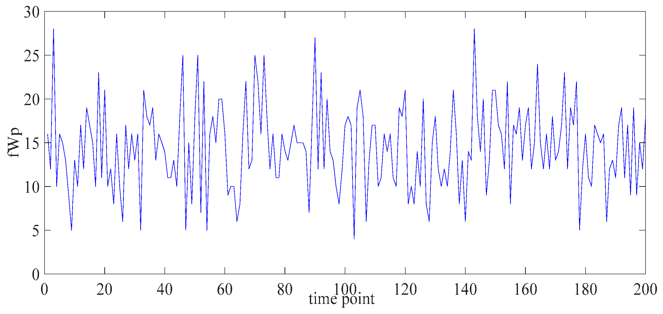
The fWp is a stochastic process based on the fWd, and it thus presents skewed characteristics [6]. We present 200 iterations of the fWp in Figure 2.

2.2. Heavy-Tailed Characteristics and Long-Range Dependence of the fWp

The fWp is proven to exhibit heavy-tailed characteristics and long-range dependence, as follows.

Theorem 1. 

The fWp is heavy-tailed and long-range-dependent.

Proof. 

Random variable $X$ is heavy tailed if the following condition holds:

$$E(e^{\epsilon X})=\infty ,\forall \epsilon >0,$$

(2)

Note that Weibull distribution $X^{\prime }$ has a heavy tail:

$$E(e^{\epsilon X^{\prime }})={\displaystyle \underset{0}{\overset{\infty }{\int }}{e}^{\epsilon x}(\frac{k}{\lambda })}{(\frac{x}{\lambda })}^{k-1}\exp \left\{-{(\frac{x}{\lambda })}^k\right\}dx,$$

(3)

If we signify the fWd as $X^{*}$, then we can reach Equation (4):

$$\begin{array}{l}E(e^{\epsilon X^{*}})={\displaystyle \underset{0}{\overset{\infty }{\int }}{e}^{\epsilon x}(1-\delta )(\frac{k}{\lambda })}{(\frac{x}{\lambda })}^{k-1}\exp \left\{-{(\frac{x}{\lambda })}^k\right\}dx\\ =(1-\delta ){\displaystyle \underset{0}{\overset{\infty }{\int }}{e}^{\epsilon x}(\frac{k}{\lambda })}{(\frac{x}{\lambda })}^{k-1}\exp \left\{-{(\frac{x}{\lambda })}^k\right\}dx\\ =(1-\delta )E(e^{\epsilon X})=\infty ,\forall \epsilon >0.\end{array}$$

(4)

Thus, the fWp is a heavy-tailed random process.

The heavy-tailed characteristics and long-range dependence are equivalent in the temporal domain. Therefore, the fWp is also a long-range-dependent stochastic process. □

2.3. Random Walk Based on fWp

The fWp random walk is associated with its heavy-tailed characteristics [32]. As a heavy-tailed distribution (Theorem 1), the density function of fWd has a heavy tail, which means that the probability for large values is high [33]. Therefore, the jump length is long for the fWp random walk in Figure 3.

Let the initial position of the particle be at the origin. The trajectory of the random walk is described by the coordinates at certain instants of time. In this iteration, a spherical coordinate system is used in which $r$ is the distance between the point and the origin, angle $0\le \theta \le \pi$ is the polar angle of the particle, and $\phi$ is the azimuthal angle ranging within $[0,2\pi ]$. The mathematical expression of the fWp random walk in the ith iteration is as follows:

$$trajectory(i)={(r,\theta ,\phi )}_i~\left\{\begin{array}{c}r~fWd(\lambda ,k,\delta )\\ \theta ~U[0,\pi ]\\ \phi ~U[0,2\pi ]\end{array}\right.i=1,\dots ,n,$$

(5)

3. Difference Iterative Forecasting Model Based on the fWp

3.1. Black–Scholes Model with Long-Range Dependence and Non-Gaussian Characteristics

Previously, Fischer Black and Myron Scholes published the revolutionary paper entitled “The pricing of options and corporate liabilities” [34]. In this paper, the pricing of the stock $S$ is considered to follow the SDE [35]:

$$dS={\mu }^{s}Sdt+{\sigma }^{s}SdB(t),$$

(6)

where ${\mu }^s$ is the expected return rate of the stock, ${\sigma }^s$ is the volatility of the stock, and $B(t)$ is Brownian motion.

The basic assumption for the Black–Scholes model is that the data fluctuation follows Brownian motion. Brownian motion is Markovian; however, real engineering and financial data often possess long memory effects. Brownian motion requires the data to be Gaussian, which indicates a light-tailed and symmetrical data distribution. When the long-range dependence and non-Gaussian characteristics are strong, the modeling effect of the SDE is not satisfactory.

Emphasizing the long-range dependence and non-Gaussian characteristics, e.g., skewness and heavy tail, the fWp is proposed to drive the SDE for the stochastic time series:

$$d(X(t))=\mu X(t)d(t)+\sigma X(t)dfWp(t),$$

(7)

where $\mu$ is the drift coefficient and $\sigma$ is the diffusion coefficient. The drift coefficient regulates the global characteristics, and the diffusion coefficient controls the local variability.

3.2. Stochastic Difference Scheme for the SDE-Based fWp Predictive Model

SDE in Equation (7) can be difficult to solve accurately, thus the difference scheme should be utilized to approximate the true answer [36]. In this section, the numerical solution of the SDE is proposed as the difference iterative prediction model based on the fWp.

The differential of the fWp does not have an analytical expression. Therefore, the Maruyama notation is introduced [37]. The Maruyama notation with the Hurst exponent H is as follows:

$$dfWp(t){=\mathrm{w}}_{\delta }\left(\mathrm{t}\right){(dt)}^H,$$

(8)

where $w_{\delta }$ is white Gaussian noise. In Equation (8), the micro increment of the fWp is transformed to be the actual increment multiplied by a micro increment of time. Let us discretize Equation (8):

$$\Delta fWp(t){=\mathrm{w}}_{\delta }(t){(\Delta t)}^H,$$

(9)

We discretize Equation (7) and combine it with Equation (9):

$$\Delta X(t)=\mu X(t)\Delta t+\sigma X(t)w_{\delta }(t){(\Delta t)}^H,$$

(10)

We set $\Delta t$ to be one prediction time step and the prediction time point is $i$:

$$\Delta X(i)=\mu X(i)+\sigma X(i)w_{\delta }(i)=X(i)(\mu +\sigma w_{\delta }(i)),$$

(11)

Therefore, a difference iterative prediction model is constituted:

$$X(i+1)=X(i)+\Delta X(i)=X(i)+\mu X(i)+\sigma X(i)w_{\delta }(i),$$

(12)

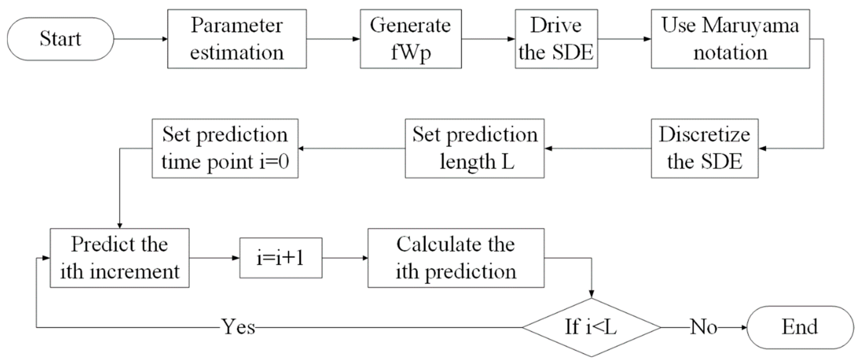
The flow chart is plotted in Figure 4. Engineering data are used to generate the fWp, and then the fWp is employed as the drive force for the SDE of prediction. The SDE is discretized after the Maruyama notation is utilized. At each of the prediction stages, the increment between the present time point and the next time point is predicted. The next point is forecast as the addition of the present value and the increment.

3.3. Parameter Estimation

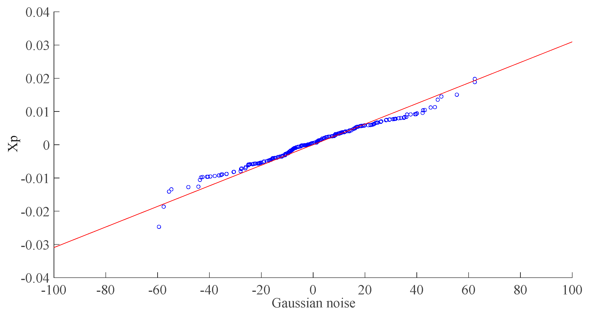
The parameter estimation for the fWp is based on the maximum likelihood estimation in [6]. In this work, we present the estimation method for the drift and diffusion coefficients. This defines a new variable $X_p$, which refers to the proportion of the increments in the stochastic time series.

$$X_P(i)=\frac{\Delta X(i)}{X(i)},$$

(13)

We substitute definition (13) for Equation (11):

$$X_P(i)=\mu +\sigma w_{\delta }(i),$$

(14)

Therefore, the estimation of the drift and diffusion coefficients can be considered as a linear regression based on the least square method.

If we define a deviation function and let the partial derivatives of $\mu$ and $\sigma$ equal zero, we obtain the following:

$$E(\mu ,\sigma )={\displaystyle \sum _{i=1}^n{(X_P(i)-\sigma w_{\delta }(i)-\mu )}^2},$$

(15)

$$\frac{\mathsf{\partial }E(\mu ,\sigma )}{\mathsf{\partial }\mu }={\displaystyle \sum _{i=1}^n\left\{2\mu -2X_P(i)+2\sigma w_{\delta }(i)\right\}}=2n\mu -2{\displaystyle \sum _{i=1}^n{X}_P(i)}+2\sigma {\displaystyle \sum _{i=1}^n{w}_{\delta }(i)}=0,$$

(16)

$$\begin{gathered} \frac{\mathsf{\partial }E(\mu ,\sigma )}{\mathsf{\partial }\sigma }={\displaystyle \sum _{i=1}^n\left\{2{(w_{\delta }(i))}^2\sigma -2X_P(i)w_{\delta }(i)+2\mu w_{\delta }(i)\right\}} \\ =2\sigma {\displaystyle \sum _{i=1}^n{w}_{\delta }{(i)}^2-2{\displaystyle \sum _{i=1}^n{X}_P(i)w_{\delta }(i)+2\mu {\displaystyle \sum _{i=1}^n{w}_{\delta }(i)}}}=0, \end{gathered}$$

(17)

Thus, we can obtain the estimated values of $\mu$ and $\sigma$.

$$\widehat{\sigma }=\frac{n{\displaystyle \sum _{i=1}^n{X}_P(i)w_{\delta }(i)-{\displaystyle \sum _{i=1}^n{X}_P(i){\displaystyle \sum _{i=1}^n{w}_{\delta }(i)}}}}{n{\displaystyle \sum _{i=1}^n{w}_{\delta }{(i)}^2-{({\displaystyle \sum _{i=1}^n{w}_{\delta }(i)})}^2}},$$

(18)

$$\widehat{\mu }=\frac{1}{n}{\displaystyle \sum _{i=1}^n{X}_P(i)}-\frac{n{\displaystyle \sum _{i=1}^n{X}_P(i)w_{\delta }(i){\displaystyle \sum _{i=1}^n{w}_{\delta }(i)-{\displaystyle \sum _{i=1}^n{X}_P(i){({\displaystyle \sum _{i=1}^n{w}_{\delta }(i)})}^2}}}}{n^2{\displaystyle \sum _{i=1}^n{(w_{\delta }(i))}^2-n{({\displaystyle \sum _{i=1}^n}{w}_{\delta }(i))}^2}},$$

(19)

A demonstration of the linear regressive parameter estimation is provided in Figure 5. The drift coefficient is the vertical intercept, and the diffusion coefficient is the slope.

4. Analysis of the Difference Scheme for the SDE Driven by the fWp

4.1. Consistency of the fWp Predictive Model

The consistency of the model indicates that the difference scheme is approximating the SDE to a certain degree. The definition of the consistency is as follows:

Definition 1. 

The finite stochastic difference scheme $\frac{\Delta (U)}{\Delta t}=G^{*}$ is pointwise consistent with the stochastic differential equation $\frac{d(V)}{dt}=G$, if for any continuously differentiable function $X(t)$ in mean square:

$$\underset{\Delta t\to 0}{\lim }(E{\Vert (\frac{dX(t)}{dt}-G)-(\frac{\Delta X(t)}{\Delta t}-G^{*})\Vert }^2)=0,$$

(20)

where $(n+1)\Delta t=t$.

The consistency of the prediction model is provided in Theorem 2:

Theorem 2. 

The fractional Weibull forecasting model is consistent.

Proof. 

Combine Equations (7) and (8):

$$\frac{dX(t)}{dt}=\mu X(t)+\sigma X(t)w_{\delta }(t){(dt)}^{H-1},$$

(21)

Refer to Equation (10):

$$\frac{\Delta X(t)}{\Delta t}=\mu X(t)+\sigma X(t)w_{\delta }(t){(\Delta t)}^{H-1},$$

(22)

Then, define function $G(t)$:

$$G(t)=(\frac{dX(t)}{dt}-\frac{\Delta X(t)}{\Delta t})+[(\mu X(t)+\sigma X(t)w_{\delta }(t){(\Delta t)}^{H-1})-(\mu X(t)+\sigma X(t)w_{\delta }(t){(dt)}^{H-1})],$$

(23)

The limitation of Equation (23) is

$$\begin{array}{l}\underset{\Delta t\to 0}{\lim }G(t)=\underset{\Delta t\to 0}{\lim }(\frac{dX(t)}{dt}-\frac{\Delta X(t)}{\Delta t})+[(\mu X(t)+\sigma X(t)w_{\delta }(t){(\Delta t)}^{H-1})-(\mu X(t)+\sigma X(t)w_{\delta }(t){(dt)}^{H-1})]\\ =\underset{\Delta t\to 0}{\lim }(\frac{dX(t)}{dt}-\frac{dX(t)}{dt})+[(\mu X(t)+\sigma X(t)w_{\delta }(t){(dt)}^{H-1})-(\mu X(t)+\sigma X(t)w_{\delta }(t){(dt)}^{H-1})]\\ =0,\end{array}$$

(24)

Therefore, the criterion for the consistency is proven as follows:

$$\underset{\Delta t\to 0}{\lim }E{\Vert G(t)\Vert }^2=\underset{\Delta t\to 0}{\lim }E(G^2(t))=E\underset{\Delta t\to 0}{\lim }{G}^2(t)=0,$$

(25)

□

4.2. Stability of the fWp Predictive Model

For stability, a small error in the initial condition causes a small error in the final solution. The error in the unstable system then grows exponentially. The definition of the stability is as follows:

Definition 2. 

The finite stochastic difference scheme for the SDE is stable with respect to a norm in mean square if there exist positive constants and such that

$$E{\Vert X(n+1)\Vert }^2\le K{e}^{\beta t}E{\Vert X(0)\Vert }^2,$$

(26)

where $X(t)$ is the approximated solution of the stochastic difference scheme and $0\le t=(n+1)\Delta t$.

The stability of the difference iterative model is proven in the following:

Theorem 3. 

The fractional Weibull forecasting model is stable.

Proof. 

In view of Equation (12), Equation (27) can be formulated as:

$$\mathrm{X}(\mathrm{n}+1)=X(n)+\mu X(n)+\sigma X(n)w_{\delta }(n)=(1+\mu +\sigma w_{\delta }(n))X(n),$$

(27)

The expectation for the difference solution with respect to a norm in mean square is

$$\begin{array}{l}E{\Vert X(n+1)\Vert }^2=E{(X(n+1))}^2\\ =E[{(1+\mu +\sigma w_{\delta }(n))}^2{(X(n))}^2]\\ =E[{(1+\mu +\sigma w_{\delta }(n))}^2{(1+\mu +\sigma w_{\delta }(n-1))}^2{(X(n-1))}^2]\\ =E[{(1+\mu +\sigma w_{\delta }(n))}^2{(1+\mu +\sigma w_{\delta }(n-1))}^2{(X(n-1))}^2]\\ \le {(1+\mu +\max (\sigma w_{\delta }(i)))}^{2(n+1)}E{(X(0))}^2\\ ={(1+\mu +\max (\sigma w_{\delta }(i)))}^{\frac{2}{\Delta t}(n+1)\Delta t}E{(X(0))}^2\\ ={(1+\mu +\max (\sigma w_{\delta }(i)))}^{\frac{2}{\Delta t}t}E{(X(0))}^2\\ ={(1+\mu +\max (\sigma w_{\delta }(i)))}^{\frac{2}{\Delta t}t}E{\Vert X(0)\Vert }^2,\end{array}$$

(28)

With proper chosen positive parameters $K$ and $\beta$, Equation (29) can easily hold:

$${(1+\mu +\max (\sigma w_{\delta }(i)))}^{\frac{2}{\Delta t}t}={\alpha }^{\theta t}\le K{e}^{\beta t},$$

(29)

Combining Equations (28) and (29), Equation (30) can be reached:

$$E{\Vert X(n+1)\Vert }^2\le K{e}^{\beta t}E{\Vert X(0)\Vert }^2,$$

(30)

and this identity proves the stability of the fWp forecasting model. □

4.3. Convergence of the fWp Predictive Model

In order to make the approximated difference solution of the SDE viable, convergence is required. The convergence of the model means that the approximated difference solution can infinitely approach the true answer of the SDE. The definition of the convergence is as follows:

Definition 3. 

A stochastic difference scheme approximating the stochastic differential equation is convergent in mean square at time t if, as $(n+1)\Delta t=t$:

$$\underset{\Delta t\to 0}{\lim }E{\Vert u(n+1)-v(n+1)\Vert }^2=0,$$

(31)

where $u$ is the solution of the difference scheme and $v$ is the corresponding true answer of the SDE.

The consistent difference scheme is a good approximation of the SDE locally, while the convergent difference scheme is a good approximation of the SDE globally. Therefore, consistency is a necessary condition for a scheme to be convergent, but it is not sufficient. The Lax Equivalence Theorem states the necessary and sufficient condition for convergence. For a consistent finite difference scheme, stability is equivalent to convergence [38].

The convergence of the difference iterative model is proven in the following:

Theorem 4. 

The fractional Weibull forecasting model is convergent.

Proof. 

In Theorems 2 and 3, the stability and consistency of the fractional Weibull difference iterative forecasting model are proven. Considering the Lax Equivalence Theorem as feasible, we can conclude that the finite difference scheme is also convergent to the SDE. □

4.4. Model Comparison for the Stochastic Time Series Prediction

The long memory effect of the proposed SDE-based model originates from the heavy-tailed characteristics and long-range dependence of the fWp, which does not require special parameter specification. As in the statistical model, the prediction process is explainable with statistics, and the calculation cost is affordable in the real engineering scene.

The long memory effect is also related to the fractal phenomenon and fractional calculus. The fractional generalization of the autoregressive integrated moving average model allows for the capture of the long memory effect with parameter $d$. The relationship between parameter $d$ and Hurst exponent $H$ is

$$H=d+\frac{1}{2},$$

(32)

When the condition of $d\in (0,0.5)$ is satisfied, the auto-regressive model is long-range-dependent.

Deep learning can grasp the time dependency of the time series with the representation learning of the deep neural network. The learning process is currently within an unexplainable black box. Compared with the explainable statistical approach, the computational complexity is much higher, which affects the prediction accuracy of the small sample learning case.

5. Case Study of Wind Speed Forecasting

All simulations are implemented using MATLAB R2020a on a Lenovo Intel Core-i7-13700, and this computational tool will be used throughout Section 5 and Section 6.

5.1. Data Preprocessing for the Wind Speed Training Dataset

In order to control wind power generation in the new energy power system, future wind speed should be forecast [39]. Wind speed data from Nanjing in 2017 is employed in the current case study, and these are plotted in Figure 6. The augmented Dickey–Fuller test reveals that the training set is not stationary [40].

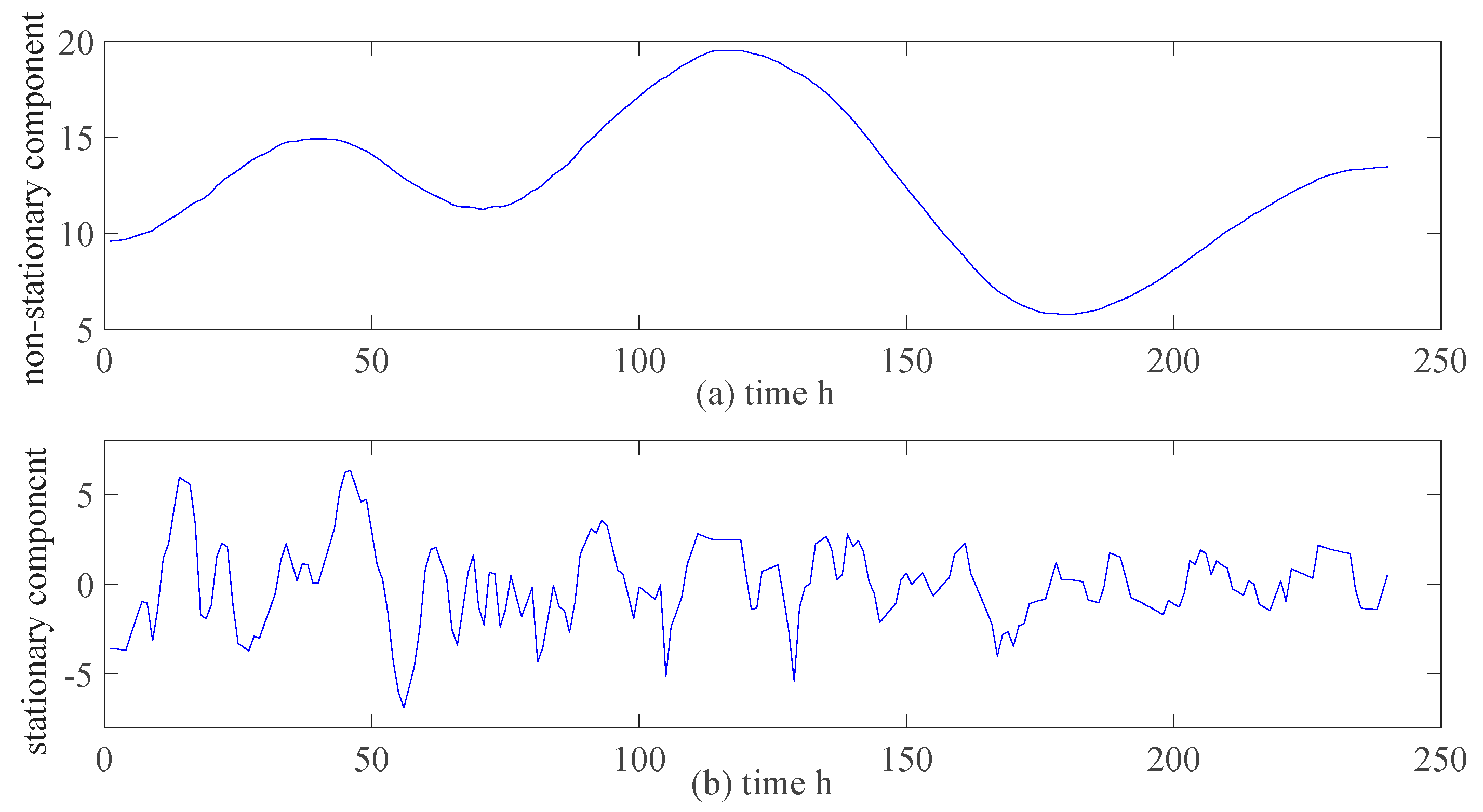
VMD is performed on the training set to separate the stationary and non-stationary components. As we see from Figure 7, the non-stationary component represents a global trend, which conveys most of the information. The non-stationary component should be utilized for the generation of the fWp. The stationary component is the local uncertainty, which represents the wind speed variation on the basis of the current fluctuation trend. The stationary component adds uncertain variation to the deterministic trend of the non-stationary component. The mean and variance of the white Gaussian noise in the Maruyama notation are estimated from the stationary component.

5.2. Statistical Properties of the Wind Speed Series

The options for wind speed modeling are commonly Gaussian distribution, Rayleigh distribution, and Weibull distribution [41]. Wind speed series often present skewness and heavy-tailed characteristics [42,43]. Therefore, probability distribution with heavy tail and skewness should be better for the statistical fitting.

To evaluate the suitable fitting distribution quantitatively, goodness of fit (GoF) is employed [44]. The sum of squared error (SSE) and root mean square error (RMSE) are widely used to evaluate the GoF. The smaller values indicate better fitting results for both criteria. The GoF results are summarized in

Table 1. The GoF results from the wind speed data.

	Gaussian	Weibull	Rayleigh	fWd
SSE	0.0102	0.0102	0.8294	0.0098
RMSE	0.0101	0.0101	0.0911	0.0099

, in which we can confirm that the fWd is the best-fitting distribution.

The Hurst exponent $H$ is the measure of long-range dependence. The stochastic time series are long-range-dependent if $H\in (0.5,1)$. The dataset is non-stationary, and thus we utilize the wavelet variance approach [45]. The variance of wavelet coefficients $\mathrm{var}(m)$ is calculated with respect to different scales $m$. Identifying the slope of the best straight line fit over the entire dataset in Figure 8 with 2H + 1 provides an estimate of H = 0.75. While such a value for H is consistent with long-range dependence, there are significant deviations in the data points from the best fit straight line.

5.3. Performance Evaluation of the Wind Speed Prediction

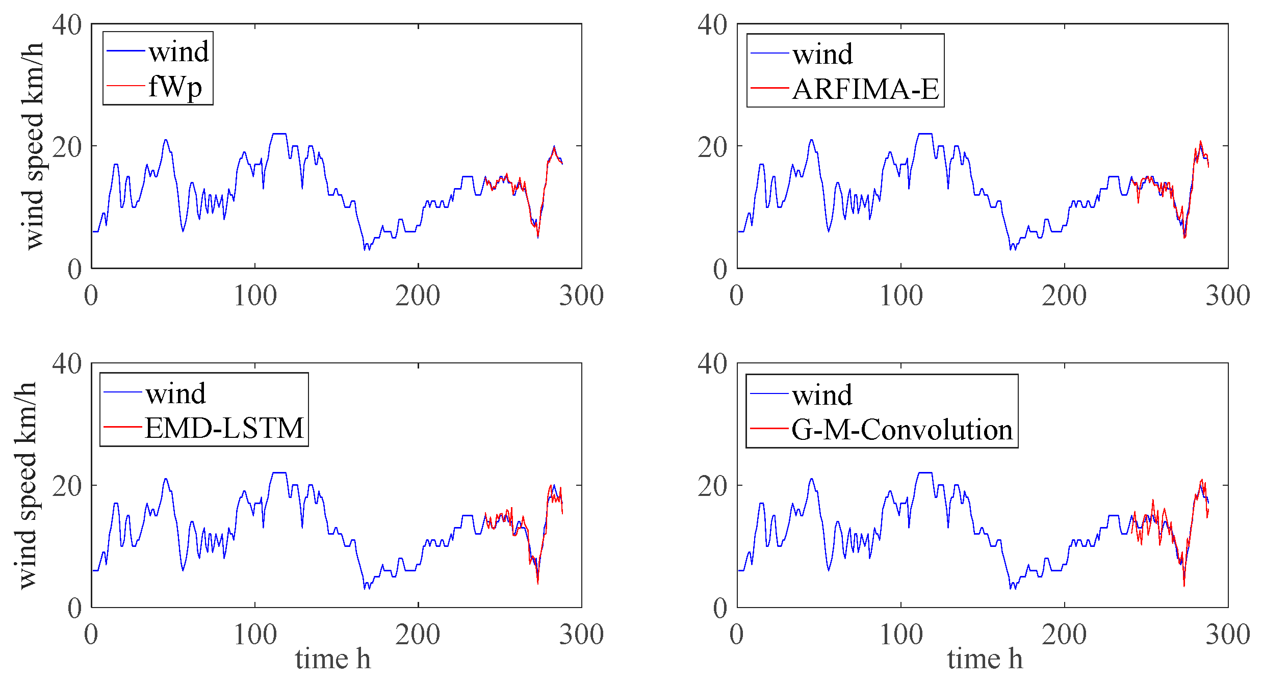
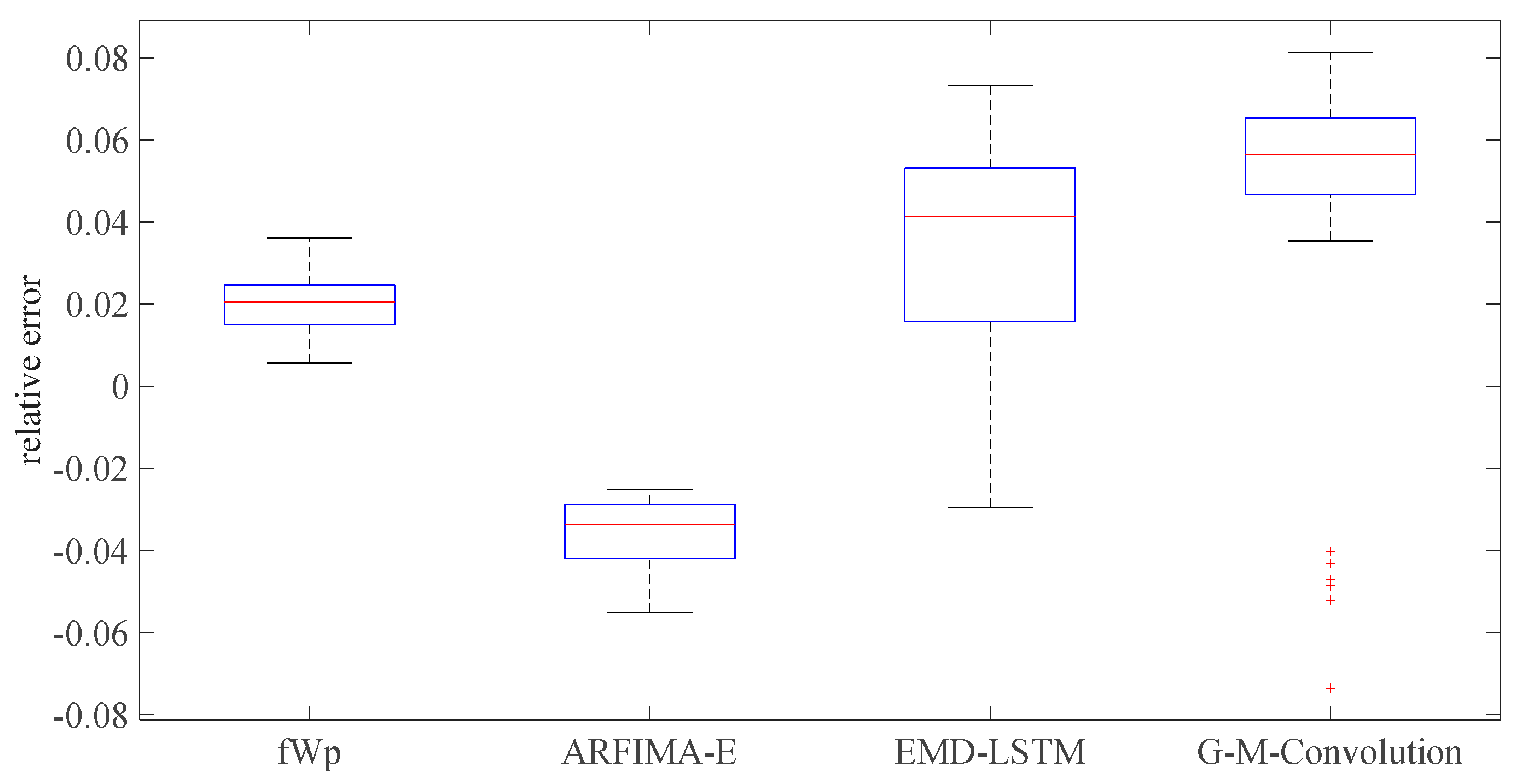
The subsequent 48 h of wind speed data are forecast using the fWp predictive model. The models of the ARFIMA-E, EMD-LSTM, and G-M-Convolution are also utilized for the forecasting. The forecasting results are summarized in Figure 9. The boxplot of the relative prediction errors is depicted in Figure 10.

The traditional statistical metrics of prediction accuracy do not take the random disturbance into consideration. Thus, the Diebold–Mariano test (D-M) is proposed in [46], which is then employed to evaluate the wind speed prediction results in [47]. In this work, the loss differential of the D-M test is:

$$d_t=L(fWp)-L(comparison),$$

(33)

where $L$ is the loss function.

The null hypothesis of the D-M test is that the two models are equally accurate. Since the D-M statistics converge to the standard normal distribution, we can reject the null hypothesis at 5% confidence level if $\left|DM\right|>1.96$. Specifically, the fWp is superior if $DM<-1.96$ and less efficient if $DM>1.96$.

There are two kinds of calculation costs, i.e., the temporal cost and space cost. The floating-point operations (FLOPs) are utilized to analyze the temporal cost [48]. The higher the FLOPs, the larger the temporal cost, which increases the training difficulty. The number of parameters in the model (params) is utilized to evaluate the space cost [49]. The larger the parameter total, the higher the space cost, which increases the difficulty of the engineering application.

The evaluation metrics for the wind speed forecasting are presented in

Table 2. Evaluation metrics for the wind speed forecasting.

	fWp	ARFIMA-E	EMD-LSTM	G-M-Convolution
D-M	0	−2.322	−2.647	−2.934
FLOPs	1923	2362	8.7 × 106	1.02 × 108
params	10	13	4.2 × 106	2.64 × 107

.

6. Case Study of Stock Price Forecasting

6.1. Data Preprocessing for the Stock Price Training Dataset

Stock price forecasting is beneficial for investors to understand the dynamics of asset returns, which enhances the market efficiency. A stock dataset taken from the Shanghai stock market in 2017 is employed in this validation, as depicted in Figure 11.

VMD was used as the data preprocessing algorithm (see Figure 12). The fluctuation trend of the stock price is extracted from the training data, which is the non-stationary component. The stationary component of the stock price series is the variation pattern based on the fluctuation trend.

6.2. Statistical Properties of the Stock Price Series

Gamma distribution, inverse Gamma distribution, and Weibull distribution are commonly used to fit the stock dataset. These probability distributions are skewed and heavy-tailed, which makes them suitable for describing stock price data.

The GoF experiments are conducted to quantitatively determine the best-fitting distribution for the training stock price dataset. As we can see from

Table 3. The GoF results of the stock price data.

	Gamma	Inverse-Gamma	Weibull	fWd
SSE	0.0429 × 10−3	0.2078 × 10−3	0.0264 × 10−3	0.0240 × 10−3
RMSE	0.0007	0.0014	0.0005	0.0005

, the fitting result from the fWd is the best. The wavelet variance approach is utilized for the estimation of the Hurst exponent because the stock price series are not stationary. The Hurst exponent of the stock price dataset is 0.7312, which proves the long-range dependence of the training dataset.

6.3. Performance Evaluation of the Stock Price Prediction

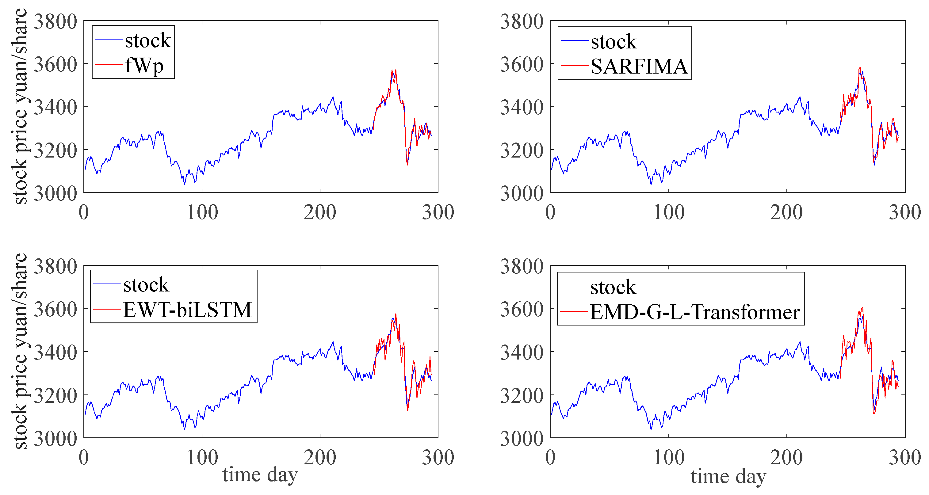
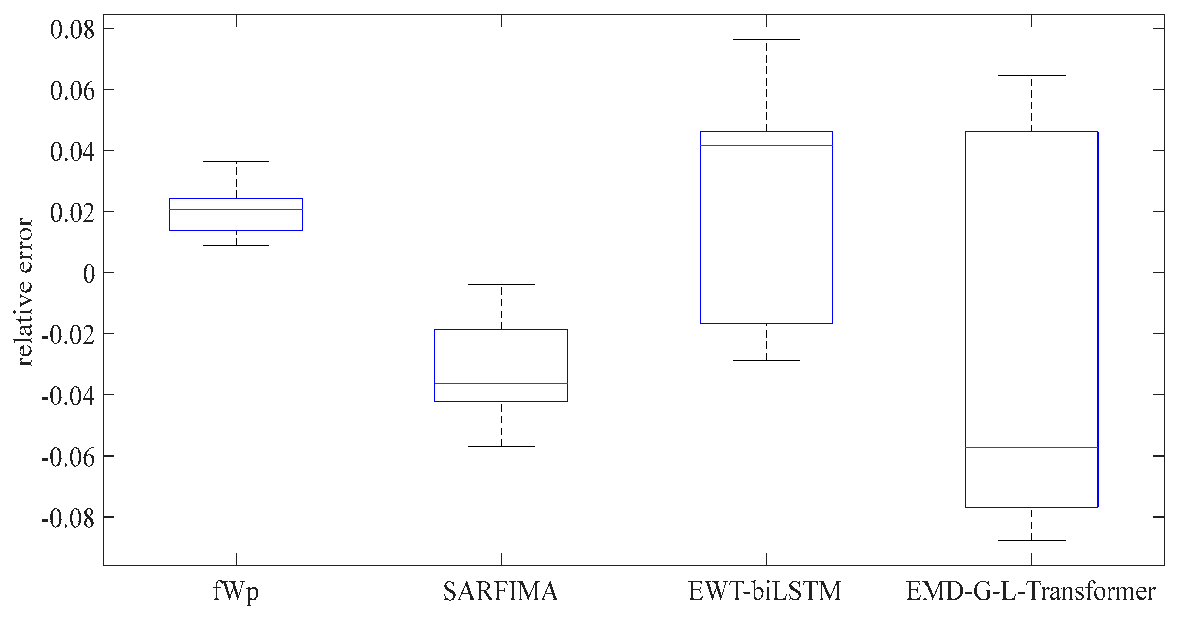
The subsequent 50 days of stock prices are forecast using the fWp predictive model. Three other prediction models are employed as a comparison, i.e., SARFIMA, EWT-biLSTM, and EMD-G-L-Transformer. The prediction results and the boxplot of relative prediction errors are separately plotted in Figure 13 and Figure 14. The prediction accuracy and the calculation cost are also evaluated using the D-M, FLOPs, and params (see

Table 4. Evaluation metrics for the stock price forecasting.

	fWp	SARFIMA	EWT-biLSTM	EMD-G-L-Transformer
D-M	0	−2.368	−2.734	−2.976
FLOPs	2007	4447	9.6 × 106	3.301 × 1018
params	10	24	5.4 × 106	7.6 × 107

).

7. Conclusions

A difference iterative prediction model based on the fWp is proposed as the stochastic difference solution for the improved Black–Scholes model. To facilitate its engineering and financial applications, the stability, consistency, and convergence are proven. The long-range dependence and heavy-tailed characteristics of the fWp are shown to be the mathematical foundation of the predictive model. The skewness of the fWp is also demonstrated. Real wind speed series and stock price series are employed for the validation of the model.

In the future, subsequent research can focus on the extension of the proposed model to the lifetime prediction of other engineering fields.

References

1. Muhammad, A. A study on skewness and kurtosis estimators of wind speed distribution under indeterminacy. Theor. Appl. Climatol. 2021, 143, 1227–1234. [Google Scholar]
2. Park, Y.J. Skewness Versus Kurtosis: Implications for Pricing and Hedging Options. Asia-Pac. J. Financ. Stud. 2017, 46, 903–933. [Google Scholar]
3. Yu, Z.W.; Tuzuzer, A. Fractional Weibull Wind Speed Modelling for Wind Power Production Estimation. In Proceedings of the 2009 IEEE Power & Energy Society General Meeting (PES), Calgary, AB, Canada, 26–30 July 2009. [Google Scholar]
4. Aslam, F.; Latif, S.; Ferreira, P. Investigating Long-Range Dependence of Emerging Asian Stock Markets Using Multifractal Detrended Fluctuation Analysis. Symmetry 2020, 12, 1157. [Google Scholar] [CrossRef]
5. Katikas, L.; Dimitriadis, P.; Koutsoyiannis, D.; Kontos, T.; Kyriakidis, P. A stochastic simulation scheme for the long-term persistence, heavy-tailed and double periodic behavior of observational and reanalysis wind time-series. Appl. Energy 2021, 295, 116873. [Google Scholar] [CrossRef]
6. Deng, W.J.; Song, W.Q.; Cattani, C.; Chen, J.X.; Chen, X.L. On the fractional Weibull process. Front. Phys. 2022, 10, 790791. [Google Scholar] [CrossRef]
7. Bokde, N.; Feijoo, A.; Villanueva, D.; Kulat, K.A. Review on Hybrid Empirical Mode Decomposition Models for Wind Speed and Wind Power Prediction. Energies 2019, 12, 254. [Google Scholar] [CrossRef]
8. Naik, J.; Satapathy, P.; Dash, P.K. Short-term wind speed and wind power prediction using hybrid empirical mode decomposition and kernel ridge regression. Appl. Soft Comput. 2018, 70, 1167–1188. [Google Scholar] [CrossRef]
9. Dragomiretskig, K.; Zosso, D. Variational Mode Decomposition. IEEE Trans. Signal Process. 2014, 62, 531–544. [Google Scholar] [CrossRef]
10. Wang, J.; Liu, Y.; Wu, H.Y.; Lu, S.; Zhou, M. Ensemble FARIMA Prediction with Stable Infinite Variance Innovations for Supermarket Energy Consumption. Fractal Fract. 2022, 6, 276. [Google Scholar] [CrossRef]
11. Hu, H.W.; Zhao, C.N.; Li, J.; Huang, Y.Q. Stock Prediction Model Based on Mixed Fractional Brownian Motion and Improved Fractional-Order Particle Swarm Optimization Algorithm. Fractal Fract. 2022, 6, 560. [Google Scholar] [CrossRef]
12. Czapaj, R.; Kaminski, J.; Soltysik, M. A Review of Auto-Regressive Methods Applications to Short-Term Demand Forecasting in Power Systems. Energies 2022, 15, 6729. [Google Scholar] [CrossRef]
13. Shang, T.; Li, W.Q.; Wu, L. Regional forecasting of wind speed in large scale wind plants. Int. J. Green Energy 2022, 20, 486–496. [Google Scholar] [CrossRef]
14. Bayraktav, E.; Poor, V.H.; Rao, R. Prediction and tracking of long-range -dependent sequences. Syst. Control Lett. 2005, 54, 1083–1090. [Google Scholar] [CrossRef]
15. Feng, S.; Wang, X.M.; Sun, H.W.; Zhang, Y.; Li, L. A better understanding of long range temporal dependence of traffic flow time series. Phys. A Stat. Mech. Appl. 2018, 492, 639–650. [Google Scholar] [CrossRef]
16. Maria, C.M.; Md, A.M.B.; Osei, K.T.; Hector, G.H. Long memory effects and forecasting of earthquake and volcano seismic data. Phys. A Stat. Mech. Appl. 2020, 559, 125049. [Google Scholar] [CrossRef]
17. Liu, K.; Chen, Y.Q.; Zhang, X. An Evaluation of ARFIMA (Autoregressive Fractional Integral Moving Average) Programs. Axioms 2017, 6, 16. [Google Scholar] [CrossRef]
18. Wang, Y.S.; Fang, H.Z.; Jin, J.Y.; Ma, G.J.; He, X.; Dai, X.; Yue, Z.G.; Cheng, C.; Zhang, H.T.; Pu, D.L.; et al. Data-Driven Discovery of Stochastic Differential Equations. Engineering 2022, 17, 244–252. [Google Scholar] [CrossRef]
19. Ali, S.; Abbas, Z.; Butt, M.M. A comparison of different weather forecasting models for the monthly forecast of Lahore city. Mausam 2021, 72, 749–780. [Google Scholar] [CrossRef]
20. Sakthivel, R.; Joby, M.; Anthoni, S.M. Resilient dissipative based controller for stochastic systems with randomly occurring gain fluctuations. Inf. Sci. 2017, 218–419, 447–462. [Google Scholar] [CrossRef]
21. Callado, A.; Kamienski, C.; Szabo, G.; Gero, B.P.; Kelner, J.; Fernandes, S.; Sadok, D. A Survey on Internet Traffic Identification. IEEE Commun. Surv. Tutor. 2009, 11, 37–52. [Google Scholar] [CrossRef]
22. Song, W.Q.; Liu, H.; Enrico, Z. Long-range dependence and heavy tail characteristics for remaining useful life prediction in rolling bearing degradation. Appl. Math. Model. 2022, 102, 268–284. [Google Scholar] [CrossRef]
23. Duan, S.; Song, W.Q.; Zio, E.; Cattani, C.; Li, M. Product technical life prediction based on multi-modes and fractional Lévy stable motion. Mech. Syst. Signal Process. 2021, 161, 107974. [Google Scholar] [CrossRef]
24. Leland, W.E.; Taqqu, M.S.; Willinger, W.; Wilson, D.V. On the Self-Similar Nature of Ethernet Traffic. ACM Sigcomm Comput. Commun. Rev. 1993, 23, 183–193. [Google Scholar] [CrossRef]
25. Shao, B.L.; Song, D.; Bian, G.Q.; Zhao, Y. Wind Speed Forecast Based on the LSTM Neural Network Optimized by the Firework Algorithm. Adv. Mater. Sci. Eng. 2021, 2021, 4874757. [Google Scholar] [CrossRef]
26. Hao, W.; Sun, X.F.; Wang, C.Y.; Chen, H.Y.; Huang, L.M. A hybrid EMD-LSTM model for non-stationary wave prediction in offshore China. Ocean Eng. 2022, 246, 110566. [Google Scholar] [CrossRef]
27. Zhang, X.Y.; Kuenzel, S.; Colombo, N.; Watkins, C. Hybrid Short-term Load Forecasting Method Based on Empirical Wavelet Transform and Bidirectional Long Short-term Memory Neural Networks. J. Mod. Power Syst. Clean Energy 2022, 10, 1216–1228. [Google Scholar] [CrossRef]
28. Song, Y.; Tang, D.Y.; Yu, J.S.; Yu, Z.T.; Li, X. Short-Term Forecasting Based on Graph Convolution Networks and Multiresolution Convolution Neural Network for Wind Power. IEEE Trans. Ind. Inform. 2023, 19, 1691–1702. [Google Scholar] [CrossRef]
29. Li, C.Y.; Qian, G.Q. Stock Price Prediction Using a Frequency Decomposition Based GRU Transformer Neural Network. Appl. Sci. 2023, 13, 222. [Google Scholar] [CrossRef]
30. Abderrahim, Q.; Ernesto, S.M. Generating data from improper distributions: Application to Cox proportional hazards models with cure. J. Stat. Comput. Simul. 2014, 84, 204–214. [Google Scholar]
31. Applebaum, K.M.; Malloy, E.J.; Eisen, E.A. Left Truncation, Susceptibility, and Bias in Occupational Cohort Studies. Epidemiology 2011, 22, 599–606. [Google Scholar] [CrossRef]
32. Sakthivel, R.; Sathishkumar, M.; Kaviarasan, B.; Anthoni, S.M. Synchronization and state estimation for stochastic complex networks with uncertain inner coupling. Neurocomputing 2017, 238, 44–45. [Google Scholar] [CrossRef]
33. Downey, A.B. Lognormal and Pareto Distributions in the Internet. Comput. Commun. 2005, 28, 790–801. [Google Scholar] [CrossRef]
34. Alghalith, M. Pricing the Americanoptions using the Black-Scholes pricing formula. Phys. A Stat. Mech. Appl. 2018, 507, 443–445. [Google Scholar] [CrossRef]
35. Kwok, K.L.; Chiu, M.C.; Wong, H.Y. Demand for longevity securities under relative performance concerns: Stochastic differential games with cointegration. Insur. Math. Econ. 2017, 71, 353–366. [Google Scholar] [CrossRef]
36. Roth, C.H. Difference Methods for Stochastic Partial Differential Equations. ZAMM-Z. Angew. Math. Mech. 2002, 82, 821–830. [Google Scholar] [CrossRef]
37. Liu, L.; Li, M.L.; Deng, F. Stability equivalence between the neutral delayed stochastic differential equations and the Euler-Maruyama numerical Scheme. Appl. Numer. Math. 2008, 127, 370–386. [Google Scholar] [CrossRef]
38. Lang, A. A Lax equivalence theorem for stochastic differential equations. J. Comput. Appl. Math. 2010, 234, 3387–3396. [Google Scholar] [CrossRef]
39. Shi, H.Y.; Dong, Z.B.; Xiao, N.; Huang, Q.N. Wind Speed Distributions Used in Wind Energy Assessment: A Review. Front. Energy Res. 2021, 9, 769920. [Google Scholar] [CrossRef]
40. Paparoditis, E.; Politis, D.N. The asymptotic size and power of the augmented Dickey-Fuller test for a unit root. Econom. Rev. 2018, 37, 955–973. [Google Scholar] [CrossRef]
41. Hu, B.; Li, Y.D.; Yang, H.J.; Wang, H. Wind speed model based on kernel density estimation and its application in reliability assessment of generating systems. J. Mod. Power Syst. Clean Energy 2017, 5, 220–227. [Google Scholar] [CrossRef]
42. Huang, G.Q.; Xia, L.L.; Liu, M.; Wang, D.H.; Zheng, H.T. Tail-Weighted Wind Speed Distribution by Mixture Model with Constrained Maximum Likelihood. Int. J. Struct. Stab. Dyn. 2022, 22, 2240016. [Google Scholar] [CrossRef]
43. Xie, D.F.; Chen, K.S.; Yang, X.F. Effect of Bispectrum on Radar Backscattering From Non-Gaussian Sea Surface. IEEE J. Sel. Top. Appl. Earth Obs. Remote Sens. 2020, 12, 4367–4378. [Google Scholar] [CrossRef]
44. Zheng, H.B.; Huang, W.F.; Zhao, J.H.; Liu, J.F.; Zhang, Y.Y.; Shi, Z.; Zhang, C.H. A normal falling model for wind speed probability distribution of wind farms. Renew. Energy 2022, 184, 91–99. [Google Scholar] [CrossRef]
45. Serroukh, A.; Walden, A.T.; Percival, D.B. Statistical Properties and Uses of the Wavelet Variance Estimator for the Scale Analysis of Time Series. J. Am. Stat. Assoc. 2000, 95, 184–196. [Google Scholar] [CrossRef]
46. Diebold, F.X. Comparing Predictive Accuracy, Twenty Years Later: A Personal Perspective on the Use and Abuse of Diebold-Mariano Tests. J. Bus. Econ. Stat. 2015, 33, 1. [Google Scholar] [CrossRef]
47. Chen, H.; Wan, Q.L.; Wang, Y.R. Refined Diebold-Mariano Test Methods for the Evaluation of Wind Power Forecasting Models. Energies 2014, 7, 4185–4198. [Google Scholar] [CrossRef]
48. Guo, Z.X.; Xiao, Y.F.; Liao, W.Z.; Veelaert, P.; Philips, W. FLOPs-efficient filter pruning via transfer scale for neural network acceleration. J. Comput. Sci. 2021, 55, 101459. [Google Scholar] [CrossRef]
49. Lu, Y.; Lu, G.M.; Li, J.X.; Xu, Y.R.; Zheng, D. High-parameter-efficiency convolutional neural networks. Neural Comput. Appl. 2020, 32, 10633–10644. [Google Scholar] [CrossRef]
Figure 1. Probability density functions of fractional Weibull distribution (fWd) with different skewness (a) and fractal parameter δ (b).
Fractalfract 08 00007 g001
Figure 2. Exemplary trajectory of the fractional Weibull process (fWp).
Fractalfract 08 00007 g002
Figure 3. Random walk based on the fractional Weibull process (fWp).
Fractalfract 08 00007 g003
Figure 4. Flow chart of the fractional Weibull difference iterative prediction model. fWp is short for fractional Weibull process, and SDE stands for stochastic differential equation.
Fractalfract 08 00007 g004
Figure 5. Linear regression for the estimation of drift and diffusion coefficients. X P indicates the proportion of the increments in the stochastic time series.
Fractalfract 08 00007 g005
Figure 6. Training set of the wind speed series.
Fractalfract 08 00007 g006
Figure 7. (a) Non-stationary component of the wind speed series. (b) Stationary component of the wind speed series.
Fractalfract 08 00007 g007
Figure 8. Estimation of the Hurst exponent for the wind speed series. V a r ( m ) is the variance of wavelet coefficient on the scale of m .
Fractalfract 08 00007 g008
Figure 9. Prediction results for the wind speed series.
Fractalfract 08 00007 g009
Figure 10. Boxplot of the wind speed relative prediction errors.
Fractalfract 08 00007 g010
Figure 11. Training set of the stock price series.
Fractalfract 08 00007 g011
Figure 12. (a) Non-stationary component of the stock price series. (b) Stationary component of the stock price series.
Fractalfract 08 00007 g012
Figure 13. Prediction results for the stock price series.
Fractalfract 08 00007 g013
Figure 14. Boxplot of the stock price relative prediction errors.
Fractalfract 08 00007 g014