Article

Pore Structure Characterization and Fractal Analysis of Lacustrine Shales: Integrating N2 Adsorption, Mercury Intrusion, and Deep Learning-Assisted FIB–SEM 3D Pore Surface Point Cloud Reconstruction

1
College of Computer Science and Technology, China University of Petroleum (East China), Qingdao 266580, China
2
Center of Deep Sea Research, Institute of Oceanology, Chinese Academy of Sciences, Qingdao 266071, China
3
School of Geosciences, China University of Petroleum (East China), Qingdao 266580, China
*
Authors to whom correspondence should be addressed.
Fractal Fract. 2026, 10(3), 179; https://doi.org/10.3390/fractalfract10030179
Submission received: 14 January 2026 / Revised: 24 February 2026 / Accepted: 3 March 2026 / Published: 11 March 2026

Abstract

Lacustrine shales are key targets for shale oil exploration, yet the quantitative characterization of their complex and heterogeneous pore systems remains a significant challenge, constraining effective reservoir evaluation and development. This study investigates lacustrine shales from the Second Member of the Kongdian Formation by integrating N2 adsorption, mercury intrusion porosimetry, and focused ion beam scanning electron microscopy with fractal analysis. A Mamba-based deep learning model was applied to improve two-dimensional (2D) pore segmentation, and three-dimensional (3D) pore surface point clouds were reconstructed for 3D surface fractal characterization to reduce artifacts associated with conventional 3D reconstruction. The results indicate that the pore system is dominated by inorganic pores, mainly irregular interparticle pores and dissolution pores, while organic pores are scarce. Pore sizes are predominantly concentrated in the range of 5 to 200 nm. Adsorption-derived fractal dimensions exhibit systematic lithofacies differences, with D1 and D2 averaging around 2.47 and 2.56, respectively. These trends are consistent with the 3D pore surface fractal dimension derived from pore surface point clouds (mean 2.48), which supplements the bulk statistical results with direct geometric quantification of surface roughness. The heterogeneity of the pore system is influenced by the coupled effects of mineral composition, organic matter content, and diagenesis. Specifically, the enrichment of clay minerals and dolomite increases the irregularity of pore morphology and results in higher fractal dimensions. In contrast, samples enriched in feldspars and calcite are supported by a rigid granular framework that corresponds to lower 3D surface complexity. Ultimately, these fractal dimensions effectively quantify pore network complexity and reservoir heterogeneity in the Kong 2 shales, offering quantitative support for reservoir characterization and lacustrine shale oil exploration.

1. Introduction

In recent years, shale systems have been increasingly recognized as a primary target of unconventional hydrocarbon exploration, with extensive progress in play evaluation and development across North America, China, and North Africa [1,2,3]. In China, lacustrine shale successions host substantial shale oil resources [4,5]. Yet, compared with marine shale systems, lacustrine shale reservoirs are commonly more heterogeneous because the typically smaller water volumes and hydrologically sensitive lake basins render sedimentation and early diagenesis highly responsive to environmental fluctuations [6,7], leading to strong lithofacies variability and complex pore architectures. Consequently, reservoir evaluation and development are frequently hindered by complex pore structure, strong pore system heterogeneity, and limited effective connectivity [4,8].
The complex architecture of the pore system governs petrophysical properties and hydrocarbon mobility, making systematic characterization essential for mechanistic interpretation and reservoir evaluation [9,10]. Shale pore systems can be characterized using complementary approaches, ranging from SEM imaging that directly documents pore types and morphologies to multiscale laboratory measurements [11,12], including low-temperature N2/CO2 adsorption, high-pressure mercury intrusion (MIP), nuclear magnetic resonance (NMR), and small-angle neutron scattering (SANS), which quantify pore size distributions, specific surface area (SSA), and related attributes over complementary scale ranges [13,14]. Collectively, these methods have been widely applied not only in shale reservoir studies but also in other unconventional reservoirs and heterogeneous geomaterials (e.g., coal and geothermal crystalline rocks), providing quantitative constraints on pore structure properties across materials [15,16,17]. Furthermore, integrating multiscale experiments with machine learning has proven highly effective for evaluating complex, heterogeneous mixtures [18,19].
Although conventional methods can provide reliable constraints on pore geometry and size distributions, each technique has its own strengths and limitations and is sensitive to different pore domains and scale ranges; therefore, a combined, multi-technique workflow is needed for reliable pore structure characterization. For example, adsorption mainly reflects adsorption-accessible pores, whereas MIP is throat-controlled, and their pore size metrics are not directly interchangeable. In addition, many conventional measurements rely on two-dimensional (2D) sections or bulk averages, which limits the direct quantification of three-dimensional (3D) spatial organization and topological connectivity [3,14,15]. 3D imaging approaches, including FIB-SEM and X-ray micro/nano-computed tomography (micro-CT/nano-CT), enable the direct visualization of pore space and quantitative characterization of pore geometry, including pore shape and surface complexity, connectivity and topology including connected components, percolation pathways, and bottlenecks, as well as spatially resolved heterogeneity within microstructural domains [19,20]. Moreover, 3D reconstructions provide a physical basis for digital rock simulations and for geometry-based characteristics including surface roughness and fractal descriptors. Therefore, 3D structure-based, visualization-enabled quantification is essential for the comprehensive characterization of shale pore systems.
FIB–SEM serial sectioning provides nanoscale images of microstructures and voxel-based, volume-resolved 3D imaging, enabling the direct observation and quantification of nanopores as well as their spatial relationships with organic matter and mineral phases [21,22]. However, accurate quantitative analysis based on FIB–SEM slices is highly dependent on image segmentation quality. Conventional image segmentation processing workflows (e.g., global/adaptive thresholding, watershed segmentation, and edge-detection schemes) typically require extensive manual parameter tuning and remain sensitive to illumination variability, imaging artifacts, and noise, and they are particularly challenged by pores embedded in texturally complex backgrounds and by irregular, multiscale pore morphologies [23]. U-Net, a widely used convolutional neural network (CNN) architecture designed for semantic segmentation, can learn semantic features beyond grayscale intensity and gradients when trained on sufficient datasets. This allows it to outperform traditional methods in the accuracy of shale pore segmentation [24,25]. However, CNNs are restricted by the locality of convolution operations, with the expansion of the effective receptive field depending heavily on the repeated downsampling of feature maps, these architectures tend to miss elongated and slit-shaped pore structures, often resulting in fragmented or incomplete segmentation [26]. In contrast, the Mamba [27] deep learning model based on state space models (SSMs) [28] can capture long-range dependencies and integrate both local and global context, facilitating the delineation of continuous elongated and slit-shaped pores [29]. However, they struggle with small obliquely oriented pores that appear as tiny isolated closed loops in 2D slices [30]. To address this limitation, this study proposes an improved variant of SCSegamba [31] that exploits inter-slice spatial context from adjacent FIB–SEM slices to mitigate the omission of oblique pores in 2D images.
Following precise segmentation, conventional workflows typically generate 3D voxel volume or surface mesh through 3D reconstruction [32], on which quantitative analyses are performed, including pore size distributions, connectivity metrics, permeability evaluation, and fractal analysis. Fractal theory, initially proposed by Mandelbrot in 1967 [33], provides a robust statistical framework for describing the irregularity and self-similarity of complex porous media. It quantitatively characterizes intrinsic surface roughness and structural complexity through the fractal dimension (D) [34,35], establishing a solid foundation for reservoir quality assessment [36,37,38]. Recent studies have applied the box-counting method to SEM or CT reconstructions to spatially quantify geometric complexity [39,40]. However, traditional voxel or mesh 3D reconstruction workflows typically involve resampling, interpolation, and smoothing, which may introduce hard-to-quantify artifacts and thus compromise the accuracy of 3D fractal analysis [41]. This issue mainly arises because surface-based fractal quantification is highly sensitive to the precision of pore boundary reconstruction: these processing steps not only modify small-scale surface undulations but may also artificially regularize pore boundaries, reducing surface roughness. Although such effects are often negligible for visualization or coarse-scale metrics, they can be disproportionately amplified in 3D surface fractal analysis, potentially leading to underestimated fractal dimensions. To mitigate this reconstruction-induced bias, this study proposes an alternative strategy: constructing a 3D pore surface point cloud directly from high-quality 2D pore masks segmented from FIB–SEM slices. Since this point cloud representation obviates the need for additional surface regularization, it maximally preserves the original pore surface morphology, thereby providing a more direct and accurate geometric basis for 3D fractal characterization. In parallel to image-based methods, recent studies frequently utilize the Frenkel–Halsey–Hill (FHH) model based on gas adsorption isotherms to characterize the bulk rugosity of pore surfaces [42,43]. However, adsorption-derived fractals provide bulk-averaged signals without spatial attribution, whereas image-based 3D fractals are restricted to small, potentially non-representative micro-volumes. To bridge this scale and modality gap, this study integrates the FHH model with a point cloud-based 3D box-counting method. Rather than forcing a direct numerical linkage, this dual approach pairs bulk adsorption-derived fractal responses with spatially explicit pore surface complexity as complementary constraints. This mutually informing framework provides a more comprehensive, cross-scale understanding of pore system heterogeneity, helping to mitigate scale-related interpretational ambiguity in lithofacies-scale reservoir evaluation.
Accordingly, this study investigates the lacustrine shales from the Second Member of Kongdian Formation (Kong 2) in the Bohai Bay Basin, China. By employing an integrated workflow that combines X-ray diffraction (XRD), bulk geochemical analyses, SEM, low-pressure N2 adsorption (LPNA), MIP, and fractal analysis, this research systematically characterizes pore types, pore morphologies, SSA, and pore size distributions, and evaluates the fractal heterogeneity of the pore structure across various lithofacies. Furthermore, 3D pore surface point clouds were constructed from FIB-SEM slices using a deep learning segmentation model and a neighborhood-based boundary identification algorithm, followed by box-counting fractal analysis to quantify pore surface complexity. The objectives are to: (1) quantify multiscale pore structures across lithofacies; (2) quantify fractal heterogeneity and its controlling factors; and (3) improve the accuracy of 3D pore structure characterization from FIB–SEM data. Overall, this work refines a quantitative framework for multiscale pore structure characterization in lacustrine shales and improves the mechanistic understanding of pore system heterogeneity and its controlling factors. It provides geologically grounded constraints for sweet spot identification and reservoir quality prediction in terrestrial shale oil exploration and development, and may also serve as a methodological reference for pore structure characterization in other heterogeneous geomaterials.

2. Geological Setting

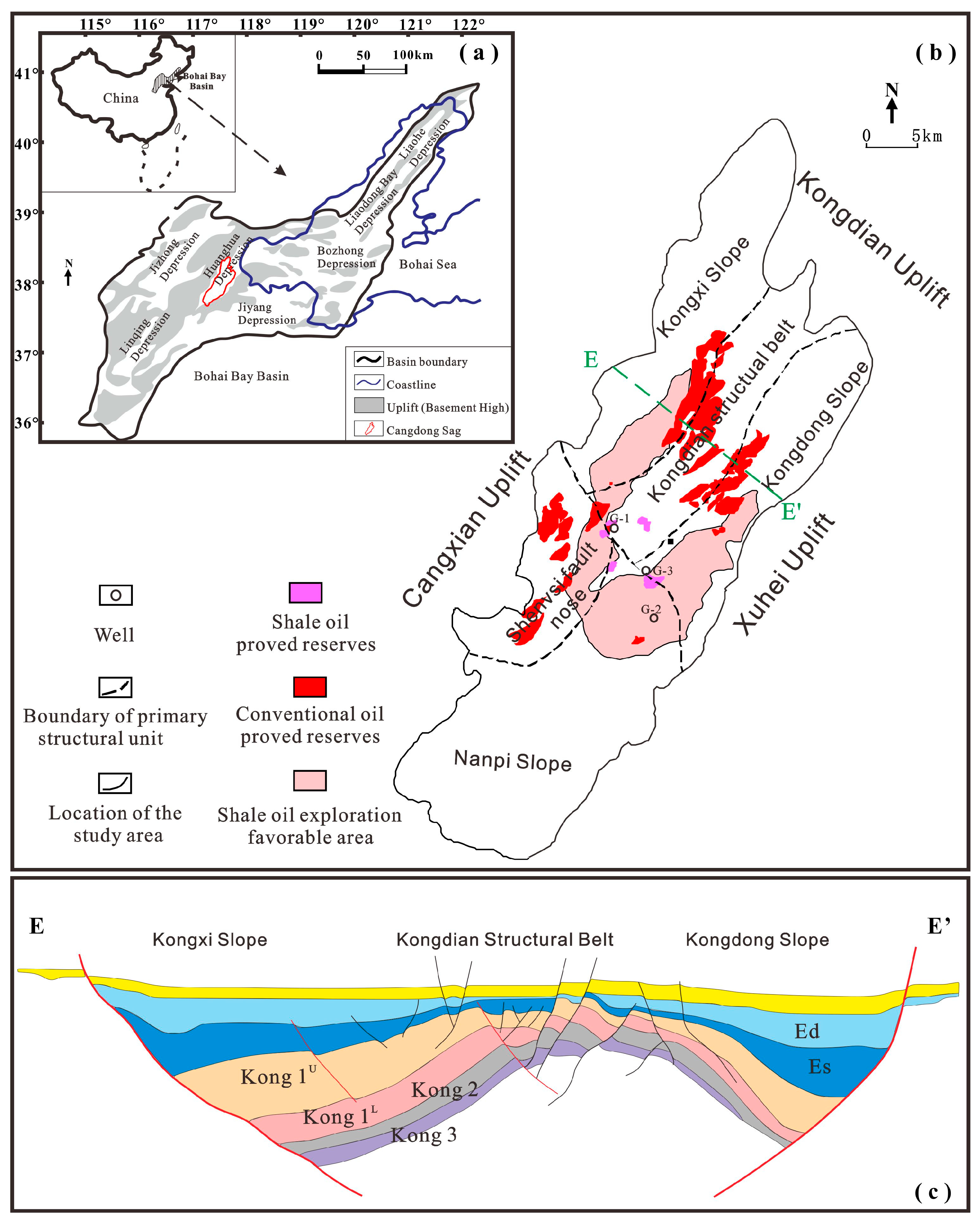
The Bohai Bay Basin is a Cenozoic rift system in eastern North China. Within the central Bohai Bay Basin, the Huanghua Depression contains several hydrocarbon-bearing sub-depressions, among which the Cangdong Sag is a key depocenter for Paleogene lacustrine successions [44]. The Cangdong Sag trends NNE and is flanked by surrounding structural highs, bounded by the Cangxian Uplift to the west, the Xuhei Uplift to the east, and the Kongdian Uplift to the northeast (Figure 1). Two major boundary faults, the Cangdong Fault along the western margin and the Xuxi Fault along the eastern margin, define the primary structural framework controlling subsidence and accommodation in the sag [44,45]. Internally, the sag is further partitioned into multiple secondary structural units, including the Kongxi Slope, Kongdian Structural Belt, Kongdong Slope, Nanpi Slope, and the Shenvsi Fault Nose Belt [44,46].
The Cenozoic evolution of the Cangdong Sag is commonly described as a rift–sag tectonostratigraphic evolution, with Paleogene syn-rift deformation followed by Neogene post-rift thermal subsidence [47,48]. Early Paleogene extension created accommodation controlled by fault activity and promoted lacustrine deposition, locally accompanied by volcanic activity. The subsequent weakening of fault activity and progressive regional subsidence during the Neogene led to a broader, more stable post-rift depression [24]. Stratigraphically, the Paleogene fill of the Cangdong Sag comprises, in ascending order, the Kongdian (Ek), Shahejie (Es), and Dongying (Ed) Formations [48,49] (Figure 1c).
Figure 1. Geological setting of the Cangdong Sag, Bohai Bay Basin. (a) Location and basin-scale tectonic framework. (b) Structural map of the Cangdong Sag with wells, oil occurrences, and shale oil favorable area (after [46,49]). (c) Generalized stratigraphic–structural section E–E′ across the sag.
Fractalfract 10 00179 g001
The Kongdian Formation is subdivided into three members, among which the second member (Kong 2) represents the principal organic-rich shale interval targeted for shale oil exploration. The Kong 2 is characterized by regionally extensive fine-grained lacustrine deposits, dominated by dark shale with interbeds of calcareous shale, and is further divided into four sub-members stratigraphically [44,46]. Long-term exploration has confirmed widespread shale development in the study area, with numerous wells reporting hydrocarbon shows and successful oil tests in selected horizons [49].

3. Materials and Methods

A total of 40 core samples were collected from the Cangdong Sag, Bohai Bay Basin. All samples were subjected to a consistent suite of bulk analyses, including whole rock XRD, TOC determination, and Rock-Eval pyrolysis, to constrain mineralogical and geochemical backgrounds. Subsets were then selected for pore structure characterization: 40 samples for low-pressure N2 adsorption (LPNA), 15 samples for MIP and SEM observations, and 4 representative samples for FIB–SEM analysis.

3.1. Bulk Geochemistry and Mineralogy

TOC measurements were performed using a LECO CS-744 analyzer (LECO Corporation, St. Joseph, MI, USA). Samples were ground to a 100-mesh powder. To remove inorganic carbon, a portion of each sample was treated with 10% (v/v) HCl for 24 h, then rinsed with deionized water until neutral, dried, and combusted under a stream of oxygen to quantitatively determine the organic carbon content.
Rock-Eval pyrolysis analysis was performed on the same powdered samples using a Rock-Eval 7 instrument (Vinci Technologies, Nanterre, France), following standard procedures. Approximately 80 mg of each sample was analyzed under an inert atmosphere to obtain S1, S2, Tmax, and derived indices such as HI (S2 × 100/TOC).
Whole-rock mineral composition was determined through X-ray diffraction (XRD) using a Bruker AXS D8-Focus diffractometer (Bruker AXS SE, Karlsruhe, Germany) (CuKα radiation, 40 kV, 40 mA, Ni filter). Powdered samples (<75 μm) were scanned in the 3–70° (2θ) range with a step size of 0.02°. Semi-quantitative mineral content was estimated using MDI Jade 5.0 software.

3.2. Low-Pressure N2 Adsorption (LPNA)

3.2.1. Measurements

Low-pressure N2 adsorption measurements were performed on 40 representative samples using a Micromeritics ASAP 2460 surface area and porosity analyzer (Micromeritics Instrument Corporation, Norcross, GA, USA) at 77.3 K. The samples were gently crushed and sieved to 40–60 mesh to minimize the influence of macroscopic fractures while ensuring adequate gas accessibility. Prior to analysis, the samples were oven-dried at 60 °C for at least 48 h and subsequently degassed under vacuum at 60 °C for 24 h to remove moisture and adsorbed volatiles.
Adsorption–desorption isotherms were collected over a relative pressure range of P/P0 = 0.002–0.993. The SSA was calculated using the Brunauer–Emmett–Teller (BET) method [50] over the linear region of the BET plot. Pore size distributions (PSD) and pore volumes in the mesopore range were derived using the Barrett–Joyner–Halenda (BJH) method [51].

3.2.2. Fractal Theory Based on LPNA

Fractal concepts have been extensively used to describe the scale-dependent heterogeneity of porous media as revealed by gas adsorption. In particular, the adsorption-based fractal framework proposed by Pfeifer and Avnir [52] provides a convenient way to quantify pore surface complexity from low-temperature N2 isotherms, where the fractal dimension D serves as a descriptor of surface roughness and structural heterogeneity. Shales, as complex multicomponent porous systems, often exhibit fractal-like adsorption behavior over specific pressure ranges and can therefore be characterized using adsorption-derived fractal metrics. Accordingly, fractal characteristics of adsorption-accessible pore surfaces were evaluated in this study from low-temperature N2 isotherms using the Frenkel–Halsey–Hill (FHH) model interpreted within the Pfeifer–Avnir fractal framework. For each sample, the adsorption branch was used to construct the FHH plot, and the adsorption amount V was related to the relative pressure P0/P as follows:
ln V = C + K ln [ln(P0/P)],
where V is the adsorbed volume (cm3 STP g−1), P is the equilibrium pressure, P0 is the saturation vapor pressure of N2 at 77.3 K, C is a constant, and K is the slope obtained from the least-squares linear regression of the FHH plot over the selected relative-pressure interval. Under the Pfeifer–Avnir interpretation, the fractal dimension D is obtained from
D = K + 3,
with D theoretically ranging between 2 and 3, where values closer to 2 indicate a relatively smoother surface and values approaching 3 imply increased surface roughness and heterogeneity.
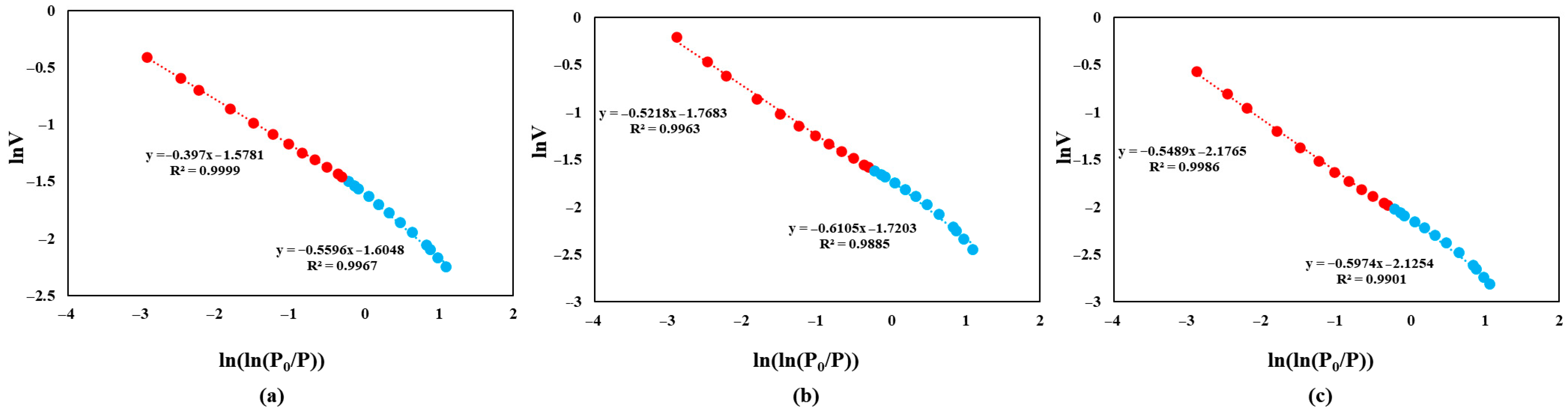
Because shale isotherms commonly exhibit scale-dependent behavior, the FHH plot was examined for quasi-linear segments. When two distinct linear regimes were present, two fractal dimensions were reported (D1 and D2). To improve reproducibility and inter-sample comparability while allowing for sample-to-sample differences, the fitting-window search was constrained to two physically meaningful relative-pressure domains separated by a transition zone around P/P0 ≈ 0.47–0.50, excluding the near-saturation region where capillary condensation and hysteresis may bias linearity. Within each domain, candidate continuous sub-intervals were tested, and the sub-interval yielding the best linear regression was retained. As a quality-control criterion, only regressions with R2 > 0.90 were accepted. Furthermore, to quantify the uncertainty of the derived fractal dimensions, the standard error (SE) of the linear regression slope was calculated for each sample (SE(D) = SE(K)). The sample-by-sample P/P0 fitting ranges and regression statistics are provided. In addition, a window-sensitivity check was performed by perturbing the fitted bounds by ±5% of the selected window width in P/P0 and recalculating D1 and D2, which yielded minor variations in the computed fractal dimensions.

3.3. Mercury Intrusion Porosimetry (MIP)

High-pressure MIP was conducted on 15 cube-shaped samples (approximately 1 cm × 1 cm × 1 cm) using a mercury porosimeter, following GB/T 21650.1-2008 [53]. Prior to analysis, samples were dried at 60 °C for 48 h and cooled in a desiccator to room temperature. Intrusion pressure was increased stepwise from 0.034 MPa to 413 MPa, and pore-throat size was calculated using the Washburn equation [54], with instrument-standard values for mercury surface tension and contact angle consistent with the GB/T protocol. The measurable pore size range spans approximately 3 nm to 300 μm.

3.4. Focused Ion Beam Scanning Electron Microscopy (FIB-SEM)

Shale sample blocks with a thickness of 5 mm and dimensions of 10 mm in length and width were prepared. The surface of the sample blocks was polished using an argon ion beam to ensure a smooth surface. Conductive silver paste was then applied to the four sides and bottom of the polished samples to reduce charge accumulation on the sample surface and improve imaging quality. 3D pore architectures were reconstructed by serial sectioning using a ZEISS Crossbeam 550 dual-beam FIB–SEM system (Carl Zeiss, Jena, Germany). Representative regions (30 μm × 30 μm × 30 μm) were selected for tomographic acquisition. The specimen stage was tilted to 54° to achieve coincidence geometry between the ion and electron columns, followed by beam alignment and focusing. A trapezoidal trench was milled using a Ga+ ion beam operated at 30 kV and 65 nA to expose the imaging cross-section. To improve milling stability and reduce curtaining effects, auxiliary side trenches were excavated at 30 kV and 30 nA. The exposed cross-section was subsequently subjected to sequential coarse and fine ion-beam polishing using reduced beam currents to obtain a flat imaging surface. Serial slicing was performed for 2000 cycles. In each cycle, a 15 nm thick layer was removed using a 30 kV, 7 nA Ga+ ion beam, and the freshly exposed surface was imaged through SEM at 1 kV and 500 pA. SEM images were acquired using multiple detectors, including secondary electron (SE), InLens, and backscattered electron (BSE) modes, to maximize pore–matrix contrast and preserve microstructural details. The pre-milling and polishing steps required approximately 10 h, and the subsequent serial sectioning and imaging required approximately 20 h. After acquisition, each SEM slice was cropped to a central region of interest (ROI) to generate 2000 × 2000-pixel images.

3.5. 2.5D SCSegamba Framework for FIB–SEM Pore Segmentation

This study developed an enhanced 2.5D SCSegamba segmentation framework by extending the SCSegamba network [39]. The model is built upon the Vision Mamba architecture [55], overcoming the inherent local receptive field limitations of traditional convolutional neural networks (CNNs). By leveraging the linear complexity of Mamba’s selective state-space scanning [56], it enables effective modeling of long-range dependencies across the entire image at a low computational cost. In SCSegamba, the Structure-Aware Scanning Strategy (SASS) is designed as the scan-ordering scheme for the 2D selective scan (SS2D) within the Structure-Aware Visual State Space (SAVSS) block, aiming to preserve the semantic continuity of narrow, elongated, and multi-directional structures during sequence modeling.
As illustrated in Figure 2, the 2D token grid is serialized through four complementary snake-style routes: two parallel snake paths (a column-wise serpentine traversal and a row-wise serpentine traversal) and two diagonal snake paths (serpentine traversals along the two diagonal orientations). By constructing these multi-directional adjacency relationships, SASS ensures that successive tokens in each scan are spatially adjacent along a plausible pore propagation direction, enabling the state-space recurrence to propagate contextual cues more consistently across regular and oblique or interwoven textures, thereby better capture complex pore morphologies under cluttered backgrounds while remaining computationally efficient.
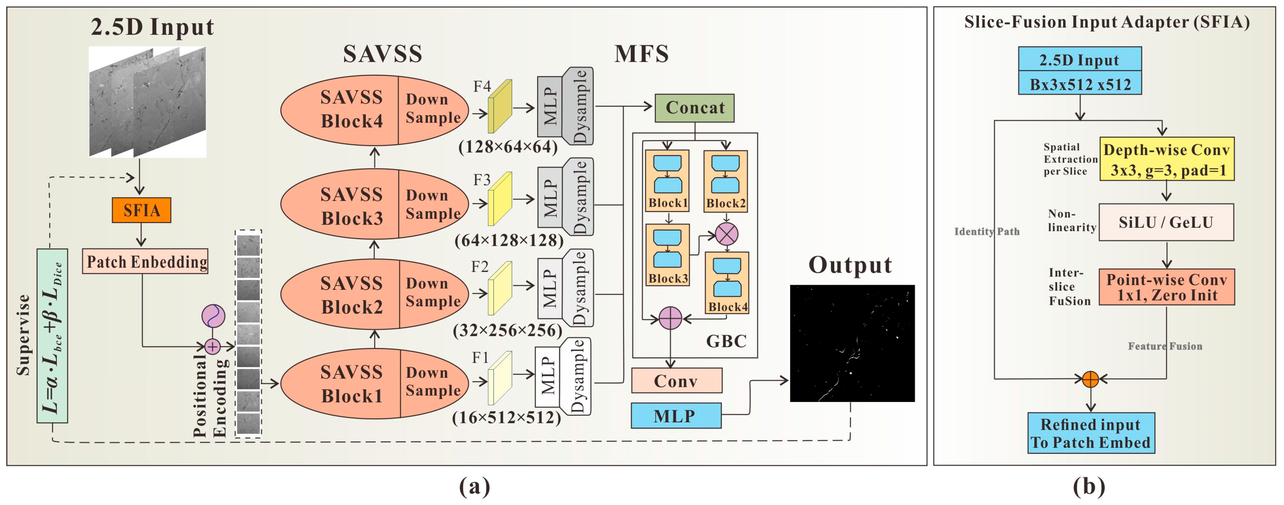
As shown in Figure 3a, the 2.5D SCSegamba framework adopts a four-stage encoder–decoder architecture. The input pore images are cropped to 512 × 512 and then processed by the Slice-Fusion Input Adapter (SFIA) module to capture 2.5D inter-slice pore continuity, followed by the SAVSS module for texture and morphological feature extraction. The encoder progressively downsamples spatial resolution while increasing the channel width, producing multiscale feature maps. These features are then upsampled to the original resolution and concatenated in the mmultiscalefeature segmentation (MFS) module, and a lightweight prediction head finally generates pixel-wise binary segmentation maps.
To address the channel adaptability issue, retain the pre-trained feature extraction capability of the original SCSegamba backbone, and enable pore connectivity validation across adjacent FIB-SEM slices; this study proposes a 2.5D slice-stacking strategy and an SFIA module.
2.5D Input Construction: Specifically, in the training stage, this study stacks the target slice with its upper and lower adjacent slices to form a three-channel tensor. For the first and last slices where an adjacent neighbor is missing, this study replicates the target slice to complete the three-channel tensor. The ground truth corresponds exclusively to the mask of the central slice. During the validation and testing stage, the input is constructed by triplicating the target slice.
SFIA is inserted before the Patch Embedding layer to explicitly encode cross-slice cues at the input stage. As illustrated in Figure 3b, its architectural design and optimization strategy are summarized as follows.
Decoupled spatial extraction and slice fusion: SFIA processes the input slices X i n R B × 3 × H × W in two stages. First, a depth-wise 3   ×   3 convolution (groups = 3) filters each slice channel independently, preserving slice-specific morphological details without cross-channel interference. Next, a SiLU activation [57] is applied, followed by a point-wise 1 × 1 convolution that aggregates features across the channel dimension, explicitly fusing information from the three slices to enhance inter-slice contextual cues for subsequent segmentation. All convolutions use stride 1; the depth-wise convolution uses padding 1, thereby preserving the spatial resolution.
Zero-initialization [58] and Residual Learning [59]: This study employs a residual formulation X o u t = X i n + F ( X i n ) . Crucially, the weights of the final point-wise convolution are initialized to zero (with bias disabled or set to zero), so that, at the start of training, F ( X i n ) = 0 and X o u t = X i n . This design stabilizes fine-tuning by ensuring that the backbone initially receives unmodified inputs, while allowing the model to progressively learn 2.5D inter-slice consistency cues.
The overall workflow comprises three main phases: (1) data preprocessing and dataset partitioning; (2) on-the-fly data augmentation; (3) end-to-end model training.
This study applied a standardized preprocessing pipeline. First, rigid registration was performed on the FIB-SEM images within the same specimen block. Second, the images were cropped to a consistent region of interest (ROI) to remove invalid margins and acquisition-related borders. Stripe artifacts were then removed using Wavelet–Fourier Filtering (WFF). Next, percentile clipping was applied to intensity values to mitigate the impact of outliers. Finally, normalization was performed to map image intensities uniformly to the [0, 1] interval, eliminating variations in imaging brightness and significantly accelerating model convergence.
Experimental observations indicate that adjacent FIB–SEM slices exhibit high similarity. As a result, conventional random dataset splitting may place near-identical images into the training, validation, and test sets, leading to an inflated estimate of model performance. Consequently, the dataset was split based on specimen blocks (or distinct depth intervals) to avoid any data leakage between the subsets. A dataset of 2000 images was constructed from 8000 FIB–SEM slices acquired from four specimens. Manual annotations were produced using the Computer Vision Annotation Tool (CVAT). The dataset was then split into training, validation, and test sets at a 7:1:2 ratio (training/validation/test = 1400/200/400 images).
Adopting the philosophy of the nnU-Net [60], this study employed on-the-fly data augmentation during training. In the experiments, this study observed that scaling and elastic deformation augmentations could cause narrow and elongated pores to vanish in the corresponding labels, thereby reducing the detectability of fine-scale structures. Therefore, this study only applied spatial augmentations such as random rotations and mirror flipping, while intensity transformations and low-resolution simulations were enabled using standard settings.
The training data flow is described as follows. An input tensor in R B × 3 × 512 × 512 is first processed by the SFIA module without changing the spatial resolution and is subsequently projected by the Patch Embedding layer into a feature map of size ( B × 16 × 512 × 512 ). This feature map traverses the first SAVSS Block at the original resolution before undergoing downsampling to B × 32 × 256 × 256 , effectively halving the spatial resolution while doubling the channel depth; This procedure is repeated through three additional SAVSS blocks and their corresponding downsampling operations, yielding a final encoder output of B × 128 × 64 × 64 and completing the encoder’s multiscale representation learning. The four stage-wise feature maps are then delivered to the Multiscale Feature Segmentation head (MFS), which dynamically upsamples and aligns them to a common resolution; they are concatenated along the channel dimension to form a fused tensor of B × 240 × 512 × 512 . The fused features are further processed by the GBC module and a 1 × 1 convolution to produce the final pixel-wise segmentation probability map (Pred) of B × 1 × 512 × 512 . In this study, with the batch size B set to 32, the network weights are updated via backpropagation by calculating the loss L against the corresponding Ground Truth (GT) masks B × 1 × 512 × 512 . To mitigate pixel-level class imbalance between the shale matrix and pore regions, this study utilizes the SCSegamba compound loss, defined as a weighted combination of Dice Loss [61] and Binary Cross-Entropy (BCE) loss [62]:
L = α·LDice(Pred,GT) + β·LBCE(Pred,GT).
Unlike SCSegamba, this study sets the ratio of α to β to 1:1.
This study built a network on an AMD Ryzen Threadripper 7960X CPU and two NVIDIA GeForce RTX 5090 GPUs (32 GB each), using Python 3.9 and PyTorch v1.13.1. During training, the patch size was set to 512 × 512 with a batch size of 32. This study used AdamW as the optimizer with a learning rate of 0.0005 and a weight decay of 0.01. The learning rate was scheduled using PolyLR with power = 0.9. The training process was run for a maximum of 300 epochs with early stopping enabled. During inference, a sliding-window strategy was adopted with a tile size of 512, an overlap ratio of 0.5, and a stride of 256.

3.6. Reconstruction of 3D Pore Surface Point Cloud

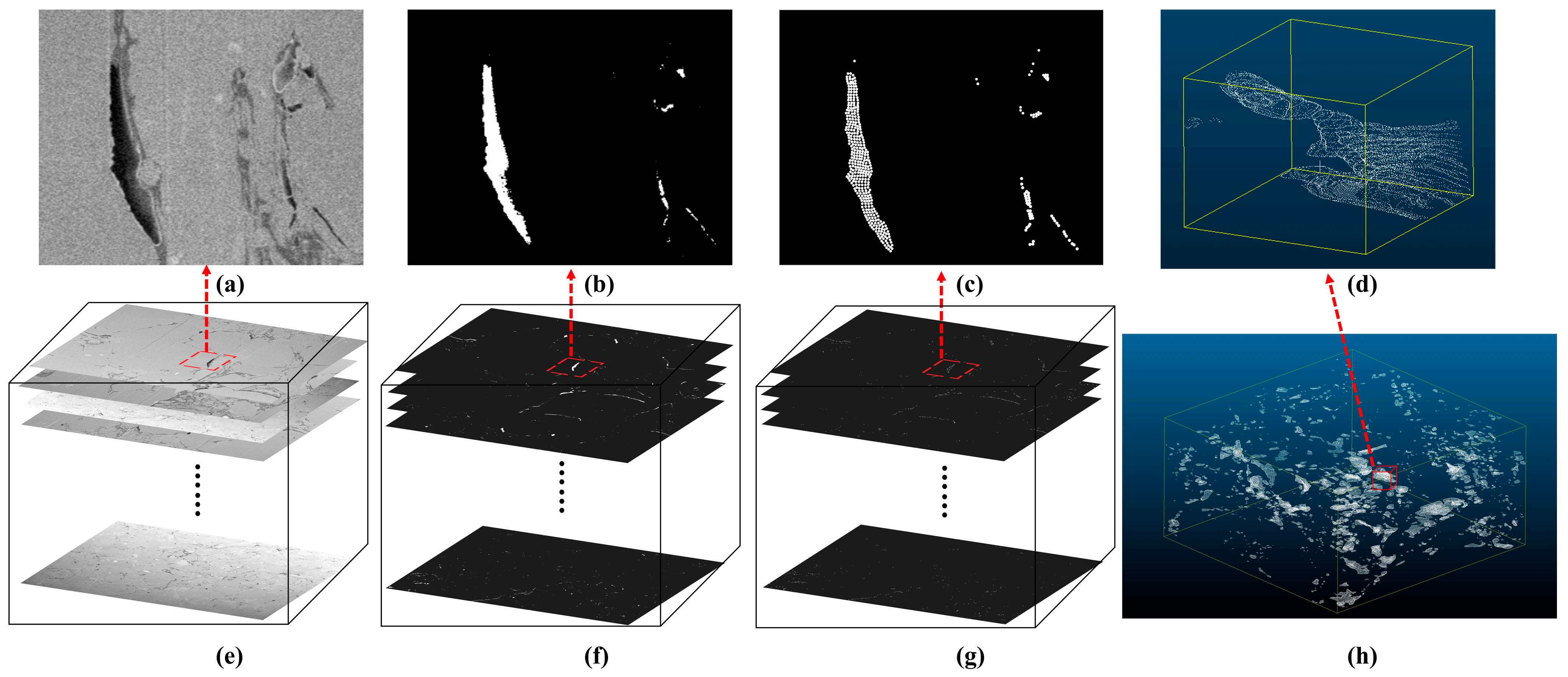
In this study, the high-quality pore segmentation results derived from FIB-SEM slices are treated as discrete point sets. After slice-wise alignment, these point sets are mapped into a unified 3D coordinate system, and a neighborhood-based boundary identification algorithm is applied to extract surface points and construct a 3D pore surface point cloud. Performing 3D analysis directly on the point cloud maximizes the preservation of pore information in its original form.
The detailed workflow illustrated in Figure 4 is described as follows. Based on the pore segmentation results, a binary pore indicator I z ( x , y ) { 0,1 } is first obtained for each slice, where 1 denotes pore space and 0 denotes the solid matrix. To avoid incomplete 3D interface information caused by retaining only 2D outlines, this study preserves all discrete points within the 2D pore interior and stacks them along the slice direction to construct a 3D pore-occupancy function:
V(x,y,z) = Iz(x,y), (x,y,z) ∈ Ω,
where Ω denotes the 3D data domain. The data size in this study is 1001 × 1001 × 501. A critical challenge in 3D FIB-SEM analysis is the anisotropy of the acquired voxels, where the in-plane resolution (10 nm × 10 nm) differs from the slicing step size (15 nm). Applying standard 3D box-counting directly to slice index coordinates would result in physically rectangular boxes, distorting the morphological complexity. To strictly correct for this anisotropy, this study established a unified 3D physical coordinate system where 1 spatial unit corresponds exactly to 10 nm. Here, x and y are the discrete in-plane coordinates of the 2D segmentation (i.e., point coordinates in the slice coordinate system), and z denotes the slice coordinate (1.5 times the slice index) along the stacking direction. Thus, the point cloud coordinates take both integer and half-integer values along the z-axis (e.g., 0, 1.5, 3.0, 4.5, …). This rigorous transformation ensures that the reconstructed point cloud is isotropic in the morphological space, providing an unbiased physical foundation for subsequent fractal analyses.
Within the 3D domain, the pore–matrix interface point set is determined using a discrete neighborhood relationship. Let N 6 = { ( ± 1,0 , 0 ) , ( 0 , ± 1,0 ) , ( 0,0 , ± 1 ) } denote the set of 6-neighborhood offsets. A point (x,y,z) (x,y,z) (x,y,z) is identified as an interface point if and only if it belongs to the pore phase and at least one of its 6-neighbors belongs to the matrix phase, i.e.,
S(x,y,z) = 1⟺V(x,y,z) = 1 ∧ ∃δ ∈ N6, V(x + δx,y + δy,z + δz) = 0.
Accordingly, the pore surface point set is obtained as
ΩS = {(x,y,z)∣S(x,y,z)} = 1.
The 6-neighborhood criterion was adopted over 18- or 26-neighborhood alternatives to strictly define the surface point set. In discrete topology, 18- or 26-connectivity includes points that contact the matrix only via edges or corners. Including these diagonal neighbors would generate a ‘thickened’ point cloud with redundant points that are geometrically offset from the primary interface, potentially biasing micro-roughness and surface fractal estimation. By restricting the definition to 6-connectivity, this study ensures that the extracted point cloud represents the geometrically minimal surface layer, thereby maximizing the fidelity of the subsequent fractal analysis.
The spatial coordinates of points in Ω S are then taken as the 3D pore surface point cloud for fractal dimension estimation. In this study, coordinate axis consistency is maintained, and discrete units are used for scale setting and fitting.
In parallel, 3D reconstruction was performed using the conventional serial-section reconstruction algorithm and Marching Cubes algorithm [63], followed by quantitative analysis of pore structure. However, subsequent experiments indicated that the interpolation, resampling, and smoothing steps inherent to this process introduce hard-to-quantify artifacts. These artifacts affect the accuracy of the 3D fractal analysis. These experiments are presented and discussed in Section 5.2.

3.7. Fractal Dimension Analysis of 3D Pore Surface Point Cloud

The fractal dimension of the pore surface point cloud Ω S is computed using the 3D box-counting method [64]. For a given box size ε, cubic boxes with side length ε are used to cover the point set, and the number of non-empty boxes N ( ε ) (i.e., boxes containing at least one surface point) is counted. In theory, if the point set exhibits fractal scaling over a certain range of ε, it follows a power-law relationship: N ( ε ) ε D , which yields, after taking logarithms,
lnN(ε) = Dln(1/ε) + C,
where D is the box-counting fractal dimension and C is a constant. To eliminate subjective bias in selecting the linear scaling range, this study established a strict mathematical sequence for box scale selection. The box sizes (ε) were restricted to a predefined physical window ranging from 2 to 64 units (corresponding to 20 nm to 640 nm). The lower bound ε m i n = 2 is selected to reduce voxel-grid discretization effects that can dominate at the single-voxel limit, whereas the upper bound ε m a x = 64 (approximately one-eighth of the shortest side, 501) is chosen to mitigate finite-size and boundary effects while maintaining sufficient box counts for stable regression. To achieve a dense, logarithmically uniform sampling without arbitrarily picking data points, the discrete box sizes were generated using a geometric progression with a constant ratio of r = 1.5. Each box size was calculated as a function of the scaling step n and rounded to the nearest integer, mathematically defined as εn = round (2 × 1.5n). This predefined criterion yielded an objective sequence (2, 3, 5, 7, 10, 15, 23, 34, 51). The fractal dimension D is then estimated by performing linear regression on the selected scale sequence in the lnN(ε) versus ln(1/ε) space. The goodness of fit (R2) is reported to objectively quantify scaling linearity. The slope of the regression line is taken as the estimated fractal dimension:
D = d (lnN(ε))/d (ln(1/ε)).
Furthermore, to mitigate the periodic step effects caused by the z-axis sampling sparsity with slice thickness (i.e., sampling anisotropy) and to robustly incorporate ε = 2 in our regression, this study integrated an 8-offset translation-averaging algorithm. For each box size ε, rather than computing the box count from a single default origin, the grid is shifted by ε/2 along the x-, y-, and z-axes, generating 8 symmetric coordinate offsets. The final box count N(ε) is determined by averaging the results from these 8 independent grid placements. These combined measures neutralize grid-origin bias and aliasing artifacts, ensuring a highly robust and geometrically accurate estimation of the 3D fractal dimension.

4. Results

4.1. Geochemical and Mineralogical Characteristics

Bulk geochemical and mineralogical datasets for the Kong 2 shale samples are summarized in Table S1, together with semi-quantitative XRD mineral abundances. Overall, the Kong 2 interval is mineralogically dominated by a mixed assemblage of felsic minerals (quartz + feldspar) and carbonate minerals, with subordinate clay minerals, analcime, and minor pyrite and siderite. Quartz contents range from 4.0 to 39.0 wt% (average 15.2 wt%), whereas feldspar varies between 4.0 and 59.0 wt% (average 24.0 wt%). Dolomite displays the broadest variability (0.0–64.0 wt%, average 26.2 wt%), reflecting pronounced compositional heterogeneity within Kong 2. Analcime is also highly variable, with an average abundance of 5.7 wt%, while clay minerals range from 5.0 to 42.0 wt% (average 18.1 wt%). In the ternary space defined by calcareous minerals, clay minerals, and siliceous minerals, the samples exhibit a wide compositional spread, indicating substantial mineralogical variability across the studied interval. Samples plotting close to the felsic-rich corner are characterized by high quartz + feldspar contents and were classified as siliceous shale, whereas samples located toward the carbonate-rich corner were assigned to calcareous shale (Figure S1). Clay minerals are generally subordinate in the Kong 2 interval, and most samples do not show very high clay contents. To distinguish the subset with relatively elevated clay contents and their transitional mineral compositions, this study defined a third group as clay-enriched mixed shale, using clay minerals > 20 wt% as the classification threshold. This cutoff is intended to capture samples with higher clay proportions than the bulk of the dataset, even though the overall clay content of the study interval is moderate. The threefold scheme (siliceous shale, calcareous shale, and clay-enriched mixed shale) provides a consistent mineralogical framework for comparing pore structure attributes among rock types in the following sections.
The Kong 2 shales are generally organic-rich. TOC values range from 0.3 to 11.3 wt% (average 3.2 wt%), and over half of the samples exhibit TOC contents exceeding 2.0 wt%. Rock-Eval parameters show S1 = 0.2–9.4 mg HC/g rock (average 2.6 mg/g) and S2 = 0.13–128.4 mg HC/g rock (average 20.9 mg/g). The combined generative potential (S1 + S2) spans 0.3–134.4 mg HC/g rock (average 23.6 mg/g). On the S2–TOC cross-plot (Figure S2), the Kong 2 samples mainly fall within the good to excellent source potential fields [65], consistent with strong hydrocarbon generative capacity. Hydrogen index (HI) values are relatively high, ranging from 44.4 to 1136.8 mg HC/g TOC, suggesting predominately oil-prone organic matter in much of the dataset. In the HI-Tmax diagram (Figure S3), most data cluster over a relatively narrow Tmax interval, and plot predominantly within the Type II to Type I–II kerogen fields, consistent with largely oil-prone organic matter [66]. The data distribution relative to the Ro = 0.5% and Ro = 1.0% reference curves suggests that the studied Kong 2 shales are mainly in the low to moderate maturity range.

4.2. Qualitative Pore Type and Morphological Characteristics

The Kong 2 shales exhibit diverse pore space types across micro- to nano-scales. Fractures are recognized from both core-scale observations and microscopy. Argon-ion polishing coupled with scanning electron microscopy (SEM) indicates that pore space in the Kong 2 samples can be broadly grouped into inorganic pores, organic matter (OM) pores, and microfractures.
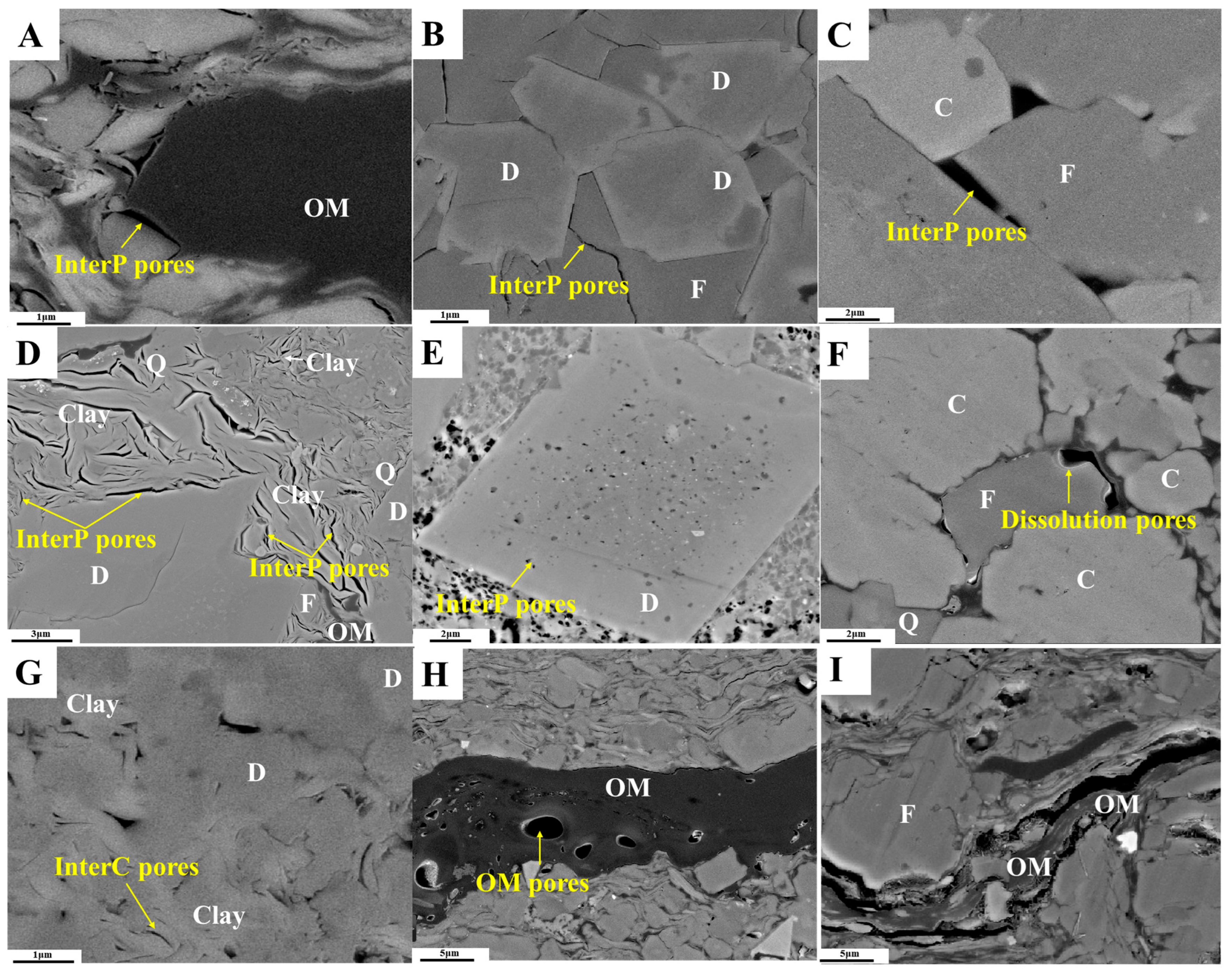
Inorganic pores are further classified, based on their spatial relationship to mineral grains, into interparticle, intraparticle, and intercrystalline pores. Interparticle pores are the most prevalent and volumetrically important type. They display variable geometries, commonly triangular, polygonal, or slit-like, with relatively smooth and straight pore walls. Interparticle pores occur (1) along organic–inorganic interfaces (Figure 5A), (2) at grain boundaries among feldspar, quartz, clay minerals, and other detrital grains (Figure 5B), (3) within pressure shadows adjacent to rigid grains (e.g., quartz, feldspar, and bioclasts) (Figure 5C), and (4) between platy clay aggregates where abundant slit-shaped pores are developed (Figure 5D).
Intraparticle pores are primarily related to mineral dissolution and occur within or along the margins of susceptible grains, including feldspar and carbonate dissolution pores (Figure 5E). These pores are typically small, with rounded to elliptical outlines, and may also occur along grain surfaces and edges (Figure 5F). Intercrystalline pores are mainly associated with clay minerals and dolomite, where spaces between adjacent crystals provide localized nanoscale storage and may form limited micro- to nano-scale transport pathways when interconnected (Figure 5G).
The occurrence of OM-hosted pores is influenced by OM abundance and composition, as well as the presence of solid bitumen. In the studied samples, OM pores are locally discernible (Figure 5H) but are predominantly nanoscale, suggesting a limited contribution to effective storage and flow at the imaging scale. OM-related shrinkage microfractures are occasionally observed, typically developing along clay–OM interfaces. These microfractures typically range from 5 to 10 μm in length (Figure 5I) and may locally enhance connectivity between adjacent inorganic pore domains.

4.3. Quantitative Pore Structure Characterization

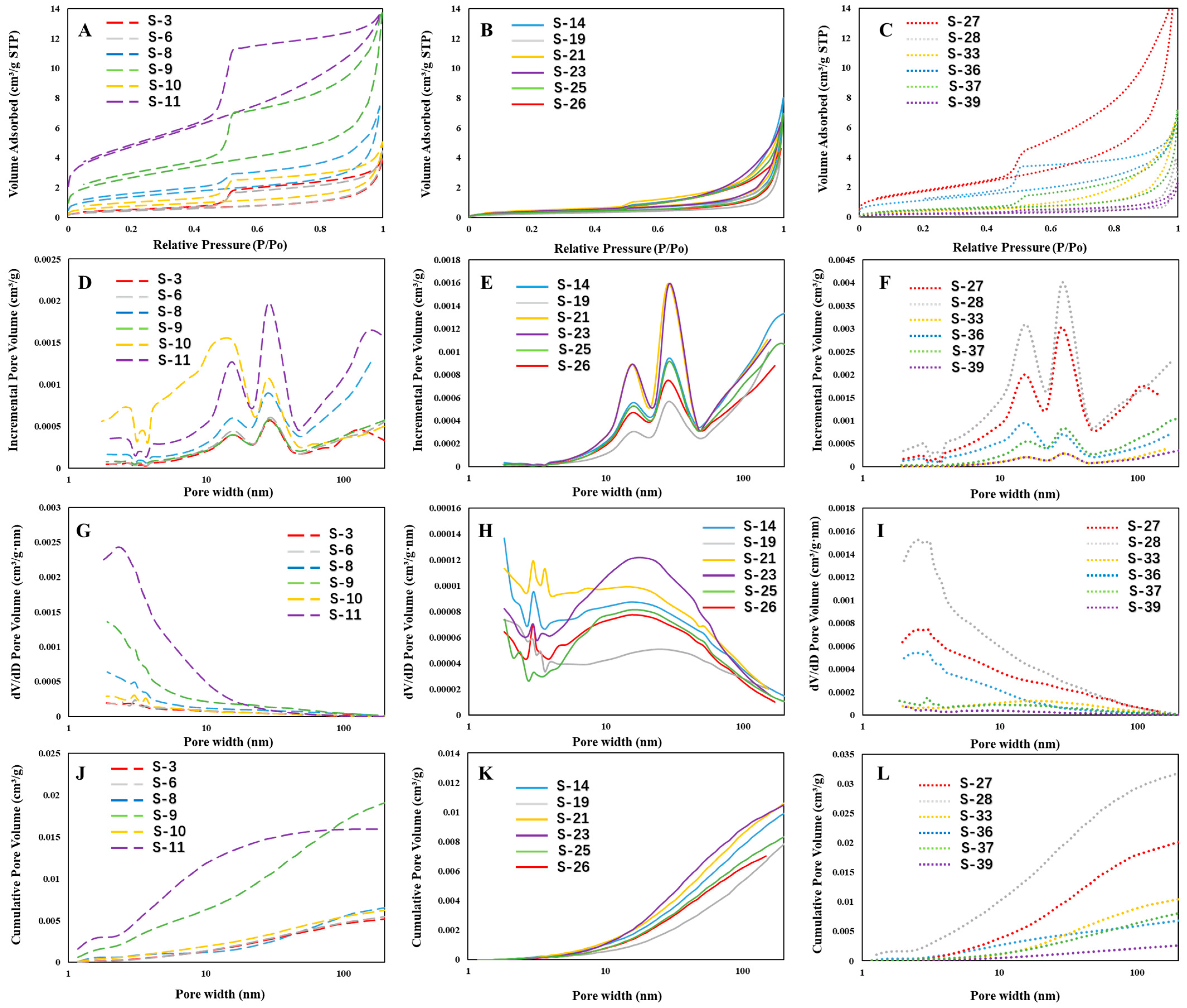
LPNA is widely used to characterize nano- to meso-scale pore systems in organic-rich shales, with an effective pore size window ranging from 0.35 to 200 nm [50,51]. In general, the adsorbed N2 volume reflects the amount of adsorption-accessible pore space and provides indirect information on pore network complexity. In this study, pore sizes are discussed using the IUPAC terminology, in which pores are classified as micropores (<2 nm), mesopores (2–50 nm), and macropores (>50 nm). In addition, the shapes of adsorption–desorption hysteresis loops were interpreted using the H1–H4 scheme summarized by Sing [67] based on the de Boer classification. The Kong 2 shale samples display type IV isotherms with pronounced hysteresis, indicating that mesopores contribute substantially to the adsorption-accessible pore system (Figure 6). Notably, the hysteresis characteristics vary among the three rock types. The clay-enriched mixed shales (Figure 6A) generally exhibit H2-dominated hysteresis, manifested by a marked separation between adsorption and desorption branches and an evident step in the intermediate relative-pressure range, consistent with pore-blocking effects and ink bottle-type pore geometries. The siliceous shales (Figure 6B) show a comparatively narrower hysteresis loop approaching the H3 type, suggesting a larger contribution from slit-shaped pores associated with aggregated particle frameworks. The calcareous shales (Figure 6C) show more variable behavior, with mixed H3–H2 characteristics: most samples resemble H3-type hysteresis, whereas several display clearer H2-like features.
Quantitatively, SSA was calculated using the BET method, and pore volume was derived from the N2 isotherms. The Kong 2 samples yield SSA values of 0.41–16.93 m2/g (mean 3.48 m2/g) and total pore volumes of 0.0026–0.0307 cm3/g (mean 0.0161 cm3/g). Rock-type comparisons reveal systematic differences. Siliceous shale has the lowest mean SSA (1.17 m2/g) and a pore volume of 0.0094 cm3/g, consistent with its relatively weak hysteresis and H3-like behavior. Calcareous shale shows intermediate values (mean SSA 3.65 m2/g; pore volume 0.0106 cm3/g) and predominantly H3-type hysteresis. Clay-enriched mixed shale exhibits the highest mean SSA (5.61 m2/g) with a pore volume of 0.0105 cm3/g, consistent with its more pronounced H2-type hysteresis and stronger pore structure heterogeneity. Across the three lithofacies, pore volume contributions are dominated by the mesopore range (2–50 nm). Siliceous shales exhibit the most focused and internally consistent pore size distributions, whereas the clay-rich shales show the broadest distributions and the strongest sample-to-sample variability. In contrast, the calcareous shales tend to display more pronounced mesopore peaks.
Fractal dimensions derived from the N2 isotherms provide additional constraints on pore structure heterogeneity and complexity. Fractal dimensions were calculated using Equation (1), and the corresponding regressions are illustrated in Figure 7. All fits show coefficients of determination R2 > 0.90. Two adsorption-derived fractal dimensions were obtained, denoted D1 and D2 (Table S2). D1 characterizes the low-relative-pressure regime (typically below ~0.47–0.50) and is commonly interpreted to reflect the fractal behavior associated with adsorption in very small pores, where adsorption is dominated by molecule–surface interactions. D2 corresponds to the medium-to-high-relative-pressure regime (typically above ~0.47–0.50) and reflects the geometric irregularity and heterogeneity of larger pores (mesopores to macropores) involved in multilayer adsorption and capillary condensation. To ensure the statistical reliability of the inter-facies comparisons, the uncertainties of the computed fractal dimensions were quantified. The standard errors (SEs) of the linear regressions are exceptionally low (Table S3); a window-sensitivity analysis, performed by perturbing the fitting bounds, demonstrated that the maximum absolute variations in the computed dimensions are highly constrained (Table S3). These narrow variation margins confirm that the observed differences in mean fractal dimensions among the various lithofacies represent genuine variations in pore structure complexity rather than overlapping statistical noise. Although fractal results derived from N2 adsorption represent the statistically averaged characteristics of the bulk shale sample, they effectively capture the intrinsic heterogeneity and roughness of the pore network. The results show that the clay-enriched mixed shale shows higher D1 values (average 2.51) than the siliceous shale (average 2.45) and the calcareous shale (average 2.45). For D2, the siliceous shale yields the lowest values (average 2.51), while the clay-enriched mixed shale shows the highest D2 (average 2.63) (Table S2; Figure 7).
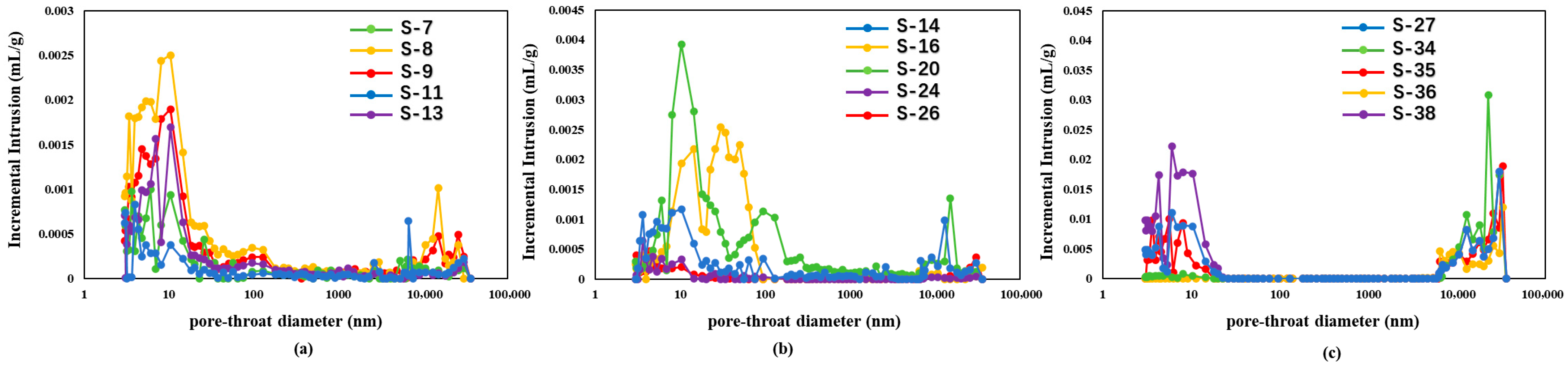
MIP was used to characterize pore-throat size distributions over a broader size window (3 nm–300 μm) than low-pressure N2 adsorption. The incremental intrusion distributions (Figure 8) indicate that pore-throat populations in the Kong 2 samples are concentrated in the meso- to macro-scale domain, with three prominent modes at approximately 3–20 nm, 50–200 nm, and 15–35 μm. Clear rock type differences are evident in both the position and magnitude of the fine-scale mode. The clay-enriched mixed shale exhibits its dominant nanoscale peak at approximately 10 nm (Figure 8a), whereas the corresponding peak for siliceous and calcareous shales shifts toward larger throat sizes (>10 nm) (Figure 8b,c). The siliceous shale generally exhibits a bimodal distribution comparable to the other lithofacies yet is characterized by a stronger contribution in the mesopore range, whereas the calcareous shale is distinguished by an additional macropore-scale peak near 10 μm (Figure 8). MIP-derived porosity ranges from 1.18% to 9.66% across the dataset. Mean porosities are 3.52% for the clay-enriched mixed shale and 5.02% and 6.70% for the calcareous shale and the siliceous shale, respectively. Similarly, the MIP-estimated permeability spans from 0.0069 to 0.030 mD. Consistent with the porosity trends, the clay-enriched mixed shale yields the lowest mean permeability (0.011 mD), followed by the calcareous shale (0.023 mD) and the siliceous shale (0.026 mD).

4.4. The Fractal Dimension of 3D Pore Surface

In this study, the box-counting method was employed to perform fractal analysis on the extracted 3D point cloud of the pore surfaces.
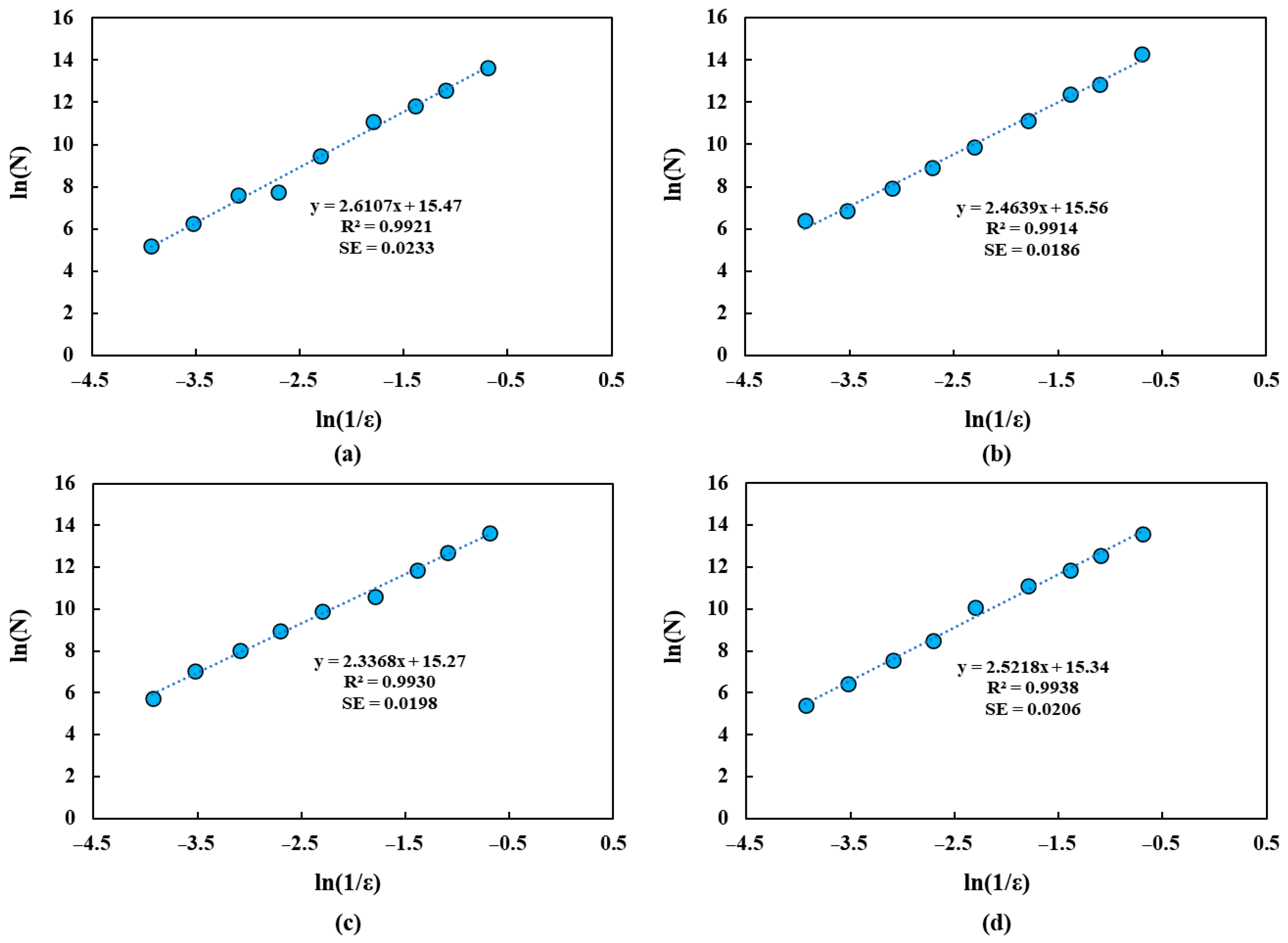
As shown in Figure 9, the box-counting results for the 3D pore surface point clouds of the four shale samples exhibit clear power-law scaling, with an approximately linear relationship between l n N ( ε ) and l n ( 1 / ε ) over the investigated predefined scale range ( ε ∈ [2, 51], corresponding to physical sizes from 20 nm to 510 nm). The linear fits yield consistently high coefficients of determination (R2 ≈ 0.991–0.994), indicating robust scale-invariant behavior of pore surface geometry at these scales. The fitted slope corresponds to the 3D pore surface fractal dimension D . The derived D slope values are 2.6107 (a), 2.4639 (b), 2.3368 (c), and 2.5218 (d), spanning 2.34 to 2.61. In addition to reporting the fitted 3D pore surface fractal dimensions, we quantify the statistical uncertainty of each estimate by the standard error (SE) of the regression slope. As annotated in Figure 9, the SE values for the four samples are 0.0233, 0.0186, 0.0198, and 0.0206, respectively, indicating that the slope estimates (i.e., D ) are well constrained over the selected scale range.

5. Discussion

The Kong 2 lacustrine shales in the Bohai Bay Basin represent a key shale oil reservoir interval, yet complex and heterogeneous pore systems remain a major challenge for reservoir characterization and quality prediction. Accordingly, the systematic, quantitative characterization of pore structure is essential for reliable reservoir quality assessment. This Discussion synthesizes pore structure results from SEM, N2 adsorption, and MIP, integrates fractal analyses derived from adsorption and FIB–SEM-based 3D pore surface characterization, and then evaluates the controlling factors and implications for reservoir quality.

5.1. Pore System Characteristics of Shale Reservoirs

Shales of the study area exhibit pronounced multiscale variability in pore structure, as reflected by systematic differences in pore morphology, pore size characteristics, SSA, and adsorption-derived fractal parameters. SEM observations provide direct constraints on pore types that effectively constitute the reservoir space, on pore morphologies, and on apparent 2D connectivity at the imaging scale. The resolvable effective pore volume is hosted predominantly by inorganic pore domains, which occur mainly as: (i) interparticle pores developed at grain contacts and organic–inorganic margins (Figure 5A–C); (ii) dissolution pores developed within or along the margins of soluble grains (e.g., feldspar and carbonate minerals) (Figure 5E,F); and (iii) intercrystalline pores within clay aggregates and locally within dolomite crystals (Figure 5G). Collectively, these inorganic pore domains comprise the principal pore structure elements discernible in SEM and therefore represent the most plausible contributors to pore space that appears more continuous at the submicron scale. In contrast, OM-hosted pores are only locally observed and typically appear as sparse nanometer-scale voids within OM patches. Their small size and discontinuous distribution in SEM images indicate that OM pores alone are unlikely to form a laterally extensive connected network in 2D (Figure 5H); instead, they more commonly occur as isolated or weakly connected nanoporosity embedded within an inorganic framework. Where present, OM mainly modifies pore boundary geometry at the interfaces between organic matter and minerals, rather than serving as a volumetrically dominant pore host. In addition to matrix pores, microfractures are intermittently observed and constitute an important structural component of the pore system. These features commonly develop along mechanically heterogeneous interfaces (particularly clay–OM contacts) and can link adjacent inorganic pore clusters that otherwise show limited 2D connectivity. Although volumetrically minor, such microfractures may locally improve pore continuity by linking adjacent pores and facilitating fluid migration across otherwise poorly connected matrix pores.
Integrating SEM observations (Figure 5) with LPNA (Figure 6) and MIP-derived (Figure 8) pore size distributions indicates that pore size characteristics are not uniformly coupled across samples. Although similar pore types are observed across samples, pore structure characteristics vary systematically among samples. Based on the IUPAC classification of hysteresis loops [67], the analyzed shale samples commonly display hysteresis behavior combining features of Types H2 and H3. The clay-rich mixed shale (Figure 6A) is dominated by an H2-type pattern, consistent with ink bottle-shaped pore geometry and pronounced pore-throat constriction, which can limit effective connectivity. In contrast, the siliceous shale mainly exhibits H3-type loops with a narrower hysteresis width (Figure 6B), indicating a substantial contribution from slit-shaped pores associated with rigid particle aggregates; such pore systems typically feature less severe throat restriction and more open transport pathways [67,68]. The calcareous shale (Figure 6C) displays mixed behavior: while most samples resemble an H3-type profile, a subset exhibits more distinct H2 features, suggesting the coexistence of slit-shaped and ink bottle-like pores with intermediate connectivity. It should be noted that pore shapes inferred from hysteresis loops are idealized interpretations, and natural shale pore systems typically comprise heterogeneous mixtures of pore morphologies. Cumulative pore volume versus pore width curves further indicate contrasting volume partitioning among lithofacies: pores toward the upper end of the measured range contribute significantly to total pore volume in the siliceous shale (Figure 6K), whereas micropores and mesopores dominate in the clay-rich mixed shale (Figure 6J). MIP extends this characterization to a broader throat-size spectrum, revealing multimodal distributions with prominent intervals at 3–20 nm, 50–200 nm, and 15–35 μm (Figure 8). Since MIP measurements are strongly influenced by pore-throat constrictions and are not directly comparable to LPNA-derived fractal descriptors, this study uses MIP primarily to constrain the pore-throat size distribution. The clay-rich mixed shale shows a dominant nanoscale mode centered at approximately 10 nm (Figure 8a), whereas the siliceous shale is shifted toward larger throat sizes, with the primary mode distributed between 10 and 100 nm (Figure 8b). The calcareous shale exhibits a pronounced micrometer-scale mode, consistent with the presence of microfractures and larger connected voids, alongside a secondary nanoscale mode between 5 and 20 nm (Figure 8c).
Consistent with these results, adsorption-derived fractal parameters further resolve the scale dependence of pore structure heterogeneity across the sample set. The low-pressure fractal dimension D1 varies between 2.36 and 2.69 and is derived from the low-relative-pressure segment, predominantly reflecting the surface roughness of adsorption-accessible micro- and mesopores. While D1 captures fine-scale surface asperities at the pore–solid interface, these smallest adsorption-accessible pore domains are not necessarily the primary source of lithofacies-scale differentiation in flow-related behavior, which is more strongly governed by pore network accessibility and constrictions in the larger pore system. By contrast, D2 is derived from the medium-to-high-relative-pressure regime associated with multilayer adsorption and capillary condensation, where hysteresis behavior and pore blocking are most diagnostic. Therefore, in the following analyses we use D2 as the main adsorption-derived fractal descriptor to evaluate lithofacies-dependent differences in mesopore-scale geometric irregularity and network non-uniformity. From a shale oil reservoir perspective, the multiscale pore attributes described above govern both hydrocarbon storage and hydrocarbon deliverability. Storage is contributed by the pore volume partitioning across micro–mesopores and by the development of adsorption-accessible surface area, which favors capillary retention and surface-associated hydrocarbons. Deliverability, in contrast, is primarily controlled by pore-throat effectiveness, bottleneck effects, and the degree to which mesopore domains are connected and can be linked by microfractures. Within this framework, D1 is interpreted mainly as a descriptor of the surface roughness of adsorption-accessible fine-pore surfaces; however, because fluid flow is principally governed by network accessibility/connectivity rather than fine-pore surface asperities alone, D1 is less directly indicative of inter-facies differences in reservoir deliverability than the larger, mesopore-to-macropore system. Consequently, D2 serves as a bulk indicator of mesopore-scale geometric irregularity and hysteresis-related network constraints. To translate these metrics into practical reservoir evaluation, higher D2 values tend to indicate a more irregular and throat-constrained mesopore network with stronger capillary condensation-related constraints, which is commonly associated with higher capillary resistance, stronger oil retention, and reduced transport efficiency. Conversely, lower D2 values suggest a more regular and accessible mesopore network with lower flow resistance, which is more favorable for liquid hydrocarbon mobility and for developing effective flow pathways following hydraulic fracturing.
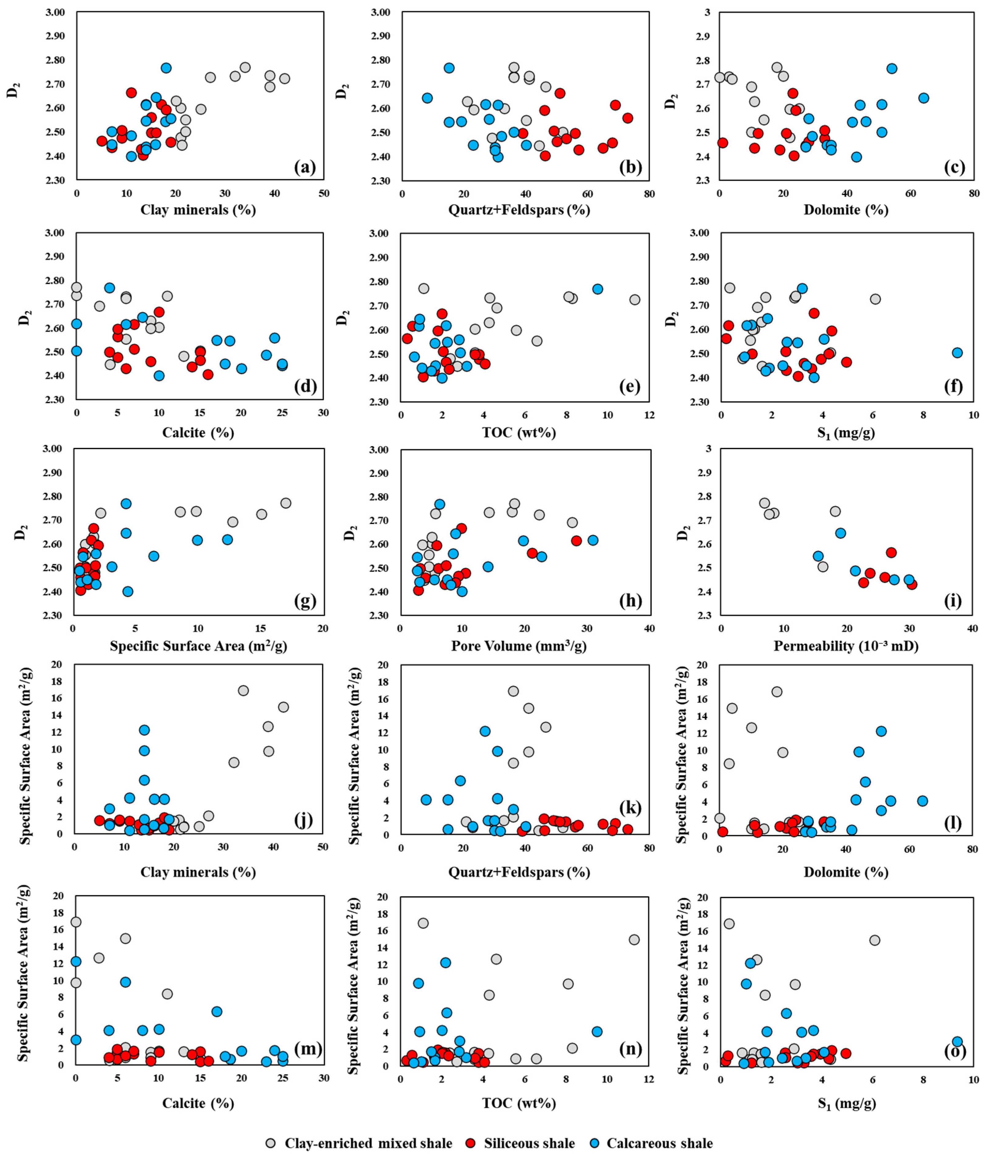
Building on the scale-dependent interpretation above, the bivariate cross-plots in Figure 10 indicate that D2 does not exhibit a unique dependence on any single compositional or geochemical variable. Instead, samples exhibit clustered, lithofacies-related patterns. This suggests that the heterogeneity signal captured by D2 reflects coupled, non-unique influences of mineral framework, microfabric, and pore network accessibility rather than a single dominant control. D2 generally increases with clay mineral content (Figure 10a), most clearly expressed in clay-enriched mixed shales. This tendency is consistent with the dominance of H2-type hysteresis and pore blocking signatures, and it is compatible with clay rich fabrics tending to develop narrow slit-like throats, tortuous pathways, and locally constricted pore connections. D2 decreases with increasing siliceous mineral content defined as quartz + feldspar, and this negative tendency is most clearly expressed in the siliceous shale samples (Figure 10b). This relationship suggests that a felsic-dominated framework may be associated with heterogeneity within the adsorption-accessible pore network, potentially reflecting a pore system with more regular slit-like interparticle geometries and a lower propensity for severe throat constriction and pore blocking. Alternatively, higher felsic fractions may correspond to more rigid grain-supported textures in which adsorption accessible pores are comparatively uniform, even where dissolution pores or local microfractures occur.
Carbonate phases show complex, non-uniform behaviors. The relationship between D2 and dolomite abundance displays a general V-shaped tendency (Figure 10c). Initially, D2 tends to decrease as dolomite content increases, reaching an apparent minimum at ~30%. At these low to moderate dolomite contents (<30%), dolomite-bearing fabrics and their associated diagenetic overprints may contribute to a stiffer framework and the preservation of relatively regular interparticle and intercrystalline pore geometries, thereby reducing the heterogeneity signal captured by D2. However, when dolomite abundance exceeds ~40%, D2 shows a clear increasing tendency with further increases in dolomite. In these highly dolomitized lithofacies (>40%), more pervasive dolomitization and related cementation and recrystallization may partially occlude pore space and enhance pore-throat constrictions and bottleneck effects, producing more irregular residual pore boundaries and stronger pore-blocking signatures. Such network constraints can elevate the geometric complexity recorded by the adsorption-derived D2. By contrast, within the relatively limited calcite range of the studied samples (generally ≤~30%), D2 exhibits an overall negative tendency with calcite abundance (Figure 10d). This behavior suggests that calcite in this concentration range does not pervasively fill and occlude the pore space. Instead, the localized presence of calcite, particularly where widespread calcite dissolution pores develop, may facilitate the preservation of relatively regular interparticle pore geometries, thereby suppressing irregularity within the adsorption-accessible pore network. Because higher calcite contents are not represented here, potential non-linear behavior at higher calcite fractions cannot be evaluated. Overall, these observations indicate that carbonate enrichment alone does not uniquely determine pore heterogeneity; rather, carbonate mineralogy, relative abundance, and associated diagenetic evolution jointly influence pore architecture and adsorption accessibility in the Kong 2 shales.
Organic variables show more dispersed relationships with D2. D2 displays an overall positive tendency with TOC (Figure 10e) but with substantial scatter, whereas the relationship with S1 is weaker and less systematic (Figure 10f). This pattern is consistent with SEM observations indicating that OM-hosted pores are locally present but are commonly nanoscale and discontinuous at the imaging scale. Accordingly, TOC is more likely to influence D2 indirectly through the interfaces of organic matter and minerals, bitumen distribution, and OM-related modification of pore boundary geometry, rather than through a simple volumetric increase in connected OM pore space. The broad scatter further indicates that organic matter alone does not provide a reliable predictor of heterogeneity within the adsorption-accessible pore network. In addition, D2 generally increases with SSA (Figure 10g), whereas its relationship with total pore volume is not consistently expressed (Figure 10h). This decoupling suggests that the heterogeneity signal captured by D2 is more closely linked to adsorption accessible surface development and mesopore-scale boundary irregularity than to bulk pore volume. Total pore volume can be disproportionately affected by a limited contribution from larger pores and fracture-like voids, which increase volume but do not necessarily dominate the adsorption-derived fractal response. In this sense, D2 behaves primarily as a measure of geometric complexity and accessibility within the adsorption-accessible pore network, rather than as a direct proxy for storage capacity. Importantly, D2 also shows an overall inverse tendency with MIP-estimated permeability (Figure 10i); samples with higher D2 generally exhibit lower permeability. This relationship supports the transport relevance of D2 in the sense that higher pore network heterogeneity is associated with stronger throat-controlled restriction and reduced effective transport capacity. Since the permeability is derived from MIP and primarily reflects pore-throat entry control, the D2–permeability relationship is used here as supporting evidence for transport relevance rather than as a universal permeability predictor. Notably, the pairwise correlations between D2 and individual compositional or geochemical variables are generally weak (Figure 10), indicating that D2 cannot be uniquely attributed to any single measured parameter. Instead, it serves as a valuable geometric indicator of pore network complexity, which provides important insights into fluid occurrence states and transport potential in lacustrine shale oil reservoirs.
Cross-plots of SSA against mineralogical and organic parameters indicate that SSA is most closely associated with clay mineral abundance (Figure 10j) and shows an overall inverse relation with felsic components (Figure 10k). Samples with higher clay mineral contents display markedly higher SSA, whereas higher quartz plus feldspar contents are generally associated with low SSA and a compressed range of values. Carbonate phases show contrasting behavior. SSA shows no systematic increase with calcite and tends to remain low at elevated calcite contents (Figure 10m), whereas dolomite-rich samples can retain moderate SSA but with substantial scatter (Figure 10l). Organic indicators show dispersed patterns. Relationships of SSA with TOC and S1 are weak and highly scattered (Figure 10n,o), suggesting that organic matter influences surface development mainly by modifying pore boundaries and by increasing surface complexity at interfaces between organic matter and minerals, rather than by simply adding organic hosted pores.
Overall, these results indicate pronounced multiscale variability in the pore structure of the Kong 2 shales and show that adsorption-derived fractal heterogeneity metrics reflect coupled compositional and textural effects rather than a single control. Because bulk responses and 2D observations provide limited constraints on pore geometry and its spatial organization, 3D pore geometry can offer more direct structural constraints and help reduce non-uniqueness in interpreting the inferred fractal behavior and its underlying controls.

5.2. 3D Pore Network Reconstruction, Visualization, and Fractal Analysis

This study performs point cloud-based 3D pore surface fractal analysis and conventional 3D reconstruction-based pore network visualization and quantitative characterization using FIB–SEM serial-section images. It should be noted that LPNA and MIP probe different effective sizes, whereas FIB–SEM provides image-resolved pore geometry within a localized volume. Considering the contrasting fractal responses of calcite-dominated and dolomite-dominated calcareous shales, representative samples from each type were selected. However, the accuracy of 3D reconstruction, as well as the subsequent topological and fractal analyses, relies fundamentally on the fidelity of the 2D image segmentation. Therefore, before interpreting the physical pore architectures, it is necessary to evaluate the reliability and potential biases of the segmentation algorithm.

5.2.1. Performance Evaluation and Bias Analysis of the Segmentation Models for FIB-SEM Slices

To evaluate the effectiveness of our 2.5D SCSegamba, this study benchmarked it against the original 2D SCSegamba and nnU-Net, with nnU-Net serving as a robust baseline for porous media image segmentation.
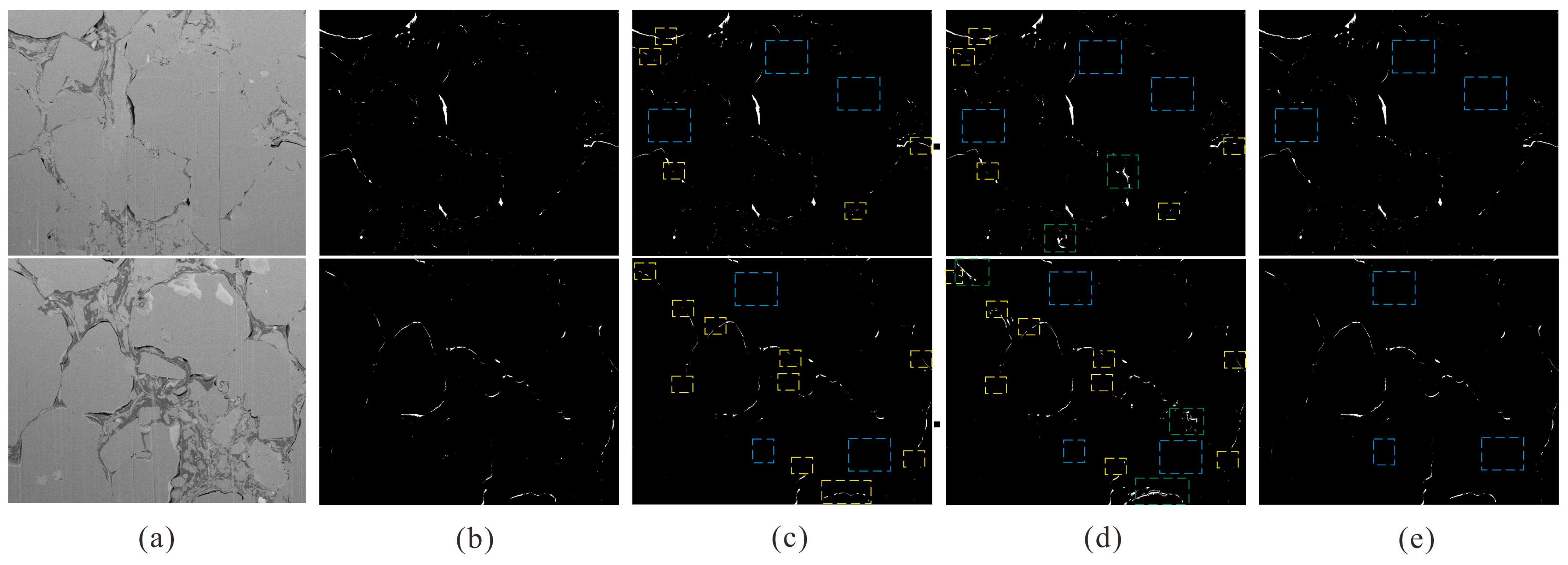
As illustrated in Figure 11, compared with the ground truth (b), the 3D nnU-Net result (c) fails to reliably capture narrow pore segments, often fragmenting elongated pore structures into discontinuous pieces. Moreover, isolated and spatially dispersed pores are frequently missed, indicating a limited sensitivity to fine-scale morphological features under strong class imbalance. In contrast, the original SCSegamba (d) better preserves elongated structures but introduces evident false positives by misclassifying the dark organic matter adjacent to pores as pore space; meanwhile, it still omits a non-negligible portion of isolated pores, in some cases even more severely than nnU-Net. Notably, the proposed 2.5D SCSegamba (e) achieves the closest visual agreement with the ground truth across both examples. It largely preserves the topological continuity of thin pore boundaries while substantially suppressing the organic matter-induced over-segmentation observed in (d), with remaining errors mainly confined to a few isolated pixels.
As shown in Table 1, four metrics were employed to assess the model performance: Recall (R), Precision (P), F1 Score (2RP/(R + P)) and mean Intersection over Union (mIoU). Precision and Recall measure the accuracy and completeness of the extraction results respectively. For binary pore segmentation, the F1 score was used to evaluate the balance between omission and commission errors of the pore class, whereas mIoU was used to measure the average overlap between predicted and ground-truth masks at the pixel level. All experiments were conducted on the dataset created in this study. For each model, this study selected the binarization threshold on the validation set by maximizing the F1 score. The selected threshold was then fixed and applied to the test set for all evaluations, with no threshold tuning on the test set. All models shared the same data split, threshold search range/step, and post-processing to ensure a fair comparison.
To perform a deep comparative analysis of the quantitative metrics, this study examines them in conjunction with the visual segmentation behaviors shown in Figure 11. The nnU-Net exhibited a relatively conservative prediction profile, achieving high precision (0.9113) but lower recall (0.8836), indicating limited false positives yet a substantial omissions of elongate structures; this imbalance is reflected in its F1 (0.8973) and mIoU (0.8921). Specifically, although it outperformed 2D SCSegamba in precision (0.9113 vs. 0.8802) and showed better qualitative retention of some isolated pores, the random scaling and elastic deformation employed in its data augmentation may distort extremely thin features, which can impair elongate pores detection and reduce overall foreground overlap. In contrast, 2D SCSegamba attained a slightly higher recall than nnU-Net (0.9016 vs. 0.8836) but noticeably lower precision (0.8802), consistent with its tendency to misclassify low-intensity organic matter as pores in the absence of inter-slice contextual constraints; consequently, its F1 (0.8898) and mIoU (0.8862) lagged behind nnU-Net despite the recall gain. Most notably, the proposed 2.5D SCSegamba delivered the best overall performance, demonstrating simultaneous improvements in recall (0.9301) and precision (0.9398) and achieving the highest F1 (0.9349) and mIoU (0.9241). This superiority supports its capacity to leverage inter-slice context effectively, preserving the continuity of thin, elongated pores while robustly suppressing false positives. It should be noted that the deep learning model utilized in this study was optimized for the specific lacustrine shale samples analyzed. Applying this framework to geological targets with significantly different lithologies or imaging conditions may require further fine-tuning to ensure optimal segmentation performance.
To explicitly quantify uncertainty propagation and assess the stability of the proposed point cloud-based 3D fractal estimates with respect to deep learning segmentation uncertainty, a sensitivity analysis was performed. Specifically, morphological erosion and dilation with a 1-pixel radius were applied to the segmented masks to simulate systematic under- and over-segmentation, respectively. Additionally, 0.5% of the pixels along the pore boundaries were randomly flipped to simulate stochastic segmentation artifacts. Each perturbed mask was subsequently subjected to the identical interface point cloud extraction and 3D box-counting workflow. As shown in Table 2, the point cloud-based fractal dimension (D) exhibits remarkable robustness to segmentation perturbations. As theoretically expected, morphological erosion slightly decreases D due to the smoothing of fine high-frequency asperities, whereas dilation and boundary noise inflate D by introducing artificial roughness. Importantly, the maximum relative change in D across all samples and perturbation settings remains below 0.8%. Even when accounting for potential misclassifications by the deep learning model at ultra-fine pore boundaries, the relative ranking of pore surface roughness among the different shale lithofacies (S-7 > S-36 > S-14 > S-35) remains entirely stable under all perturbation scenarios. Furthermore, this algorithm-induced uncertainty is significantly smaller than the intrinsic physical variations across the different lithofacies, confirming that the overall geological interpretations regarding pore system heterogeneity remain fundamentally unaffected.

5.2.2. 3D Visualization and Quantitative Analysis of Pore Networks via Traditional 3D Reconstruction

Using the validated 2.5D SCSegamba model, the FIB-SEM slices of the representative samples were precisely segmented. The segmented pore space was then reconstructed as a 3D voxel volume via conventional serial-section (slice-stacking) reconstruction, from which a 3D surface mesh was generated using the Marching Cubes algorithm, enabling 3D visualization and quantitative analyses of pore morphology, spatial distribution, and pore surface characteristics.
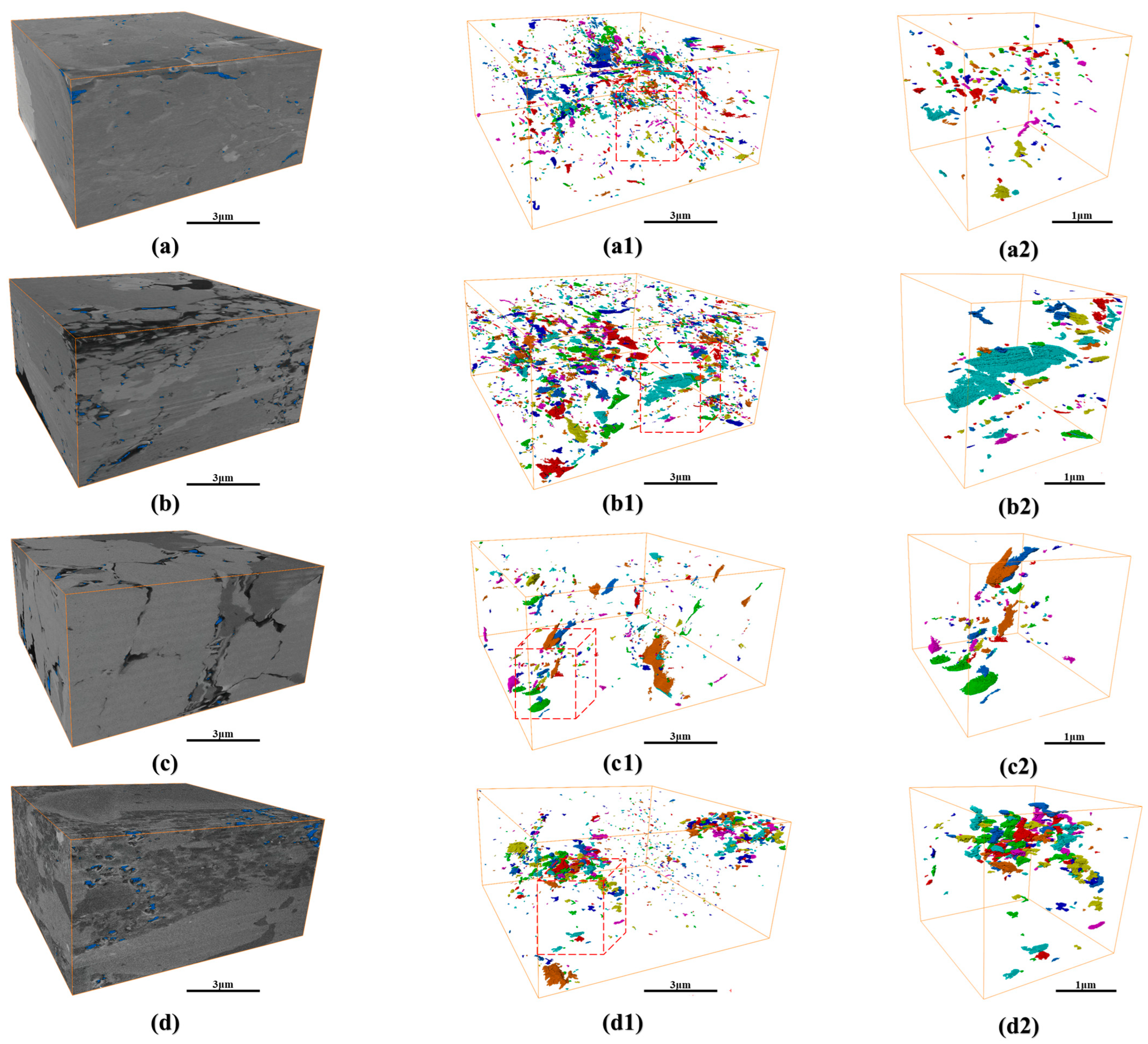
Across the four samples, the 3D reconstructions reveal the image-resolved pore space and the organization of connected pore components within the reconstructed volumes. In Figure 12(a1–d1), different colors denote distinct connected pore components, allowing a direct visualization of the organization and area of the connected pore space. The clay-enriched mixed shale contains an appreciable pore population, but pores occur mainly as discrete, small, connected components, and connectivity is readily interrupted (Figure 12(a1)), yielding a reconstructed porosity of 2.45%. By contrast, the siliceous shale displays more spatially continuous connected pore space (Figure 12(b1)). The enlarged view shows multiple interconnected pore regions with sharp and distinct pore boundaries, consistent with interparticle pores preferentially developed along the margins of rigid felsic grains and at grain contact zones (Figure 12(b2)). The siliceous shale also yields the highest porosity of 3.48%.
The calcite-dominated calcareous shale shows overall sparse pore occurrence and a low pore volume, yet the connected pore space includes several relatively large and well-connected pore regions (Figure 12(c1,c2)). These pores are predominantly sheet-like and preferentially developed along mineral grain margins, consistent with an interparticle origin, and they do not show pronounced signs of local pore blocking. This sample yields the lowest porosity of 1.80%. The dolomite-dominated calcareous shale contains a relatively abundant pore population and shows a clear dual connectivity pattern. One pore population is expressed as relatively large, connected pore regions that provide the main contribution to connected pore space and continuity within the reconstructed volume, as illustrated by the prominent connected regions in Figure 12(d1) and the enlarged view in Figure 12(d2). The second population consists of numerous small pores that occur as spatially dispersed and largely isolated features, contributing limited connectivity despite their abundance. This sample yields an image-resolved porosity of 2.39%. The coexistence of these two pore populations indicates a multiscale pore organization in which connected pore space is concentrated within a limited number of larger connected regions, while a background population of fine isolated pores is preserved throughout the volume. This architecture implies strong internal heterogeneity within the dolomite-dominated calcareous shale, with connectivity influenced by the distribution and linkage of the larger connected pore regions rather than by the overall abundance of small pores. Overall, the 3D reconstructions indicate systematic differences in how connected pore space is partitioned and organized among the four shale types, including distinct connectivity styles between the calcite-dominated and dolomite-dominated calcareous shales within the reconstructed volumes.
Pore diameters were quantified within the same 3D reconstruction framework using the equivalent diameter of individual segmented pores, and pore diameter probability distributions were compiled for each lithofacies, as shown in Figure 13. All four distributions are strongly right-skewed and are dominated by pores smaller than 200 nm, with a low probability extension toward larger diameters. The clay-enriched mixed shale is most strongly enriched in fine pores, showing a mode within the 30 to 50 nm interval and a gradual decrease toward larger diameters (Figure 13a). The siliceous shale is shifted toward larger pore diameters and displays a sharper mode centered around 50 to 70 nm, accompanied by a higher proportion of pores larger than 50 nm and larger than the other lithofacies (Figure 13b). The calcite-dominated calcareous shale, despite the lowest porosity, exhibits a comparatively coarse but relatively narrow distribution, with most pores concentrated between 50 and 100 nm and a limited contribution from the finest pores (Figure 13c). The dolomite-dominated calcareous shale shows the broadest pore size spectrum, combining a substantial fine pore fraction smaller than 50 nm with a more evident contribution from pores larger than 100 nm, including a sparse population extending beyond 200 nm (Figure 13d).

5.2.3. 3D Surface Fractal Analysis of Pore Networks

As discussed in Section 5.1, fractal dimensions were derived from N2 adsorption isotherms using the FHH model, and these metrics were used to discuss pore surface roughness and pore system heterogeneity of shales [69]. However, it is important to note that N2 adsorption captures a bulk, statistically integrated response of the whole sample rather than an accurate characterization of a specific region [15,70]. Furthermore, the hysteresis loops, particularly the desorption branch, are often influenced by pore network constraints rather than reflecting surface roughness alone [71]. Accordingly, this study applies the 3D box-counting method to FIB–SEM-derived pore surfaces to directly quantify fractal characteristics, thereby capturing the structural complexity of specific, spatially defined regions. In preliminary assessments, fractal dimensions computed from conventionally reconstructed surface meshes clustered within a narrow and unexpectedly low range across the four samples (e.g., 2.13 for the clay-enriched mixed shale (S-7), 2.05 for the siliceous shale (S-14), 2.06 for the dolomite-dominated calcareous shale (S-36), and 2.03 for the calcite-dominated calcareous shale (S-35), as shown under D (Traditional) in Table 2). This narrow spread and systematically low magnitude are inconsistent with the pronounced surface relief indicated by the FHH results and with typical ranges reported for shale pore surfaces. This discrepancy arises because surface-based fractal quantification is highly sensitive to the artifacts with which reconstructed pore boundaries are represented. Conventional 3D reconstruction workflows involve interpolation, resampling, and smoothing operations, which can modify small-scale surface undulations and may artificially regularize pore boundaries, thereby reducing apparent surface roughness. While such effects are often negligible for visualization and coarse-scale metrics, they can exert a disproportionately large impact on surface fractal analysis [72]. To minimize reconstruction-induced bias, this study performs fractal characterization of pore surface roughness directly on 3D pore surface point clouds constructed from the FIB-SEM segmentation results. Because this point cloud representation imposes no additional surface regularization, it preserves the original pore surface morphology to the greatest extent possible, thereby providing a more direct geometric basis for 3D surface fractal characterization.
It is also crucial to acknowledge that the box-counting surface fractal dimension derived from the FIB–SEM pore surface point clouds is inherently constrained by imaging resolution and the finite scaling domain that can be resolved. In this study, the pixel size was 10 nm in the x–y plane with a slice thickness of 15 nm, such that surface undulations below these sampling intervals cannot be captured and the lower cutoff of the scaling interval is instrument-limited. If the acquisition resolution were coarsened (larger pixel size and thicker slices), it would suppress high-frequency surface roughness in a manner analogous to low-pass filtering, potentially smoothing small-scale asperities and biasing D downward. Conversely, higher-resolution imaging could extend the accessible scaling range toward smaller ε and may yield higher or more stable D values if additional genuine roughness is resolved, until a physical lower cutoff is reached where fractal behavior no longer holds.
The 3D pore surface fractal dimensions differ among lithofacies and span a broad range, with values of 2.61 for the clay-enriched mixed shale, 2.46 for the siliceous shale, 2.52 for the dolomite-dominated calcareous shale, and 2.34 for the calcite-dominated calcareous shale (Figure 9; Table S4). Higher D indicates greater pore surface roughness and multiscale geometric complexity. Accordingly, these values collectively indicate pronounced multiscale roughness and non-Euclidean complexity of shale pore surfaces. Inter-sample differences in D further highlight heterogeneous pore surface organization. The clay-enriched mixed shale exhibits the highest value, consistent with a pore system dominated by fine pores and spatially fragmented connected pore space, where pore surfaces are more irregular. The dolomite-dominated calcareous shale also yields a relatively high value, consistent with the presence of both a relatively large, connected pore space and abundant small, spatially isolated pores within the reconstructed volume. The siliceous shale shows an intermediate value, consistent with connected pore space that is more spatially continuous and characterized by sheet-like interparticle pores developed along felsic grain margins with sharp, well-delineated pore boundaries. The calcite-dominated calcareous shale yields the lowest value, suggesting a comparatively more regular surface expression within the reconstructed volume, consistent with sparse overall pore occurrence but locally well-connected sheet-like interparticle pores and limited development of dispersed pores. Together, these point cloud-based results indicate that lithofacies-dependent heterogeneity is expressed not only in pore size statistics and connectivity patterns but also in pore surface geometric complexity, providing a direct geometric basis for comparison with adsorption-derived fractal responses.
To explicitly link the 3D pore surface fractal dimension to flow-relevant connectivity, this study further quantified coordination number (CN) statistics from the FIB-SEM reconstructed pore networks (Table S4). The siliceous shale exhibits the highest overall connectivity, yielding a mean coordination number of 1.19 and the highest effectively connected fraction, with 29.58% of its pores forming potentially flow-effective connections (CN ≥ 2). In contrast, the clay-enriched mixed shale and dolomite-dominated calcareous shale are severely fragmented, and their networks are dominated by strictly isolated pores (CN = 0) that account for 72.83% and 77.76% of the pore bodies, respectively, leaving only about 4% effectively connected. The calcite-dominated calcareous shale shows intermediate connectivity, characterized by a mean coordination number of 0.63 and 13.89% of its pores forming effective connections. To evaluate the physical relevance of the 3D pore surface fractal dimension as a reservoir descriptor, this study compared it with fundamental petrophysical attributes, specifically, the FIB–SEM-reconstructed volumetric porosity and the MIP-estimated permeability (Figure S4; Table S4). Notably, D shows no clear monotonic relationship with porosity (Figure S4a). This decoupling suggests that static storage capacity is not uniquely tied to the geometric complexity and multiscale roughness of the pore–solid interface. For example, relatively higher-porosity lithofacies may be dominated by comparatively smooth, larger pores (yielding a lower D), whereas a lower-porosity matrix characterized by abundant small pores with irregular boundaries can exhibit a higher D. By contrast, from hydrocarbon transport perspective, D exhibits an overall inverse tendency with MIP-estimated permeability (Figure S4b). Although permeability does not depend solely on pore volume fraction and is strongly influenced by pore-throat restriction and connectivity emphasized by MIP, the increase in permeability is broadly consistent with the decrease in 3D pore surface fractal dimension (2.61 to 2.34). This trend supports the interpretation that smoother pore surfaces and geometrically simpler pore boundaries, typically accompanied by less severe throat constriction and lower tortuosity, are associated with more effective flow pathways at the pore-throat scale. In clay-rich shales, higher surface roughness and geometric complexity coincide with stronger pore-throat restriction and more tortuous pathways, which can increase flow resistance and lower permeability. By contrast, in grain-supported siliceous and calcite-rich samples, more regular pore boundaries and less restrictive pore-throat architectures tend to coincide with higher permeability. Given the limited number of reconstructed volumes and the fact that permeability is estimated from MIP, this study presents this D–permeability relationship as transport-relevant and indicative rather than as a universal predictive model.

5.3. Interpretation of Multiscale Pore Structure and Heterogeneity

5.3.1. Lithofacies Contrasts in Multiscale Pore Characteristics

Multiscale pore characteristics across lithofacies in the Kong 2 shales were systematically evaluated by integrating LPNA, MIP, and FIB-SEM with fractal analysis, augmented by deep learning-based 2D pore segmentation and subsequent 3D point cloud reconstruction. This integrated workflow enables a consistent cross-scale characterization of pore types, morphologies, pore size distribution, and quantitative descriptors of pore surface complexity. LPNA provides constraints on adsorption-accessible pore volume, SSA, adsorption-derived fractal parameters, and nanopore size distributions. MIP extends characterization to larger pore-throat scales by quantifying pressure-dependent mercury intrusion responses. It should be noted that MIP results in this study are used primarily to constrain pore-throat restriction and accessibility and connectivity at larger scales, rather than to infer true pore-body sizes or to be directly equated with LPNA-derived fractal descriptors. FIB–SEM reconstruction directly quantifies pore geometry within imaged volumes, including connected pore space, pore size statistics, and porosity, thereby offering a direct geometric benchmark for interpreting bulk-averaged parameters. Furthermore, point cloud-based analysis yields a 3D pore surface fractal dimension that explicitly quantifies surface roughness. Collectively, these datasets elucidate systematic variations in pore size distributions and pore space organization.
Clay-enriched mixed shale is characterized by pores concentrated mainly at diameters smaller than 100 nm, together with the highest SSA and the largest fractal dimension D2. SEM observations commonly show slit-shaped interparticle pores developed between platy clay aggregates, together with local intercrystalline pores associated with clay-rich aggregates, as illustrated in Figure 5D,G. At the imaging scale, larger pores forming clearly continuous pore space are not prominent. Consistent with these textural characteristics, nitrogen adsorption isotherms display predominantly H2-type hysteresis in Figure 6A, which is commonly associated with strongly constricted pore connections and pronounced pore size contrasts within the pore system. MIP measurements further support this interpretation by showing a dominant intrusion mode concentrated mainly within 5–50 nm in Figure 8a. Likewise, although FIB-SEM reconstruction yields a non-negligible porosity of 2.45%, the 3D pore size probability distribution is dominated by pores smaller than 50 nm, and connected pore space occurs mainly as spatially discrete, small-scale regions in Figure 12a and Figure 13a. Taken together, these observations indicate that the clay-enriched mixed shale hosts a micro- to mesopore-dominated pore system with high surface development and strong heterogeneity, reflected by its high fractal dimension and the discontinuous character of connected pore space.
Siliceous shale exhibits a distinctly different pore system expression, with relatively low SSA and the lowest adsorption-derived fractal dimension D2 among the lithofacies. SEM images commonly show interparticle pores along quartz and feldspar grain boundaries and at interfaces between minerals and organic matter, together with dissolution-related intraparticle pores associated with susceptible grains, as illustrated in Figure 5A–C. Consistent with these textures, N2 adsorption isotherms display a comparatively narrow hysteresis loop with H3-type characteristics in Figure 6B, indicating a more regular slit-like pore geometry and a weaker hysteresis response than the clay-enriched mixed shale. MIP results support this interpretation by showing that the dominant intrusion diameter is shifted toward larger values relative to the clay-enriched mixed shale, with most pore diameters concentrated within 10–200 nm, as shown in Figure 8b. FIB-SEM 3D reconstruction further demonstrates the highest porosity, reaching 3.48%, and the 3D pore size probability distribution is shifted toward larger diameters with an increased contribution from pores larger than 50 nm, as shown in Figure 12b and Figure 13b. Taken together, these observations indicate that the pore system of siliceous shale is supported by a rigid felsic framework and is characterized by relatively larger pores, more continuous connected pore space, and a weaker heterogeneity signal reflected by its low fractal dimension.
For carbonate-rich shales, carbonate dissolution, recrystallization, and cementation can selectively modify pore walls and pore throats, potentially smoothing surfaces, occluding small pores, or generating secondary dissolution porosity. SEM observations indicate that pore space is commonly associated with carbonate-related textures, including dissolution related intraparticle pores developed along carbonate grains and local intercrystalline pores within carbonate crystal aggregates. Typical examples include dissolution pores within dolomite grains in Figure 5E and dissolution pores along calcite grain margins in Figure 5F. In addition, MIP commonly extends the pore size signal into the micrometer range and, besides the peak around 10 nm, reveals an additional peak near 10 μm as shown in Figure 8c. This feature is consistent with the presence of microfractures and locally enlarged dissolution pores, which may contribute disproportionately to connected pore space even where total pore abundance is limited. Within the calcareous shale suite, calcite-dominated and dolomite-dominated samples display distinct multiscale characteristics. For calcite-dominated calcareous shale, FIB-SEM reconstruction yields the lowest porosity, whereas the 3D pore size probability distribution is shifted toward relatively larger diameters, with pore sizes mainly concentrated within 50–100 nm as shown in Figure 12c. This pattern suggests that pore space is contributed primarily by a limited number of larger pores, whereas the smallest pore fraction is less developed. By contrast, dolomite-dominated calcareous shale shows a broader pore size distribution across methods and a clearer multiscale expression. FIB-SEM reconstruction yields a higher porosity than the calcite-dominated samples and reveals the coexistence of relatively large, well-connected pore regions together with numerous small, isolated pores, as shown in Figure 12d and Figure 13d. Taken together, carbonate-rich samples indicate that carbonate mineralogy is not a simple proxy for pore system properties. Differences between calcite-dominated and dolomite-dominated textures are expressed not only in pore abundance but also in characteristic pore sizes and in the spatial arrangement of connected pore space.
Integrated results from LPNA, MIP, SEM, and FIB-SEM show clear lithofacies-dependent differences in pore size distributions, fractal characteristics, and the spatial organization of pore space in the Kong 2 shales. These differences are expressed consistently in both bulk measurements and image observations, indicating that pore system variability is closely linked to compositional and textural attributes of the shale.

5.3.2. Controls on Pore System Development

At the lithofacies scale, the mineral composition determines both the location and organization of the pore system. This includes identifying which minerals or boundaries host the pores, as well as defining the microscopic arrangement and geometry of the pore throats. In shales with high clay content, pores are primarily found within clay aggregates and along grain boundaries. These boundaries occur between adjacent clay particles or between clay and brittle grains, creating conditions that favor narrow and winding pore shapes. Such fabrics tend to generate an abundant adsorption-accessible surface area yet simultaneously promote strong throat control through locally constricted pore-throat linkages and pronounced “bottleneck” effects. Consequently, these clay-rich domains intrinsically drive higher surface roughness, which is faithfully captured by the surface fractal dimension. This framework explains why pore systems characterized by abundant small pores and high surface areas exhibit restricted throat connectivity and spatial compartmentalization in 3D images (Figure 12a and Figure 13a). In contrast, a felsic-dominated framework (quartz + feldspar) is more prone to develop grain-supported microfabrics in which pore domains are expressed preferentially in interparticle regions and along more rigid boundaries. Even without exceptionally high surface area, such grain-supported microfabrics are commonly associated with a shift toward larger adsorption-accessible pore sizes and more effective mercury intrusion, because pore-throat constriction and pore-blocking effects are typically less pronounced than in clay-rich fabrics. The facies-grouped trends in the adsorption-derived heterogeneity signal are consistent with this interpretation: the mineral framework does not simply scale pore volume but governs the geometry and accessibility of the adsorption-accessible mesopore network.
The observed scatter between carbonate content and pore metrics (fractal dimension and SSA) suggests that carbonate abundance alone is insufficient to explain pore structure variability in carbonate-rich shales. The contrasting behaviors observed between calcite-dominated and dolomite-dominated calcareous shales suggest that carbonate mineral type can exert a meaningful influence on both pore preservation and pore modification pathways. Calcite is relatively reactive during diagenetic fluid–rock interaction and is prone to dissolution under acidic conditions, potentially generating secondary dissolution porosity [12]. Accordingly, in calcite-rich domains, dissolution followed by reprecipitation and recrystallization may alter pore bodies and throats; depending on the relative extent of dissolution versus cementation, porosity may be locally enhanced or partially reduced by pore filling. In contrast, dolomite-bearing fabrics may more readily retain microtextural heterogeneity and can experience phase-specific diagenetic overprints (e.g., cementation and recrystallization) that modify pore boundary roughness and pore-throat geometry. Such effects can broaden the range of adsorption-accessible pore sizes and be consistent with an enhanced heterogeneity signal captured by adsorption-derived metrics. Crucially, the resulting spatial complexity of the pore network is robustly reflected by the structural fractal dimension (D2 and D). Therefore, even lithofacies with broadly comparable carbonate richness may display markedly different pore size distributions and pore-throat effectiveness, depending on whether calcite or dolomite dominates within the load-bearing framework and the pore-hosting domains.
Although the HI spans a wide range (Figure S3), most samples plot predominantly within Type I–II kerogen fields and within a low-to-moderate maturity window. It should be noted that HI can vary with both kerogen type and thermal evolution, and therefore a wide HI range does not necessarily translate into abundant OM-hosted porosity. Moreover, in low-to-moderate maturity shales, secondary thermogenic OM pores may be weakly developed and masked by retained bitumen and related microfabric effects, which is consistent with the scarcity of visible OM pores in SEM observations. Organic matter influences pore development primarily through organic–mineral interfaces and local microfabric context, rather than defining the primary pore-hosting framework. Although the studied Kong 2 shales exhibit high organic richness and excellent hydrocarbon generative potential (Figure S2), the absence of a simple linear relationship between organic proxies and fractal descriptors indicates that organic matter does not act as a straightforward volumetric driver of the mesopore network heterogeneity signal. Instead, its effects are more commonly expressed through the complexity of interfaces between organic matter and minerals, bitumen distribution, and localized modification of nanopore domains. Where organic-hosted pores occur, they are typically nanoscale and spatially heterogeneous; consequently, their contribution to bulk pore system characteristics depends strongly on the local fabric context, particularly whether organic domains are embedded within clay-rich matrices, where throat restriction and pore blocking can dominate accessibility, or associated with more rigid framework domains, where pathways may be less constricted. This context dependence provides a mechanistic explanation for why organic indicators may show only a weak overall positive tendency with heterogeneity metrics yet remain scattered (Figure 10): organic matter primarily functions as an environment-dependent modifier of pore complexity and accessibility, rather than a single governing determinant of pore system development.
Diagenesis commonly modifies pore bodies and pore throats in a selective manner, thereby amplifying or attenuating framework-imposed differences and exerting a critical control on shale pore structure [73,74]. Progressive compaction and particle rearrangement can narrow pore throats and increase constrictions, particularly in compliant, clay-rich microfabrics, thereby reducing effective connectivity and accessibility [75]. During progressive thermal evolution, smectite-to-illite transformation may occur, and clay minerals can generate secondary porosity, yet such pores may be mechanically unstable in the absence of grain support and may be occluded by pore filling cements, ultimately reducing primary pore space [76]. In addition, as indicated by thermal maturity parameters placing most samples within the low-to-moderate maturity window (Figure S3), kerogen maturation produces substantial CO2 and organic acids, and the acids generated during maturation may be partially neutralized within shale systems [77]. These fluids may promote localized mineral dissolution or cementation, thereby modifying pore boundary roughness and pore network heterogeneity. These acidic fluids can dissolve aluminosilicate minerals and carbonate minerals, potentially generating secondary dissolution porosity [77]. Importantly, the impacts of these diagenetic processes need not be spatially uniform within the analyzed volumes; spatially heterogeneous diagenesis can itself drive pore system heterogeneity by producing patchy combinations of pore preservation, pore destruction, and pore modification.
Taken together, these results indicate that pore system heterogeneity in the Kong 2 shales is influenced by the coupled influence of mineral framework, organic matter occurrence, and spatially variable diagenetic modification. Rather than changing pore abundance alone, these controls jointly regulate pore-throat effectiveness and accessibility, the organization of connected pore space, and pore surface complexity, which explains why bulk pore parameters may not uniquely reflect differences in pore effectiveness. From a lithofacies perspective, the Kong 2 siliceous shale and the calcite-dominated calcareous shale consistently exhibit more favorable pore structure attributes and therefore represent a more promising sweet spot for lithofacies in this interval. The integrated LPNA, MIP, and FIB–SEM workflow therefore provides accurate and quantitative constraints on pore systems across complementary pore size ranges, linking whole sample adsorption and intrusion responses with 3D pore organization. In this context, combining adsorption-derived fractal parameters with 3D surface-based fractal quantification strengthens the interpretation of heterogeneity signals by incorporating direct structural evidence, thereby supporting more defensible reservoir quality assessment in lacustrine shale systems.

6. Conclusions

This study provides a quantitative characterization of pore structure and heterogeneity in Kong 2 lacustrine shales from the Bohai Bay Basin using integrated measurements and fractal analysis. The main conclusions are as follows:
  • The Kong 2 shales are dominated by inorganic pore space. Interparticle pores constitute the prevailing pore type, with additional contributions from dissolution-related intraparticle pores and locally developed intercrystalline pores. Pores typically exhibit elongated and slit-shaped morphologies. The pore size distribution is bimodal, with dominant populations concentrated at 3–20 nm and 50–200 nm, and a subordinate contribution extending into the micrometer range.
  • The FHH fractal analysis of N2 adsorption shows a dual fractal response, with D1 and D2 averaging around 2.47 and 2.56, respectively. Furthermore, D2 exhibits distinct differences among lithofacies. Siliceous shale yields the lowest D2 values, whereas clay-enriched mixed shale yields the highest. Consistent lithofacies contrasts are also captured by 3D pore surface fractal dimensions, indicating systematic differences in pore surface roughness among lithofacies: 2.61 for clay-enriched mixed shale, 2.46 for siliceous shale, 2.34 for calcite-dominated calcareous shale, and 2.52 for dolomite-dominated calcareous shale.
  • Pore structure heterogeneity is interpreted as reflecting the coupled, non-unique influences of mineral composition, organic matter content, and diagenetic modification. Specifically, clay mineral enrichment is generally associated with higher surface irregularity and fractal dimensions due to the development of complex platy structures. In contrast, samples dominated by rigid grains (feldspars and quartz) or calcite dissolution tend to preserve regular interparticle pores with smoother margins, corresponding to lower surface complexity. Dolomite-bearing lithofacies tend to preserve microstructural heterogeneity and undergo phase-specific diagenetic overprinting, potentially intensifying pore boundary roughness and geometric complexity. Organic matter primarily affects pore boundary geometry through interactions between organic matter and minerals and local modification of pore boundaries.
  • By integrating adsorption-based FHH analysis with point cloud-based 3D box-counting fractal characterization of reconstructed pore surfaces, this study quantifies the pore system heterogeneity and pore surface complexity of the Kong 2 shales. Ultimately, these fractal descriptors reflect the variations in pore network accessibility and reservoir quality, providing a quantitative basis for reservoir characterization and lacustrine shale oil exploration in the studied area.

Supplementary Materials

The following supporting information can be downloaded at: https://www.mdpi.com/article/10.3390/fractalfract10030179/s1, Figure S1: Ternary diagram of Kong 2 shale mineral composition and rock-type classification; Figure S2: Cross-plot of S2 versus TOC for Kong 2 shale samples, illustrating hydrocarbon generative potential (after [66]); Figure S3: Cross-plots of HI versus Tmax for Kong 2 shales, illustrating kerogen quality and thermal maturity (modified after [64]); Figure S4: Cross-plots of the 3D pore-surface fractal dimension (D) and reservoir properties. (a) D versus 3D FIB–SEM porosity; (b) D versus MIP-estimated permeability; Table S1: Bulk geochemical and mineralogical composition of the samples; Table S2: Summary of FHH fractal dimensions (D1 and D2), specific surface area (SSA), and pore volume for the studied shale samples; Table S3: Sample-by-sample FHH fitting windows and robustness statistics for adsorption-derived fractal dimensions; Table S4: Fractal dimensions derived from N2 adsorption (D1 and D2) and the 3D pore-surface fractal dimension (D), and pore-network connectivity metrics derived from the FIB–SEM reconstructed volumes (arithmetic mean coordination number, CNmean; isolated-pore fraction, CN = 0; effective connected fraction, CN ≥ 2), together with FIB–SEM porosity and MIP-estimated permeability, for the four representative shale lithofacies.

Author Contributions

Conceptualization, G.L.; methodology, G.L.; validation, G.L.; formal analysis, G.L.; investigation, G.L.; data curation, B.X.; writing—original draft preparation, G.L. and B.X.; writing—review and editing, B.X. and Z.L.; visualization, G.L.; supervision, Z.L.; project administration, Z.L. All authors have read and agreed to the published version of the manuscript.

Funding

This work is partly supported by the National Key R&D Program (Grant no. 2019YFF0301800), National Natural Science Foundation of China (Grant no. 42488101, 61379106).

Data Availability Statement

The code and models for the 2.5D SCSegamba framework, along with a sample subset of the FIB-SEM dataset, will be made publicly available on GitHub (version 3.20.0) at https://github.com/soinlovelin/3D-Pore-Surface-Point-Cloud (accessed on 2 March 2026) upon acceptance of the manuscript. Other data presented in this study are available within the article and its Supplementary Materials.

Acknowledgments

We express our sincere gratitude to Shouxu Pan for his valuable assistance and support for this work. We also thank the Editor and anonymous reviewers for their time and consideration of this manuscript.

Conflicts of Interest

The authors declare that the research was conducted in the absence of any commercial or financial relationships that could be construed as potential conflicts of interest.

References

  1. Jarvie, D.M. Shale resource systems for oil and gas: Part 2-Shale-oil resource systems. In Shale Reservoirs-Giant Resources for the 21st Century; Breyer, J.A., Ed.; AAPG Memoir 97; AAPG: Tulsa, OK, USA, 2012; pp. 89–119. [Google Scholar]
  2. Zou, C.; Zhu, R.; Chen, Z.; Ogg, J.G.; Wu, S.; Dong, D.; Qiu, Z.; Wang, Y.; Wang, L.; Lin, S.; et al. Organic-matter-rich shales of China. Earth Sci. Rev. 2019, 189, 51–78. [Google Scholar] [CrossRef]
  3. Guan, Q.; Dong, D.; Deng, B.; Chen, C.; Li, C.; Jiao, K.; Ye, Y.; Liang, H.; Yue, H. Structure and Fractal Characteristics of Organic Matter Pores in Wufeng–Lower Longmaxi Formations in Southern Sichuan Basin, China. Fractal Fract. 2025, 9, 410. [Google Scholar] [CrossRef]
  4. Wang, M.; Guo, Z.; Jiao, C.; Lu, S.; Li, J.; Xue, H.; Li, J.; Li, J.; Chen, G. Exploration progress and geochemical features of lacustrine shale oils in China. J. Pet. Sci. Eng. 2019, 178, 975–986. [Google Scholar] [CrossRef]
  5. Jin, Z.; Zhu, R.; Liang, X.; Shen, Y. Several issues worthy of attention in current lacustrine shale oil exploration and development. Petrol. Explor. Dev. 2021, 48, 1276–1287. [Google Scholar] [CrossRef]
  6. Perlmutter, M.A.; Matthews, M.D. Global cyclostratigraphy-a model. In Quantitative Dynamic Stratigraphy; Cross, T.A., Ed.; Prentice Hall: Englewood Cliffs, NJ, USA, 1990; pp. 233–260. [Google Scholar]
  7. Merkel, A.; Fink, R.; Littke, R. High pressure methane sorption characteristics of lacustrine shales from the Midland Valley Basin, Scotland. Fuel 2016, 182, 361–372. [Google Scholar] [CrossRef]
  8. Zhang, J.; Zhu, R.; Wu, S.; Jiang, X.; Liu, C.; Cai, Y.; Zhang, S.; Zhang, T. Microscopic oil occurrence in high-maturity lacustrine shales: Qingshankou Formation, Gulong Sag, Songliao Basin. Petrol. Sci. 2023, 20, 2726–2746. [Google Scholar] [CrossRef]
  9. Shanley, K.W.; Cluff, R.M. The evolution of pore-scale fluid-saturation in low-permeability sandstone reservoirs. AAPG Bull. 2015, 99, 1957–1990. [Google Scholar] [CrossRef]
  10. Ojha, S.P.; Misra, S.; Tinni, A.; Sondergeld, C.; Rai, C. Relative permeability estimates for Wolfcamp and Eagle Ford shale samples from oil, gas and condensate windows using adsorption-desorption measurements. Fuel 2017, 208, 52–64. [Google Scholar] [CrossRef]
  11. Loucks, R.G.; Reed, R.M.; Ruppel, S.C.; Jarvie, D.M. Morphology, genesis, and distribution of nanometer-scale pores in siliceous mudstones of the Mississippian Barnett Shale. J. Sediment. Res. 2009, 79, 848–861. [Google Scholar] [CrossRef]
  12. Loucks, R.G.; Reed, R.M.; Ruppel, S.C.; Hammes, U. Spectrum of pore types and networks in mudrocks and a descriptive classification for matrix-related mudrock pores. AAPG Bull. 2012, 96, 1071–1098. [Google Scholar] [CrossRef]
  13. Longinos, S.N.; Begaliyev, D.; Asif, M.; Tuleugaliyev, M. Cryogenic fracturing of coal with LN2 treatment: A sustainable approach for enhancing coalbed methane extraction in water-scarce regions. Gas Sci. Eng. 2025, 142, 205686. [Google Scholar] [CrossRef]
  14. Golsanami, N.; Jayasuriya, M.N.; Yan, W.; Fernando, S.G.; Liu, X.; Cui, L.; Zhang, X.; Yasin, Q.; Dong, H.; Dong, X. Characterizing clay textures and their impact on the reservoir using deep learning and Lattice-Boltzmann simulation applied to SEM images. Energy 2022, 240, 122599. [Google Scholar] [CrossRef]
  15. Clarkson, C.R.; Solano, N.; Bustin, R.M.; Bustin, A.M.M.; Chalmers, G.R.L.; He, L.; Melnichenko, Y.B.; Radliński, A.P.; Blach, T.P. Pore structure characterization of North American shale gas reservoirs using USANS/SANS, gas adsorption, and mercury intrusion. Fuel 2013, 103, 606–616. [Google Scholar] [CrossRef]
  16. Longinos, S.N. Pore structure analysis by mercury intrusion and nitrogen adsorption after LN2 treatment: An experimental study for granite rocks in ‘O’ field, Kazakhstan. Geoenergy Sci. Eng. 2025, 252, 213953. [Google Scholar] [CrossRef]
  17. Longinos, S.N.; Asif, M.; Mathews, G. Pore Structure Alteration in Heated Granite after LN2 Treatment: An Experimental Study for the Enhanced Geothermal Energy Extraction. Geothermics 2025, 130, 103326. [Google Scholar] [CrossRef]
  18. Joumblat, R.; Taan, Y.; Kassem, H.; Elkordi, A.; Alnaqbi, A.; Al-Khateeb, G. Multi-scale evaluation of waste glass as a fine aggregate replacement in asphalt mixtures: Machine learning interpretation and experimental characterization of performance. J. Umm Al-Qura Univ. Eng. Archit. 2025, in press. [Google Scholar] [CrossRef]
  19. Soto-Gómez, D.; Pérez-Rodríguez, P.; Juiz, L.V.; Paradelo, M.; López-Periago, J.E. 3D multifractal characterization of computed tomography images of soils under different tillage management: Linking multifractal parameters to physical properties. Geoderma 2020, 363, 114129. [Google Scholar] [CrossRef]
  20. Saif, T.; Lin, Q.; Butcher, A.R.; Bijeljic, B.; Blunt, M.J. Multi-scale multi-dimensional microstructure imaging of oil shale pyrolysis using X-ray micro-tomography, automated ultra-high resolution SEM, MAPS Mineralogy and FIB-SEM. Appl. Energy 2017, 202, 628–647. [Google Scholar] [CrossRef]
  21. Zhou, S.; Yan, G.; Xue, H.; Guo, W.; Li, X. 2D and 3D nanopore characterization of gas shale in Longmaxi formation based on FIB-SEM. Mar. Pet. Geol. 2016, 73, 174–180. [Google Scholar] [CrossRef]
  22. Goral, J.; Walton, I.; Andrew, M.; Deo, M. Pore system characterization of organic-rich shales using nanoscale-resolution 3D imaging. Fuel 2019, 258, 116049. [Google Scholar] [CrossRef]
  23. Lasnel, R.; Frouté, L.; Kovscek, A.R.; Jolivet, I.C.; Creux, P. Image processing and segmentation open source codes applied to FIB-SEM images of ultra-tight gas shales samples: Enhanced pore space representativeness and mineral identification. Gas Sci. Eng. 2025, 138, 205610. [Google Scholar] [CrossRef]
  24. Chen, Z.; Liu, X.; Yang, J.; Little, E.; Zhou, Y. Deep learning-based method for SEM image segmentation in mineral characterization, an example from Duvernay Shale samples in Western Canada Sedimentary Basin. Comput. Geosci. 2020, 138, 104450. [Google Scholar] [CrossRef]
  25. Yin, B.; Hu, Q.; Zhu, Y.; Zhao, C.; Zhou, K. Paw-Net: Stacking ensemble deep learning for segmenting scanning electron microscopy images of fine-grained shale samples. Comput. Geosci. 2022, 168, 105218. [Google Scholar] [CrossRef]
  26. Chen, J.; Yang, L.; Wang, H.; Zhu, J.; Sun, G.; Dai, X.; Deng, M.; Shi, Y. Road extraction from high-resolution remote sensing images via local and global context reasoning. Remote Sens. 2023, 15, 4177. [Google Scholar] [CrossRef]
  27. Gu, A.; Dao, T. Mamba: Linear-Time Sequence Modeling with Selective State Spaces. arXiv 2024, arXiv:2312.00752. [Google Scholar] [CrossRef]
  28. Gu, A.; Goel, K.; Ré, C. Efficiently Modeling Long Sequences with Structured State Spaces. In Proceedings of the International Conference on Learning Representations (ICLR 2021), Virtual Event, Austria, 3–7 May 2021. [Google Scholar]
  29. Chen, G.; Li, H.; Liu, C.; Li, P.; Kong, Y. LDLK-U-Mamba: An Efficient and Highly Accurate Method for 3D Rock Pore Segmentation. Sensors 2025, 25, 7039. [Google Scholar] [CrossRef]
  30. Wang, G.; Li, Y.; Chen, W.; Ding, M.; Cheah, W.P.; Qu, R.; Ren, J.; Shen, L. S3-Mamba: Small-Size-Sensitive Mamba for Lesion Segmentation. In Proceedings of the AAAI Conference on Artificial Intelligence (AAAI-25), Philadelphia, PA, USA, 25 February–4 March 2025. [Google Scholar]
  31. Liu, H.; Jia, C.; Shi, F.; Cheng, X.; Chen, S. SCSegamba: Lightweight Structure-Aware Vision Mamba for Crack Segmentation in Structures. In Proceedings of the IEEE/CVF Conference on Computer Vision and Pattern Recognition (CVPR 2025), Nashville, TN, USA, 11–15 June 2025. [Google Scholar]
  32. Reimers, I.; Safonov, I.; Kornilov, A.; Yakimchuk, I. Two-Stage Alignment of FIB-SEM Images of Rock Samples. J. Imaging 2020, 6, 107. [Google Scholar] [CrossRef]
  33. Mandelbrot, B. How long is the coast of Britain? Statistical self-similarity and fractional dimension. Science 1967, 156, 636–638. [Google Scholar] [CrossRef]
  34. Mandelbrot, B.B.; Passoja, D.E.; Paullay, A.J. Fractal Character of Fracture Surfaces of Metals. Nature 1984, 308, 721–722. [Google Scholar] [CrossRef]
  35. Pfeifer, P.; Wu, Y.; Cole, M.W.; Krim, J. Multilayer adsorption on a fractally rough surface. Phys. Rev. Lett. 1989, 62, 1997–2000. [Google Scholar] [CrossRef]
  36. Guo, X.; Huang, Z.; Zhao, L.; Han, W.; Ding, C.; Sun, X.; Yan, R.; Zhang, T.; Yang, X.; Wang, R. Pore structure and multi-fractal analysis of tight sandstone using MIP, NMR and NMRC methods: A case study from the Kuqa depression, China. J. Pet. Sci. Eng. 2019, 178, 544–558. [Google Scholar] [CrossRef]
  37. Sun, W.; Zuo, Y.; Wu, Z.; Liu, H.; Xi, S.; Shui, Y.; Wang, J.; Liu, R.; Lin, J. Fractal analysis of pores and the pore structure of the Lower Cambrian Niutitang shale in northern Guizhou province: Investigations using NMR, SEM and image analyses. Mar. Pet. Geol. 2019, 99, 416–428. [Google Scholar] [CrossRef]
  38. He, T.; Zhou, Y.; Chen, Z.; Zhang, Z.; Xie, H.; Shang, Y.; Cui, G. Fractal characterization of the pore-throat structure in tight sandstone based on low-temperature nitrogen gas adsorption and high-pressure mercury injection. Fractal Fract. 2024, 8, 356. [Google Scholar] [CrossRef]
  39. Schmitt Rahner, M.; Halisch, M.; Fernandes, C.P.; Weller, A.; dos Santos, V.S.S. Fractal dimensions of pore spaces in unconventional reservoir rocks using X-ray nano- and micro-computed tomography. J. Nat. Gas Sci. Eng. 2018, 55, 298–311. [Google Scholar] [CrossRef]
  40. Liu, H.; Xie, H.; Wu, F.; Li, C.; Gao, R. A novel box-counting method for quantitative fractal analysis of three-dimensional pore characteristics in sandstone. Int. J. Min. Sci. Technol. 2024, 34, 479–489. [Google Scholar] [CrossRef]
  41. Khoury, M.; Wenger, R. On the fractal dimension of isosurfaces. IEEE Trans. Vis. Comput. Graph. 2010, 16, 1198–1205. [Google Scholar] [CrossRef]
  42. Ning, S.; Xia, P.; Hao, F.; Tian, J.; Fu, Y.; Wang, K. Pore fractal characteristics between marine and marine–continental transitional black shales: A case study of Niutitang Formation and Longtan Formation. Fractal Fract. 2024, 8, 288. [Google Scholar] [CrossRef]
  43. Wu, J.; Yuan, Y.; Niu, S.; Wei, X.; Yang, J. Multiscale characterization of pore structure and connectivity of Wufeng–Longmaxi shale in Sichuan Basin, China. Mar. Pet. Geol. 2020, 120, 104514. [Google Scholar] [CrossRef]
  44. Zhao, X.; Zhou, L.; Pu, X.; Jin, F.; Han, W.; Xiao, D.; Chen, S.; Shi, Z.; Zhang, W.; Yang, F. Geological characteristics of shale rock system and shale oil exploration breakthrough in a lacustrine basin: A case study from the Paleogene 1st sub-member of Kong 2 Member in Cangdong sag, Bohai Bay Basin, China. Petrol. Explor. Dev. 2018, 45, 361–372. [Google Scholar] [CrossRef]
  45. Zhou, L.; Chen, C.; Yang, F.; Han, W.; Guan, Q. Micropore structure characteristics and quantitative characterization methods of lacustrine shale—A case study from the member 2 of Kongdian Formation, Cangdong sag, Bohai Bay Basin. Petrol. Res. 2020, 5, 93–102. [Google Scholar] [CrossRef]
  46. Pu, X.; Zhou, L.; Han, W.; Zhou, J.; Wang, W.; Zhang, W.; Chen, S.; Shi, Z.; Liu, S. Geologic features of fine-grained facies sedimentation and tight oil exploration: A case from the second Member of Paleogene Kongdian Formation of Cangdong sag, Bohai Bay Basin. Petrol. Explor. Dev. 2016, 43, 24–33. [Google Scholar] [CrossRef]
  47. Zhao, X.; Zhou, L.; Pu, X.; Han, W.; Jin, F.; Xiao, D.; Shi, Z.; Deng, Y.; Zhang, W.; Jiang, W. Exploration breakthroughs and geological characteristics of continental shale oil: A case study of the Kongdian Formation in the Cangdong Sag, China. Mar. Pet. Geol. 2019, 102, 544–556. [Google Scholar] [CrossRef]
  48. Jiang, F.; Pang, X.; Yu, S.; Hu, T.; Bai, J.; Han, G.; Li, B. Charging history of eocene deep gas in the Qibei sag, bohai Bay Basin, China. Mar. Pet. Geol. 2015, 67, 617–634. [Google Scholar] [CrossRef]
  49. Han, W.; Zhao, X.; Pu, X.; Chen, S.; Wang, H.; Liu, Y.; Shi, Z.; Zhang, W.; Wu, J. Fine-grained rock fabric facies classification and its control on shale oil accumulation: A case study from the Paleogene Kong 2 Member, Bohai Bay Basin. Front. Earth Sci. 2021, 15, 423–437. [Google Scholar] [CrossRef]
  50. Brunauer, S.; Emmett, P.H.; Teller, E. Adsorption of Gases in Multimolecular Layers. J. Am. Chem. Soc. 1938, 60, 309–319. [Google Scholar] [CrossRef]
  51. Barrett, E.P.; Joyner, L.G.; Halenda, P.P. The Determination of Pore Volume and Area Distributions in Porous Substances. I. Computations from Nitrogen Isotherms. J. Am. Chem. Soc. 1951, 73, 373–380. [Google Scholar] [CrossRef]
  52. Pfeifer, P.; Avnir, D.; Farin, D. Ideally Irregular Surfaces, of Dimension Greater than Two, in Theory and Practice. Surf. Sci. 1983, 126, 569–572. [Google Scholar] [CrossRef]
  53. GB/T 21650.1-2008; Pore Size Distribution and Porosity of Solid Materials by Mercury Porosimetry and Gas Adsorption—Part 1: Mercury Porosimetry. General Administration of Quality Supervision, Inspection and Quarantine of the People’s Republic of China, Standardization Administration of the People’s Republic of China: Beijing, China, 2008.
  54. Washburn, E.W. The dynamics of capillary flow. Phys. Rev. 1921, 17, 273–283. [Google Scholar] [CrossRef]
  55. Zhu, L.; Liao, B.; Zhang, Q.; Wang, X.L.; Liu, W.; Wang, X.G. Vision Mamba: Efficient Visual Representation Learning with Bidirectional State Space Model. In Proceedings of the International Conference on Machine Learning (ICML 2024), Vienna, Austria, 21–27 July 2024. [Google Scholar]
  56. Liu, Y.; Tian, Y.; Zhao, Y.; Yu, H.; Xie, L.; Wang, Y.; Ye, Q.; Liu, Y. VMamba: Visual State Space Model. In Proceedings of the Conference on Neural Information Processing Systems (NeurIPS 2024), Vancouver, BC, Canada, 10–15 December 2024. [Google Scholar]
  57. Elfwing, S.; Uchibe, E.; Doya, K. Sigmoid-weighted linear units for neural network function approximation in reinforcement learning. Neural Netw. 2018, 107, 3–11. [Google Scholar] [CrossRef]
  58. Bachlechner, T.; Majumder, B.P.; Mao, H.H.; Cottrell, G.W.; McAuley, J. ReZero Is All You Need: Fast Convergence at Large Depth. In Proceedings of the Conference on Uncertainty in Artificial Intelligence (UAI 2021), Virtual Conference, 27–30 July 2021. [Google Scholar]
  59. He, K.; Zhang, X.; Ren, S.; Sun, J. Deep Residual Learning for Image Recognition. In Proceedings of the IEEE Conference on Computer Vision and Pattern Recognition (CVPR 2016), Las Vegas, NV, USA, 26 June–1 July 2016. [Google Scholar]
  60. Isensee, F.; Wald, T.; Ulrich, C.; Baumgartner, M.; Roy, S.; Maier-Hein, K.; Jaeger, P.F. nnU-Net Revisited: A Call for Rigorous Validation in 3D Medical Image Segmentation. In Proceedings of the International Conference on Medical Image Computing and Computer-Assisted Intervention (MICCAI 2024), Marrakesh, Morocco, 6–10 October 2024; pp. 488–498. [Google Scholar] [CrossRef]
  61. Li, Q.; Jia, X.; Zhou, J.; Shen, L.; Duan, J. Rediscovering BCE Loss for Uniform Classification. arXiv 2024, arXiv:2403.07289. [Google Scholar] [CrossRef]
  62. Sudre, C.H.; Li, W.; Vercauteren, T.; Ourselin, S.; Cardoso, M.J. Generalised Dice Overlap as a Deep Learning Loss Function for Highly Unbalanced Segmentations. In Proceedings of the Deep Learning in Medical Image Analysis (DLMIA 2017), Québec City, QC, Canada, 14 September 2017. [Google Scholar]
  63. Lorensen, W.E.; Cline, H.E. Marching Cubes: A High Resolution 3D Surface Construction Algorithm. ACM SIGGRAPH Comput. Graph. 1987, 21, 163–169. [Google Scholar] [CrossRef]
  64. Liebovitch, L.S.; Toth, T. A fast algorithm to determine fractal dimension by box counting. Phys. Lett. A 1989, 141, 386–390. [Google Scholar] [CrossRef]
  65. Peters, K.E.; Cassa, M.R. Applied source rock geochemistry. In The Petroleum System—From Source to Trap; Magoon, L.B., Dow, W.G., Eds.; AAPG Memoir 60; American Association of Petroleum Geologists: Tulsa, OK, USA, 1994; pp. 93–120. [Google Scholar]
  66. Mukhopadhyay, P.K.; Wade, J.A.; Kruge, M.A. Organic facies and maturation of Jurassic/Cretaceous rocks, and possible oil-source rock correlation based on pyrolysis of asphaltenes, Scotian Basin, Canada. Org. Geochem. 1995, 22, 85–104. [Google Scholar] [CrossRef]
  67. Sing, K.S.W.; Everett, D.H.; Haul, R.A.W.; Moscou, L.; Pierotti, R.A.; Rouquerol, J.; Siemieniewska, T. Reporting physisorption data for gas/solid systems with special reference to the determination of surface area and porosity. Pure Appl. Chem. 1985, 57, 603–619. [Google Scholar] [CrossRef]
  68. Iqbal, M.A.; Rezaee, R.; Smith, G.; Ekundayo, J.M. Shale lithofacies controls on porosity and pore structure: An example from Ordovician Goldwyer Formation, Canning Basin, Western Australia. J. Nat. Gas Sci. Eng. 2021, 89, 103888. [Google Scholar] [CrossRef]
  69. Avnir, D.; Jaroniec, M. An isotherm equation for adsorption on fractal surfaces of heterogeneous porous materials. Langmuir 1989, 5, 1431–1433. [Google Scholar] [CrossRef]
  70. Thommes, M.; Kaneko, K.; Neimark, A.V.; Olivier, J.P.; Rodriguez-Reinoso, F.; Rouquerol, J.; Sing, K.S.W. Physisorption of gases, with special reference to the evaluation of surface area and pore size distribution (IUPAC Technical Report). Pure Appl. Chem. 2015, 87, 1051–1069. [Google Scholar] [CrossRef]
  71. Pinson, M.B.; Zhou, T.; Jennings, H.M.; Blunt, M.J. Inferring pore connectivity from sorption hysteresis in multiscale porous media. J. Colloid Interface Sci. 2018, 532, 118–127. [Google Scholar] [CrossRef]
  72. Khoshelham, K.; Altundag, D.; Ngan-Tillard, D.; Menenti, M. Influence of range measurement noise on roughness characterization of rock surfaces using terrestrial laser scanning. Int. J. Rock Mech. Min. Sci. 2011, 48, 1215–1223. [Google Scholar] [CrossRef]
  73. Surdam, R.C.; Crossey, L.J.; Hagen, E.S.; Heasler, H.P. Organic-inorganic interactions and sandstone diagenesis. AAPG Bull. 1989, 73, 1–23. [Google Scholar] [CrossRef]
  74. Chalmers, G.R.; Bustin, R.M.; Power, I.M. Characterization of gas shale pore systems by porosimetry, pycnometry, surface area, and field emission scanning electron microscopy/transmission electron microscopy image analyses: Examples from the Barnett, Woodford, Haynesville, Marcellus, and Doig units. AAPG Bull. 2012, 96, 1099–1119. [Google Scholar] [CrossRef]
  75. Clennell, M.B.; Dewhurst, D.N.; Brown, K.M.; Westbrook, G.K. Permeability anisotropy of consolidated clays. Geol. Soc. Lond. Spec. Publ. 1999, 158, 79–96. [Google Scholar] [CrossRef]
  76. Loucks, R.G.; Reed, R.M. Scanning-electron-microscope petrographic evidence for distinguishing organic-matter pores associated with depositional organic matter versus migrated organic matter in mudrocks. Gulf Coast Assoc. Geol. Soc. Trans. 2014, 64, 713. [Google Scholar]
  77. Tissot, B.; Durand, B.; Espitalie, J.; Combaz, A. Influence of nature and diagenesis of organic matter in formation of petroleum. AAPG Bull. 1974, 58, 499–506. [Google Scholar] [CrossRef]
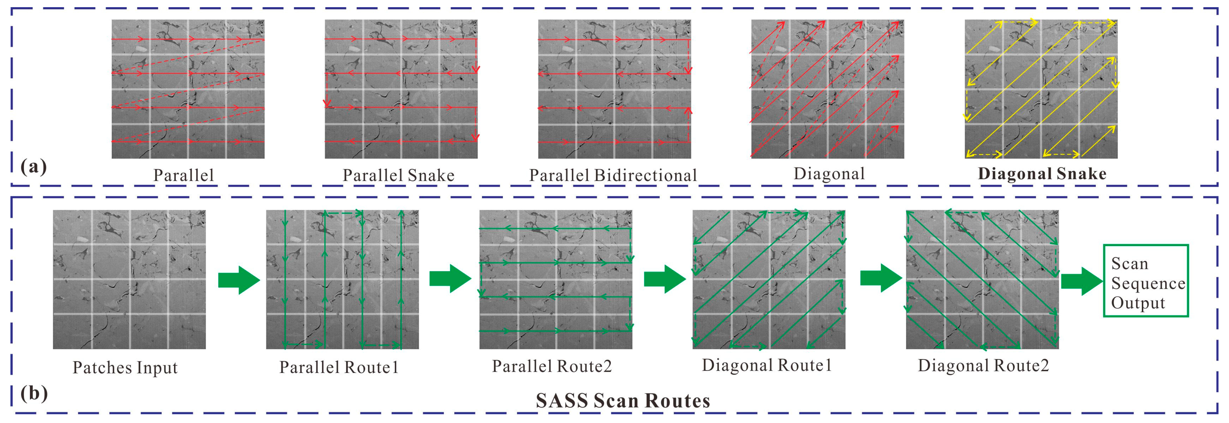
Figure 2. Illustration of SASS and baseline scanning strategies. (a) Four commonly used single-route scan patterns alongside the diagonal snake route of SCSegamba. (b) Execution flow of the SASS scan routes.
Fractalfract 10 00179 g002
Figure 3. Overview of our 2.5D SCSegamba framework. (a) displays the overall network architecture of 2.5D SCSegamba and the workflow for FIB-SEM pore image segmentation. (b) illustrates the structure of our proposed SFIA block.
Fractalfract 10 00179 g003
Figure 4. The workflow of constructing pore surface 3D point cloud from FIB-SEM slices. (e) shows the stacking of raw FIB–SEM images. (f) presents the corresponding binary pore segmentation masks generated by the 2.5D SCSegamba model. In panel (g), the segmented pore pixels are converted into a discrete point set representation for each slice. Finally, (h) illustrates the 3D pore surface point cloud reconstructed via coordinate mapping and neighborhood-based boundary identification algorithm. Panels (ad) provide magnified views of the Regions of Interest (ROI) indicated by the red dashed boxes and arrows in the bottom row.
Fractalfract 10 00179 g004
Figure 5. SEM evidence for pore types and microfractures in Kong 2 shales. (AD) interparticle pores; (E,F) intraparticle dissolution-related pores; (G) intercrystalline pores; (H) OM pores; (I) OM-related shrinkage microfracture along the clay–OM interface. Well and depth information for each panel are provided as follows: (A) (Well G-1, 3148.48 m), (B) (Well G-1, 3078.47 m), (C) (Well G-2, 3891.19 m), (D) (Well G-2, 3857.73 m), (E) (Well G-3, 4123.10 m), (F) (Well G-1, 3187.53 m), (G) (Well G-2, 3857.73 m), (H) (Well G-1, 3187.53 m), (I) (Well G-1, 3078.47 m). Mineral abbreviations: Q, quartz; F, feldspar; D, dolomite; C, calcite; Clay, clay minerals; OM, organic matter.
Fractalfract 10 00179 g005
Figure 6. Low-pressure N2 adsorption characteristics of representative Kong 2 shale samples from three rock types. (AC) N2 adsorption–desorption isotherms (adsorbed volume vs. relative pressure, P/P0). (DF) Incremental pore volume distributions versus pore width. (GI) Differential pore volume distributions (dV/dD) versus pore width. (JL) Cumulative pore volume versus pore width. Panels (A,D,G,J) represent clay-enriched mixed shale; (B,E,H,K) represent siliceous shale; and (C,F,I,L) represent calcareous shale.
Fractalfract 10 00179 g006
Figure 7. FHH fractal plots derived from N2 adsorption isotherms for representative Kong 2 shale samples. Linear regressions used to calculate D1 (low-P/P0 segment) and D2 (high-P/P0 segment) are shown for (a) S-3 (G-1 well, 3303.70 m; clay-enriched mixed shale), (b) S-14 (G-1 well, 2953.28 m; siliceous shale), and (c) S-35 (G-3 well, 4121.30 m; calcareous shale).
Fractalfract 10 00179 g007
Figure 8. Incremental pore-throat size distributions derived from MIP for representative Kong 2 shale samples of three rock types. (a) Clay-enriched mixed shale, (b) siliceous shale, and (c) calcareous shale. Curves show incremental intrusion volume as a function of pore-throat diameter.
Fractalfract 10 00179 g008
Figure 9. Box-counting fractal analysis of 3D pore surface. ε values used for box counting: 2, 3, 5, 7, 10, 15, 23, 34, 51 (generated from a geometric progression with r = 1.5, rounded to integers). (a) Clay-enriched mixed shale (Well G-1, depth 3148.49 m), (b) siliceous shale (Well G-1, depth 2953.28 m), (c) calcareous shale (calcite-dominated; Well G-3, depth 4121.31 m), and (d) calcareous shale (dolomite-dominated; Well G-3, depth 4123.11 m).
Fractalfract 10 00179 g009
Figure 10. Relationships of adsorption-derived fractal dimension (D2) and specific surface area (SSA) with key compositional, geochemical, and petrophysical parameters of the Kong 2 shales. (ai) D2 versus (a) clay minerals; (b) quartz + feldspar; (c) dolomite; (d) calcite; (e) TOC; (f) S1; (g) SSA; (h) pore volume; (i) MIP-estimated permeability. (jo) SSA versus (j) clay minerals; (k) quartz + feldspar; (l) dolomite; (m) calcite; (n) TOC; (o) S1. Symbols are colored by rock type (clay-enriched mixed shale, siliceous shale, and calcareous shale).
Fractalfract 10 00179 g010
Figure 11. Visual comparison of pore segmentation results. (a) Raw FIB-SEM image showing the complexity of pore structures (elongate interparticle pores along mineral grain boundaries, irregular pores at the interface between organic matter and minerals, and small, isolated dissolution pores) and curtaining artifacts. (b) Ground truth annotated by experts. (ce) Segmentation results produced by (c) nnU-Net, (d) SCSegamba, and (e) our proposed 2.5D SCSegamba. The yellow, green, and blue boxes highlight, respectively, missed fine-scale structures and artificial discontinuity of elongate pores, the erroneous identification of organic matter, and missed isolated pores.
Fractalfract 10 00179 g011
Figure 12. Traditional 3D reconstruction and visualization of the lacustrine shales pore system from FIB-SEM slices. (ad) Grayscale 3D FIB–SEM reconstructions with segmented pore space (blue), showing the reconstructed pore system for: (a) clay-enriched mixed shale (Well G-1, depth 3148.49 m, S-7), (b) siliceous shale (Well G-1, depth 2953.28 m, S-14), (c) calcareous shale (calcite-dominated; Well G-3, depth 4121.31 m, S-35), and (d) calcareous shale (dolomite-dominated; Well G-3, depth 4123.11 m, S-36). (a1d1) 3D visualizations of the reconstructed pore system, where individual connected pore clusters (connected components) are distinguished by different colors. (a2d2) Enlarged views of the boxed regions in (a1d1), highlighting local pore system geometry and connectivity.
Fractalfract 10 00179 g012
Figure 13. 3D pore size distribution (equivalent diameter) of different shale lithofacies from FIB–SEM reconstruction. (a) Clay-enriched mixed shale (Well G-1, depth 3148.49 m), (b) siliceous shale (Well G-1, depth 2953.28 m), (c) calcareous shale (calcite-dominated; Well G-3, depth 4121.31 m), and (d) calcareous shale (dolomite-dominated; Well G-3, depth 4123.11 m).
Fractalfract 10 00179 g013
Table 1. Performance evaluation of the proposed method against competitive models on the self-built dataset.
MethodsRecallPrecisionF1mIoU
nnU-net (3D)0.88360.91130.89730.8921
SCSegamba0.90160.88020.88980.8862
2.5D SCSegamba0.93010.93980.93490.9241
Table 2. Sensitivity of 3D pore surface fractal dimension (D) to segmentation perturbations and traditional reconstruction.
Sample IDD (Point Cloud)Erosion (1 Voxel)Dilation
(1 Voxel)
Boundary
Flip 0.5%
D (Traditional)
S-72.61072.5989 (−0.45%)2.6212 (+0.40%)2.6295 (+0.72%)2.1342 (−18.25%)
S-142.46392.4543 (−0.39%)2.4728 (+0.36%)2.4815 (+0.71%)2.0519 (−16.72%)
S-352.33682.3290 (−0.33%)2.3454 (+0.37%)2.3529 (+0.69%)2.0336 (−12.98%)
S-362.52182.5115 (−0.41%)2.5316 (+0.39%)2.5399 (+0.72%)2.0629 (−18.20%)
Disclaimer/Publisher’s Note: The statements, opinions and data contained in all publications are solely those of the individual author(s) and contributor(s) and not of MDPI and/or the editor(s). MDPI and/or the editor(s) disclaim responsibility for any injury to people or property resulting from any ideas, methods, instructions or products referred to in the content.