Added Value for Urban Heat Island Quantification from Machine Learning Downscaling of Air Temperatures

Abstract

The urban heat island effect is well recognized and has been quantified using ground observations within and outside urban areas. Earth Observation has further revealed small-scale local spatial differences, especially in urban surface temperatures, that have been shown to be highly correlated with differences in the urban fabric. However, surface temperatures do not directly translate to human-experienced temperatures, and hence high-resolution air temperature data is of high relevance. However, air temperature is not easily measured from space, and seldom do ground measurements allow for small-scale differences to be quantified to a satisfactory degree. In the present study, we assessed the added value of an air temperature product downscaled using machine learning compared to the high-resolution reanalysis model that formed its foundation. The downscaled product was developed using satellite data, local observations from privately owned weather stations, and high-resolution reanalysis. The comparison focused on Denmark’s four largest urban areas and examined the two data product’s ability to describe the urban heat island effect at the city scale as well as intra-city differences in air temperatures. Both data products show similar urban heat island effects at the city scale, while the downscaled product shows greater intra-city variance in air temperature, with patterns that are somewhat correlated with both urban density and urban green spaces. Generally, the downscaling product offers city planners a better data basis for evaluating where to prioritize contingency and mitigation measures within the urban space.

1. Introduction

The urban heat island (UHI) effect has been recognized for a long time [1,2], with the first reports of a temperature anomaly within a city (London) in 1818 by Luke Howard [3]. Since then, it has been a recurrent topic when discussing human modification of the local climate [4,5], and is adding to the challenge of securing livable local climate conditions in megacities across the globe now and in future climates [6,7,8,9]. Megacities are characterized by very large connected urban agglomerations presenting widespread changes to the surface fabric with marked changes in albedo, heat capacity, permeability, and evaporation potential compared to natural landscapes [10,11]. These changes have been shown to affect local climate conditions [12,13], where elevated temperatures, compared to corresponding rural areas, have the most direct effect on people’s lives and health [14,15], a situation also deemed more critical due to population density in these areas, along with aging population trends.

The UHI effect generally describes the excess heating that cities experience compared to rural areas, whether related to air temperature or surface temperatures [2]. For health effects, the air temperature is most relevant [14], and studies comparing observed in situ data between urban and rural sites show this correlation well [2]. While several metrics exist that try to quantify the spatial extent and severity of UHI effects, they often rely on sparse observations or reanalysis data and can only show UHI effects for typical medium-to-large cities [16]. The alternative is often tailored models developed for forecast purposes, where the lack of local stations makes it hard to quantify the actual precision and where transferability requires understanding of and tailoring to local conditions [17].

More recently, satellite missions have provided a wealth of relevant data regarding surface temperature (e.g., the ESA LST CCI; [18]) that are well measured from satellites through thermal and infrared sensors, and many more recent studies rely on quantifying the UHI effect related to surface temperatures based on satellite products [19,20]. For urban application, the main challenge with satellite data is spatiotemporal resolution: most satellite products do not meet relevant spatiotemporal scales for direct use in urban applications, as they typically either offer high spatial or high temporal resolution, but not both simultaneously [21,22]. Hence, many studies showcase the value of downscaling satellite products to scales relevant in the urban context [23]. Machine Learning (ML) approaches are at the forefront of this development, thanks to their flexibility in terms of scaling factor and limited computational overhead [24,25].

These developments have led to more studies on UHI that utilize either the possibilities of satellite data, high-resolution physically based models, the power of ML, or a combination thereof, and do not restrict themselves to megacities [21,24,26,27,28,29]. These studies show that while the UHI effect might be largest and best described for megacities, it is also relevant for medium-sized cities and thus areas that today cover half of the world’s population today and expected to gain a much larger share in the future [30]. It is also evident that downscaling through ML [27] and using physically based models [28,29] result in quantitative descriptions of the local climate of similar quality, and that the dynamics of air and surface temperature are not necessarily the same [31].

The present study aimed at evaluating a machine learning downscaled product—developed using satellite data, local observations from privately owned weather stations, and a national high-resolution reanalysis [32]—against its driving reanalysis model [33]. The comparison focused on their ability across Denmark’s four largest urban areas.

2. Materials and Methods

2.1. Data

Two different datasets on air temperature 2 m above the surface (t2m) were compared: estimates of Danish weather at 2.5 km resolution based on the DANRA reanalysis system [33], and high-resolution estimates of air temperature based on C4C model outputs [32]. The two datasets are described more in-depth in

Table 1. Description of the datasets compared for UHI quantification.

Name	Spatial Resolution and Coverage	Temporal Coverage	Description	Reference
DANRA	2.5 km on a rotated grid covering a large share of Northern Europe.	Temporal coverage: 1991–2023. Output on hourly time scale. 3-hourly values for the period 2019–2023 are used in this study for full overlap with the C4C dataset.	DANRA, the high-resolution Danish Reanalysis dataset produced by the Danish Meteorological Institute is a dataset specifically made to better represent historical high-resolution weather conditions over Denmark.	[33]
C4C	0.002 × 0.002° (approximately 150 m × 250 m in Denmark) on a regular grid covering the four functional urban areas (FUAs) [34] around the four largest cities in Denmark (Copenhagen, Odense, Aarhus and Aalborg).	Temporal coverage: 2019–2023. Output on 3-hourly resolution.	A Machine Learning based (Random Forest) downscaling product of DANRA developed in the CLIM4cities project. The machine learning-based downscaling was achieved by combining quality-controlled (QC) crowdsourced Netatmo weather observations with satellite observations based geospatial predictors for UHI. The model, the data going into it, and the full validation of it are described thoroughly in Castro et al. [32].	[32]

.

The four Danish functional urban areas (FUAs) examined in this analysis from EUROSTAT [34] cover the four largest urban areas of Denmark: the greater Copenhagen Metropolitan Area and the three cities of Odense, Aarhus, and Aalborg. In regard to size, they differ a lot: the greater Copenhagen Metropolitan Area has around 1.4 million inhabitants in a large connected urban area, whereas Aalborg, the smallest city, has around 120 thousand inhabitants. Aarhus and Odense are in between, but closest to Aalborg in size. In this study, we focused on the urban cores within the FUAs and on the different datasets’ ability to perform exactly there, compared to the analyses in Castro et al. [32], which evaluated performance across the full FUAs.

For validation, the Netatmo dataset used for validating C4C in Castro et al. [32] is utilized here for the same purpose. Approximately 5000 stations are available across the four FUAs, and data for 2023 have been reserved for validation of C4C in Castro et al. [32], and is again utilized for validation here.

To further explore the intra-city differences observed, further static satellite-based datasets are used. Specifically, impermeability density and treetop cover-density data were retrieved from the Copernicus Land Monitoring Service and European Environment Agency [35,36].

2.2. Methods

In order to evaluate the performance of the two models in urban centers, comparison against a Netatmo validation dataset not previously seen by the models for 2023 was used to calculate the absolute deviation between models and observations. For each Netatmo station, a simple deviation was calculated against the closest model grid value for each timestep (t):

$$Deviation=T_t^{model}-T_t^{Netatmo}$$

(1)

The deviations were then split in seasons and cities in order to distinguish when and where which models performed better.

To quantify the UHI effects of each FUA at the city scale, urban center fields (UF) and corresponding rural reference fields (RF) were defined. The fields are a means of defining equal-size urban and rural areas for comparison irrespective of the resolution of the underlying datasets and irrespective of the actual urban form. A field size of 0.1 × 0.1° was chosen to capture the city centers without too much interference from surrounding sub-urban and rural areas. The dataset on impermeability density was used to center the urban fields in the areas with highest density, and the rural fields in areas with low density.

The UHI effect (UHIe) was quantified for each timestep (t) for each city (c) as the mean difference between the urban field and the rural field:

$$UHI{e}_t^c=mean\left(U{F}_t^c\right)-mean\left(R{F}_t^c\right)$$

(2)

where the mean was taken over each field to ensure a fair comparison between the DANRA and C4C datasets, which have a significantly different spatial resolution, see Section 2.1.

As the UHIe time series for each city is in high temporal resolution, the index was calculated for a number of representative subsamples of the data:

• Extended summer season (May–September): UHIe(Summer).
• Extended winter season (November–March): UHIe(Winter).
• The 3% warmest days based on the average daily temperature across Denmark in the DANRA dataset: UHIe(Top 3%).
• The 3% coldest days based on the average daily temperature across Denmark in the DANRA dataset: UHIe(Bottom 3%).

The choice of using extended summer and winter seasons was based on the limited temporal coverage of the C4C dataset (5 years) in order to make the best possible use of the available data. The “3% warmest days” subsample corresponds roughly to the national average estimate of number of warm-wave days (defined as three consecutive days with maximum temperature exceeding 25 °C) in the current climate, as reported in the Danish Climate Atlas (Klimaatlas.dk, accessed on 15 February 2026). As such, this includes all days where health effects of heat exposure are expected to start appearing. In line with the WMO [37], we did not apply the warm-wave days threshold directly, but opted for a simpler percentile approach as Denmark has no official definition of cold-wave days, and the same number of days as for warm-wave days were chosen for consistency (55 days in total for each selection).

In order to characterize the internal field variation for UFs and RFs, the difference between the 95th percentile (q95) and the 5th percentile (q05) values in any grid point within the fields was calculated for each timestep (t):

$$\Delta T_t^c=q\mathsf{95}\left(fiel{d}_t^c\right)-q\mathsf{05}\left(fiel{d}_t^c\right)$$

(3)

Given the spatial resolution difference between DANRA and C4C, the data basis for calculating this index varied significantly, with approximately 15 and 2500 grid points within a 0.1 × 0.1° field for DANRA and C4C, respectively.

3. Results and Discussion

3.1. Urban Centers and Reference Rural Areas

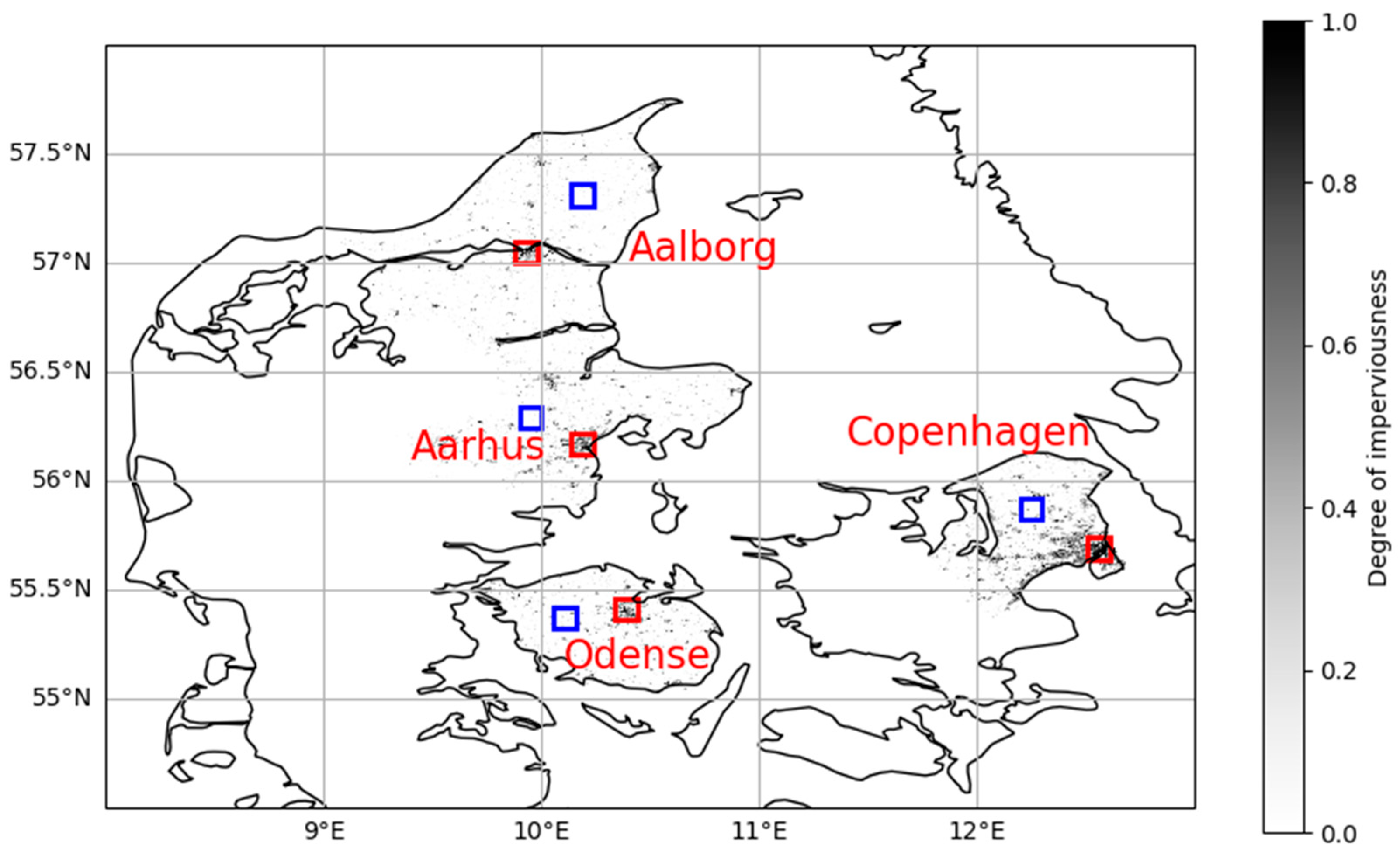
Based on the dataset on imperviousness, city centers and reference rural fields are defined for each investigated FUA as 0.1 × 0.1° cells (

Table 2. Coordinates of urban and rural reference fields. Each set of coordinates mark the center of a 0.1 × 0.1° cell.

	Urban Reference Field Center (lon; lat)	Rural Reference Field Center (lon; lat)
Copenhagen	12.56; 55.69	12.25; 55.87
Odense	10.39; 55.41	10.11; 55.37
Aarhus	10.19; 56.17	9.95; 56.29
Aalborg	9.93; 57.05	10.19; 57.31

). The resulting areas can be seen in Figure 1, where red squares mark the urban areas and blue squares mark the rural areas. For Copenhagen, finding a rural area of the required size completely free of small towns, lakes, or forests proved to be difficult. Ultimately, an area dominated by farmland was selected. For the other three FUAs, the city centers are surrounded by significantly more farmland, making it much easier to find suitable reference rural areas. For that reason, other alternatives could have been chosen with little influence on the results.

3.2. Validation of Datasets Against Independent Observations

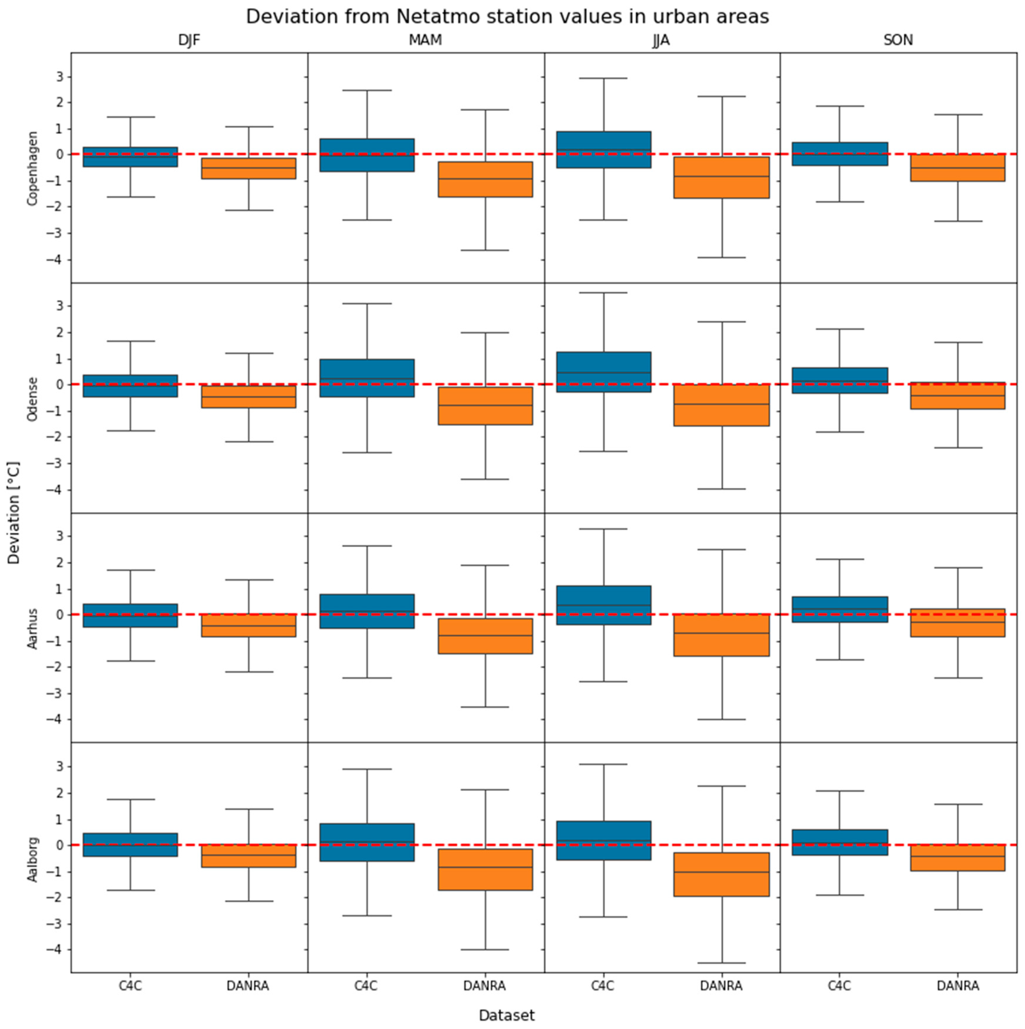
The superior performance of C4C against DANRA across the full FUAs is demonstrated in Castro et al. [32]. Here, we focus on evaluating the performance within the urban reference fields described in Table 2. For that purpose, between 70 and 110 Netatmo stations are available within each field, and data from 2023 not previously seen by the model are used for validation. Figure 2 displays the deviations between DANRA and C4C against Netatmo (Equation (1)). DANRA consistently has a cold bias in the city centers compared to the Netatmo stations, and C4C seems to correct that with a mean bias close to 0 °C for all seasons and cities. For spring and summer, this correction is quite large, as more than 75% of the DANRA values have a negative bias. Other than that, both datasets have similar spreads within each season–city combination, but C4C never shows a larger spread in absolute values compared to DANRA.

3.3. Diurnal Urban Heat Island Effect at City Scale

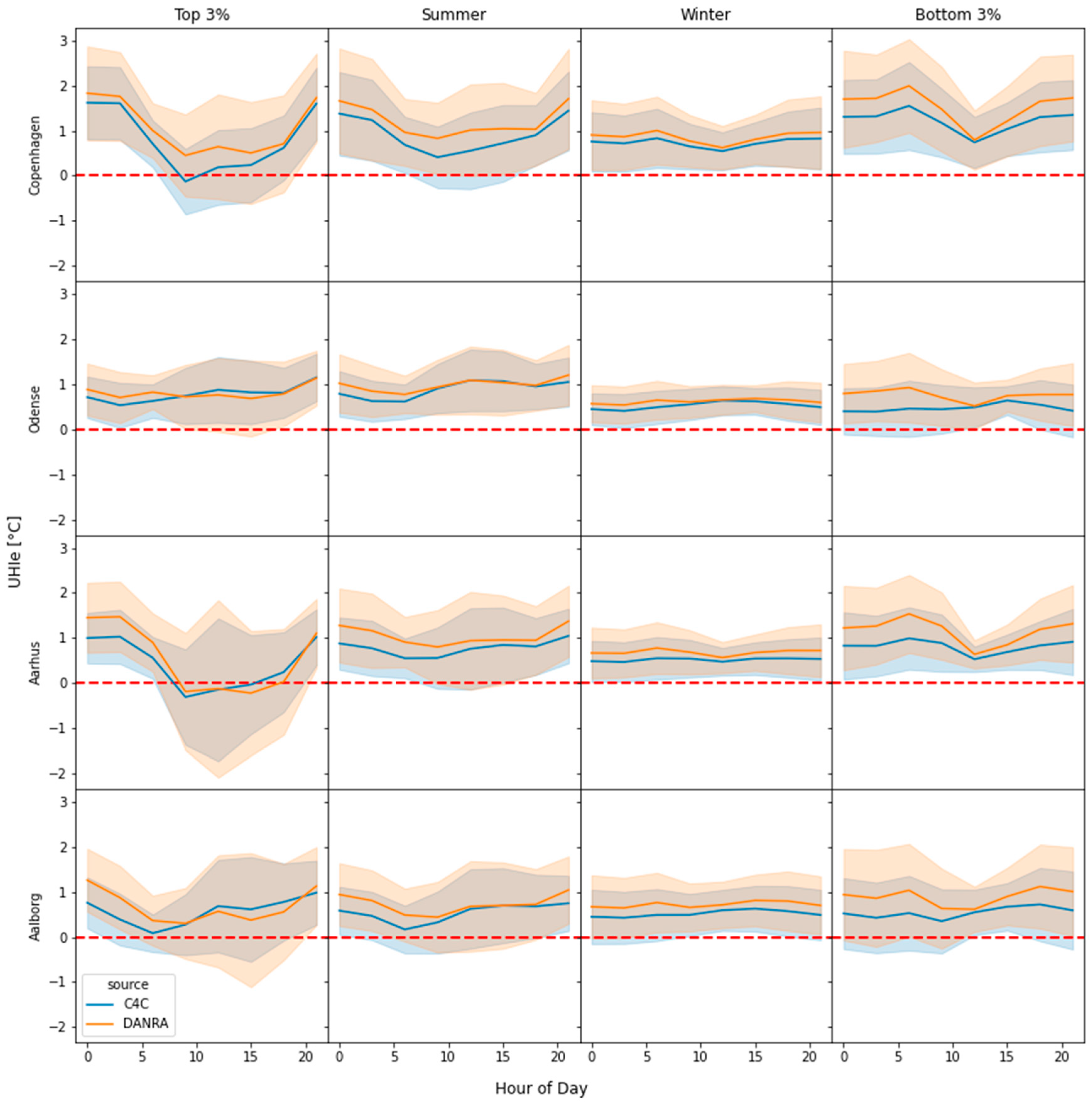
No clear differences are detectable between DANRA and C4C with regard to the citywide UHI effect (Figure 3, Equation (2)). This is actually a bit surprising, given the cold bias shown in Figure 2. A diurnal cycle appears to be present in Copenhagen during the summer season, but this is more or less absent for the three other cities. For the winter season, there does not seem to be any diurnal cycle for any of the cities. For the 3% hottest days, the UHI effect peaks during nighttime in most cities. For the 3% coldest days, similarities between the patterns of DANRA and C4C are also seen, but DANRA seems to consistently result in higher UHIe values for all cities. In general, the calculated UHI effects are more stable over the day in winter, and the spread seems to be largest for the extreme cases (both hot and cold). In all, both datasets show clear positive UHIe signals across all evaluated scenarios, the effect being most pronounced during hot extremes, and DANRA having a slightly stronger UHIe signal at citywide scale than what is observed for C4C.

3.4. Intra-Field Differences in Temperature

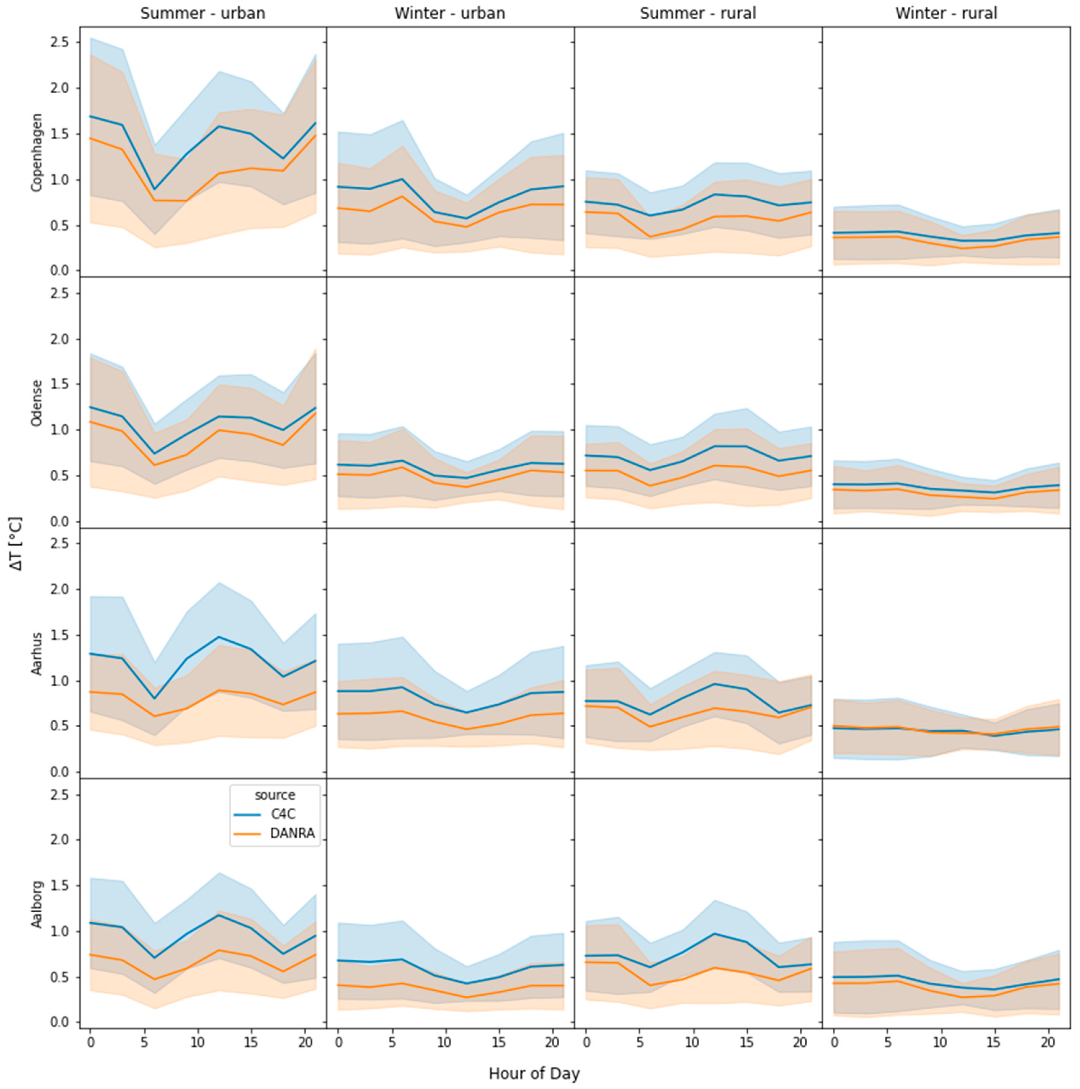
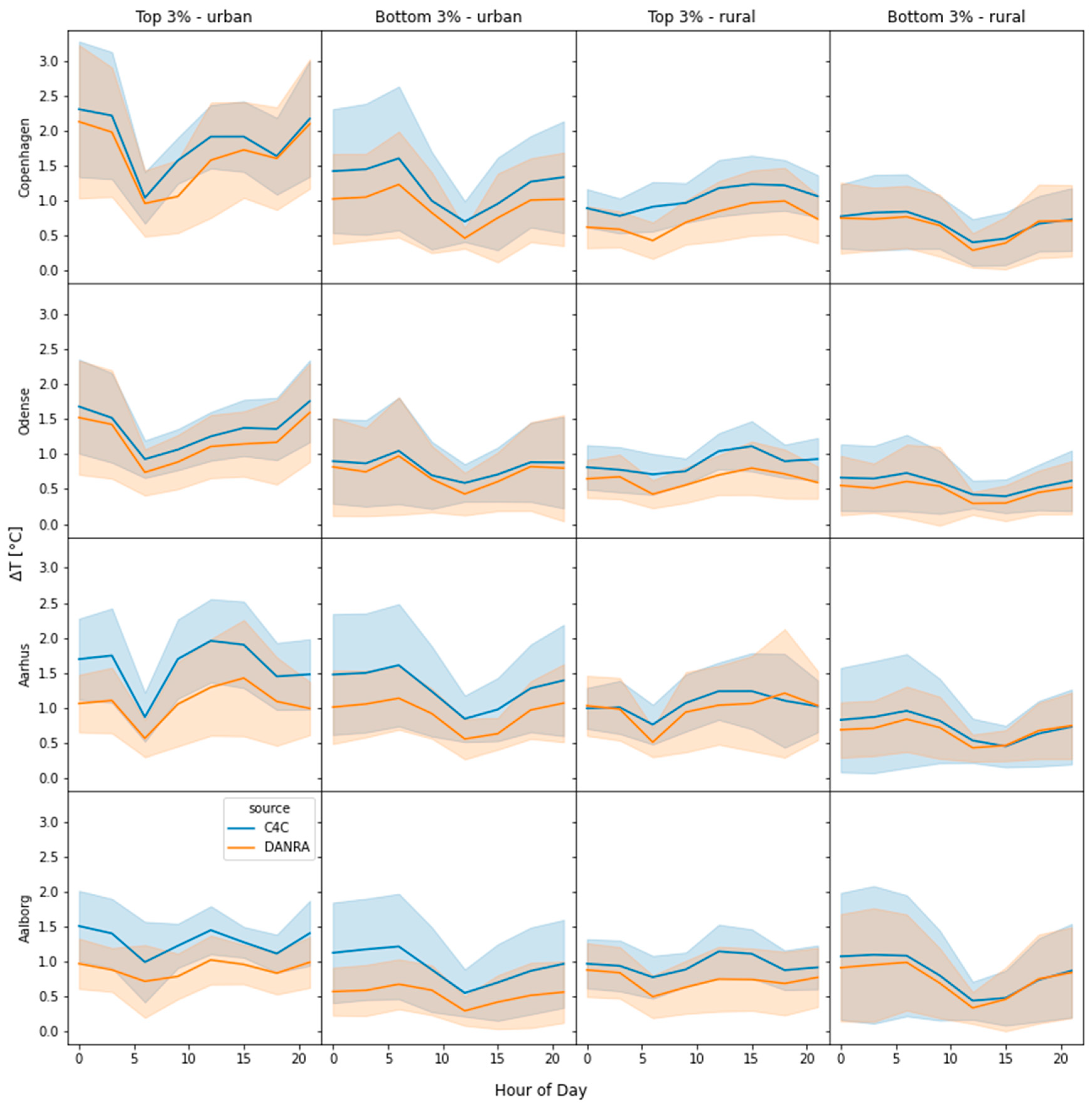
Looking at the intra-field difference expressed through the ΔT values in Figure 4 (Equation (3)), it seems that C4C has larger variations within the 0.1 × 0.1-degree fields than DANRA, especially concerning the urban summer values. In contrast, the rural winter values are almost identical between the two datasets, showing that the more uniform expectations for these fields are probably a correct assumption. This is not surprising, given the resolution difference between the two data products, but it is striking how consistently the effect is seen to materialize between winter and summer and between rural and urban contexts. It is also noteworthy how pronounced the effect is during urban summer. This agrees with the known influence of larger day-night variations in explaining the thermal signature of the urban fabric. This demonstrates that C4C resolves local temperature-influencing features to a much larger extent than DANRA, despite the city-average UHIe being lower than that seen in DANRA (Figure 3). Also, knowing that the average bias is smaller for C4C compared to DANRA as reported in Figure 2, despite the larger spread of values, confirms this as a more realistic behavior than the one observed for DANRA. Figure 5 reports the same results for the top and bottom 3% scenarios. Here, the most obvious result is that the largest differences are seen for the urban fields of the coastal cities of Aarhus and Aalborg, where the C4C dataset shows much larger variation than DANRA. Besides this, C4C seems to produce slightly higher intra-field differences than DANRA, and the effect is most pronounced for the urban fields and for the extremes, although the warm extremes for the rural reference fields for Copenhagen and Odense also seem to have significantly more intra-field variability in C4C compared to DANRA.

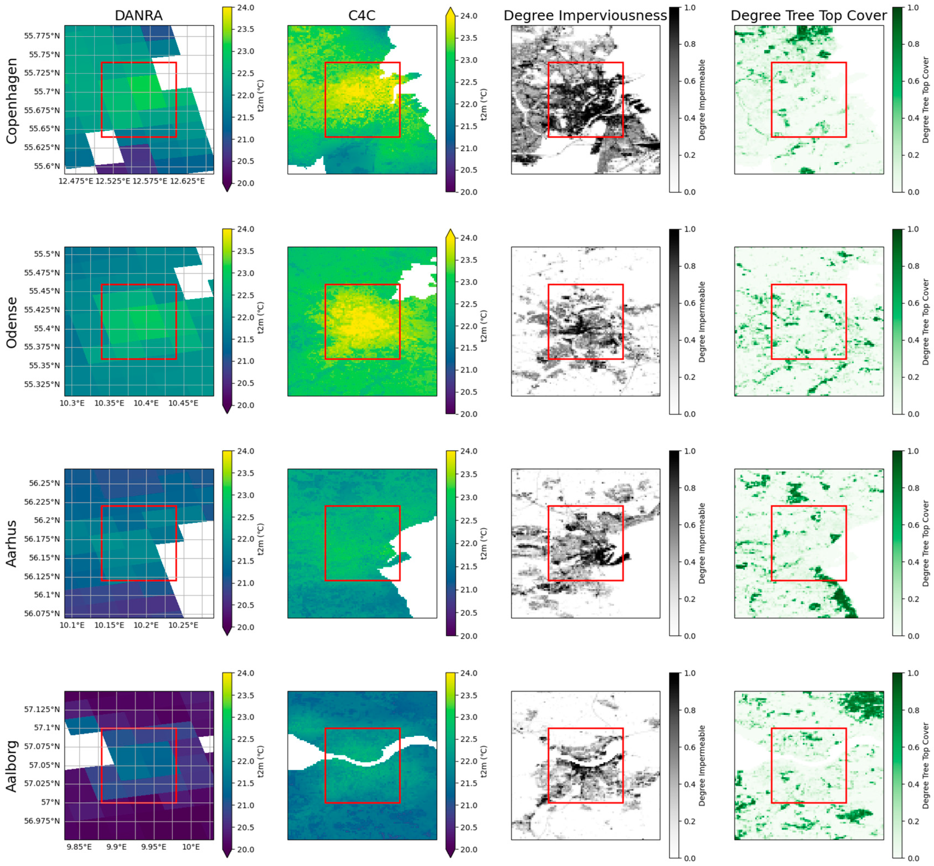
3.5. Understanding the Intra-Field Differences in Temperature

Figure 6 shows the average temperature of the 3% hottest days for the four city fields along with maps of imperviousness densities and treetop densities. For Copenhagen, DANRA captures much of the urban form, as the dense urban area is large enough to be represented somewhat adequately at the kilometer-scale resolution of the model. The large forest north of the city near the coast is also seen in DANRA, but other green features do not seem to have enough volume to have an influence. C4C resolves these better, and especially west and northwest of the city field, where a more accurate representation of the anticipated impacts of greening on the temperature can be seen. Odense highlights the same conclusions as for Copenhagen: C4C neatly shows the cooling effects that the green river belts, going into the city from west and south towards the sea, have on the local temperature. For a city of this size, DANRA seems to be at a relatively low resolution, failing to capture any local features. DANRA is limited to representing that the city center suffers from a UHI effect, which steadily decreases as one moves away from the city center. Aarhus and Aalborg appear to exhibit somewhat similar effects: urban centers of this size and close to water are not convincingly captured by DANRA. Furthermore, C4C seems to better capture the expected cooling effects of green areas than the warming effects of the city. This suggests that these less dense small-extent city centers at the waterfront do not produce as strong a UHI signal as the even smaller town of Odense, which in turn is less influenced by water. For all cities, the C4C dataset does capture local features expected to impact the local temperature, and thereby resolves features that are relevant from a mitigation planning perspective (e.g., how large a green area must be to produce a measurable effect), as well as for a contingency perspective (where the cool places are to send people to). This demonstrates the value of downscaling the already very well-performing DANRA model to sub-kilometer scale.

The urban and rural fields (UFs and RFs) capture well most of the three smaller cities (Odense, Aalborg, and Odense), but only the core city center of Copenhagen (see Figure 6). As such, one could argue that a common field size is not ideal between the investigated FUAs, and different-sized fields would likely influence the results; however, given the difficulty in finding a suitable rural field near Copenhagen, a larger field is probably not feasible. In the end, the field size chosen is the best possible compromise between ensuring a sufficiently large area to average over while excluding smaller towns.

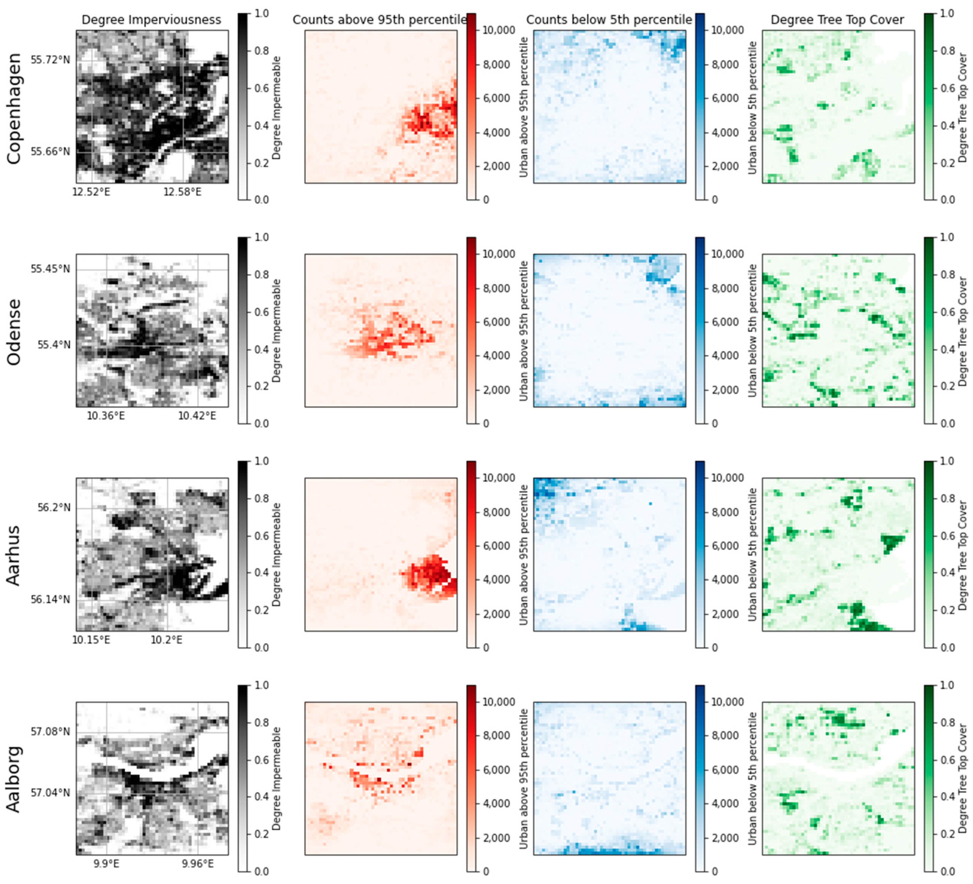
In Figure 7, we count the number of times the temperature in each grid cell is above the 95th percentile measures in a given timestep (below the 5th percentile), corresponding to the percentiles used for calculating ΔT. The warm extremes are compared to the degree of imperviousness and the cold extremes to the degree of treetop cover. For Copenhagen, there is a strong coincidence between grid points that are very often hotter and some of the densest areas of the city: there are, however, other equally dense areas of the city that do not show up in this comparison, so clearly other variables play a role as well. For the coldest areas, the coincidence is strong with the large green area just south of the city center, but smaller green areas closer to the dense city do not seem to cool to a degree that is captured here. For Odense, the correlation is much less clear. The hottest grid cells are within the city core, but not necessarily the densest parts of the city. Likewise, the coolest grid cells are not heavily correlated with the green parts of the city, but rather seem to be furthest away from the hot inner city. As such, Odense seems to show a textbook example of UHI shape, with a somewhat circular hot area in the center and a cooling gradient as one moves away. For Aarhus, the hottest grid cells are concentrated in the dense inner city at the harbor front, an area very poorly captured by DANRA as it is not recognized as a land cell here. The coldest grid cells correlate well with the largest green areas in and around the city, as well as the rural area in the northwest corner of the area. Finally, Aalborg has very few explainable patterns compared to the other cities. The hottest cells are in the city center and along the old industrial harbor front, but are much less connected than what is observed in the other cities. The coolest grid cells are spread all over the city and show very little correlation with the green areas.

Comparing the results to the most recent available land surface temperature heat maps reported by Alexander [26], some clear differences are observed. Overall, for all four cities, their maps show much closer correlations with city density and green spaces than our results. For Copenhagen, the hottest areas are clearly different in the two analyses. While we observe air temperatures to be hottest north of the city center, she observes land surface temperatures to be highest south of the city center, close to the large green area. This clearly highlights that the two are not mutually interchangeable and that the large green area has a clear cooling effect on the nearby dense urban area when it comes to air temperature. For Odense, the results are on one hand the most similar of the four cities, but on the other hand small-scale differences between dense city and urban nature are expressed to a very detailed degree in the land surface temperature maps, but not picked up in the air temperature data. As such, the correlation with city density and green spaces is very pronounced in [26] and not a very good descriptor for the air temperature dataset, even though the overall form of the heat maps has many similarities. For Aarhus and Aalborg, the results between [26] and our results are quite different. Aalborg in general has much more variation in land surface temperature compared to air temperature, and thus also more pattern-correlated with the city density and urban greenspace. The signal in air temperature observed in Figure 5 with the hottest areas along the harbor front is also seen in the land surface temperature map, but other areas of the city are as hot as well, making the pattern very different. For Aarhus, the city center is not particularly hot in [26], and the pattern is neither as strongly correlated with urban density as for the other cities. The strongest agreement between the two datasets is related to the cooling effects of the larger green areas, which is pronounced in both datasets. It should be noted that the temporal scope of the two datasets does not overlap and the spatial resolution is different. A direct quantitative comparison is therefore not performed, as the conclusions drawn from such a comparison would be very hard to justify.

Comparing the results to a study by Wang et al. [28], the observed UHI effects are comparable to what they modeled at 300 m and 3 km scales for similarly sized high-latitude Swedish cities. They did not see large differences between the kilometer-scale and the even finer scale either, although the finer scale showed clear improvement in spatially resolving local urban features, as well as representing observed differences during individual events. For Copenhagen, comparison to the UrbClim results reported by Lauwaet et al. [38] show that the citywide UHI effect they report is generally lower than what is observed in our study. This is the case even though their approach should include a large proportion of the inter-city variability on top of the mean effect, as they rely on the 90th percentile. This clearly highlights the added value from having a machine learning-downscaled dataset informed by local weather observations, and suggests that the C4C dataset is an excellent data basis for city planners to use when evaluating where to prioritize contingency and mitigation measures within the urban space.

4. Conclusions

This study evaluated the added value of a high-resolution ML-based downscaling method (C4C) relative to regional reanalysis, DANRA, for quantifying and characterizing the UHI effect in the four largest cities of Denmark. The results demonstrate that although both datasets indicate the presence of a UHI effect signal across different spatial domains, C4C gives a more nuanced spatial representation of air temperature variability.

For all four cities, the UHI effect was strongest during the 3% warmest days, particularly at nighttime, similar to the results shown for comparable Swedish conditions by Wang et al. [28]. Both DANRA and C4C captured the expected diurnal cycle in Copenhagen and Aarhus, but C4C displayed less pronounced citywide UHI intensity compared to DANRA. This likely reflects C4C’s ability to resolve local cooling influences such as vegetation and water bodies, which are smoothed out at coarser resolution. Furthermore, the use of quality-controlled (QC) crowdsourced weather observations from the cities allowed for the inner-city temperature amplification on the hottest days to be explicitly used for the ML downscaling. This in turn made the C4C model able to capture the large inter-city variability actually observed and not represented well in DANRA. As such, the most notable distinction between the two datasets emerged from the intra-field temperature differences, where C4C consistently revealed greater spatial variability at small scales not represented well by DANRA. This effect was negligible for winter rural fields, but otherwise robust across seasons, times of day, and land cover types. The spatial variability may again be attributed to the use of high-density crowdsourced observations combined with geospatial indicators for the ML downscaling. This approach effectively captures how urban land use, and thus near-surface temperature, can change significantly over short distances.

In conclusion, while both products offer valuable insights for general UHI assessment, the C4C dataset provides added value in identifying intra-urban variability and capturing local features relevant for urban planning, contingency, and heat mitigation.

References

1. Bornstein, R.D. Observations of the Urban Heat Island Effect in New York City. J. Appl. Meteorol. 1968, 7, 575–582. [Google Scholar] [CrossRef]
2. Oke, T.R. The urban energy balance. Prog. Phys. Geogr. Earth Environ. 1988, 12, 471–508. [Google Scholar] [CrossRef]
3. Howard, L. The Climate of London. IAUC Edition. 2007. Available online: https://urban-climate.org/wp-content/uploads/2023/03/LukeHoward_Climate-of-London-V1.pdf (accessed on 14 February 2026).
4. Lowry, W.P. Empirical estimation of urban effects on climate: A problem analysis. J. Appl. Meteorol. Climatol. 1977, 16, 129–135. [Google Scholar] [CrossRef]
5. Oke, T.R. The energetic basis of the urban heat island. Q. J. R. Meteorol. Soc. 1982, 108, 1–24. [Google Scholar] [CrossRef]
6. Bohnenstengel, S.I.; Evans, S.; Clark, P.A.; Belcher, S.E. Simulations of the London urban heat island. Q. J. R. Meteorol. Soc. 2011, 137, 1625–1640. [Google Scholar] [CrossRef]
7. Lemonsu, A.; Viguié, V.; Daniel, M.; Masson, V. Vulnerability to heat waves: Impact of urban expansion scenarios on urban heat island and heat stress in Paris (France). Urban Clim. 2015, 14, 586–605. [Google Scholar] [CrossRef]
8. Raj, S.; Yerim, L.; Yun, G.Y.; Santamouris, M. Contrasting urban heat disparities across income levels in Seoul and London. Sustain. Cities Soc. 2025, 121, 106215. [Google Scholar] [CrossRef]
9. Shaker, R.R.; Altman, Y.; Deng, C.; Vaz, E.; Forsythe, K.W. Investigating urban heat island through spatial analysis of New York City streetscapes. J. Clean. Prod. 2019, 233, 972–992. [Google Scholar] [CrossRef]
10. Taubenböck, H.; Esch, T.; Felbier, A.; Wiesner, M.; Roth, A.; Dech, S. Monitoring urbanization in mega cities from space. Remote Sens. Environ. 2011, 117, 162–176. [Google Scholar] [CrossRef]
11. Yue, W.; Liu, X.; Zhou, Y.; Liu, Y. Impacts of urban configuration on urban heat island: An empirical study in China mega-cities. Sci. Total Environ. 2019, 671, 1036–1046. [Google Scholar] [CrossRef]
12. Mills, G.; Cleugh, H.; Emmanuel, R.; Endlicher, W.; Erell, E.; McGranahan, G.; Ng, E.; Nickson, A.; Rosenthal, J.; Steemer, K. Climate Information for Improved Planning and Management of Mega Cities (Needs Perspective). Procedia Environ. Sci. 2010, 1, 228–246. [Google Scholar] [CrossRef]
13. Souma, K.; Sunada, K.; Suetsugi, T.; Tanaka, K. Use of ensemble simulations to evaluate the urban effect on a localized heavy rainfall event in Tokyo, Japan. J. Hydro-Environ. Res. 2013, 7, 228–235. [Google Scholar] [CrossRef]
14. Ge, Q.; Xu, X.; Liu, X. Heat Health Risks. In Atlas of Environmental Risks Facing China Under Climate Change; Springer: Singapore, 2017; pp. 51–108. [Google Scholar] [CrossRef]
15. Loughnan, M.; Nicholls, N.; Tapper, N.J. Mapping Heat Health Risks in Urban Areas. Int. J. Popul. Res. 2012, 2012, 518687. [Google Scholar] [CrossRef]
16. Schwingshackl, C.; Daloz, A.S.; Iles, C.; Aunan, K.; Sillmann, J. High-resolution projections of ambient heat for major European cities using different heat metrics. Nat. Hazards Earth Syst. Sci. 2024, 24, 331–354. [Google Scholar] [CrossRef]
17. Giannaros, T.M.; Melas, D.; Daglis, I.A.; Keramitsoglou, I. Development of an operational modeling system for urban heat islands: An application to Athens, Greece. Nat. Hazards Earth Syst. Sci. 2014, 14, 347–358. [Google Scholar] [CrossRef]
18. Ghent, D.; Veal, K.; Perry, M. ESA Land Surface Temperature Climate Change Initiative (LST_cci): Monthly Multisensor Infra-Red (IR) Low Earth Orbit (LEO) land surface temperature (LST) time series level 3 supercollated (L3S) global product (1995–2020), version 2.00. NERC EDS Cent. Environ. Data Anal. 2022. [Google Scholar] [CrossRef]
19. Bechtel, B.; Demuzere, M.; Mills, G.; Zhan, W.; Sismanidis, P.; Small, C.; Voogt, J. SUHI analysis using Local Climate Zones—A comparison of 50 cities. Urban Clim. 2019, 28, 100451. [Google Scholar] [CrossRef]
20. Wicki, A.; Parlow, E.; Feigenwinter, C. Evaluation and Modeling of Urban Heat Island Intensity in Basel, Switzerland. Climate 2018, 6, 55. [Google Scholar] [CrossRef]
21. Guha, S.; Govil, H.; Mukherjee, S. Impact of seasonality and land use changes on urban heat island using earth-observing satellites. In Earth Observation in Urban Monitoring; Elsevier: Amsterdam, The Netherlands, 2024; pp. 133–153. [Google Scholar] [CrossRef]
22. Singh, S.; Mall, R.K.; Chaturvedi, A.; Singh, N.; Srivastava, P.K. Advances in remote sensing in measuring urban heat island effect and its management. In Earth Observation in Urban Monitoring; Elsevier: Amsterdam, The Netherlands, 2024; pp. 113–132. [Google Scholar] [CrossRef]
23. Chauhan, A.; Wasim Md Mohanty, S.; Pandey, P.C.; Pandey, M.; Maurya, N.K.; Rankavat, S.; Dubey, S.B. Earth observation applications for urban mapping and monitoring: Research prospects, opportunities and challenges. In Earth Observation in Urban Monitoring; Elsevier: Amsterdam, The Netherlands, 2024; pp. 197–229. [Google Scholar] [CrossRef]
24. Kumar, D.; Bassill, N.P. Artificial intelligence for sustainable urban climate studies. In Earth Observation in Urban Monitoring; Elsevier: Amsterdam, The Netherlands, 2024; pp. 291–307. [Google Scholar] [CrossRef]
25. Perikamana, K.K.; Balakrishnan, K.; Tripathy, P. Deep learning approach for monitoring urban land cover changes. In Earth Observation in Urban Monitoring; Elsevier: Amsterdam, The Netherlands, 2024; pp. 171–196. [Google Scholar] [CrossRef]
26. Alexander, C. Influence of the proportion, height and proximity of vegetation and buildings on urban land surface temperature. Int. J. Appl. Earth Obs. Geoinf. 2021, 95, 102265. [Google Scholar] [CrossRef]
27. Oliveira, A.; Lopes, A.; Niza, S.; Soares, A. An urban energy balance-guided machine learning approach for synthetic nocturnal surface Urban Heat Island prediction: A heatwave event in Naples. Sci. Total Environ. 2022, 805, 150130. [Google Scholar] [CrossRef]
28. Wang, F.; Aldama-Campino, A.; Belušić, D.; Amorin, J.H.; Ribeiro, I.; Wiréhn, L.; Segersson, D.; Döscher, R.; Navarra, C.; Neset, T.-S.; et al. Interactions of urban heat islands and heat waves in Swedish cities under present and future climates. Urban Clim. 2025, 59, 102286. [Google Scholar] [CrossRef]
29. Wang, F.; Belušić, D.; Amorin, J.H.; Ribeiro, I. Assessing the impacts of physiography refinement on Stockholm summer urban temperature simulated with an offline land surface model. Urban Clim. 2023, 49, 101531. [Google Scholar] [CrossRef]
30. World Bank. TOPIC—Urban, Resilience and Land. 2025. Available online: https://data360.worldbank.org/en/infrastructure/urban-resilience-and-land (accessed on 7 July 2025).
31. Naserika, M.; Nazarian, N.; Hart, M.A.; Sismanisdis, P.; Kittner, J.; Bechtel, B. Multi-city analysis of satellite surface temperature compared to crowdsourced air temperature. Environ. Res. Lett. 2024, 19, 124063. [Google Scholar] [CrossRef]
32. Castro, M.; Paixão, J.; Girão, I.; Marques, B.; Zeitzen, R.M.K.; Cunha, R.; Thejll, P.; Sørup, H.J.D.; Paletta, Q.; Oliveira, A. Urban Thermal Signal Downscaling: Implementing the Machine Learning Approach in Danish Functional Urban Areas. Prepr. SSRN 2026, 6172920. [Google Scholar] [CrossRef]
33. Yang, X.; Peralta, C.; Amstrup, B.; Hintz, K.S.; Thorsen, S.B.; Denby, L.; Christiansen, S.K.; Schulz, H.; Pelt, S.; Schreiner, M. DANRA: The Kilometer-Scale Danish Regional Atmospheric Reanalysis. arXiv 2025, arXiv:2510.04681. [Google Scholar] [CrossRef]
34. Eurostat. Methodological Manual on Territorial Typologies—Statistics Explained; Eurostat: Luxembourg, 2018. [Google Scholar] [CrossRef]
35. EEA. Imperviousness Density 2018 (Raster 10 m), Europe, 3-Yearly, Aug. 2020; EAA: Copenhagen, Denmark, 2020. [Google Scholar] [CrossRef]
36. EEA. Tree Cover Density 2018—Present (Raster 100m), Europe, Yearly, Nov. 2024; EAA: Copenhagen, Denmark, 2024. [Google Scholar] [CrossRef]
37. WMO. Guidelines on the Definition and Characterization of Extreme Weather and Climate Events; WMO-No. 1310; WMO: Geneva, Switzerland, 2023; Available online: https://library.wmo.int/viewer/58396 (accessed on 1 February 2026).
38. Lauwaet, D.; Berckmans, J.; Hooyberghs, H.; Wouters, H.; Driesen, G.; Lefebre, F.; De Ridder, K. High Resolution Modelling of the Urban Heat Island of 100 European Cities. Urban Clim. 2024, 54, 101850. [Google Scholar] [CrossRef]
Figure 1. The four investigated functional units. Urban reference fields marked in red, Rural reference fields marked in blue (Table 2).
Urbansci 10 00171 g001
Figure 2. Deviations of DANRA and C4C against Netatmo for each season and urban reference field.
Urbansci 10 00171 g002
Figure 3. UHIe calculated for all four cities for all scenarios (the top 3% warmest days, extended summer season (MJJAS), extended winter season (NDJFM), and the bottom 3% coldest days) for both datasets (C4C and DANRA). For both datasets, the mean ± one standard deviation is reported.
Urbansci 10 00171 g003
Figure 4. ΔT calculated for all four cities for summer and winter scenarios for both urban and rural fields and both datasets (C4C and DANRA). For both datasets, the mean ± one standard deviation is reported.
Urbansci 10 00171 g004
Figure 5. ΔT calculated for all four cities for top and bottom 3% scenarios for both urban and rural fields and both datasets (C4C and DANRA). For both datasets, the mean ± one standard deviation is reported.
Urbansci 10 00171 g005
Figure 6. Comparison of the average temperature signal for the 3% hottest days for DANRA and C4C compared to maps of the imperviousness degree and treetop-cover degree for all four cities.
Urbansci 10 00171 g006
Figure 7. Comparison of the degree of imperviousness, counts of times a grid cell is above the 95th (below the 5th) percentile with respect to the intra-field temperature difference within a timestep, and the degree of treetop cover for the four city centers.
Urbansci 10 00171 g007