Cyclist Safety in Complex Urban Environments: Infrastructure, Traffic Interactions, and Spatial Anomalies in Rome, Italy

Abstract

Improving cyclist safety conditions in the urban context is a key strategy to promote sustainable transport modes and reduce noise and environmental pollution. Recent plans have also addressed this point. In September 2020, the UN General Assembly declared the Decade of Action for Road Safety 2021–2030, aiming to reduce the number of road deaths by at least half. To achieve this task and highlight the risk factor, after collecting and pre-processing cyclist crash data in the city of Rome between 2013 and 2020, Random Forest and Ordered Logistic Regression models are proposed. The crash dataset is also enriched with vehicular speed and flows, and geographical information. A DBSCAN Clustering Analysis is also proposed to identify anomalous areas in the city. The findings show that the presence of cycle paths, the presence of anthropic activities, such as shops, schools, and universities, play a risk mitigation role. Conversely, vehicular speed and heavy vehicles emerge as the main detected risk factors. Finally, spatial analysis indicates that commercial activities reduce cycle path safety due to complex interactions with other road users. Furthermore, historic areas present unique risks driven by pedestrian flows and poor road surfaces, despite low vehicular traffic.

1. Introduction

In 2004, the World Health Organization (WHO) launched the World Report on Road Traffic Injury Prevention, stressing, for the first time, the unsustainable and unsafe structure of the road traffic system [1]. This preliminary joint action laid the foundations, several years later, in 2009, of the Decade of Action for Road Safety 2011–2020, as a result of the first Global Ministerial Conference on Road Safety, held in the Russian Federation [2]. Two years later, in 2011, the plan was launched to reverse the unacceptable increase in road deaths [3].

A decade later, in September 2020, the UN General Assembly declared the introduction of a new set of objectives contained in the Decade of Action for Road Safety 2021–2030 [4], with a more precise scope than the previous version. The main aim was to reduce road fatalities by at least 50% through the promotion of sustainable urban mobility, in line with the Stockholm Declaration [5]. At a smaller scale, but with higher expectations, the European Commission proposed a new and ambitious strategy called the EU Road Safety Policy Framework 2021–2030 [6], which aims to reduce to zero the number of road fatalities by 2050.

Despite these efforts made by national and international Governments and Institutions, Road Traffic Injuries are still a critical global health issue. The most exposed to this critical burden are children and young people aged 5–29 years, with 1.19 million deaths worldwide in 2021. Cyclists account for 6% of these fatal crashes, roughly one per 100,000 population [7].

Following this direction, this work aims to understand which factors affect the safety of vulnerable road users (in this case, cyclists) to support the development of safe and sustainable cities. While the current literature review on this topic already highlights the role of road infrastructure, urban environment characteristics, and road users’ characteristics, some research gaps remain. Few studies combine in a coherent framework contextual factors related to the urban environment and road traffic characteristics, which is critical for quantifying cyclist crash severity (degree of harm) and the main contributing factors. In addition to that, the crash dataset is characterized by strong heterogeneity and class imbalance (that means more non-fatal than fatal crashes). While some models are ad hoc, designed to handle heterogeneity (e.g., Partial Proportional Odds and Generalized Ordered Logit Models), they often suffer from convergence problems during the calibration phase due to an imbalanced dataset, and impair a correct estimation of key factors.

To overcome these limitations, this study employs an enriched dataset that contains vehicular speed data (Floating Car Data, FCD) collected from black boxes installed on vehicles, combined with vehicular flow values obtained from a demand model developed for the city itself, and finally with data on the urban context environment from open-source geographic datasets. The case study focuses on the city of Rome, which represents the largest and most expansive city in the Italian context. After collecting crash data involving cyclists, they have been filtered and pre-processed to make them suitable for subsequent analyses. To evaluate the severity of a cyclist crash (namely, whether the cyclist involved suffered fatal injuries, non-fatal injuries, or remained uninjured), an Ordered Logit Model and a Random Forest have been calibrated on this single enriched dataset.

After a detailed literature review on the topic (Section 2), the paper will present the overall methodology, the dataset description, and model structure (see Section 3). Then the obtained results in terms of prediction accuracy of models and risk factors (Section 4) will be discussed in Section 5, where a comparison with other studies will be made. Finally, in the “Conclusion” section, the key insight will be translated into effective and proactive measures that could be useful to inform policy and provide clear, data-driven recommendations for safe and sustainable urban planning.

2. Literature Review

The increase in bicycle use in many cities in the Global North [8], due to policies incentivized on sustainable mode shift, may influence cyclists’ safety in a negative way [9] and increase the risk exposure [10]. Without adequate safety measures, such trends may ultimately slow down progress toward the European Commission’s Vision Zero objectives [11].

In a recent study conducted in the major US metropolitan areas, researchers aimed to determine the age and sex-specific differences in pedestrian and cyclist crashes involving passenger cars [12]. The research findings showed that pedestrian vs. motor vehicle collisions occurred more frequently than cyclist crashes, and the overall mortality rate was 6%. The mean age of pedestrians and cyclists was 39 and 42 years, respectively. Interestingly, the data also showed that females were at a higher risk of having hand and pelvis fractures than males. Additionally, older patients had a statistically significant relationship with increased Abbreviated Injury Scale (AIS) severity, indicating that age is a predictor of injury severity. The research also highlights the increased risk of pelvic fractures among females involved in traumatic road crashes, regardless of their age.

Meuleners et al. [13], in their study, collected information with a questionnaire, virtual survey, and national datasets on 100 cyclists who were hospitalized in the four teaching hospitals in Perth, Western Australia, between September 2016 and December 2017. Out of all the crashes, 42% involved a motor vehicle. The study supported previous research by Schepers et al. [14] stating that these crashes with motor vehicles occurred at unsignalized controlled intersections within built-up areas. The authors suggest that measures like speed reduction for drivers entering or leaving the main road could help make cycling safer. It was also detected that 21% lost control of their bike and 18% hit an object.

In recent years, there has been a significant increase in the use of electric bicycles (e-bikes) and bicycles in Chinese cities. Some studies found that while the number of crashes and casualty rates increased for e-bikes between 2011 and 2021, they decreased for bicycles [15]. However, after 2018, e-bike-related crashes increased rapidly, while bicycle-related crashes plateaued. Crash hotspots were concentrated in central city areas and suburban areas close to them, with 75% of crashes occurring in motorized vehicle lanes. Most crashes occurred on roads without segregated non-motorized vehicle lanes, and over 60% of the crashes involved motor vehicles with at least four wheels. The prevalence of casualties was higher among e-bike rider victims and cyclist victims, with 92% and 96.5%, respectively. Furthermore, 71.6% of e-bike-related crashes involved migrant workers, and the most common illegal behavior was riding in motorized vehicle lanes.

A study conducted in Portsmouth, UK, analyzed 120 locations using advanced modeling techniques to understand the complex relationship between intersection geometries, traffic flows, and collisions [16]. It has been found that reduced geometric visibility in built-up areas is associated with fewer bicycle collisions. Additionally, greater visibility at 9 m back from the intersection to the left and right is associated with higher road traffic collisions, while better left-hand visibility at 2.4 m improves safety. The study’s findings have important implications for transportation policy and practice, highlighting the need for further research and policy initiatives to promote cyclist safety.

In a study conducted in Great Britain between 2016 and 2018, the authors used a machine learning algorithm called Random Forest and an Econometric Model called Random Parameters Logit Model to identify the characteristics of the road, environment, vehicle, driver, and cyclist that affect cyclist crash severity [17]. The Random Survival Forest algorithm had the best predictive performance and identified the most important predictors of fatal and severe cyclist crashes. The RPLM found significant unobserved heterogeneity in the data and identified several normally distributed indicator variables with random parameters that affect crash severity. Both methods identified various roadway, environmental, vehicle, driver, and cyclist-related factors associated with higher crash severity.

According to the study of Engbers et al. [18], the risk of older people sustaining an injury in a cycling crash is three times higher per cycling kilometer than for middle-aged people. Furthermore, the risk of hospitalization is more than four times higher for older cyclists than for those under 65. The researchers conducted a logistic regression analysis to study the relationship between personal factors and self-reported bicycle falls. The univariate models showed that age, physical and mental impairments, bicycle model, living environment, cyclist feelings of uncertainty, and changed cycling behavior (such as more patience and lower speed) were all related to falling off a bicycle. The multivariate model revealed that several factors were associated with falling off a bicycle among older individuals.

In a study on bicycle crashes in Belgium [19], the researchers collected data on bicycle crashes and weekly exposure for an entire year to calculate the incidence rate of bicycle crashes. They only included crashes that occurred during utilitarian cycling and resulted in acute injuries with corporal damage. During the one-year follow-up period, 62 cyclists were involved in 70 bicycle crashes, out of which 68 were classified as minor. The overall incidence rate for the 70 crashes was 0.324 per 1000 trips, 0.896 per 1000 h, and 0.047 per 1000 km of exposure. The region with the highest incidence rate was the Brussels-Capital Region, with a significantly higher rate than Flanders. The study found that slipping and collisions with a car were the main causes of crashes, resulting in abrasions and bruises to the lower and upper limbs.

In the study of Värnild et al. on road users in Sweden [20], it was found that 64.0% of all seriously injured road users (from 2016 to 2019) were injured in single crashes, with pedestrians and cyclists accounting for 74.6% of all single crashes. It was found that the majority of pedestrians and cyclists received serious injuries to the lower extremities, whereas the majority of car occupants and motorcyclists received thoracic injuries. The impact of sex on serious injuries was also analyzed in the study. Pedestrians were the only road user group where serious injuries were dominated by women (61%). Men were associated with more severe injuries among pedestrians and cyclists, as indicated by the Injury Severity Scores (ISS scores). The study also analyzed the impact of age on serious injuries. It was found that age was mostly associated with seriously injured cyclists. Older age was associated with less severe injuries, a lower probability of head injuries and injuries to upper extremities, but a higher probability of injuries to lower extremities. This is likely due to cyclists reducing their speed as they become older, resulting in less severe injuries.

While there is existing research on the causes of single-bicycle crashes (SBCs), the study of Eriksson et al. [21] seeks to examine differences in injury severity. The study analyzed data from STRADA, looking at injured cyclists in Sweden between 2010 and 2019. The results showed that, in the case of SBCs, cyclists aged 45 and older, males, and those not wearing helmets were more likely to experience severe injuries than younger cyclists, females, and helmet-wearing cyclists. The study also found that there was a higher risk of severe injury during leisure trips, on weekdays, and at intersections or road stretches compared to pedestrian and cycle paths.

Another study in Sweden [22] presents a unique methodology that combines data from different sources, such as hospital and police reports, and fracture registry databases from orthopedic centers across Sweden. The results of the study show that car drivers are involved in the majority of crashes that result in fractures (37%), followed by motorcyclists (27.6%) and bicyclists (15.4%). The location of the fracture varies depending on the type of road user, with cyclists more frequently experiencing fractures in the lower arm compared to other road users, like car drivers, motorcyclists, and pedestrians.

Another example came from Spain [23]; this study aimed to identify different types of cyclist infrastructure in Madrid and group streets based on their level of bike protection, ranging from level 1 (separated cyclist lane) to level 4 (outside any cyclist infrastructure). The significant variables obtained were night shift, infrastructure segregated to the sidewalk and integrated into the road, population density, and the slope of the road. The crashes were more likely to be serious if they happened at night, on roads with maximum protection level (level 1), or if the infrastructure was segregated to the sidewalk and integrated into the road. However, districts with high population density were less likely to have serious bicycle crashes, compared to steep roads.

In the study of Billot-Grasset et al. [24], the authors present an innovative approach to clarifying the reality of cycling crashes by grouping them based on shared characteristics and characterizing them into recurring configurations. The study found that behavioral variables such as risk-taking played different roles for each of these groups. Leisure cycling involves a high degree of unintentional risk-taking due to a lack of experience and poor bicycle maintenance. Two types of sports cycling crashes emerged; on-road sporting cyclists were involved in many collisions, while off-road cyclists seemed to enjoy deliberate risk-taking. Collisions on utilitarian journeys mainly differed from sport cycling crashes in terms of the type of intersection, and this group had low risk-taking. Loss of balance followed by a fall or collision with an obstacle was often due to the cyclist failing to see another road user or obstacle. This might indicate poor attention, but also poor visibility of infrastructure, which is often hard for cyclists to see.

3. Methodology

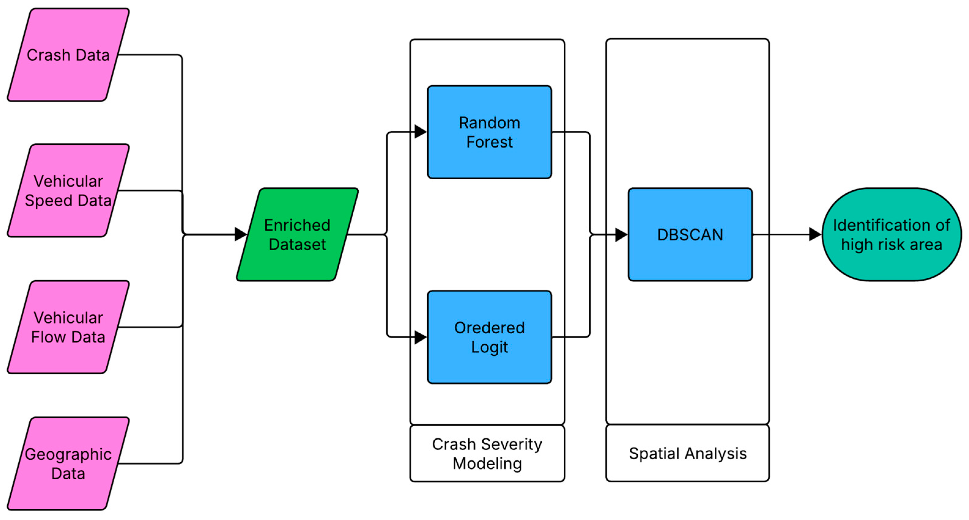
This section details the overall methodology adopted in this paper, as well as the dataset and the implemented models. As shown in Figure 1 below, data collected from various sources, ranging from crash data to geographic data, are combined through data fusion. The enriched dataset is characterized by greater complexity and more informative content than typical crash datasets. Following data collection and pre-processing, two different models are calibrated: Random Forest and Ordered Logit. These models belong to two distinctive fields, and, in particular, Machine Learning and Econometrics, respectively. Both approaches are employed to classify cyclist crash injury severity (i.e., the probability of a Fatal vs. Injured vs. Uninjured Outcome). A key element of this methodology is the analysis of prediction residuals of the two distinctive severity models. It can be assumed and hypothesized that misclassified observations, which are the prediction errors of the model, result from “latent” or “unobserved” spatial variables that the model fails to capture. Consequently, a spatial analysis with the DBSCAN is conducted on these misclassified georeferenced observations, aiming to detect spatial clusters and latent contributing and unexplained factors to identify high-risk areas.

3.1. Dataset and Variables Description

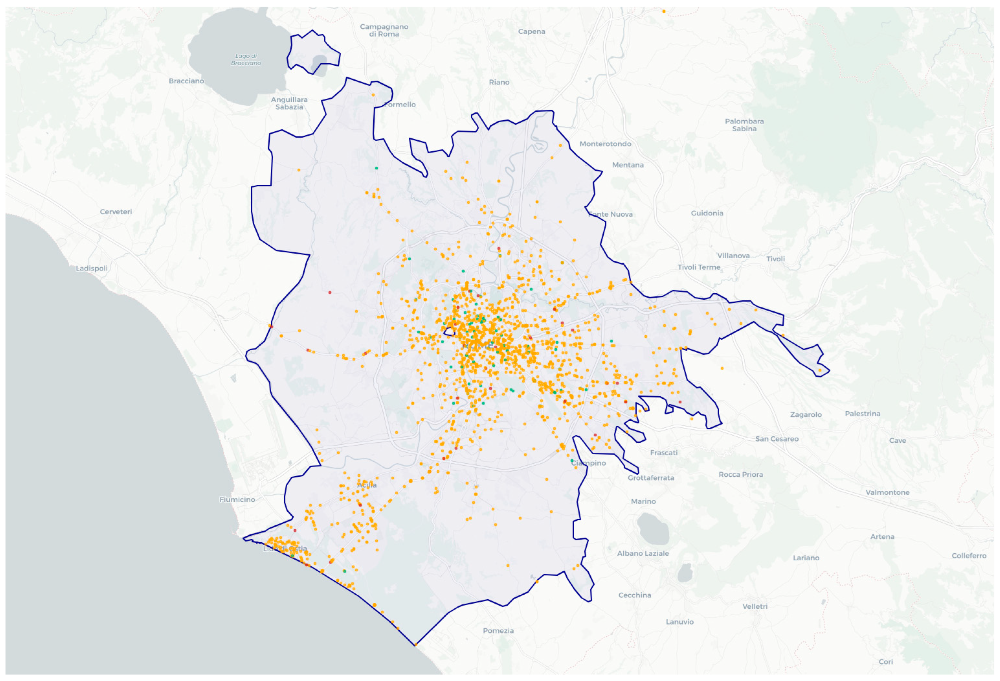
Road safety, as suggested by the literature and the European and global plans, is crucial in defining design strategies for the future and reaching environmental and safety objectives. The major issues are related to urban environments, especially metropolitan cities worldwide. For this reason, this study focuses on eight years (2013–2020) of available cyclist crashes in the city of Rome, Italy (see Figure 2).

The original dataset used for the study is provided by the Italian Institute of Statistics (ISTAT) [25]. The dataset collects crash events for each type of road user, but the focus in this research will be on cyclist crashes, which are among the most exposed to risks (see

Table 1. Variable description and organization after the data fusion phase.

Macro Category	Variable	Categories
Temporal Factors	Day of the Week	Weekday, Weekend
	Time of the Day	Day (07–15), Afternoon (16–19), Evening (20–23), Night (24–06)
Environmental and Infrastructural	Location Context	Urban, Not Urban
	Road Type	One-way Carriageway, Two-way Carriageway, Two Carriageways, More than Two Carriageways
	Road Stretch	Road (Link), Intersection
	Weather Conditions	Clear Weather, Adverse Weather
Traffic and Network Data *	Vehicular Speed *	0–30 km/h, 30–50 km/h, >50 km/h
	Vehicular Flow *	<500 veh/h, 500–1000 veh/h, >1000 veh/h
Cyclist Characteristics	Gender	Female, Male
	Age	Young (Under 25), Adults (25–65), Elderly (Over 65)
Collision Partner	Interaction Type	No Collision Partner;
	(Vehicle × Age × Gender)	Car: Young (F/M), Adult (F/M), Elderly (F/M), N.A. (F/M);
		Heavy Vehicle: Young (M), Adult (F/M), Elderly (M), N.A. (F/M);
		Powered Two-Wheeler: Young (F/M), Adult (F/M), Elderly (M), N.A. (F/M);
		Other Micro-mobility: Young (F/M), Adult (M), Elderly (F), N.A. (F/M/Unknown)
Land Use and Facilities (POIs) *	Food Service Establishments *	No, Yes
	Commercial Activities *	No, Yes
	Educational Facilities *	No, Yes
	Transport Facilities *	No, Yes
	Cyclist Facilities *	No, Yes
	Pedestrian Facilities *	No, Yes

* These variables are added to the original dataset via data fusion.

for a brief description of the variable in the dataset). The whole dataset contains, before the prepossessing phase, 2139 cyclist crashes, of which 1865 are georeferenced. After the preliminary cleaning stages, the resulting dataset contains 2093 observations, and 1826 of them are georeferenced: 32 (1.7%) are Fatal, 1705 (93.4%) are Injured, and 89 (4.9%) are Uninjured. As shown in

Table A1. Brief descriptive statistical analysis to detail variables and dataset structure.

Variable	Fatal [%]	Injured [%]	Uninjured [%]	VIF [-]
Weekday	1.7	93	5.3	Ref.
Weekend	1.9	94.6	3.5	1.09
Afternoon_16_19	1.2	92.6	6.2	Ref.
Day_07_15	2	93.4	4.6	1.45
Evening_20_23	1	95.9	3.1	1.4
Night_24_06	2.7	91.9	5.4	1.22
Not_Urban	4.8	92.9	2.4	Ref.
Urban	1.5	93.4	5.1	1.24
More_than_two_carriageways	4.9	87.7	7.4	Ref.
One_way_carriageway	0.7	94.9	4.3	2.93
Two_carriageways	2.9	94.4	2.7	2.86
Two_way_carriageway	1.1	93.2	5.7	3.67
Adverse_Weather	1.1	95.7	3.2	Ref.
Clear_Weather	1.8	93.2	5	1.03
Cyclist_Adults_25_65	1.3	94.2	4.5	Ref.
Cyclist_Elderly_over65	5.9	92.2	2	Ref.
Cyclist_Young_Under_25	0	90.4	9.6	Ref.
Female	1.6	94.7	3.8	Ref.
Male	1.8	93.1	5.1	1.07
Intersection	1.4	94.8	3.8	Ref.
Road	1.9	92.6	5.5	1.14
Car_Adults_25_65_Female	0	100	0	Ref.
Car_Adults_25_65_Male	1.6	98	0.4	2.21
Car_Elderly_over65_Female	0	100	0	1.16
Car_Elderly_over65_Male	1.2	98.8	0	1.52
Car_Not_applicable_Female	0	100	0	1.05
Car_Not_applicable_Male	6.2	93.8	0	1.06
Car_Young_Under_25_Female	0	100	0	1.11
Car_Young_Under_25_Male	3.4	96.6	0	1.22
Heavy_vehicle_Adults_25_65_Female	0	100	0	1.02
Heavy_vehicle_Adults_25_65_Male	10.8	88	1.2	1.3
Heavy_vehicle_Elderly_over65_Male	0	100	0	1.02
Heavy_vehicle_Not_applicable_Female	0	100	0	1.01
Heavy_vehicle_Not_applicable_Male	33.3	66.7	0	1.02
Heavy_vehicle_Young_Under_25_Male	16.7	83.3	0	1.03
No_Collision_Partner	0.5	89.9	9.6	2.16
Other_micro_Adults_25_65_Male	0	85.7	14.3	1.07
Other_micro_Elderly_over65_Female	0	100	0	1.05
Other_micro_Not_applicable_Female	0	66.7	33.3	1.03
Other_micro_Not_applicable_Male	14.3	64.3	21.4	1.08
Other_micro_Not_applicable_Unknown	2.9	97.1	0	1.13
Other_micro_Young_Under_25_Female	0	100	0	1.02
Other_micro_Young_Under_25_Male	0	100	0	1.04
Powered_two_wheeler_Adults_25_65_Female	0	60	40	1.06
Powered_two_wheeler_Adults_25_65_Male	1.7	74.4	23.9	1.42
Powered_two_wheeler_Elderly_over65_Male	11.1	77.8	11.1	1.05
Powered_two_wheeler_Not_applicable_Female	0	100	0	1.01
Powered_two_wheeler_Not_applicable_Male	0	100	0	1.01
Powered_two_wheeler_Young_Under_25_Female	0	75	25	1.03
Powered_two_wheeler_Young_Under_25_Male	0	78.3	21.7	1.1
Vehicular_Speed > 50 *	3.4	91.7	4.9	Ref.
Vehicular_Speed_0_30 *	1.4	94.8	3.9	1.58
Vehicular_Speed_30_50 *	0.7	93.2	6.1	1.55
Vehicular_Flow < 500 *	1.2	94.9	3.9	Ref.
Vehicular_Flow > 1000 *	2.8	89.8	7.4	1.35
Vehicular_Flow_500_1000 *	2	93.5	4.5	1.21
Food_service_establishments_No *	2.2	93.8	4.1	Ref.
Food_service_establishments_Yes *	0.6	92.3	7.1	1.31
Commercial_activities_No *	1.8	93.5	4.8	Ref.
Commercial_activities_Yes *	1.7	92.2	6.1	1.19
Educational_Facilities_No *	1.8	93.5	4.7	Ref.
Educational_facilities_Yes *	0	89.7	10.3	Ref.
Transport_Facilities_No *	2	93.4	4.6	Ref.
Transport_Facilities_Yes *	1.2	93.2	5.6	1.17
Cyclist_Facilities_No *	1.9	93.7	4.3	Ref.
Cyclist_Facilities_Yes *	0.7	91.4	7.9	1.12
Pedestrian_Facilities_No *	3.4	92.8	3.8	Ref.
Pedestrian_Facilities_Yes *	1.2	93.6	5.2	1.4

* These variables are added to the original dataset via data fusion.

(Appendix A.1), which provides a brief description of the variables and dataset structure, crashes are generally more likely to occur on weekdays than on weekends, and during morning hours rather than at night. As can be observed, the vast majority of crashes occur within urban areas. From the description, it also emerges that interaction between motorized and non-motorized flows may play a key role: two-way carriageways and two carriageways are characterized by a high probability that a cycle crash may lead to a serious or fatal injury. These interactions are badly correlated to cyclist outcomes, and single-lane carriageways seem to lead to a lower probability of fatal crashes. It is worth noting that in half of the fatal cyclist crashes recorded, the road users who cause the crash are male adults (aged between 25 and 65 years) who drive a car or a heavy vehicle. Also, traffic-related features show this particular trend: 18 cyclist crashes over 32 are characterized by the speed of the vehicle greater than 50 km/h, while there is no significant variation across high or low traffic flows. Cyclists under 25 years, according to this brief exploratory analysis, seem not prone to fatal injuries after crashes, compared to older ones. The last aspect that emerges from Table A1 and from a brief description of variable and dataset is that in the absence of food service establishments (bars, cafés, and restaurants), commercial activities, educational facilities (schools and universities), transport facilities (bus stops, metro and railway stations, and parking), and cyclist facilities (cycleways), the number of crashes is higher compared to less isolated environments.

To ensure that the parameter estimates were not biased by multicollinearity among the independent variables, the Variance Inflation Factor (VIF) was calculated. All variables exhibited VIF values < 3.67, indicating no significant multicollinearity issues. This statistical analysis is reported in Table A1 (see Appendix A.1).

3.2. Random Forest and Variable Importance

It has been demonstrated that Random Forest (RF) has good prediction performances [26,27] compared to other classification and regression models. In addition to that, this model is correlated with two byproducts that are out-of-bag estimates of generalization error [28,29] and variable importance measures [26,29,30].

Tree-Based Methods (TBM) are designed to model non-linear relationships and to classify and regress observations according to some stratification rules of the independent variable by building a partition of the original data into sub-groups [31]. These regions are known as terminal nodes or leaves, and the nodes not in the leaves are called internal nodes. The branches that connect the leaves with the internal nodes define a hierarchical structure. The length of these branches is proportional to the deviance of the nodes. How to build a tree? First of all, the predictor space is divided to create nonoverlapping regions; then, for each region, the same prediction is performed for every observation. The RSS is used as a benchmark to assess the performance of the tree. These trees are built recursively and hierarchically: at each step, the best split is made according to some measures of homogeneity of the resulting split, and is made at that step without looking ahead, with a myopic way to proceed [32]. This way also leads to the problem of correlation among trees. Each time a split is made, the number of final leaves (and so the dimensionality of the tree) increases by one. It is essential to include a stopping rule that can be based, for instance, on the final number of leaves needed on the number of observations in the final nodes, or on the value of the resulting degree of purity of the nodes. By increasing the number of leaves, the bias decreases, the complexity and the variance increase: fitting a too-complex tree might have poor prediction accuracy. Also, a high degree of interpretability leads to poor prediction accuracy. In general, a simple tree with few splits provides poor predictions because the functional form is very rigid and tends to predict the same value for a high number of observations. To increase the prediction accuracy, the tree must be more complex, but prediction increases up to some point. One stopping rule is the pruning function, which is a function that takes into account the RSS and penalty function to prevent the problem of overfitting. Regarding the classification tree, this is very similar to the regression tree: the main difference is that the performance of the model is not measured in terms of Mean Squared Error (MSE) but rather in terms of misclassification error rate, which is proportional to the fraction of training observations in a given leaf that do not belong to the most common class. Other measures of misclassification are the Gini index and the Entropy. TBMs are quite easy to obtain and use a quite intuitive structure because there is no functional form to estimate, but a division of data according to the rule of the dependent variable. They also provide good interpretability of the results. The main drawback is that TBMs do not have the same level of prediction accuracy as other methods and are not very robust because when there is a change in the data references, they do not provide good predictions.

Tree-Based Methods include Decision Tree Models (DT), which differ from regression trees because they are used to predict a qualitative variable. RSS cannot be used as a criterion for splitting; instead, the Classification Error Rate (CER) is used. Gini index (GI) is also used instead of CER due to its sensitivity to measure total variance across the K classes [33]. They were first introduced in 1983 by Breiman et al. [29]; the aim is to split the problem search space into subsets and build the tree in a top-down way using the training set.

Decision Trees suffer from a high variance, and that means that in the splitting phase of the training and the test set, a DT could give different output performance according to how the splitting is made. In the field of TBM, reducing the variance, bootstrap aggregation, or Bagging, can be used to improve the DT’s high variance problem by taking samples from the training dataset. Random Forest (RF), unlike Bagging, works in a way to decorrelate the trees generated. If there is a strong predictor in the dataset, Bagging considers the predictors that play an important role. In RF, only a subset of predictors is considered [34]. The RF method collects classification from each DT and then combines them according to some rules (majority vote or confidence vote strategy), with the idea that using a combination of several learning models improves the prediction accuracy of the considered model [35]. By working in this way with trees that are bootstrapped and random features used to generate trees, the different trees are not correlated, and the problem of overfitting is avoided [36]. According to Yan et al. [32], the RF algorithm can be described as follows:

• k bootstrapped training sets are generated from the original dataset;
• Each tree is trained on a single k-bootstrapped dataset, and the nodes are split by a randomly selected feature: this step is iterated k times to obtain k trees;
• Each trained tree gives its prediction accuracy: the final model is determined by the majority voting or confidence vote strategy from all the k models.

The first scientist to propose RF was Tim Kam Ho in 1995 [33], but a few years later (2001), it was improved by Leo Breiman [29].

In the variable importance (VIP) method, VIP is evaluated as a mean decrease in accuracy by using out-of-bag observations (OOB) (L_b,oob), because the tree grows from a bootstrapped sample (L_b) of the original training sample (L). The procedure to evaluate VIP can be summarized as follows, according to Archer et al. [37]:

• For bootstrap sample b = 1,…, B, it is possible to identify the OOB observations, L_b,oob = L/L_b;
• Predict class membership for L_b,oob using Tb, and sum the number of times the tree predicts the correct class;
• For independent variables j = 1,…,p:

(a)

Permute the values of the independent variable x_j in L_b,oob.

(b)

Use Tb to predict class membership for L_b,oob using the permuted x_j values; sum the number of times the tree predicts the correct class for the L_b,oob observations.

(c)

Subtract the number of votes for the correct class in the permuted OOB data from the number of votes for the correct class in the OOB data.

The average difference in the accuracy of the OOB and permuted OOB observations over the B trees is the variable importance measure for x_j.

The whole dataset has been split into a training set (which includes 70% of observations) and a test set (the remaining 30%). Due to the high-class imbalances in road crash datasets, a Stratified Hold-Out random split (and not temporal or spatial) has been used. This approach ensures that the proportion among classes in the original dataset is also in the training and test sets. Additionally, in the training and test phase, variables such as geographical coordinates and road names have been removed to avoid spatial leakage.

3.3. Ordered Logistic Regression

The second crash injury severity model calibrated and implemented in this work is the Ordered Logistic Regression (OLR). Econometric Models, also known as Discrete Choice Models, are explainable and interpretable models that have been extensively used to predict crash injury severity. A first classification of these models could be made on the unordered or ordered formulations of the dependent variable [38]. Usually, crash severity could be divided into two or more classes (in this particular case, Fatal, Injured, and Uninjured) that follow an increased level of registered damages. In this case, the response variable shows an ordered nature, and the model (OLR) can take into account this aspect. If the response or dependent variable does not follow this particular structure and the variables do not follow a particular order, Binary Logistic Regression (BLR) or Multinomial Logistic Regression (MLR) could be used instead [39]. Another point to discriminate models is based instead on the number of classes to be predicted. OLR does not follow this logic; it only requires that the dependent variable shows an inner order, whereas BLR and MLR are used to predict two or more classes, respectively. Before moving to the OLR description, it can be useful to highlight the structure of the simplest model. BLR is an Econometric Model that is usually implemented for classification tasks [40]. It is worth noting that, unless Linear Regression, Logit Models are implemented for classification [41]. Usually, the outcome Y can be described as follows (Equation (1)):

$$Y=\left\{\begin{array}{c}1 if the phenomenon occurs\\ 0 if the phenomenon does not occur\end{array}\right.$$

(1)

In a binary problem, Y could assume the value 1 if the cyclists are dead, 0 if only Injured or Uninjured.

BLR, despite RF and Machine Learning Algorithms, is used to make inferences due to its high interpretability. With this model, it is possible to understand the relationships among independent and dependent categorical variables [42]. The structure of BLR could be expressed in the following equation (Equation (2)), which gives the probability that the event Y = 1 happens, given the vector X of independent variables:

$$p(Y=1\mid X)={\displaystyle \frac{e^{{\beta }_0+\sum {\beta }_i{X}_i}}{1+e^{{\beta }_0+\sum {\beta }_i{X}_i}}}$$

(2)

where p(X) is the predicted probability; x_i are the independent variables or features; β₀…β_i are the estimates or coefficients of the model. The model in Equation (1) only allows for two classes of the response or dependent variable. Although more complex Machine Learning Algorithms such as RF exist, BLR or MLR offer clearer interpretability. Another advantage is its straightforward structure, which makes it easier for end users to understand. On the contrary, Econometric Models may produce unstable results due to the large amount of data, a common feature when road crash data are used [43]. Reducing the number of variables, for example, by applying a Machine Learning-based feature selection algorithm, could be a winning strategy.

By extracting the logarithm from the model in Equation (2), the Odds Ratio (OR) that represents the relative probability that a phenomenon occurs given a baseline condition could be evaluated (Equation (3)):

$$OR={\displaystyle \frac{p(Y=1\mid X)}{1-p(Y=1\mid X)}}={\beta }_0+\sum {\beta }_i{X}_i$$

(3)

To handle the ordered nature of cyclist injury severity [44], OLR overcomes the main limitation of BLR and MLR regarding the loss of ordering information for the dependent variable [45,46]. The main assumption underlying an OLR is that there exists an unobserved continuous variable (also called latent), which, in this case, represents the propensity of a given individual within the population to use a particular mode of transportation. For each individual i, with I = 1…N, there exists a latent variable Y_i* that can be expressed as (Equation (4)) [47]:

$${\mathrm{Y}}_{\mathrm{i}}^{\mathrm{*}}={\mathrm{x}}_{\mathrm{i}}\prime \beta \mathrm{ }+{\epsilon }_{\mathrm{i}}$$

(4)

where

• ${\mathrm{Y}}_{\mathrm{i}}^{\mathrm{*}}$ is the propensity or latent (unobserved) variable;
• ${\mathrm{x}}_{\mathrm{i}}$ is the vector of observed independent variables;
• β is the vector of coefficients to be calibrated and estimated;
• ${\epsilon }_{\mathrm{i}}$ is the error term, which follows a standard logistic distribution. If it followed a normal distribution, the model would instead be referred to as an Ordered Probit.

If the number of response options or categories is J, the model estimates J − 1 thresholds, also called τ₁…τ_J−1, ordered in increasing value [48]. If Y is the observed response or category (in this case, 1, 2, and 3), the relationship between the unobserved and observed variable can be described as (Equation (5)):

$$Y_i=j\hspace{1em}\mathrm{se} \hspace{1em}{\tau }_{j-1}<Y_i^{*}\le {\tau }_j$$

(5)

Since the goal is to calculate the probability that an individual i chooses category j, the cumulative distribution function (CDF) of the logistic distribution, F(z), can be used (Equation (6)):

$$F\left(z\right)={\displaystyle \frac{e^z}{1+e^z}}={\displaystyle \frac{1}{1+e^{-z}}}$$

(6)

The model classifies the choice of a user i into category j if and only if the probability associated with the latent utility falls between the two thresholds that define that category:

$$P\left(Y_i=j\right)=P\left({\tau }_{j-1}<Y_i^{*}\le {\tau }_j\right)=P\left({\tau }_{j-1}<x_i^{\prime }\beta +{\epsilon }_i\le {\tau }_j\right)=P\left({\tau }_{j-1}-x_i^{\prime }\beta <{\epsilon }_i\le {\tau }_j-x_i^{\prime }\beta \right)$$

(7)

By combining the previous expression (Equation (7)) with the definition of the CDF, also defined as F(z) (Equation (6)), the probability formula is obtained (Equation (8)):

$$P\left(Y_i=j\right)=F\left({\tau }_j-x_i^{\prime }\beta \right)-F\left({\tau }_{j-1}-x_i^{\prime }\beta \right)$$

(8)

Due to high class imbalances in the dataset, to overcome this limitation, different weights are given to observations of the three classes, according to Equation (9) [49]:

$$w_j={\displaystyle \frac{N}{c\times N_j}}$$

(9)

where j is the specific class or severity level (Uninjured = 1, Injured = 2, Fatal = 3); w_j is the weight applied to observation belonging to class j; c is the total number of classes (in this case 3); N is the total number of observations in the dataset; N_j is the number of observations belonging to class j. Unlike what was previously performed with RF, dataset balancing techniques such as SMOTE were not used with OLR. The reason is mainly that in Econometric Models, adding synthetic observations would have reduced the standard error and thus led to biased p-values. On the other hand, SMOTE was chosen for the RF because the addition of synthetic observations to unbalance the minority class allows for finding the rules and the decision boundaries for classifying the classes.

3.4. DBSCAN

The Density-Based Spatial Clustering of Applications with Noise (DBSCAN) is a common and widely used spatial clustering technique based on the assumption that regions can identify a cluster with a high density of points or observations [50]. Unlike clustering methods such as K-Means [51], DBSCAN defines clusters as high-density areas separated by regions of lower density. In addition, it does not use some predefined shapes, but it can follow road shapes. It is worth noting and mentioning that DBSCAN is applied to misclassified observations from the previous models (RF and OLR). The spatial model can handle outliers, allowing isolated misclassification errors (noise) to be filtered out and focusing the analysis only on systematic concentrations of errors (clusters), which indicate local latent variables not captured by both LR and OLR.

The main parameters on which the algorithm is based are the radius ε and MinPts, that is, the minimum number of points or observations needed for clustering individuation [52,53,54,55]. The points and the observations that fall in a cluster could be classified in three ways. The first are defined as Core points, which have a sufficient number of neighbors. Then the Border points, which are near the border of the cluster, and finally the Noise points, which could not be included in a cluster.

If D is a dataset of observations with coordinates defined as $\left(x, y\right)$, and p and q are two points distant by a quantity dist(p, q), the sample of points that are distant less than ε could be described as follows:

$${\mathrm{N}}_{\epsilon }\left(\mathrm{p}\right)\mathrm{ }=\mathrm{ }\{\mathrm{ }\mathrm{q}\mathrm{ }\in \mathrm{ }\mathrm{D}\mathrm{ }\mid \mathrm{ }\mathrm{d}\mathrm{i}\mathrm{s}\mathrm{t}\left(\mathrm{p},\mathrm{ }\mathrm{q}\right)\mathrm{ }\le \mathrm{ }\epsilon \mathrm{ }\}$$

(10)

A point p is a Core point if the number of neighbor points is more than or equal to the minimum number of points or observations needed for clustering individuation:

$$\left|{\mathrm{N}}_{\epsilon }\left(\mathrm{p}\right)\right|\mathrm{ }\ge \mathrm{ }\mathrm{M}\mathrm{i}\mathrm{n}\mathrm{P}\mathrm{t}\mathrm{s}$$

(11)

If this condition is met, a new cluster is identified.

4. Results

4.1. Crash Severity Injury Model Performances

In this subsection, the first results in terms of model performances are shown. As mentioned in Section 3 on the methodology aspect, the two crash severity injury models developed are RF and OLR. These models belong to two different fields, with RF and, in general, Machine Learning Algorithms being often implemented to make predictions, while OLR and Econometric Models are used to make statistical inference. In order to make a comparison among models, some performance metrics are needed: since OLR and RF are used for a classification task, Precision, Recall, and F1 score are chosen as main comparison metrics and evaluated for each class. Model results in terms of main statistics are reported in

Table 2. The main performance metrics of OLR.

Class	Precision	Recall	F1-Score	Balanced Accuracy	McFadden (Pseudo R2)
Uninjured	0.84	0.16	0.28	0.4033	0.4695
Injured	0.60	0.98	0.75
Fatal	0.78	0.07	0.14
Macro Average	0.74	0.41	0.39

and

Table 3. The main performance metrics of RF.

Class	Precision	Recall	F1-Score	Balanced Accuracy
Uninjured	0.14	0.11	0.13	0.4266
Injured	0.94	0.95	0.95
Fatal	0.20	0.22	0.21
Macro Average	0.43	0.43	0.43

.

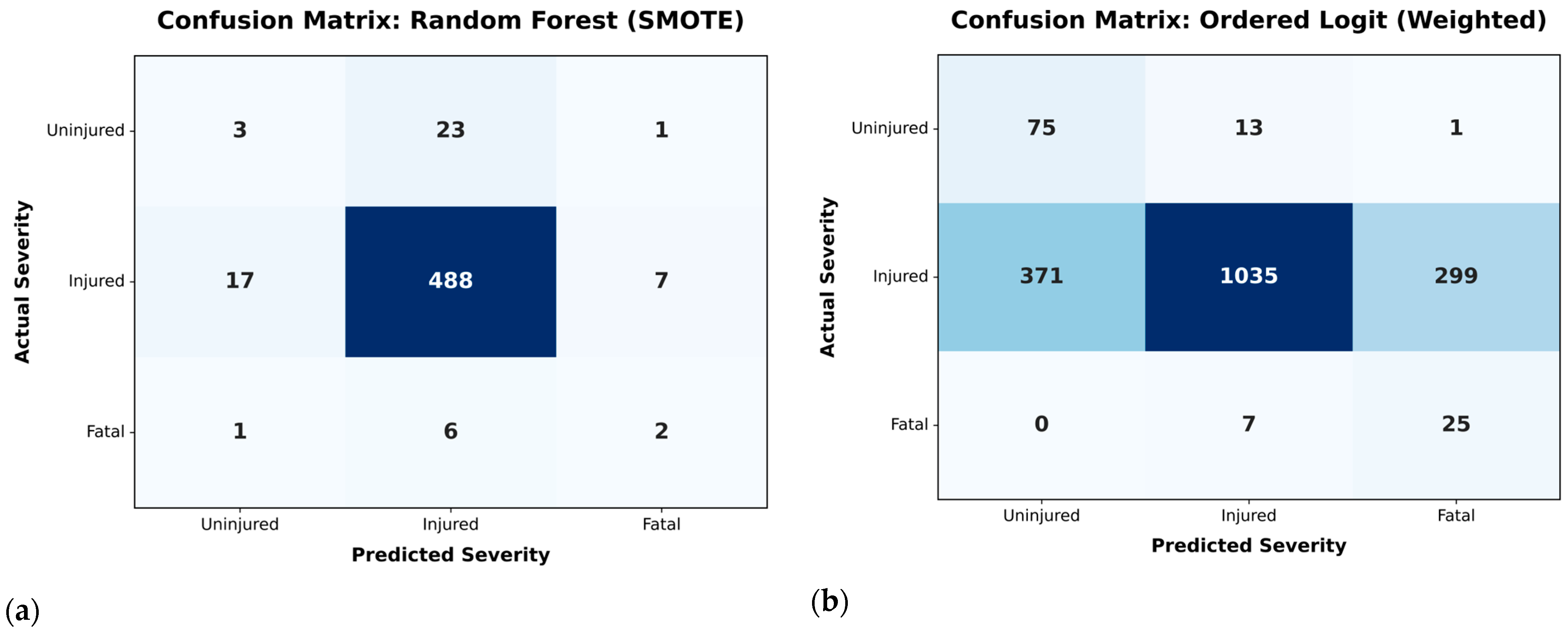
Starting from the Uninjured class, OLR shows a good Precision (0.84) but a low Recall (0.16). This trend highlights how OLR, when predicting a crash with an uninjured cyclist, has a high probability that the forecast is correct. But with the low value of Recall on the Uninjured class, and a high Recall on the Injured class, the models overestimate the crash severity by predicting more injuries. The RF’s Precision, Recall, and F1 score for the Uninjured class show that the models cannot distinguish between an uninjured and an injured cyclist. In the Injured class, RF shows high predictive performance with Precision (0.94), Recall (0.95), and F1 score (0.95). This means that RF can predict with high accuracy the outcome of an observation. OLR, as well as RF, is characterized by a high value of Recall (0.98), but a lower level of Precision (0.60); this means that again, OLR overestimates the injury severity of some observations. It is worth remembering that the dataset on which models are calibrated is skewed towards the Injury class, and to overcome class imbalance, for RF calibration, oversampling techniques such as SMOTE [56] are implemented, while for OLR, only some weights (see Equation 9) are applied. For the Fatal class, both models show good performance in terms of F1 score (0.21 and 0.14 for RF and OLR, respectively) in relation to the strong imbalances in the dataset. With a higher Recall than OLR, RF performs better in identifying fatal crashes. In terms of Balanced Accuracy (a metric commonly used for serious imbalanced problems), both models show almost the same performance.

By comparing the Confusion Matrices (CM) shown in Figure 3, it is possible to observe not only the different structure between the two approaches but also how models classify observations. As can be seen in Figure 3a (note that the CM on the test set is reported), the RF correctly identifies two out of nine actual fatal crashes (22%). Regarding precision, the model predicts several fatal crashes that turn out to be injuries, showing cautionary behavior. The weighted OLR (see Figure 3b) shows high sensitivity, correctly classifying 25 out of 32 actual fatalities (78%). This high sensitivity also results in a high false-positive rate because 299 injuries have been classified as fatalities. Although this could be seen as a deficiency of the model, on the other hand, in the context of road safety, this could be an advantage in identifying high-risk scenarios. This trend observed in OLR confirms that the use of weight in OLR improves model prediction towards the fatal class. In conclusion, OLR can better explain the crash risk factor contributions than RF (due to the interpretable nature of Econometric Models), while RF provides superior prediction performance.

4.2. Contributing Risk and Mitigation Factors Related to Cyclists’ Injury Severity

For the OLR, the McFadden or Pseudo-R2 (0.4695) is also evaluated, indicating a good fit and an accurate explanation of contributing factors related to cyclist injury severity. Due to its linear nature and underlying assumptions, its explanatory capabilities surpass its classification capabilities. On the contrary, RF, like all Machine Learning Algorithms, works like a black box and suffers from low interpretability. Combining these two different methodologies could be a fair compromise.

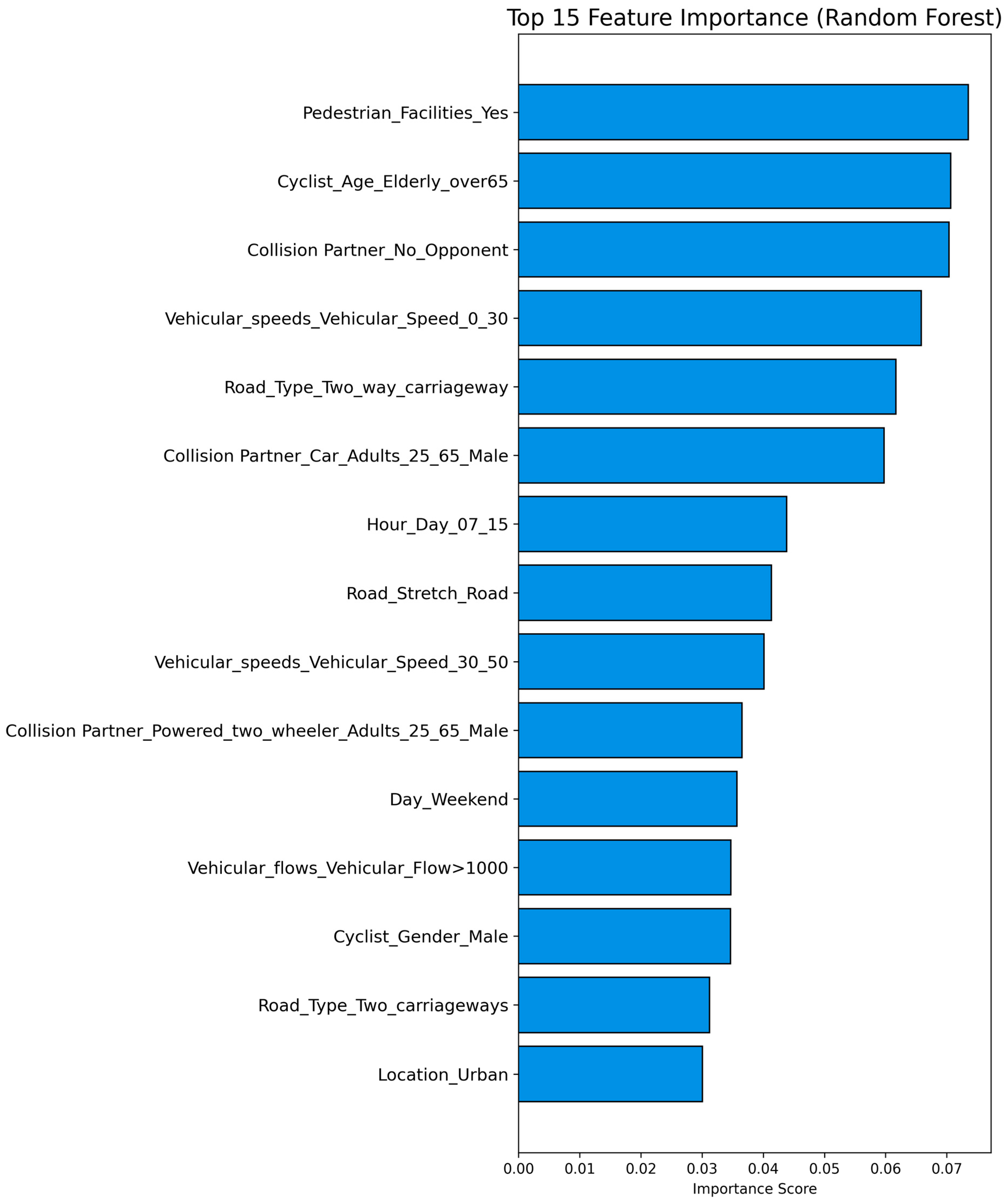
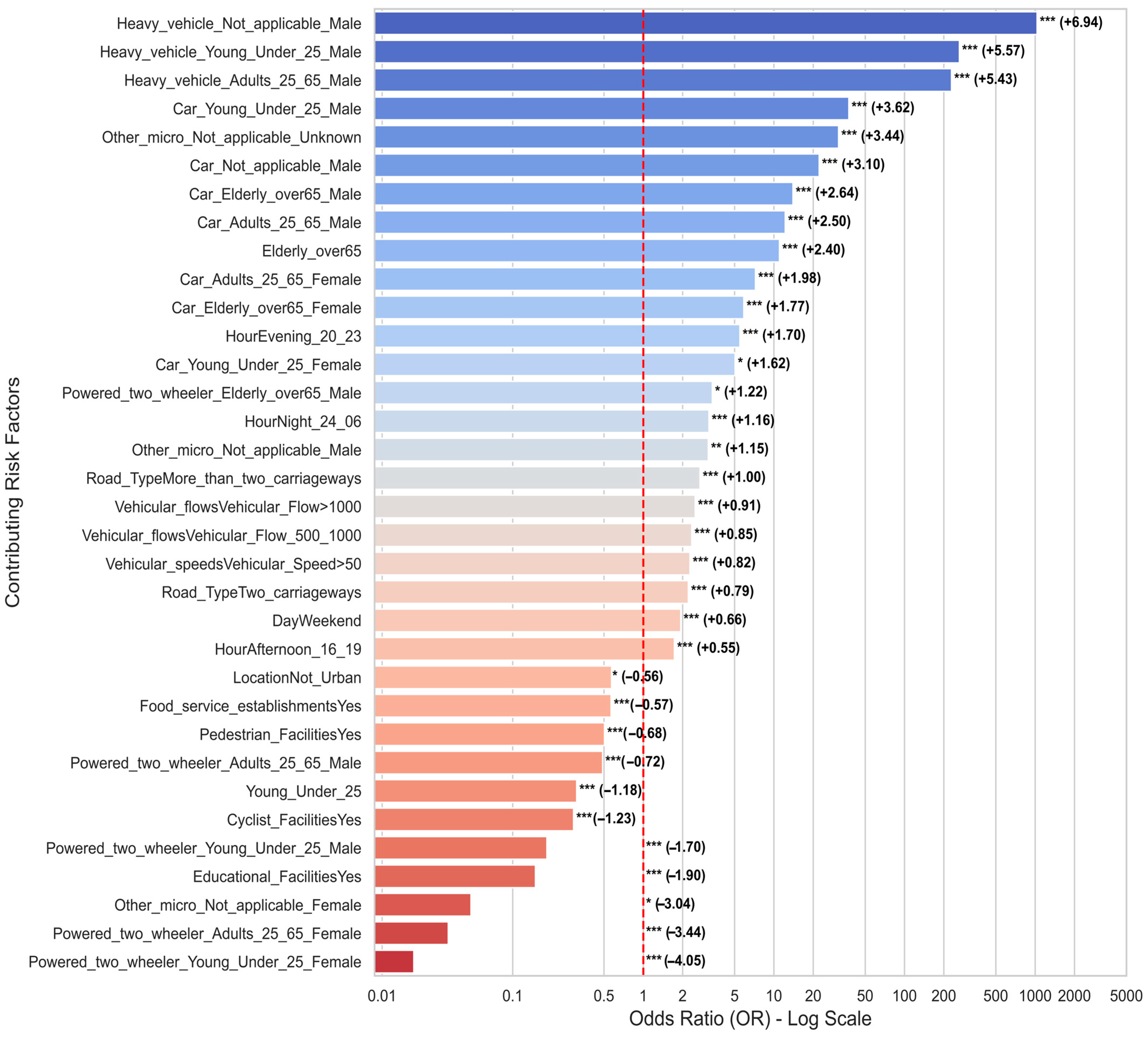
As shown in Figure 4 and Figure 5, both RF and OLR can be used to model variable contribution. Starting from Figure 4 and the RF results, contributing factors are ranked according to the Importance Score and, to improve readability, only the first 15 variables selected as relevant from the model are reported. In Figure 5, instead, the results from the OLR are reported and, in particular, the most significant variable, in descending order, according to the Odds Ratio (OR).

A preliminary comparison of the results from the two models reveals that they agree. For example, risk factors identified by both models include “Pedestrian_FacilitiesYes” (indicating the presence of pedestrian infrastructure near the crash site), “Cyclist_Age_Elderly_over65” (cyclist age over 65), “Collision_Partner_Car_Adults_25_65_Male” (cyclist hit by a car driven by a male aged 25–65), “Collision_Partner_Powered_two_wheeler_Adults_25_65_Male” (cyclist hit by a powered two-wheeler driven by a male aged 25–65), “Day_Weekend” (indicating the crash occurred on Saturday or Sunday), “Vehicular_Flow > 1000” (indicating a vehicular flow greater than 1000 vehicles/hour), and “Road_Type_Two_carriageways” (indicating the road type is a two-carriageway). Other variables considered important by the Random Forest (RF) model are used as baseline values in OLR and are consequently not present in Figure 5. The only variable considered a risk factor by the RF and not by OLR is “Vehicular_Speed_30_50”. As can be inferred from Figure 4, the Variable Importance Analysis with RF alone provides indications of which risk factors have a high Importance Score, but not how these factors specifically impact the severity of the cyclist crash. For example, the model identifies “Pedestrian_FacilitiesYes” as significant, but it is not immediately clear whether the presence of pedestrian facilities correlates with a lower or a greater risk of fatal outcome for a cyclist involved in a crash.

The OLR model, on the other hand, provides a more immediate and interpretable explanation of the phenomenon. In Figure 5, the most significant variables identified by the model are reported, sorted in descending order by Odds Ratio (OR). A dashed red line is also plotted on the graph corresponding to OR = 1. As stated in the methodology section, and specifically in Section 3.2, the OR indicates how much the probability (in this case, the odds of a cyclist being killed) increases in relative terms, compared to a baseline value (which is chosen during model calibration and is reported in Table A1 in the Appendix A.1). This means that variables presenting an OR > 1 can be assimilated to risk factors, while variables with OR < 1 can be considered mitigation factors. What emerges from Figure 5, compared to Figure 4, is that OLR, relative to RF, is able to provide a more detailed framework that allows for inference, and also enables a full understanding of the role of individual variables in the cycling crash phenomenon, despite having lower performance than the RF. Since the OR is a ratio, using the first variable in Figure 5 as an example, if a cyclist is hit by a heavy vehicle driven by an unspecified male user, the odds of being involved in a fatal crash are about 1000 times higher compared to those in which a cyclist crashes alone or collides with an obstacle (the baseline). It is worth recalling that the values in parentheses represent the model’s estimates: risk factors present positive estimates, while mitigation factors present negative estimates.

Starting from the risk factors, these can be grouped into five categories as emerges from Figure 5: Collision Partner, Cyclist Age, Hour of the Day, Road Type, Day, and Traffic-Related Variables. Among the top positions occupied by variables with a considerable OR are specific Collision Partners, particularly users driving heavy vehicles, predominantly males under 65 years of age. This variable presents a high OR, and this is indicative of quasi-complete separation in the dataset (which occurs when a predictor perfectly predicts the outcome due to sparse data or small sample sizes within a specific class), which is physically consistent with the nature of bicycle-heavy vehicle collisions (due to different masses and speeds). The baseline category corresponds to a single-vehicle crash (e.g., a cyclist falling alone). Comparing the biomechanical impact of falling alone versus a collision with a heavy vehicle, it is physically consistent that the OR of a severe/fatal outcome increases dramatically. Despite this statistical criticality, the model nevertheless remains stable, and this stability is ensured by a comparison between the estimates, standard error, and Confidence Interval (CI) of the model variables (see

Table A2. Description of the OLR model.

Variable	Baseline	Estimate	Std_Error	p_Value	OR	95% CI
Day_Weekend	Weekday	0.6609	0.1515	0.00001 ***	1.9365	[1.44–2.61]
Hour_Afternoon_16_19	Morning_07_15	0.5464	0.1433	0.00014 ***	1.727	[1.30–2.29]
Hour_Evening_20_23	‘’	1.7018	0.2337	0 ***	5.4838	[3.47–8.67]
Hour_Night_24_06	‘’	1.1574	0.2958	0.00009 ***	3.1815	[1.78–5.68]
Location_Not_Urban	Urban	−0.5597	0.2627	0.03308 *	0.5714	[0.34–0.96]
Road_Type_More_than_two_carriageways	Two-way Carriageway	0.9993	0.2003	0 ***	2.7162	[1.83–4.02]
Road_Type_One_way_carriageway	‘’	−0.1087	0.1689	0.51985	0.897	[0.64–1.25]
Road_Type_Two_carriageways	‘’	0.7941	0.1615	0 ***	2.2124	[1.61–3.04]
Weather_Adverse_Weather	Clear Weather	0.0637	0.2836	0.82217	1.0658	[0.61–1.86]
Cyclist_Age_Elderly_over65	Adults 25–65 years	2.4003	0.1811	0 ***	11.0269	[7.73–15.73]
Cyclist_Age_Young_Under_25	‘’	−1.176	0.181	0 ***	0.3085	[0.22–0.44]
Cyclist_Gender_Female	Male	0.2726	0.1646	0.09775	1.3134	[0.95–1.81]
Road_Stretch_Intersection	Road	−0.1742	0.1439	0.22584	0.8401	[0.63–1.11]
Collision_Partner_Car_Adults_25_65_Female	No Collision_Partner	1.9767	0.2515	0 ***	7.2188	[4.41–11.82]
Collision_Partner_Car_Adults_25_65_Male	‘’	2.5022	0.1923	0 ***	12.2096	[8.38–17.80]
Collision_Partner_Car_Elderly_over65_Female	‘’	1.7714	0.5222	0.00069 ***	5.8793	[2.11–16.36]
Collision_Partner_Car_Elderly_over65_Male	‘’	2.6386	0.2697	0 ***	13.994	[8.25–23.74]
Collision_Partner_Car_Not_applicable_Female	‘’	1.9585	1.0026	0.05077	7.0887	[0.99–50.58]
Collision_Partner_Car_Not_applicable_Male	‘’	3.0997	0.6769	0 ***	22.1921	[5.89–83.63]
Collision_Partner_Car_Young_Under_25_Female	‘’	1.6178	0.6727	0.01618 *	5.0418	[1.35–18.85]
Collision_Partner_Car_Young_Under_25_Male	‘’	3.6224	0.3572	0 ***	37.4276	[18.58–75.38]
Collision_Partner_Heavy_vehicle_Adults_25_65_Female	‘’	0.2626	2.3085	0.90945	1.3003	[0.01–119.97]
Collision_Partner_Heavy_vehicle_Adults_25_65_Male	‘’	5.4329	0.3077	0 ***	228.8007	[125.19–418.21]
Collision_Partner_Heavy_vehicle_Elderly_over65_Male	‘’	2.4693	1.9503	0.20546	11.8147	[0.26–540.17]
Collision_Partner_Heavy_vehicle_Not_applicable_Female	‘’	1.8761	2.4267	0.43947	6.5279	[0.06–759.33]
Collision_Partner_Heavy_vehicle_Not_applicable_Male	‘’	6.9417	1.2399	0 ***	1034.5072	[91.06–11,753.47]
Collision_Partner_Heavy_vehicle_Young_Under_25_Male	‘’	5.5712	0.8506	0 ***	262.7492	[49.60–1391.83]
Collision_Partner_Other_micro_Adults_25_65_Male	‘’	0.0144	0.633	0.98183	1.0145	[0.29–3.51]
Collision_Partner_Other_micro_Elderly_over65_Female	‘’	1.7388	2.4298	0.47423	5.6906	[0.05–665.95]
Collision_Partner_Other_micro_Not_applicable_Female	‘’	−3.038	1.2743	0.01712 *	0.0479	[0.00–0.58]
Collision_Partner_Other_micro_Not_applicable_Male	‘’	1.1453	0.3704	0.00199	3.1434	[1.52–6.50]
Collision_Partner_Other_micro_Not_applicable_Unknown	‘’	3.4417	0.4369	0 ***	31.2399	[13.27–73.55]
Collision_Partner_Other_micro_Young_Under_25_Female	‘’	2.7627	2.4256	0.25471	15.8422	[0.14–1838.81]
Collision_Partner_Other_micro_Young_Under_25_Male	‘’	1.4212	1.3467	0.29128	4.1422	[0.30–58.02]
Collision_Partner_Powered_two_wheeler_Adults_25_65_Female	‘’	−3.4396	0.6575	0 ***	0.0321	[0.01–0.12]
Collision_Partner_Powered_two_wheeler_Adults_25_65_Male	‘’	−0.7175	0.2041	0.00044 ***	0.488	[0.33–0.73]
Collision_Partner_Powered_two_wheeler_Elderly_over65_Male	‘’	1.2161	0.4997	0.01495 *	3.374	[1.27–8.98]
Collision_Partner_Powered_two_wheeler_Not_applicable_Female	‘’	2.1132	3.437	0.53866	8.2744	[0.01–6972.44]
Collision_Partner_Powered_two_wheeler_Not_applicable_Male	‘’	3.8468	3.4381	0.2632	46.8432	[0.06–39,556.13]
Collision_Partner_Powered_two_wheeler_Young_Under_25_Female	‘’	−4.0473	1.109	0.00026 ***	0.0175	[0.00–0.15]
Collision_Partner_Powered_two_wheeler_Young_Under_25_Male	‘’	−1.7001	0.4865	0.00048 ***	0.1827	[0.07–0.47]
Vehicular_Speed_30_50	Vehicular Speed < 30	−0.1534	0.1539	0.3191	0.8578	[0.63–1.16]
Vehicular_Speed > 50	‘’	0.8224	0.1583	0 ***	2.276	[1.67–3.10]
Vehicular_Flow_500_1000	Vehucular Flows < 500	0.8541	0.1689	0 ***	2.3493	[1.69–3.27]
Vehicular_Flow > 1000	‘’	0.9138	0.1606	0 ***	2.4939	[1.82–3.42]
Food_service_establishmentsYes	No	−0.5678	0.1606	0.00041 ***	0.5667	[0.41–0.78]
Commercial_activitiesYes	‘’	0.1448	0.2803	0.6054	1.1558	[0.67–2.00]
Educational_FacilitiesYes	‘’	−1.9019	0.3467	0 ***	0.1493	[0.08–0.29]
Transport_FacilitiesYes	‘’	0.0674	0.1485	0.64973	1.0697	[0.80–1.43]
Cyclist_FacilitiesYes	‘’	−1.2302	0.171	0 ***	0.2922	[0.21–0.41]
Pedestrian_FacilitiesYes	‘’	−0.6846	0.1641	0.00003 ***	0.5043	[0.37–0.70]

Note: *** p < 0.001; ** p < 0.01; * p < 0.05; p < 0.1.

, Appendix A.2). The lower bound of the 95% CI is approximately 91, confirming that despite the wide interval, the risk is significantly elevated compared to the baseline. Within the “Collision Partner” macro-category, immediately after users driving heavy vehicles, it is possible to find car users, predominantly male, indicating that if a cyclist is hit by this particular profile type, the odds of a fatality are 5 to 30 times higher compared to an isolated crash (baseline). Another significant Collision Partner is one that involves users driving other micromobility vehicles (muscular bike, e-bike, e-scooter, light quadricycle), highlighting how the presence of new, more sustainable transport modes also brings risks in terms of road safety. In lower but still significant positions, profiles related to women driving cars under 25 years of age, and subsequently elderly males over 65 driving powered two-wheelers can be found.

Another macro-category arising from the analysis of risk factors is the one related to the cyclist’s age itself: elderly cyclists over 65 years old are more susceptible to sustaining fatal injuries when riding a bike. This can be linked to greater vulnerability, meaning the presence of less muscle mass compared to younger cyclists, or a general deterioration of conditions in the post-crash phases. The time of day when the crash occurs plays a central role in the ranking of contributing risk factors. As emerges from Figure 5, if a crash occurs between 8 and 11 p.m., the odds of a cyclist sustaining fatal injuries are five times greater compared to the daytime, 7 a.m.–3 p.m. time slot (the baseline value can be read from Table A2 in the Appendix A.2). However, if the crash occurs between 12 a.m. and 6 a.m., the odds of it leading to a fatal outcome are three times greater compared to the daytime hours; if it is recorded between 4 p.m. and 7 p.m., the odds are twice as high. This increase in fatal cycling crashes can be justified by taking into account the poor visibility due to nighttime hours and therefore low illumination, or by low vehicular traffic levels and a subsequent increase in vehicle speeds.

Starting precisely from this last consideration, another macro-category of risk factors identified by OLR is Traffic-Related Variables, and specifically vehicular flows and speeds. What emerges from Figure 5 is that vehicular flow values greater than 500 vehicles/hour increase the odds of a cyclist sustaining a fatal crash by about two times compared to road sections with vehicular flow values less than 500 vehicles/hour. Immediately after, as observed, vehicular speed values greater than 50 km/h double the odds of a fatal crash compared to speeds less than 30 km/h. This highlights how lower speeds are correlated with a reduction in risk towards the most vulnerable road users. In a context such as the case study examined, speeds greater than 50 km/h are typical of an urban context when road congestion levels are lower, as is typical of off-peak hours.

Among the other factors, it is worth highlighting the role played by variables connected to the road infrastructure type. The results show that roads with two carriageways and more than two carriageways are characterized by a risk factor about double compared to two-way carriageways, and this is justifiable with the previous results obtained. On roads of this type, the traffic flows that characterize them are greater compared to a two-way carriageway, which, as seen from the model results, has a high risk factor.

Finally, it is worth noting that the day of the week when the crash occurs is relevant, and specifically, it is evident that risk factors are significantly greater during weekends compared to weekdays. This can be mainly due to lower transport demand on weekends, or an increase in cycling flows from amateurs or tourists during this particular time window.

In the portion of space to the left of the dashed red line corresponding to OR = 1, all factors presenting an OR < 1—and thus mitigating the risk—are reported. Lower ORs are characteristic of more crucial mitigating factors. Likewise, macro-categories identified here include Collision Partner, Availability of Services and Educational Facilities, Pedestrian and Cyclist Facilities, and Urban Context.

Among the types of road user profiles that, contrary to the previous findings, reduce the risk of fatal crashes, it is possible to find women driving powered two-wheelers under 65 years of age or women driving other micromobility modes. These variables, as shown in Figure 5, occupy the lowest positions marked by very low ORs and thus high protective factors. Moving up the ranking toward variables with higher ORs, it can be noted that these transport modes, when driven by men under 65, show lower mitigation factors. This is explained by the fact that men might have a riskier driving conduct than women or be driving powered two-wheelers with a larger engine capacity (which cannot be inferred from the data).

The presence of schools or commercial activities near the crash location causes a significant reduction in the risk of fatal crashes (specifically, a reduction of about 50% for food service establishments and 80% when schools or universities are present). This can be correlated with what was previously observed: near these types of facilities, given the high vehicular flows, speed is contained. Furthermore, by acting as possible attractors and emitters of trips, they may be indicative of high flows of vulnerable road users, which may highlight what is already widely shown in the literature, the so-called Safety in Numbers effect.

Another aspect emerging from the OLR results is the protective contribution of pedestrian and cycling infrastructure. If cycle lanes are present near the crash site, there is a risk reduction of about 60%, while if sidewalks or pedestrian crossings are present, this risk reduction factor settles at 50%, compared to the condition where these infrastructures are absent. The main purpose of these infrastructures is to create a separation between different types of traffic and create specific paths for cyclists, to avoid possible dangerous interactions.

The final mitigation and risk reduction factor identified is connected to the urban context. The analysis shows that the non-urban context plays a mitigating role, which could be explained by the lower interactions that can be recorded outside of a purely urban context.

4.3. Identification of Latent Variables with DBSCAN and Fisher’s Exact Test

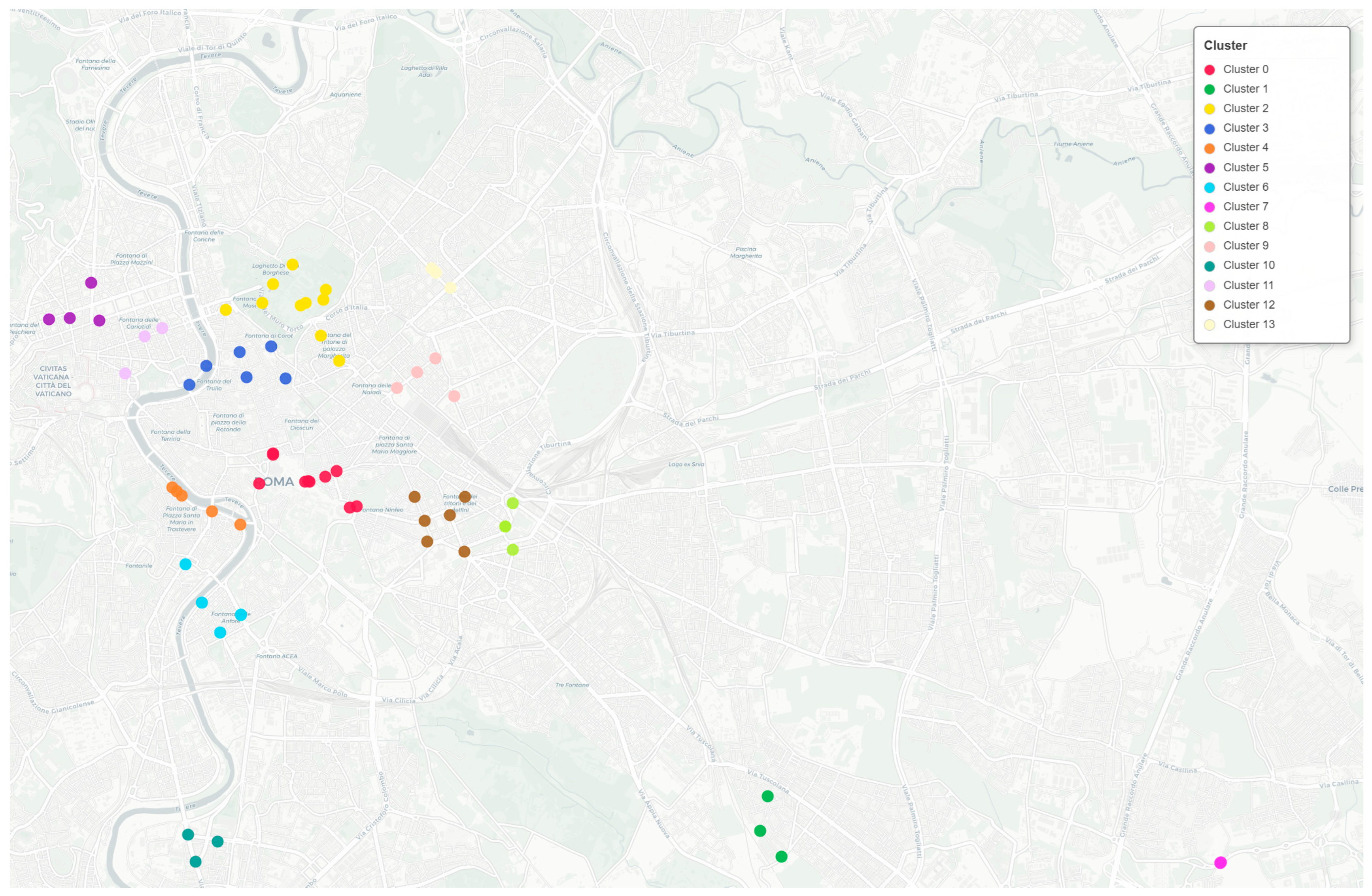
After identifying misclassified observations by the models, these are subjected to a spatial analysis using DBSCAN to determine whether the model’s errors are concentrated in specific areas of the city. For this model, an epsilon parameter of 50 m and MinPts equal to 3 have been used. The aim is to highlight the potential presence of latent variables that prevented the correct classification of bicycle crashes. It is important to note that this paragraph reports only the results from the OLR model; although it exhibits slightly lower predictive capabilities compared to the RF model, its high interpretability allows for a sharper focus on the problem.

As can be observed in Figure 6, most of the clusters representing model errors are concentrated in the city’s urban area, while only clusters 7, 8, and 10 represent more peripheral zones. Once the clusters have been identified, the relative frequencies of each variable within the cluster and the original dataset are calculated. Subsequently, Fisher’s exact test is performed—given the limited data within each cluster—instead of the chi-square test, to validate the latent factors. This approach is chosen for its robustness in handling the small sample sizes typical of the dense spatial clusters detected by DBSCAN.

Table 4. Cluster details in terms of variables and their values, frequency in the cluster and dataset, and variations, with the level of significance and p-value.

Cluster ID	Variable	Value	Cluster [%]	Dataset [%]	p-Value (Fisher)	Adj. p-Value
0	Road_Type	Two_way_carriageway	80.0%	45.8%	0.04643	0.04962
0	Food_service_establishments	Yes	90.0%	57.6%	0.04876	0.04962
0	Cyclist_Facilities	Yes	70.0%	30.5%	0.02201	0.04962
1	Collision_Partner	Car_Adults_25_65_Male	33.3%	0.0%	0.04348	0.04962
2	Pedestrian_Facilities	No	63.6%	5.2%	0.00003	0.00105
2	Hour	Afternoon_16_19	54.5%	22.4%	0.03876	0.04962
2	Transport_Facilities	No	100.0%	69.0%	0.02611	0.04962
2	Cyclist_Facilities	No	90.9%	58.6%	0.03822	0.04962
3	Road_Type	One_way_carriageway	83.3%	22.2%	0.00508	0.02466
3	Collision_Partner	No_Collision_Partner	100.0%	47.6%	0.01625	0.04962
3	Vehicular_flows	Vehicular_Flow < 500	83.3%	36.5%	0.03676	0.04962
4	Road_Type	One_way_carriageway	100.0%	21.9%	0.00103	0.00909
4	Collision_Partner	Powered_two_wheeler_Young_Under_25_Female	40.0%	0.0%	0.00426	0.02415
5	Road_Type	More_than_two_carriageways	50.0%	7.7%	0.04849	0.04962
5	Cyclist_Age	Elderly_over65	50.0%	7.7%	0.04849	0.04962
5	Collision_Partner	Powered_two_wheeler_Adults_25_65_Male	75.0%	21.5%	0.04366	0.04962
6	Collision_Partner	Powered_two_wheeler_Adults_25_65_Male	75.0%	21.5%	0.04366	0.04962
7	Cyclist_Age	Elderly_over65	100.0%	6.1%	0.00067	0.00909
7	Pedestrian_Facilities	No	100.0%	10.6%	0.00229	0.01557
7	Road_Type	Two_carriageways	66.7%	9.1%	0.03367	0.04962
7	Collision_Partner	Car_Adults_25_65_Female	33.3%	0.0%	0.04348	0.04962
7	Collision_Partner	Car_Young_Under_25_Male	33.3%	0.0%	0.04348	0.04962
7	Vehicular_speeds	Vehicular_Speed > 50	100.0%	33.3%	0.0439	0.04962
7	Food_service_establishments	No	100.0%	34.8%	0.04962	0.04962
8	Collision_Partner	Powered_two_wheeler_Adults_25_65_Male	75.0%	21.5%	0.04366	0.04962
8	Vehicular_speeds	Vehicular_Speed_30_50	75.0%	21.5%	0.04366	0.04962
9	Road_Type	More_than_two_carriageways	50.0%	7.7%	0.04849	0.04962
10	Road_Type	Two_carriageways	100.0%	7.6%	0.00107	0.00909
10	Collision_Partner	Heavy_vehicle_Young_Under_25_Male	33.3%	0.0%	0.04348	0.04962
10	Vehicular_speeds	Vehicular_Speed > 50	100.0%	33.3%	0.0439	0.04962
10	Educational_Facilities	Yes	66.7%	10.6%	0.04283	0.04962
12	Educational_Facilities	Yes	50.0%	9.5%	0.0259	0.04962
12	Transport_Facilities	Yes	66.7%	22.2%	0.03635	0.04962
13	Transport_Facilities	Yes	100.0%	22.7%	0.01557	0.04962

below reports the results of this analysis, specifically showing only the variables with a low p-value (i.e., the probability that the presence of that particular variable is due to chance). The Benjamini–Hochberg (BH) procedure to control for the False Discovery Rate (FDR) has also been used to control post hoc confirmation.

Starting with Cluster 0, the presence of cycle paths and food service establishments is 39% and 32% higher than in the original dataset, respectively, with a strong presence of two-way roads (see Table 4). According to OLR estimates, the presence of cycle paths and food service establishments typically acts as a mitigating factor. The high concentration of model errors recorded in this area may be due to the massive presence of cycling infrastructure, which, when combined with a high density of activities such as restaurants and cafes, can act as influential latent factors, thereby increasing the severity of the crashes. In this area of the city, given the potential for high interaction between different road users, more direct measures may be required in the future to ensure cyclists’ safety by reducing the number of interactions with other users.

Moving to Cluster 2, near the Villa Borghese Park, it is observed that most crashes occur between 4 and 7 p.m. Furthermore, there is a total absence of sidewalks in 63% of cases (compared to 5% in the original dataset), as well as no cycle paths or other transport facilities. In this specific cluster, the model may fail because the total absence of dedicated infrastructure during peak hours can create intense interactions between different modes of transport, exposing cyclists to a higher risk.

Spatially close to Cluster 2 is Cluster 3, located in an area between “Piazza del Popolo” and “Via Condotti”. This is a central, historic zone characterized by many narrow alleys (one-way streets) and low traffic flows. As shown in Table 4, 100% of the misclassified crashes occur when the cyclist hits an obstacle, falls alone, or hits a pedestrian. The model tends to predict an “uninjured” status rather than “injured” for low traffic flows, assuming a lower risk condition, which leads to incorrect classification. This can be explained by the presence of variables such as the road surface type (which differs from asphalt), high levels of road decay, or the heavy presence of tourist pedestrian flows, which are not introduced as variables in the model.

From Clusters 5, 6, and 8, located in fairly central areas, it emerges that the interaction between powered two-wheelers and cyclists identifies these as critical zones. Additionally, vehicle speeds between 30 and 50 km/h are recorded. This may signify busy urban areas characterized by a high modal share of two-wheeled vehicles or aggressive driving behavior that cannot be inferred from the data.

Cluster 7, identified in a more peripheral area, shows that most victims are cyclists over 65. Here, vehicle speeds are high (over 50 km/h), roads are dual carriageways, and there is a lack of infrastructure. The model highlights that the presence of elderly users—who are more susceptible to the risk of fatal accidents—coincides with high speeds. In this area, speed mitigation tools or the construction of dedicated cycling infrastructure may be necessary.

While the presence of schools or universities should theoretically mitigate crash severity according to the OLR model, Cluster 10 shows that 67% of crashes occur near educational facilities (compared to an 11% average). These occur on dual carriageways with speeds exceeding 50 km/h and a significant presence of heavy vehicles, such as public transport or commercial vehicles. An area showing such strong anomalies requires specifically calibrated interventions. In Clusters 12 and 13, consistent with Cluster 10, the high presence of transport facilities (100%) challenges the model, highlighting areas characterized by strong interaction between different modes of transport due to transit interchanges.

5. Discussion

Given the high class imbalance within the dataset (with fatal crashes representing only the 1.7%), the predictive capabilities of the model itself are inherently compromised by the scarcity of data belonging to the minority classes. While oversampling and weighting strategies in this case have been useful to improve the prediction of fatal crashes, on the other hand, this introduced noise and lower predictive performance capabilities toward the uninjured class. For these reasons, this methodology should be framed in the context of risk identification and spatial anomalies detection, rather than within the context of raw prediction tasks. The predictive performance of the OLR framework presented in this study aligns well with outcomes from more sophisticated severity models found in the literature. For instance, Das et al. [57] reported a McFadden’s pseudo-R² of 0.084 for a standard Logit Model (a value lower than the one obtained here), while their Mixed Logit specification achieved 0.4161. Similarly, other studies employing Mixed Logit formulations show varying results: Ye et al. [58] reached a McFadden value of 0.5090 in vehicle–e-bike crash analysis, whereas Chen et al. [59] and Wang et al. [60] reported values of 0.06 and 0.315, respectively. Furthermore, recent research by Scarano et al. [17] yielded a McFadden’s R² of 0.21 and an F1-score of 0.72 using a Mixed Logit approach, alongside a Random Forest model that achieved an F1-score of 0.88.

To contextualize the findings and critical variables obtained from the OLR and RF models, it is essential to benchmark them against the state of the art. In the literature review, according to Salmon et al. [61], no studies identify contributory factors outside the field of cyclists and road users; instead, few of them examine the relationships between contributory factors. The most common contributory factors analyzed are related to roadway, environment, cyclists, drivers, vehicles, and crash characteristics [17].

Among roadway factors, higher speed limits are associated with increased crash severity for cyclists involved in accidents [62], especially in rural areas where these high-speed limits are typically set [63]. Nighttime crashes are more likely to be severe [64], and the severity of accidents increases when they occur on motor vehicle lanes, on sidewalks, and at curves [62,65,66]. For these reasons, some authors suggest that separated cycle lanes increase safety levels by decreasing exposure to vehicle traffic [67].

Environmental contributory factors, such as rainy and foggy weather and unstable, slippery, and wet roads, increase the likelihood of serious crashes [68].

Older and younger cyclists are more likely to suffer a serious accident than other cyclists, such as male riders [63,69,70].

Other contributory factors in the field of cyclist behavior influence accident severity. Those include speeding, riding on the wrong side, mobile phone use, violations at intersections, not wearing helmets, and the state of alcohol impairment [71,72,73,74].

Driver-related factors, such as unwise overtaking and speeding, and the alcohol-impaired state [75], increase crash severity outcomes [76]. In addition, large and heavy vehicles [77] and crash types, such as head-on and angle crashes [78], lead to alarming crashes from the point of view of the outcome.

The results obtained within this study are largely in agreement with the literature examined on the topic and add an in-depth vision for a specific context, such as the city of Rome. As already noted in [62,63], vehicular speeds greater than 50 km/h, as it emerges from OLR, double the odds of a fatal outcome compared to lower and safer speeds (0–30 km/h). In line with the findings in [64], nighttime crashes between 8 p.m. and 6 a.m. are more dangerous than cyclist crashes during daytime, likely due to a lower level of overall visibility and higher speeds due to lower traffic volumes. Regarding demographic factors, this study supports what has already been seen in prior studies [63,69]: elderly cyclists, more than 65 years old, are the most vulnerable category of users. A critical risk factor, as emerges from this analysis, is the characteristic of the Collision_Partner vehicle profile. The results show that heavy vehicles are the most critical risk factor, with the highest OR [77]. According to the findings in [67], this study confirms the general trend of the role of cycling and pedestrian facilities as mitigation factors, but with some exceptions, as highlighted from the spatial error analysis.

An innovative contribution of this work regards the analysis of misclassified observations using DBSCAN, which highlights specific areas in the city where model predictions fail due to the presence of latent variables. While literature suggests that the presence of educational and commercial activities is beneficial to lowering the risk (likely due to the Safety in Numbers [79]), Cluster 0 and Cluster 10 obtained with the spatial analysis show an opposite trend. For instance, in Cluster 0, despite a high density of cycle lanes, the high presence of food service establishments hides the protective behavior associated with cyclist facilities. The latent variable behind this scenario is the high interactions between different users, suggesting that infrastructure presence is not protective if conflicts are not well managed. Similarly, the high presence of schools and universities in Cluster 10, with dual-carriageway roads and vehicular speeds higher than 50 km/h, overpowers the mitigating effects of educational facilities. From the analysis of Cluster 3, in the historical city center, with several one-way roads, with low vehicular traffic flows, it also emerges that this hotspot of anomalies could have been influenced by both low road surface quality and high interactions with pedestrian flows. In contrast, Cluster 10, identified in a peripheral area, shows that the combination of elderly cyclists and high-speed roads requires more targeted infrastructure interventions than the central area.

6. Conclusions

To study in detail the role of individual variables on cyclist crash severity and identify the main risk and mitigation factors in an urban context, an innovative methodological approach was introduced in this study. To obtain a detailed view of individual crashes, crash data were enriched with three different datasets (vehicular flows, vehicular speeds, and geographic characteristics), thus performing a data fusion of different sources. Subsequently, a Random Forest (RF) and an Ordered Logit Regression (OLR) were developed not only for prediction purposes but also for a detailed analysis of contributing factors. Using the misclassified observations, clusters were created via DBSCAN to identify potential risk zones exhibiting anomalous behavior due to latent factors. By combining statistical analyses such as Fisher’s exact test, latent variables within these clusters are identified.

What emerges from the results of these analyses is that the presence of cycle paths plays a risk-mitigating role. Additionally, in suburban contexts, the probability of a fatal crash is lower than in an urban one. The analyses also reveal that the presence of anthropic activities, such as shops, schools, and universities, acts as a mitigation factor for cyclist risk. Conversely, vehicular speed and the strong presence of heavy vehicles emerge as the main detected risk factors.

The analysis of anomalous clusters and latent variables reveals that, where strong interactions occur between different traffic flows and modes due to the presence of food service establishments, the protective role of cycle paths could be reduced. It was also found that in central and historic zones, given the presence of several one-way streets and low traffic flows, strong interaction with pedestrian flows can create risk scenarios, potentially exacerbated by the presence of uneven road surfaces.

Among the innovative aspects introduced in this work, it is worth mentioning the data fusion of different sources to enhance the informational value of the enriched dataset, particularly to understand the role of vehicular speed and flows on cyclist crashes. Another key aspect is the combined use of Machine Learning and Econometric Models, such as OLR, alongside models like DBSCAN to perform spatial analysis and identify anomalous risk areas requiring particular attention. This approach not only improved understanding of various mitigation and risk factors but also allowed for the application of severity models to real-world contexts and spatial analyses.

Despite the innovative aspects introduced, the study is characterized by some limitations. First, only one city is analyzed, whereas a comparison between different contexts could have highlighted further aspects. Additionally, the lack of integration of these cyclist crash data with pedestrian and cycling flows must be noted. These limitations naturally represent a starting point for future analyses. Therefore, future developments of this work could involve the integration and enrichment of the dataset with new variables, such as socio-economic and pavement-related ones. Recent work has shown that both infrastructure lighting quality and cyclist visibility significantly influence crash severity outcomes. For instance, Fryc et al. [80] demonstrates how lighting infrastructure and cyclist-mounted lighting systems affect nighttime safety. Given that several identified clusters show elevated nighttime crashes, incorporating both street lighting data and information about cyclist lighting equipment could explain some of the unexplained spatial variation.

Furthermore, to extend the sample size of crashes examined, collecting more recent data will be necessary. It also emerges that the translation of detected patterns into specific engineering countermeasures is constrained by the temporal resolution of the available data. Since the analysis relies on quarterly aggregated crash records, it captures structural and recurrent risk patterns rather than transient or event-specific causes (e.g., temporary work zones or anomalous congestion events). Therefore, the identified clusters should not be interpreted as immediate prescriptions for geometric redesign, but rather as priority zones for in situ safety audits. Finally, from a modeling perspective, new machine learning or Econometric Models, such as Generalized Ordered Logit or Random Parameter Logit, could be implemented to improve the predictive capabilities of the OLR.

References

1. World Report on Road Traffic Injury Prevention. Available online: https://www.who.int/publications/i/item/9241562609 (accessed on 2 December 2025).
2. First Global Ministerial Conference on Road Safety. Available online: https://www.who.int/publications/m/item/first-global-ministerial-conference-on-road-safety (accessed on 2 December 2025).
3. Decade of Action for Road Safety 2011–2020. Available online: https://www.who.int/groups/united-nations-road-safety-collaboration/decade-of-action-for-road-safety-2011-2020 (accessed on 2 December 2025).
4. Decade of Action for Road Safety 2021–2030. Available online: https://www.who.int/teams/social-determinants-of-health/safety-and-mobility/decade-of-action-for-road-safety-2021-2030 (accessed on 2 December 2025).
5. Nations, U. United Nations Conference on the Human Environment, Stockholm 1972. Available online: https://www.un.org/en/conferences/environment/stockholm1972 (accessed on 2 December 2025).
6. Directorate-General for Mobility and Transport (European Commission). Next Steps Towards ‘Vision Zero’: EU Road Safety Policy Framework 2021 2030; Publications Office of the European Union: Luxembourg, 2020; ISBN 978-92-76-13219-6. [Google Scholar]
7. Global Status Report on Road Safety 2023. Available online: https://www.who.int/teams/social-determinants-of-health/safety-and-mobility/global-status-report-on-road-safety-2023 (accessed on 2 December 2025).
8. Schepers, P.; Helbich, M.; Hagenzieker, M.; de Geus, B.; Dozza, M.; Agerholm, N.; Niska, A.; Airaksinen, N.; Papon, F.; Gerike, R. The Development of Cycling in European Countries since 1990. Eur. J. Transp. Infrastruct. Res. 2021, 21, 41–70. [Google Scholar] [CrossRef]
9. Schepers, P.; Stipdonk, H.; Methorst, R.; Olivier, J. Bicycle Fatalities: Trends in Crashes with and without Motor Vehicles in The Netherlands. Transp. Res. Part F Traffic Psychol. Behav. 2017, 46, 491–499. [Google Scholar] [CrossRef]
10. Uijtdewilligen, T.; Ulak, M.B.; Wijlhuizen, G.J.; Bijleveld, F.; Dijkstra, A.; Geurs, K.T. How Does Hourly Variation in Exposure to Cyclists and Motorised Vehicles Affect Cyclist Safety? A Case Study from a Dutch Cycling Capital. Saf. Sci. 2022, 152, 105740. [Google Scholar] [CrossRef]
11. Wegman, F.; Schepers, P. Safe System Approach for Cyclists in the Netherlands: Towards Zero Fatalities and Serious Injuries? Accid. Anal. Prev. 2024, 195, 107396. [Google Scholar] [CrossRef]
12. Kale, N.N.; Lavorgna, T.; Vemulapalli, K.C.; Ierulli, V.; Mulcahey, M.K. Traumatic Orthopaedic Motor Vehicle Injuries: Are There Age and Sex Differences in Pedestrian and Cyclist Accidents in a Major Urban Center? Injury 2023, 54, 1484–1491. [Google Scholar] [CrossRef]
13. Meuleners, L.B.; Fraser, M.; Johnson, M.; Stevenson, M.; Rose, G.; Oxley, J. Characteristics of the Road Infrastructure and Injurious Cyclist Crashes Resulting in a Hospitalisation. Accid. Anal. Prev. 2020, 136, 105407. [Google Scholar] [CrossRef]
14. Schepers, J.; Kroeze, P.; Sweers, W.; Wüst, J. Road Factors and Bicycle–Motor Vehicle Crashes at Unsignalized Priority Intersections. Accid. Anal. Prev. 2011, 43, 853–861. [Google Scholar] [CrossRef]
15. Zhou, N.; Zeng, H.; Xie, R.; Yang, T.; Kong, J.; Song, Z.; Zhang, F.; Liao, X.; Chen, X.; Miao, Q. Analysis of Road Traffic Accidents and Casualties Associated with Electric Bikes and Bicycles in Guangzhou, China: A Retrospective Descriptive Analysis. Heliyon 2024, 10, e29961. [Google Scholar] [CrossRef]
16. Ekmekci, M.; Dadashzadeh, N.; Woods, L. Assessing the Impact of Low-Speed Limit Zones’ Policy Implications on Cyclist Safety: Evidence from the UK. Transp. Policy 2024, 152, 29–39. [Google Scholar] [CrossRef]
17. Scarano, A.; Riccardi, M.R.; Mauriello, F.; D’Agostino, C.; Pasquino, N.; Montella, A. Injury Severity Prediction of Cyclist Crashes Using Random Forests and Random Parameters Logit Models. Accid. Anal. Prev. 2023, 192, 107275. [Google Scholar] [CrossRef]
18. Engbers, C.; Dubbeldam, R.; Brusse-Keizer, M.; Buurke, J.; De Waard, D.; Rietman, J. Characteristics of Older Cyclists (65+) and Factors Associated with Self-Reported Cycling Accidents in the Netherlands. Transp. Res. Part F Traffic Psychol. Behav. 2018, 56, 522–530. [Google Scholar] [CrossRef]
19. De Geus, B.; Vandenbulcke, G.; Panis, L.I.; Thomas, I.; Degraeuwe, B.; Cumps, E.; Aertsens, J.; Torfs, R.; Meeusen, R. A Prospective Cohort Study on Minor Accidents Involving Commuter Cyclists in Belgium. Accid. Anal. Prev. 2012, 45, 683–693. [Google Scholar] [CrossRef] [PubMed]
20. Värnild, A.; Tillgren, P.; Larm, P. Road Users Seriously Injured in Single Crashes–The Impact of Sex, Age and Speed Limit on Injuries for Pedestrians, Cyclists, Car Occupants and Motorcyclists in Sweden, 2016–2019. J. Transp. Health 2023, 33, 101717. [Google Scholar] [CrossRef]
21. Eriksson, J.; Niska, A.; Forsman, Å. Injured Cyclists with Focus on Single-Bicycle Crashes and Differences in Injury Severity in Sweden. Accid. Anal. Prev. 2022, 165, 106510. [Google Scholar] [CrossRef] [PubMed]
22. Meredith, L.; Kovaceva, J.; Bálint, A. Mapping Fractures from Traffic Accidents in Sweden: How Do Cyclists Compare to Other Road Users? Traffic Inj. Prev. 2020, 21, 209–214. [Google Scholar] [CrossRef]
23. Guirao, B.; Gálvez-Pérez, D.; Casado-Sanz, N. The Impact of the Cyclist Infrastructure Type on Bike Accidents: The Experience of Madrid. Transp. Res. Procedia 2023, 71, 403–410. [Google Scholar] [CrossRef]
24. Billot-Grasset, A.; Amoros, E.; Hours, M. How Cyclist Behavior Affects Bicycle Accident Configurations? Transp. Res. Part F Traffic Psychol. Behav. 2016, 41, 261–276. [Google Scholar]
25. Italian Institute of Statistics. Istat. Available online: https://www.istat.it/tag/incidenti/ (accessed on 20 January 2026).
26. Svetnik, V.; Liaw, A.; Tong, C.; Culberson, J.C.; Sheridan, R.P.; Feuston, B.P. Random Forest: A Classification and Regression Tool for Compound Classification and QSAR Modeling. J. Chem. Inf. Comput. Sci. 2003, 43, 1947–1958. [Google Scholar] [CrossRef]
27. Meyer, D.; Leisch, F.; Hornik, K. The Support Vector Machine under Test. Neurocomputing 2003, 55, 169–186. [Google Scholar] [CrossRef]
28. Bylander, T. Estimating Generalization Error on Two-Class Datasets Using out-of-Bag Estimates. Mach. Learn. 2002, 48, 287–297. [Google Scholar] [CrossRef]
29. Breiman, L. Random Forests. Mach. Learn. 2001, 45, 5–32. [Google Scholar] [CrossRef]
30. Liaw, A.; Wiener, M. Classification and Regression by randomForest. R News 2002, 2, 18–22. [Google Scholar]
31. James, G.; Witten, D.; Hastie, T.; Tibshirani, R. An Introduction to Statistical Learning: With Applications in R; Springer: New York, NY, USA, 2013; Volume 103. [Google Scholar]
32. Yan, M.; Shen, Y. Traffic Accident Severity Prediction Based on Random Forest. Sustainability 2022, 14, 1729. [Google Scholar] [CrossRef]
33. Ho, T.K. Random Decision Forests; IEEE: Montreal, QC, Canada, 1995; Volume 1, pp. 278–282. [Google Scholar]
34. Chen, M.-M.; Chen, M.-C. Modeling Road Accident Severity with Comparisons of Logistic Regression, Decision Tree and Random Forest. Information 2020, 11, 270. [Google Scholar] [CrossRef]
35. Elyassami, S.; Hamid, Y.; Habuza, T. Road Crashes Analysis and Prediction Using Gradient Boosted and Random Forest Trees; IEEE: Montreal, QC, Canada, 2021; pp. 520–525. [Google Scholar]
36. Gatera, A.; Kuradusenge, M.; Bajpai, G.; Mikeka, C.; Shrivastava, S. Comparison of Random Forest and Support Vector Machine Regression Models for Forecasting Road Accidents. Sci. Afr. 2023, 21, e01739. [Google Scholar] [CrossRef]
37. Archer, K.J.; Kimes, R.V. Empirical Characterization of Random Forest Variable Importance Measures. Comput. Stat. Data Anal. 2008, 52, 2249–2260. [Google Scholar] [CrossRef]
38. Rella Riccardi, M.; Mauriello, F.; Sarkar, S.; Galante, F.; Scarano, A.; Montella, A. Parametric and Non-Parametric Analyses for Pedestrian Crash Severity Prediction in Great Britain. Sustainability 2022, 14, 3188. [Google Scholar] [CrossRef]
39. Cappelli, G.; Nardoianni, S.; D’Apuzzo, M.; Nicolosi, V. Interpretable Crash Severity Prediction Models to Improve Cyclist Safety; Springer: Cham, Switzerland, 2025; pp. 319–334. [Google Scholar]
40. Hosmer, D.W., Jr.; Lemeshow, S.; Sturdivant, R.X. Applied Logistic Regression; John Wiley & Sons: Hoboken, NJ, USA, 2013; ISBN 1-118-54835-3. [Google Scholar]
41. Macioszek, E.; Granà, A. The Analysis of the Factors Influencing the Severity of Bicyclist Injury in Bicyclist-Vehicle Crashes. Sustainability 2021, 14, 215. [Google Scholar] [CrossRef]
42. Nick, T.G.; Campbell, K.M. Logistic Regression. In Topics in Biostatistics; Humana Press: Totowa, NJ, USA, 2007; pp. 273–301. [Google Scholar]
43. Mannering, F.; Bhat, C.R.; Shankar, V.; Abdel-Aty, M. Big Data, Traditional Data and the Tradeoffs between Prediction and Causality in Highway-Safety Analysis. Anal. Methods Accid. Res. 2020, 25, 100113. [Google Scholar] [CrossRef]
44. Liu, J.; Khattak, A.J.; Li, X.; Nie, Q.; Ling, Z. Bicyclist Injury Severity in Traffic Crashes: A Spatial Approach for Geo-Referenced Crash Data to Uncover Non-Stationary Correlates. J. Saf. Res. 2020, 73, 25–35. [Google Scholar] [CrossRef]
45. Washington, S.; Karlaftis, M.G.; Mannering, F.; Anastasopoulos, P. Statistical and Econometric Methods for Transportation Data Analysis; Chapman and Hall: Boca Raton, FL, USA, 2020; ISBN 0-429-24401-0. [Google Scholar]
46. Train, K.E. Discrete Choice Methods with Simulation; Cambridge University Press: Cambridge, UK, 2009; ISBN 1-139-48037-5. [Google Scholar]
47. Shen, J.; Wang, T.; Zheng, C.; Yu, M. Determinants of Bicyclist Injury Severity Resulting from Crashes at Roundabouts, Crossroads, and T-Junctions. J. Adv. Transp. 2020, 2020, 6513128. [Google Scholar] [CrossRef]
48. Stipancic, J.; Zangenehpour, S.; Miranda-Moreno, L.; Saunier, N.; Granié, M.-A. Investigating the Gender Differences on Bicycle-Vehicle Conflicts at Urban Intersections Using an Ordered Logit Methodology. Accid. Anal. Prev. 2016, 97, 19–27. [Google Scholar] [CrossRef] [PubMed]
49. Oh, S.-H. Error Back-Propagation Algorithm for Classification of Imbalanced Data. Neurocomputing 2011, 74, 1058–1061. [Google Scholar] [CrossRef]
50. Ester, M.; Kriegel, H.-P.; Sander, J.; Xu, X. A Density-Based Algorithm for Discovering Clusters in Large Spatial Databases with Noise; University of Munic: Munich, Germany, 1996; Volume 96, pp. 226–231. [Google Scholar]
51. MacQueen, J. Multivariate Observations. In Proceedings ofthe 5th Berkeley Symposium on Mathematical Statisticsand Probability; University of California Press: Oakland, CA, USA, 1967; Volume 1, pp. 281–297. [Google Scholar]
52. Ram, A.; Jalal, S.; Jalal, A.S.; Kumar, M. A Density Based Algorithm for Discovering Density Varied Clusters in Large Spatial Databases. Int. J. Comput. Appl. 2010, 3, 1–4. [Google Scholar] [CrossRef]
53. Topcuoglu, B.; Memisoglu Baykal, T.; Tuydes Yaman, H. Speed-Related Traffic Accident Analysis Using GIS-Based DBSCAN and NNH Clustering. Int. Arch. Photogramm. Remote Sens. Spat. Inf. Sci. 2022, 48, 487–494. [Google Scholar] [CrossRef]
54. Khan, K.; Rehman, S.U.; Aziz, K.; Fong, S.; Sarasvady, S. DBSCAN: Past, present and future. In The fifth International Conference on the Applications of Digital Information and Web Technologies; Amrita University: Chennai, India, 2014; Volume 96, pp. 232–238. [Google Scholar]
55. Zhang, M.; Fu, R.; Guo, Y.; Wang, L.; Wang, P.; Deng, H. Cyclist Detection and Tracking Based on Multi-Layer Laser Scanner. Hum.-Centric Comput. Inf. Sci. 2020, 10, 20. [Google Scholar] [CrossRef]
56. Chawla, N.V.; Bowyer, K.W.; Hall, L.O.; Kegelmeyer, W.P. SMOTE: Synthetic Minority over-Sampling Technique. J. Artif. Intell. Res. 2002, 16, 321–357. [Google Scholar] [CrossRef]
57. Das, S.; Tamakloe, R.; Zubaidi, H.; Obaid, I.; Rahman, M.A. Bicyclist Injury Severity Classification Using a Random Parameter Logit Model. Int. J. Transp. Sci. Technol. 2023, 12, 1093–1108. [Google Scholar] [CrossRef]
58. Ye, F.; Wang, C.; Cheng, W.; Liu, H. Exploring Factors Associated with Cyclist Injury Severity in Vehicle-Electric Bicycle Crashes Based on a Random Parameter Logit Model. J. Adv. Transp. 2021, 2021, 5563704. [Google Scholar] [CrossRef]
59. Chen, C.; Anderson, J.C.; Wang, H.; Wang, Y.; Vogt, R.; Hernandez, S. How Bicycle Level of Traffic Stress Correlate with Reported Cyclist Accidents Injury Severities: A Geospatial and Mixed Logit Analysis. Accid. Anal. Prev. 2017, 108, 234–244. [Google Scholar] [CrossRef]
60. Wang, T.; Chen, J.; Wang, C.; Ye, X. Understand E-Bicyclist Safety in China: Crash Severity Modeling Using a Generalized Ordered Logit Model. Adv. Mech. Eng. 2018, 10, 1687814018781625. [Google Scholar] [CrossRef]
61. Salmon, P.M.; Naughton, M.; Hulme, A.; McLean, S. Bicycle Crash Contributory Factors: A Systematic Review. Saf. Sci. 2022, 145, 105511. [Google Scholar] [CrossRef]
62. Wang, Z.; Neitzel, R.L.; Zheng, W.; Wang, D.; Xue, X.; Jiang, G. Road Safety Situation of Electric Bike Riders: A Cross-Sectional Study in Courier and Take-out Food Delivery Population. Traffic Inj. Prev. 2021, 22, 564–569. [Google Scholar] [CrossRef] [PubMed]
63. Hosseinpour, M.; Madsen, T.K.O.; Olesen, A.V.; Lahrmann, H. An In-Depth Analysis of Self-Reported Cycling Injuries in Single and Multiparty Bicycle Crashes in Denmark. J. Saf. Res. 2021, 77, 114–124. [Google Scholar] [CrossRef] [PubMed]
64. Dash, I.; Abkowitz, M.; Philip, C. Factors Impacting Bike Crash Severity in Urban Areas. J. Saf. Res. 2022, 83, 128–138. [Google Scholar] [CrossRef]
65. Gitelman, V.; Korchatov, A.; Carmel, R. Safety-Related Behaviours of e-Cyclists on Urban Streets: An Observational Study in Israel. Transp. Res. Procedia 2022, 60, 609–616. [Google Scholar] [CrossRef]
66. Alshehri, A.; Eustace, D.; Hovey, P. Analysis of Factors Affecting Crash Severity of Pedestrian and Bicycle Crashes Involving Vehicles at Intersections; American Society of Civil Engineers: Reston, VA, USA, 2020; pp. 49–58. [Google Scholar]
67. Loo, B.P.; Tsui, K. Bicycle Crash Casualties in a Highly Motorized City. Accid. Anal. Prev. 2010, 42, 1902–1907. [Google Scholar] [CrossRef]
68. Samerei, S.A.; Aghabayk, K.; Shiwakoti, N.; Mohammadi, A. Using Latent Class Clustering and Binary Logistic Regression to Model Australian Cyclist Injury Severity in Motor Vehicle–Bicycle Crashes. J. Saf. Res. 2021, 79, 246–256. [Google Scholar] [CrossRef]
69. Bahrololoom, S.; Young, W.; Logan, D. Modelling Injury Severity of Bicyclists in Bicycle-Car Crashes at Intersections. Accid. Anal. Prev. 2020, 144, 105597. [Google Scholar] [CrossRef]
70. Weber, T.; Scaramuzza, G.; Schmitt, K.-U. Evaluation of E-Bike Accidents in Switzerland. Accid. Anal. Prev. 2014, 73, 47–52. [Google Scholar] [CrossRef]
71. Behnood, A.; Roshandeh, A.M.; Mannering, F.L. Latent Class Analysis of the Effects of Age, Gender, and Alcohol Consumption on Driver-Injury Severities. Anal. Methods Accid. Res. 2014, 3, 56–91. [Google Scholar] [CrossRef]
72. Bueth, C.M.; Barbour, N.; Abdel-Aty, M. Effectiveness of Bicycle Helmets and Injury Prevention: A Systematic Review of Meta-Analyses. Sci. Rep. 2023, 13, 8540. [Google Scholar] [CrossRef] [PubMed]
73. Hamann, C.J.; Peek-Asa, C.; Lynch, C.F.; Ramirez, M.; Hanley, P. Epidemiology and Spatial Examination of Bicycle-Motor Vehicle Crashes in Iowa, 2001–2011. J. Transp. Health 2015, 2, 178–188. [Google Scholar] [CrossRef] [PubMed]
74. Behnood, A.; Mannering, F. Determinants of Bicyclist Injury Severities in Bicycle-Vehicle Crashes: A Random Parameters Approach with Heterogeneity in Means and Variances. Anal. Methods Accid. Res. 2017, 16, 35–47. [Google Scholar] [CrossRef]
75. Calvi, A.; D’Amico, F.; Ferrante, C.; Bianchini Ciampoli, L. Driving Simulator Study for Evaluating the Effectiveness of Virtual Warnings to Improve the Safety of Interaction between Cyclists and Vehicles. Transp. Res. Rec. 2022, 2676, 436–447. [Google Scholar] [CrossRef]
76. Liu, S.; Fan, W. Investigating Factors Affecting Injury Severity in Bicycle–Vehicle Crashes: A Day-of-Week Analysis with Partial Proportional Odds Logit Models. Can. J. Civ. Eng. 2021, 48, 941–947. [Google Scholar] [CrossRef]
77. Sun, Z.; Xing, Y.; Gu, X.; Chen, Y. Influence Factors on Injury Severity of Bicycle-Motor Vehicle Crashes: A Two-Stage Comparative Analysis of Urban and Suburban Areas in Beijing. Traffic Inj. Prev. 2022, 23, 118–124. [Google Scholar] [CrossRef]
78. Oikawa, S.; Matsui, Y.; Nakadate, H.; Aomura, S. Factors in Fatal Injuries to Cyclists Impacted by Five Types of Vehicles. Int. J. Automot. Technol. 2019, 20, 197–205. [Google Scholar] [CrossRef]
79. Tasic, I.; Elvik, R.; Brewer, S. Exploring the Safety in Numbers Effect for Vulnerable Road Users on a Macroscopic Scale. Accid. Anal. Prev. 2017, 109, 36–46. [Google Scholar] [CrossRef]
80. Fryc, I.; Listowski, M.; Fan, J.; Czyżewski, D. Energy-Efficient and Smart Bicycle Lamps: A Comprehensive Review. Energies 2024, 17, 5335. [Google Scholar] [CrossRef]
Figure 1. The adopted methodology is summarized in this flow chart. It is worth noting that three main phases could be identified as data fusion, crash injury severity model calibration, and spatial analysis.
Urbansci 10 00073 g001
Figure 2. A spatial distribution of cyclist crashes in the city of Rome. Red dots represent Fatal crashes, while yellow and green dots represent Injured and Uninjured crashes, respectively. The administrative border of the municipality is drawn in blue.
Urbansci 10 00073 g002
Figure 3. (a) CM of the RF model is shown (it is worth remembering that this CM is evaluated on the test set, which corresponds to 30% of the whole dataset); (b) CM of the weighted OLR model, evaluated on the whole dataset.
Urbansci 10 00073 g003
Figure 4. The most important factors related to cyclist crashes, according to the Importance Score obtained with RF.
Urbansci 10 00073 g004
Figure 5. Graphical output of the most important contributing factors: variables with an OR > 1 represent risk factors, while variables with OR < 1 represent mitigation factors (the red dot line represents OR = 1). Significance levels: *** p < 0.001, ** p < 0.01, * p < 0.05.
Urbansci 10 00073 g005
Figure 6. Graphical results of cluster analysis with the DBSCAN algorithm.
Urbansci 10 00073 g006