Article

Auditing iRAP’s ViDA Risk Engine: A Two-Stage Surrogate Learning and Orthogonalized Heterogeneity Framework for Modelled Road Safety

by
Amirhossein Hassani
*,
Borna Abramović
,
Muhammad Shahid
and
Marko Ševrović
Faculty of Transport and Traffic Sciences, University of Zagreb, 10000 Zagreb, Croatia
*
Author to whom correspondence should be addressed.
Infrastructures 2026, 11(4), 129; https://doi.org/10.3390/infrastructures11040129
Submission received: 2 March 2026 / Revised: 24 March 2026 / Accepted: 1 April 2026 / Published: 5 April 2026

Abstract

Road safety studies commonly use machine learning to predict crashes or to estimate crash-based treatment effects. This study instead audits the modelled fatal-and-serious-injury (FSI) risk produced by the iRAP ViDA risk engine. We analyse 147,466 segments (100 m each) from 12 surveys grouped into four European reporting groups. In Stage 1, gradient-boosted trees reproduce the engine’s risk surface under road-grouped cross-validation(R2 ≈ 0.92 with flows and survey identifiers), and Shapley-based attributions identify which coded attributes drive modelled risk at 396 hotspots (top-three segments per road). In Stage 2, a causal-forest double machine learning estimator adjusts for 38 covariates to estimate segment-level conditional contrasts between modelled risk and six retrofittable treatments across all eligible segments. Simple absolute and relative reduction thresholds translate these associations into 1170 association-based candidate upgrades. On 321 over-lapping hotspots, the candidate upgrades show moderate agreement with iRAP’s Safer Roads Investment Plan (Recall = 0.77; Precision = 0.66; Cohen’s κ = 0.40). All results are conditional associations on a calibrated risk engine whose totals are anchored to project- or network-level fatality totals or fatality estimates used in calibration, not causal effects on observed crashes.

1. Introduction

This section situates the study within the road safety and infrastructure risk modelling landscape, identifies gaps in current practice, and states the research questions and contributions.

1.1. Background and Motivation

Road traffic injuries remain a persistent global crisis, claiming an estimated 1.19 million lives annually and representing a leading cause of death for children and young adults [1]. The economic burden is similarly severe, costing countries, particularly low- and middle-income countries (LMICs), around 3% of GDP, with some settings such as Tanzania reporting losses as high as 10.5% of GDP [2]. Road trauma is therefore a major public health and development challenge, with disproportionately high burdens on LMICs. Synthesis work on road safety in these contexts highlights persistent gaps in infrastructure safety, crash data quality, and local evaluation capacity, even after the first Decade of Action for Road Safety [3,4]. At the same time, substantial investment is being directed toward upgrading roads, often guided by infrastructure-focused safety assessment tools and generic crash modification factors (CMFs).
A growing body of empirical work has demonstrated that the safety effect of a given countermeasure depends strongly on the context. Classical CMF studies for roadside barriers, shoulders, and cross-sectional elements show that the estimated effects vary across traffic volume, curvature, and speed environments [5,6,7,8]. More recent work using flexible models and causal inference finds strong heterogeneity by crash type, geometry, and user group. Examples include motorcycle-involved crashes and mountainous freeway settings [9,10,11]. Simulation-based evaluations confirm that segment-level treatment effects can differ substantially from global CMFs when multiple countermeasures are combined [12]. Observed effects range from clear reductions in severe crashes to small or even adverse changes, suggesting that a single global CMF can hide important site-level differences and may be a poor guide to where an intervention is most effective.
At the same time, many countries and development banks are adopting advanced road assessment tools that focus on infrastructure risk rather than waiting for crashes to accumulate. The International Road Assessment Programme (iRAP) and its ViDA platform [13] are now widely used to produce star ratings and investment plans from standardised infrastructure surveys [14,15]. These tools have helped harmonise coding practice and create a common language around infrastructure risk, but they remain largely rule-based and do not yet exploit the full range of statistical and machine learning tools now available.
In parallel, machine learning has become common in crash prediction and injury-severity modelling. Reviews report extensive use of gradient boosting, random forests, deep learning, and heterogeneous ensembles for crash frequency and injury-severity prediction [16,17,18,19]. These models can improve predictive accuracy by capturing nonlinearities and high-order interactions, yet there is growing concern about their use for planning interventions. Predictive feature importance and post hoc explainers such as Shapley Additive exPlanations (SHAP) are sensitive to model specification, do not identify causal effects on their own, and can be difficult to interpret for policy [20,21].
Recent work has therefore started to bring causal machine learning into road safety. Generalized random forests and causal forests are being used to estimate heterogeneous treatment effects for infrastructure changes and operational interventions, and double-robust and double machine learning (DML) methods have been applied to study how crashes affect traffic and to investigate determinants of incident duration [11,22,23,24,25]. These methods target treatment-effect estimation under assumptions such as conditional exchangeability and overlap and are designed to explore which sites benefit most from an intervention rather than only predicting risk.
Together, this literature suggests two needs. First, proactive infrastructure risk models such as iRAP should be examined statistically rather than treated as operational systems whose outputs are often accepted without statistical audit. Second, any attempt to move from prediction to recommendation should be grounded in causal reasoning, with clear assumptions and careful use of machine learning rather than relying only on predictive accuracy or feature importance.
In practical terms, ViDA combines coded infrastructure attributes, traffic and vulnerable road user flows, and project calibration inputs to produce segment-level modelled fatal-and-serious-injury (FSI) estimates and a Safer Roads Investment Plan (SRIP) of candidate countermeasures [14,15,26]. FSI is the modelled annual expected number of fatalities plus serious injuries for a 100 m segment, while SRIP is the rule-based recommendation module. This study examines those exported ViDA outputs. It does not build a crash prediction model from scratch using observed crash counts.
Traditional regression, mixed-effects, and random-parameter models remain central in road-safety research, especially when the outcome is observed crash frequency or injury severity [27,28,29]. The present task is different. In Stage 1, we ask whether a flexible model can reproduce ViDA’s own segment-level modelled FSI from the exported inputs and recover the same hotspot ranking under road-grouped validation. In Stage 2, we ask whether the association between candidate upgrades and the exported modelled FSI varies across observed coded road contexts, rather than imposing a single average coefficient for all segments or estimating latent random parameters from observed crash counts. This is why we use flexible tree-based learning in Stage 1 and causal forests in Stage 2, while interpreting the latter as conditional associations on the ViDA surface rather than direct crash effects.
The present study therefore takes the ViDA-modelled fatal-and-serious-injury (FSI) estimate as its outcome. In the iRAP model, coded infrastructure attributes, traffic and vulnerable road user flows, and project calibration inputs are combined to produce a modelled number of fatalities and serious injuries per 100 m segment [15,26]. This modelled FSI is available for every surveyed segment immediately after coding, provides a continuous risk metric, and avoids reliance on sparse segment-level crash records [30,31]. In the pooled corpus used here, it is the common segment-level outcome available across surveys. At the same time, it is a model output, not an observed outcome. Crucially, however, ViDA’s calibration stage anchors modelled fatality totals to project- or network-level fatality totals or fatality estimates used in calibration [15,26], and these totals are then distributed deterministically across segments by fixed rules. This hybrid character, calibration-anchored at the network level and deterministically allocated at the segment level, makes the modelled FSI a useful audit target. A data-driven surrogate can show whether the allocation rules distribute risk in ways that are consistent with known infrastructure–crash relationships. Any findings must still be framed as associations on the modelled risk surface rather than as direct estimates of crash effects.

1.2. Gaps in Current Practice

Despite progress in both infrastructure risk modelling and data-driven methods, current practice leaves several gaps. First, most iRAP-based applications treat the ViDA engine as a closed system and do not statistically analyse its outputs. They use star ratings and investment plans directly, without investigating which attributes the model is most sensitive to in a given region or how that sensitivity varies across networks. Second, many crash prediction studies use machine learning to forecast risk, but stop at hotspot identification and do not quantify how standard countermeasures might change risk at specific sites [16,17,32]. Third, even when infrastructure effects are studied, they are often summarised as global crash modification factors that ignore the heterogeneity documented in recent work (e.g., [5,7,23]; see Section 2).
Finally, the emerging causal machine learning literature on transport has so far focused mostly on observed crashes, incident duration, and traffic impacts [11,22,24,25]. There is little work on how these methods could be used on top of an established infrastructure risk model, such as iRAP, to generate segment-level treatment associations on a modelled risk surface and to compare those associations with the recommendations produced by the rule-based system. This is an important gap, because iRAP and similar tools are already embedded in the funding and design workflows. Understanding where the Stage 2 association model agrees or disagrees with ViDA and why is directly relevant for agencies that need to prioritise limited budgets. In the following sections, we use the modelled FSI as the outcome of a two-stage learning framework.

1.3. Aim, Research Questions, and Contributions

This paper studies how to audit a calibrated, deterministic infrastructure risk engine when only exported segment-level outputs are available. We treat ViDA’s modelled FSI as a fixed response surface over coded attributes and flows. The present paper therefore does not ask whether ViDA predicts observed crashes better than a separate crash model. Instead, we ask whether modern learning methods can (i) reproduce that surface under road-grouped generalisation, (ii) identify high-risk segments consistently with the engine, and (iii) estimate which actionable attribute upgrades are associated with lower modelled risk after adjusting for coded context. Because Stage 1 learns from exported inputs that are closely related to the ViDA engine inputs, it should be interpreted as an internal audit of how well the exported inputs reproduce the ViDA pattern, rather than as external validation against observed crash outcomes. A crash-based external validation study would be valuable, but it would require harmonized segment-level observed crash histories and aligned exposure and time windows across surveys, which is a different design from the present audit.
We address four research questions:
  • Emulation fidelity. How accurately can a surrogate model approximate the ViDA modelled-FSI surface under grouped-by-road cross-validation, and how sensitive is this fidelity to exposure/speed inputs and survey identifiers?
  • Hotspot retrieval. If hotspots are defined as the Top-K segments per road, how well do out-of-fold surrogate predictions recover the engine-defined Top-K set, and how sensitive are results to K?
  • Conditional contrasts for actionable upgrades. For a restricted set of retrofittable treatments, what is the heterogeneity of conditional contrasts on the modelled surface when comparing adjacent upgrade levels, and what overlap support exists for these comparisons in the coded data?
  • Benchmarking against SRIP. When prescriptions are derived using transparent decision thresholds on implied reductions in modelled FSI, how do they agree with mapped SRIP recommendations on the same hotspot population, and where do disagreements concentrate by treatment type?
The main contributions are:
  • A two-stage audit framework for deterministic risk engines that combines (i) a road-grouped surrogate model with out-of-fold hotspot ranking and (ii) an orthogonalized heterogeneity estimator for actionable treatment contrasts on the modelled risk surface.
  • A reproducible hotspot-audit protocol that separates (a) predictive fidelity, (b) hotspot retrieval accuracy, and (c) interpretation (SHAP) on the predicted hotspot set.
  • A transparent prescription layer that converts estimated log-scale contrasts into implied reductions on the FSI scale using clear absolute and relative thresholds, together with sensitivity reporting.
  • A benchmark of model-based prescriptions against mapped SRIP recommendations on a shared overlap set, including agreement metrics and a treatment-level disagreement analysis.
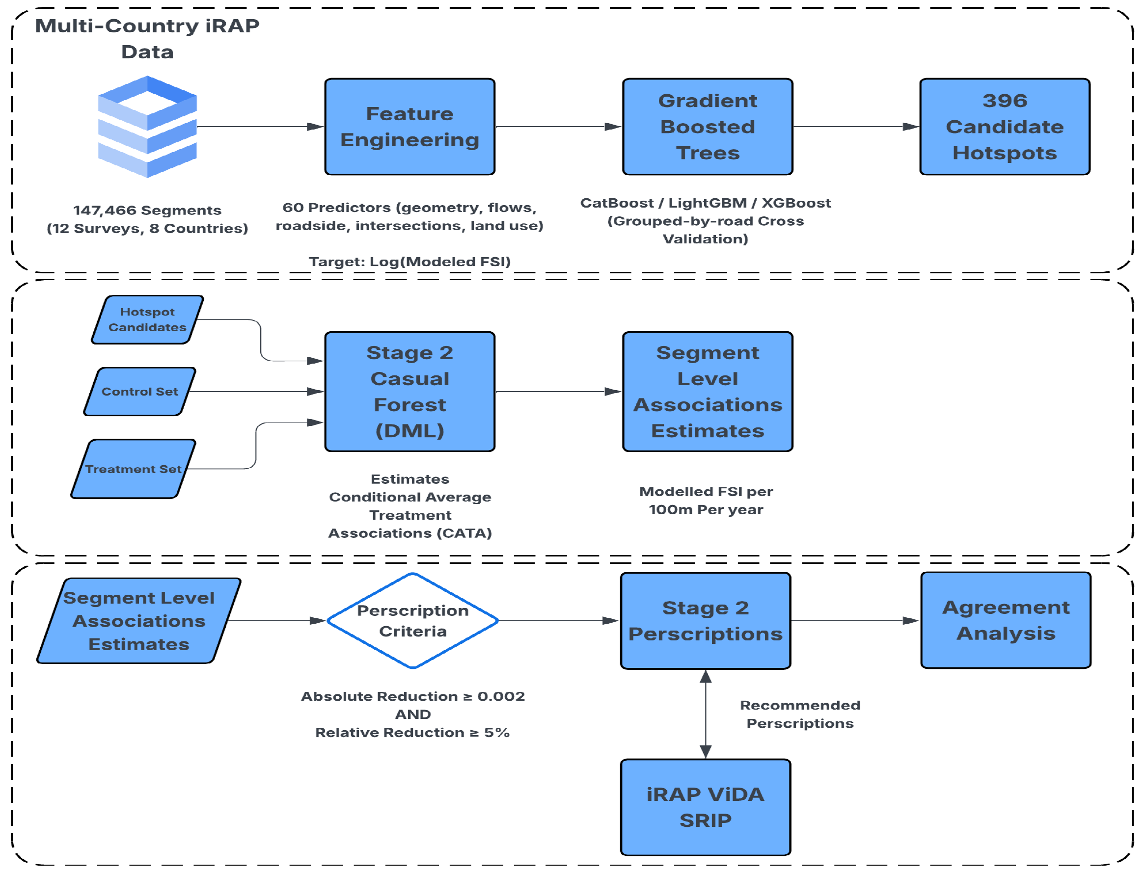
The proposed workflow is illustrated in Figure 1.

2. Related Work

We summarise evidence on heterogeneous safety effects and transferability, review predictive machine learning and causal machine learning in road safety, and position our two-stage audit of ViDA within these strands.

2.1. Crash Modification Factors and Heterogeneous Effects

Crash modification factors (CMFs) have long been used to summarise the expected proportional change in crashes due to specific countermeasures or design changes, and are often reported as single scalar values intended to apply across a wide range of sites. The before–after methodology for isolating such effects was established early [33], and subsequent empirical work has shown that this view is often overly simple. Studies using parametric and nonparametric regression, generalized nonlinear models, and modern tree-based methods have found that the estimated effects of roadside barriers, shoulder width, lane width, and rumble strips depend strongly on context, including traffic volume, speed, roadway class, and crash type [5,6,7,8,23,34]. Recent studies using latent class and discrete outcome models similarly report that built-environment typologies and facility types explain substantial variation in treatment performance, especially for vulnerable road users [35,36,37].
More recent work with generalized random forests and related methods captures this heterogeneity by estimating the conditional treatment effects across covariate profiles [11,23]. Together, this body of evidence suggests that a single CMF per treatment is unlikely to be adequate for targeting interventions and that segment-level or subgroup-specific effects are more informative for planning.

2.2. Transferability, Predictive ML, and Hotspot Detection

A related strand of work questions how well CMFs and safety performance functions (SPFs) transfer to new contexts. Many widely used CMFs originate from high-income countries; applying them without calibration can lead to biased expectations. For instance, Highway Safety Manual models calibrated for multilane rural highways in Saudi Arabia required factors of 0.53–0.78 [38], and transfer-learning studies confirm that naive model transfer degrades performance unless domain shifts are handled carefully [39,40]. Reviews focused on low- and middle-income countries further highlight the scarcity of local evidence and the need for context-specific calibration [3,4]. In this study, we use consistently coded multi-country iRAP data and include dataset identifiers in the Stage 2 control set to absorb survey-level shifts.
Machine learning methods such as random forests, gradient boosting, deep learning, are now widely applied to crash frequency and injury-severity prediction, often outperforming traditional regression [16,17]. Recent extensions address spatial heterogeneity and hotspot identification through learning-to-rank and ensemble approaches [18,19,41]. However, most of this work stops at prediction and ranking; outputs identify high-risk locations but seldom quantify how countermeasures might change risk at specific sites [16,17,20]. Our Stage 1 analysis fits within this prediction-oriented literature (applied to modelled risk outputs rather than observed crashes) and is designed to serve as the input for Stage 2 treatment-association estimation.

2.3. Causal Machine Learning and Heterogeneous Treatment Associations in Road Safety

Causal machine learning methods have recently been adopted in transport safety to estimate the heterogeneous effects of treatments and events. Generalized random forests [42] and causal forests extend tree-based models to estimate conditional average treatment effects (in potential-outcome notation; interpreted here as associations when applied to a deterministic model output) rather than only predicting outcomes, allowing the expected impact of an intervention to vary across covariate space [11,23]. Recent works include simulation-based evaluations of treatment-effect estimators [12] and empirical studies estimating the heterogeneous effects of safety treatments using generalized random forests or causal forests [11,23]. Related work models spatial heterogeneity using other flexible learners, such as geographically weighted neural networks [43].
In parallel, double-robust and double machine-learning frameworks use flexible learners to estimate nuisance functions, such as propensity scores and outcome regressions, and then combine them to obtain effect estimates that are robust to certain forms of model misspecification. Recent applications have studied how different crash types affect traffic [22,25] and investigated the determinants of incident duration [24].
These causal-ML tools complement rather than replace classical econometric heterogeneity models. Random-effects and random-parameter models are designed to capture latent or unobserved heterogeneity in observed crash outcomes [28,29]. By contrast, causal forests partition heterogeneity across observed covariate profiles. In the present study this distinction matters because the outcome is the exported ViDA modelled FSI surface, so Stage 2 targets observed context-specific associations on that surface rather than latent random parameters in observed crash counts.
More generally, methodological overviews emphasise that machine learning and causal inference can be combined to move from pure prediction to heterogeneous treatment-effect estimation and prescription, provided that identification assumptions such as conditional exchangeability and overlap are stated clearly [44].

2.4. Black-Box ML, Explainability, and the Limits of Predictive Importance

The increasing use of machine learning in safety applications has raised concerns regarding the reliance on black-box models for planning interventions. Reviews of explainable artificial intelligence note that post hoc explainers such as SHapley Additive exPlanations (SHAP) can provide insight into model behaviour. However, their attributions depend on the choice of model class, baseline, and feature representation, and they should not be interpreted mechanically as causal effects [20].
Empirical road safety studies using SHAP for pedestrian, truck, and crash severity modelling further illustrate that importance rankings can vary across models and that attributions often reflect correlations rather than actionable effects [45,46,47,48]. Work critiquing feature importance measures likewise shows that different metrics can rank variables very differently and that the importance of prediction does not imply that manipulating a variable would change outcomes in the suggested way [21].
In road safety, review papers warn that high predictive performance alone is not a sufficient basis for designing countermeasure programmes and that machine-learning models are prone to overfitting and temporal instability if not carefully validated [16,17,19,29]. The main implication for the present study is that predictive models and SHAP values should be used to understand how ViDA’s modelled risk surface behaves and to identify hotspots, while formal treatment association work is handled in a separate Stage 2 using causal forests and clear identification assumptions.
Taken together, these strands reveal a clear gap: causal machine learning has begun to enter transport safety [11,22,23,24,25], but it has not yet been integrated with an established infrastructure risk model in a way that supports segment-level prescriptions and benchmarking against the model’s own recommendation engine. Our two-stage framework addresses this gap by combining surrogate modelling and causal-forest association estimation on top of ViDA’s modelled risk surface (see Section 1 for the research questions and contributions).

3. Data

This section describes the multi-country iRAP survey corpus, the ViDA modelled FSI outcome used as the target, and the predictor set used in the two-stage pipeline.

3.1. Study Area, iRAP Surveys, and Reporting Groups

The analysis uses iRAP survey data from twelve projects across eight European countries, obtained through the SENSoR project and the iRAP ViDA platform [13,49]. The combined corpus contains 147,466 unique 100 m road segments. All surveys follow standard iRAP coding protocols for infrastructure attributes and flows [15,50]. We accessed ViDA through a user account to export segment-level FSI and SRIP outputs and did not modify project calibration settings.
Each survey is identified using a Dataset ID. Table 1 summarises the dataset-level segment counts and corpus shares together with the corresponding reporting-group totals and mean modelled FSI. For compact descriptive reporting, we group the 12 surveys into four reporting groups (Table 1). This grouping is used only for descriptive reporting and is not used for model training or estimation. Reporting groups are descriptive survey aggregations, whereas the current grouped analysis uses road labels as the road-level clustering units for validation and cross-fitting. For descriptive context, the current grouped analysis operates on 132 road labels, with a mean length of about 111.7 km and a median length of about 45.8 km. The reporting groups are:
  • EU Central/Adriatic: Dataset IDs 1240, 1242, 1424, 1425, 1426;
  • Western Balkans (non-EU): Dataset IDs 1246, 1247, 12008;
  • EU Southeast Europe: Dataset IDs 1398, 1400, 12983;
  • Eastern Europe: Dataset ID 980.
All modelling is performed on the pooled segment-level dataset.
Table 1 summarises the dataset-level segment counts and corpus shares together with the corresponding reporting-group totals and mean modelled FSI. Mean modelled FSI is reported in units of expected fatalities plus serious injuries per 100 m segment per year. The mean FSI varies across groups, reflecting differences in coded infrastructure, flows, and survey-level calibration within the ViDA engine. In Stage 2, Dataset ID is included as a control to adjust for systematic survey-level differences in the modelled outcome. All subsequent modelling is performed on the full dataset after feature cleaning and removal of variables that are direct outputs of the iRAP risk engine to avoid circularity.

3.2. Outcome Variable: Modelled FSI

The outcome is the ‘Fatal and Serious Injury (FSI) Estimation’ produced by ViDA for each 100 m segment (per year). The ViDA modelled FSI is a calibrated model output. It combines a deterministic, rule-based assessment of infrastructure risk (Star Rating score) and exposure (flow) with a calibration factor. This calibration factor scales the raw risk scores to align them with the fatality totals (or fatality estimates) used in project/network calibration [15]. Consequently, the FSI target represents a modelled expected casualty metric: totals are aligned to project/network fatality totals (or estimates) through calibration, while the spatial distribution is driven by coded infrastructure risk and exposure.

Audit Target and Notation

Let n index road segments. Let X n denote the vector of coded attributes and supporting inputs available in the export (Section 3.3), and let Y n denote the modelling target defined on the log scale. We view ViDA, under fixed project settings and calibration, as an unknown deterministic mapping h such that
Y n = h X n + ε n ,
where ε n captures residual mismatch due to finite coding granularity, export rounding, and unobserved project settings not represented in X n .
Stage 1 fits a surrogate model f ^ of h under road-grouped generalisation. Let g ( n ) denote the road cluster for segment n. Under K-fold grouped cross-validation, we denote by f ^ ( g ) the model trained without any segment from road cluster g and define out-of-fold predictions
Y ^ n , OOF = f ^ ( g ( n ) ) X n .
These Y ^ n , OOF are the only predictions used for hotspot ranking and hotspot-level interpretation.
Stage 2 estimates conditional contrasts on the modelled surface for a restricted treatment action space. For each treatment T k and each binary contrast (e.g., an upgrade from t to t + 1 mapped into T k { 0 , 1 } ), we define
τ k ( x ) = E Y n X n = x , T k = 1 E Y n X n = x , T k = 0 ,
and interpret τ k ( x ) as a conditional association contrast on the calibrated ViDA model output (see Section 1 for how this outcome should be interpreted).
For segment n, the modelled FSI aggregates the expected fatalities and serious injuries across road user groups u and crash configurations c as follows:
FSI n = u c F n , u , c + SI n , u , c
where SI n , u , c is usually derived from fatalities using a default severity ratio
SI n , u , c 10 × F n , u , c
This implies that serious injuries are taken as ten times the number of fatalities unless local crash data are available to support a different ratio [14,15].
The fatality term F n , u , c is itself the output of the iRAP risk model, which combines a road protection score, user-specific flows, calibration factors, and other project settings to yield a modelled number of fatalities for each user–crash type combination on each segment [14,15]. We treat the modelled annual FSI rate per 100 m as the underlying outcome of interest and work with a log-transformed version as follows:
Y n = log FSI n + δ y
where δ y = 10 3 is a small log-offset constant added for numerical stability (to avoid evaluating log ( 0 ) ). Here, log ( · ) denotes the natural logarithm. Exact zero values do occur in the exported segment-level FSI. At the same time, the ViDA FSI target is a continuous modelled expected casualty metric rather than an observed integer crash-count outcome: in our corpus, almost all segment-level values are non-integer. We therefore do not use a Poisson or Negative Binomial likelihood as the main specification [27]. Instead, the log-offset transform handles zeros, compresses the strong right tail, and provides a stable scale for both the Stage 1 surrogate model and the Stage 2 causal forest. All Stage 1 predictive models and Stage 2 causal forests are trained on Y n . Stage 2 associations are estimated on this log scale but are reported as approximate changes in modelled FSI per 100 m per year after back-transformation (see Section 1 for how this outcome should be interpreted).

3.3. Stage 1 Predictors

Stage 1 predictive models use a set of 60 predictors derived from iRAP-coded attributes. These cover traffic exposure, geometry, roadside environment, cross-section, and pedestrian and cyclist facilities. Except for AADT, most flow variables are coded by iRAP as ordered categories (ranges) rather than continuous counts. We exclude all variables that are direct functions of the iRAP risk engine, such as star ratings or intermediate scores, to avoid feeding the outcome back into the predictors. All features were validated for missingness and logical consistency, and categorical variables are recoded to align with the analysis pipelines. Upgrade Cost is included as a context attribute to improve surrogate fidelity, but it is not interpreted as a causal driver of risk or as an intervention lever. The main groups of predictors are as follows:
  • Exposure and flows: Vehicle flow (annual average daily traffic), motorcycle percentage, bicycle and pedestrian flows across the road and along both sides, and observed flows for bicycles, motorcycles and pedestrians.
  • Cross-section and layout: number of lanes, lane width, shoulder presence and quality, median type, carriageway type, and service road presence.
  • Speed and limits: posted speed limits for different vehicle types and operating speed (85th percentile).
  • Roadside and environment: roadside severity object and distance on both sides, land use on both sides, sight distance, skid resistance, and road condition.
  • Pedestrian and cyclist facilities: sidewalks on both sides, pedestrian crossing facilities and crossing quality, fencing, and school zone-related variables.
  • Traffic management and intersections: intersection type and quality, intersection channelisation, speed management and traffic calming, warning signs, and road works indicators.
Table 2 lists candidate predictors and their types (categorical or numerical). Most infrastructure variables follow the iRAP coding manual [26]; Dataset ID is survey metadata, while Upgrade Cost is an iRAP-coded road attribute that captures the relative cost/complexity of major works (land-use/topography) and is used primarily in SRIP costing. As a sensitivity check, we (i) re-estimate Stage 1 without Dataset ID, and (ii) re-estimate Stage 1 under a reduced-information specification that excludes ViDA supporting exposure/speed inputs: Vehicle flow (AADT), Motorcycle %, Bicycle peak hour flow, Pedestrian peak hour flows (across and along both sides), and Operating speed (85th percentile).
The feature engineering pipeline is fully scripted, and each training run stores a feature audit file that records which variables were kept or dropped and why, together with a list of features actually used in the model. This ensures that the exact predictor set for each Stage 1 run can be recovered.

4. Methods

We describe Stage 1 surrogate modelling and SHAP-based interpretation, hotspot selection and diagnostics, Stage 2 treatment-association estimation using double machine learning with causal forests, and the comparison with SRIP recommendations.

4.1. Stage 1 Predictive Modelling and Explanation

The first stage of the framework uses tree-based ensemble models to approximate the iRAP-modelled FSI on a log-transformed scale and to identify high-risk segments for further analysis. Following the data preparation described in Section 3, the target variable is Y n = log ( FSI n + δ y ) for segment n, and the predictor set consists of the Stage 1 predictors in Table 2, including the Dataset ID in the main specification used for hotspot selection and excluding any direct outputs of the iRAP risk engine.
We considered three gradient-boosted tree families that are widely used in crash prediction and injury severity modelling [16,17,32]: CatBoost [51], LightGBM [52], and XGBoost [53]. All models operate on the same training matrix and are evaluated using an identical cross-validation scheme. To avoid spatial leakage and to reflect typical use cases where whole roads are assessed, we use grouped cross-validation by road. All segments belonging to a given named road are assigned to the same fold, and in each iteration, one group of roads is held out as a test set while the models are trained on the remaining roads. This configuration ensures that out-of-fold predictions for each segment are based only on models that have not seen any other segment from the same road.
The hyperparameters for each model family are tuned with a Bayesian Tree-structured Parzen Estimator (TPE) sampler [54], using the mean grouped-by-road cross-validated R 2 as the objective. Each model runs up to 150 trials under the same cross-validation scheme, and the best configuration is then used to generate out-of-fold predictions for all segments. For CatBoost, the search also includes the number of trees and bagging-related parameters, whereas for LightGBM and XGBoost, it explores leaf-wise growth depth and minimum child weight. The selected hyperparameters are listed in Table 3.
The best configuration for each model is then retrained in a cross-validation manner to obtain out-of-fold predictions for all segments. These predictions, together with the true log-FSI values and fold identifiers, are stored in a master file that underpins all diagnostics, hotspot selection, and later analyses. Detailed performance metrics and sensitivity checks are reported in Section 5.1.
Model interpretation in Stage 1 relies on SHAP values [55] computed for the selected CatBoost model on the log-FSI target [20,21]. SHAP provides a local decomposition of the prediction at each segment into feature contributions. To align explanations with the later treatment-association analysis, we compute SHAP values only for the predicted hotspots using out-of-fold models. For each fold, we rank segments within each road by out-of-fold predicted risk, select the top three per road, and compute SHAP values for those segments using the corresponding fold model. We then aggregate the absolute SHAP values across the hotspots to obtain a global feature ranking. These SHAP analyses describe how the predictive model combines infrastructure attributes and flows in high-risk segments, but they are not interpreted as causal effects.

4.2. Hotspot Selection and Diagnostic Ledger

Stage 2 is estimated on the full eligible segment corpus (per-treatment sample size varies after excluding missing values), and association summaries and prescriptions are reported on a small high-risk subset. We define Stage 1 candidate hotspots as the within-road Top-K = 3 segments ranked by Stage 1 out-of-fold predicted log-FSI; this yields 396 hotspots and ensures each road contributes a small set rather than long corridors dominating the subset.
To evaluate Stage 1 as a within-road ranker, we also define a reference hotspot set as the Top-K = 3 segments per road by ViDA modelled FSI on the original scale. We then construct a hotspot overlay ledger that labels segments as true positives (TPs), false positives (FPs), and false negatives (FNs) under two Top-K definitions (reported in Section 5.2). False negatives are retained for diagnostics only. Stage 2 prescriptions and summaries use the 396 candidate hotspots (TP + FP).

4.3. Stage 2 Treatments, Controls, and Identification Assumptions

Stage 2 estimates segment-level associations between actionable infrastructure treatments and the modelled FSI outcome network-wide using a double-machine-learning (DML) causal forest. We report hotspot-level summaries and prescriptions on the Stage 1 candidate hotspots (Section 4.2). The treatment and control sets are defined in the project configuration and checked against hotspot data using simple summary tables of level distributions. Treatments were selected according to the following criteria: actionability, interpretability, and statistical support.
First, a candidate variable must correspond to an infrastructure change that can realistically be implemented as a retrofit on an existing road within the scope of typical safety projects rather than requiring large-scale reconstruction or major land use change. Second, the coding of the variable must have a small number of ordered levels or a binary form so that the contrast is interpretable for engineers. Variables with many unordered categories would require arbitrary collapse, which makes it difficult to map estimated associations to concrete design actions. Third, each level of the candidate treatment must have sufficient representation in the full eligible segment corpus (and also in the hotspot subset for reporting), so that the causal forest does not have to extrapolate into parts of the covariate space with little data. Only six variables satisfy all three criteria, and these form the treatment set in Stage 2. These are:
  • Centreline rumble strips, coded as a binary variable indicating presence versus absence, with the action being the installation or upgrade of strips on undivided roads.
  • Delineation, coded as a binary variable indicating adequate versus poor markings, with the action of repainting or improving markings and posts.
  • Street lighting, coded as a binary indicator of lighting presence, with the action being the installation or upgrade of fixed roadway lighting.
  • Paved shoulder—driver side, coded on a four-level ordinal scale from wide sealed shoulder to narrow, unpaved, or none, with the action being to pave and widen the poor shoulders.
  • Paved shoulder—passenger side, coded on the same four-level ordinal scale for the passenger side.
  • Road condition, coded on a three-level ordinal scale from good to fair to poor pavement, with the action of resurfacing or rehabilitation of poor segments.
Ordinal codes are defined such that lower values represent better conditions (shoulders: 4 worst → 1 best; road condition: 3 poor → 1 good), and Stage 2 targets one-level improvements.
Level-distribution checks confirm sufficient representation for all six variables in both the full corpus and the hotspot subset.
All Stage 2 models adjust for a pre-specified control set of 38 variables covering exposure, geometry, cross-section, roadside environment, pedestrian facilities, intersections, speed environment, and survey metadata. The Stage 1 models were trained on the candidate predictor set as shown in Table 2. For hotspot selection, we use the Dataset-ID-included specification. Sensitivity checks re-estimate Stage 1 (i) without Dataset ID and (ii) under the reduced-information specification, excluding the supporting exposure/speed inputs listed in Table 2. For Stage 2, we define six treatments and a separate set of 38 controls from the cleaned attribute pool, excluding 15 candidate variables after a validation sweep that checked actionability, coding quality, and statistical support. A full list of treatments and controls is provided in Table 4 and Table 5, respectively.
In contrast, some imbalanced but well-defined features are deliberately retained as control variables when they provide important roadway context. For example, shoulder rumble strips are an unbalanced binary code in this sample; nevertheless, their presence is typically characteristic of specific facility types (e.g., rural, higher-speed segments with run-off-road mitigation) and therefore serves as a marker of the broader design and operating environment. We retain this variable as a control to help adjust for systematic differences in road class and cross-section that co-vary with both treatment coding and the modelled outcome. In summary, Stage 2 uses a confounder-rich but quality-screened control set. The feature-classification logic is documented in the code repository.
The modelling strategy follows common assumptions used in causal machine learning, applied here to a deterministic model output. Conditional on the control set, we assume that the treatment codes are not systematically correlated with omitted coded context that also shifts the ViDA modelled outcome and that there is sufficient overlap in treatment prevalence across covariate profiles to support comparisons. We assess overlap using prevalence summaries on the full corpus and on the hotspot subset (Table A1).
In addition, we report treatment-prevalence summaries on the full corpus and on the hotspot subset, and compute treatment-level covariate-balance diagnostics (standardised mean differences for the retained controls). These summaries are used to flag comparisons that rely on weak support and are interpreted conservatively in Section 6. In particular, they help identify contrasts with weaker empirical support, especially where rare treatment levels create limited overlap. Scripts for generating the full prevalence and covariate-balance tables are available in the code repository.
Including Dataset ID as a control helps absorb systematic survey-level shifts, including calibration and other contexts that are constant within a survey. Because the outcome is the ViDA modelled FSI (see Section 1), the causal forest is used to reverse-engineer and audit the effective response surface of the risk model.

4.4. Causal Forest Estimation and Prescription Rule

Stage 2 uses a causal forest [42,56,57] within a double machine learning (DML) framework [58,59], to estimate segment-level conditional average treatment associations for each of the six treatments (Table 4) on the modelled FSI outcome across the full eligible segment corpus. For a given treatment T and outcome Y (the log-transformed modelled FSI), we define a conditional surface contrast on the exported ViDA output:
τ ( x ) = E Y X = x , T = 1 E Y X = x , T = 0 ,
where X denotes the vector of control variables described above.
The outcome Y used in Stage 2 is the actual log-transformed ViDA export, not the Stage 1 prediction. Stage 1 outputs are used only for hotspot definition, hotspot ranking, and hotspot-level interpretation.
For ordinal treatments (paved shoulders and road condition), we estimate adjacent-step contrasts that match a one-level upgrade rule. Specifically, for each ordinal treatment we consider contrasts of the form t t + 1 toward a better code (e.g., shoulders 4 3 , 3 2 , 2 1 ; road condition 3 2 , 2 1 ). We compute these contrasts directly rather than treating the ordinal code as a continuous scalar slope. We denote the resulting segment-level estimates τ ^ ( X ) as conditional average treatment associations (CATA). We use CATA rather than CATE because the outcome is the exported ViDA modelled FSI and the quantity is interpreted as an association contrast on that modelled surface rather than as a causal effect on observed crashes. For each adjacent-step contrast, we restrict estimation to segments whose current code equals either t or t + 1 and define a binary treatment indicator with T = 1 for the better level ( t + 1 ) and T = 0 for level t.
The causal forest is implemented within a double machine learning framework that follows recent work on heterogeneous treatment estimation in transport and related fields [11,22,23,24,25]. For each treatment contrast, we estimate an outcome model g ( X ) using a random forest regressor and a propensity model e ( X ) using a random forest classifier, both with 500 trees, maximum depth 10, minimum leaf size 5, and the square root of the number of features as the splitting subset. Five-fold road-grouped cross-fitting is used, where all segments from the same named road are assigned to the same fold and folds are stratified by Dataset ID so that each fold preserves the survey composition of the full corpus. Orthogonalised outcome and treatment residuals are formed on held-out folds. For the binary adjacent-step treatment contrasts, the propensity score is the out-of-fold predicted probability returned by the random-forest classifier within this grouped cross-fitting procedure. Estimated propensities are trimmed to the interval [ 0.05 , 0.95 ] to stabilise inverse-probability weights in regions of weak overlap. The final-stage causal forest is trained on these residuals together with X, using 1000 trees, maximum depth 8, minimum leaf size 50, and two Monte Carlo iterations. The forest splits on control variables to find regions where the residual association is approximately stable, producing a segment-level association estimate τ ^ n .
Cross-fitting and regularisation inherent to causal forests (subsampling and minimum leaf sizes) mitigate overfitting in heterogeneous association estimation. This procedure is repeated separately for each of the six treatments, with the remaining five treatments and all other covariates used as controls. Therefore, each estimated association is conditional on the current pattern of the other five treatments, and the forest does not attempt to model the joint effect of treatment bundles. The result is a set of six vectors of segment-level associations τ ^ n ( k ) , one for each treatment k, defined on the log-FSI scale. For reporting and decision making, these log-scale associations are converted back to the original FSI scale by applying the inverse of the log transformation at the segment-specific baseline risk. With Y = log ( FSI + δ y ) , a segment-level log-scale association τ ^ corresponds to an implied change on the natural scale of Δ FSI = ( FSI + δ y ) exp ( τ ^ ) 1 .
Road-level empirical Bayes shrinkage.Because roads vary widely in length (and therefore in the number of 100 m segments contributing to each road-level mean), raw segment-level CATA estimates can be noisy for short roads. We stabilise them with an empirical Bayes (James–Stein) shrinkage step. For each road r with n r valid segments, we compute a shrinkage weight w r = n r / ( n r + k ) with k = 20 and pull the road-level mean toward the global mean:
μ ^ r shrunk = w r τ ¯ r + ( 1 w r ) τ ¯ ,
where τ ¯ r is the raw road mean and τ ¯ the global mean. Segment-level deviations within each road are scaled by the same weight: τ ^ n shrunk = μ ^ r shrunk + w r ( τ ^ n τ ¯ r ) . This attenuates estimates for roads with few segments while leaving well-supported roads largely unchanged.
The final step in Stage 2 is to convert the segment-level association estimates into a set of recommended prescriptions. For each hotspot n and treatment k, we use the estimated log-scale association τ ^ n ( k ) and the segment’s baseline FSI to compute an implied change in the modelled FSI per 100 m per year, Δ FSI n ( k ) . We summarise this as an absolute reduction
A n ( k ) = max 0 , Δ FSI n ( k )
and a relative reduction
R n ( k ) = A n ( k ) max FSI n , 10 6 × 100
where the max ( · ) term is used only to avoid division by zero when FSI n = 0 . A treatment k is recommended for segment n if and only if both thresholds are met:
  • A n ( k ) 0.002 fatal and serious injuries per 100 m per year.
  • R n ( k ) 5 % .
These thresholds enforce a minimum practical impact in absolute terms and minimum proportional reduction relative to the segment baseline. The candidate upgrades are triggered only by the absolute and relative reduction thresholds in (9) and (10). Each output consists of a hotspot, a recommended treatment, and the associated estimated change in the modelled FSI.
Uncertainty reporting. Because hotspot retrieval is evaluated under road-grouped generalisation, we use a road-cluster bootstrap for the Stage 1 hotspot retrieval metrics and the Top-K sensitivity analysis. Stage 2 SRIP agreement metrics are reported descriptively in this version.

4.5. Comparison with iRAP ViDA Recommendations

The final part of the methods compares Stage 2 prescriptions with the countermeasures generated by the iRAP ViDA Safer Roads Investment Plan (SRIP) to quantify agreement and to analyse where the two systems diverge. All comparisons are restricted to the six treatment classes defined in Section 4.3.
First, we construct a common representation of the treatments. The iRAP SRIP outputs contain a detailed list of the recommended countermeasures with project-specific labels. To make this comparison, we select SRIP countermeasures that can be mapped to the six treatment classes used in Stage 2. We use the full mapped SRIP export, i.e., the list of technically feasible countermeasures returned by ViDA before later benefit/cost shortlist filtering. This set still reflects SRIP’s built-in feasibility, compatibility, and hierarchy constraints (e.g., spacing rules and treatment hierarchies). By contrast, project-specific discount rates, economic values, and BCR thresholds affect later shortlist formation rather than the segment-level FSI engine itself.
Using a study-specific mapping table, each SRIP countermeasure is assigned to one of the six treatment classes defined in Section 4.3. For example, various forms of line marking upgrade are mapped to delineation, and shoulder surfacing options are mapped to the appropriate paved shoulder treatment. SRIP recommendations that cannot be mapped cleanly to one of these six classes, such as major intersection reconstruction or access management measures, are excluded from the comparison, so that both systems are evaluated in the same treatment space.
Second, we identify an overlapping hotspot set. From the hotspot ledger and the iRAP SRIP outputs, we select 321 Stage 1 candidate hotspots where iRAP has SRIP coverage and at least one SRIP countermeasure can be mapped to our six treatment classes. For each hotspot and treatment, we form two binary indicators: one indicating whether Stage 2 recommends the treatment and another indicating whether SRIP recommends it. If multiple SRIP records map to the same treatment class on the same segment, we set the segment–class indicator to 1 if any record exists (i.e., deduplicate at the segment–treatment-class level). This yields a table with one row per segment and treatment combination, which we use for the classification-style agreement measures.
Agreement between the systems is evaluated on the overlap set using three reported summaries. First, we report prescription-level precision, defined on the segment–treatment label table as the proportion of Stage 2-positive pairs that are also positive in SRIP after mapping and deduplication, i.e., TP / ( TP + FP ) . This is an asymmetric measure conditioned on Stage 2’s recommendations; the complementary quantity conditioned on SRIP (recall) is reported alongside it. Second, we compute Cohen’s κ on the full segment–treatment label table to quantify chance-corrected agreement under the standard definition. Third, we report label-based micro accuracy ( TP + TN ) / N on the same table. Because κ and micro accuracy are computed on the full label table, they include true negatives (pairs where both systems abstain for a given treatment class), and micro accuracy can therefore be influenced by the prevalence of such pairs. We interpret prescription-level precision and kappa as the primary agreement measures and treat micro accuracy as supplementary.
Finally, we use the causal forest output to analyse disagreements in more detail, focusing especially on cases where iRAP recommends a treatment in which Stage 2 declines. For all segment–treatment pairs where SRIP recommends a mapped countermeasure but Stage 2 does not recommend the corresponding class, we extract the corresponding estimated association τ ^ n ( k ) and summarise disagreement patterns by treatment type. This allows us to check whether the causal forest sees these declined interventions as roughly neutral or as potentially harmful in terms of the modelled FSI. A similar exercise can be performed for false positives to determine where the association model recommends treatments that are not present in the SRIP. The combination of prescription-level precision, classification-style agreement, and association summaries provides a structured way to compare rule-based SRIP recommendations with data-driven prescriptions and to ground the discussion in Section 5.5.

5. Results

This section answers the four research questions in sequence: Stage 1 reproduction of the ViDA surface, hotspot retrieval and characteristics, Stage 2 treatment associations, and agreement with SRIP within the mapped six-treatment space.

5.1. Stage 1 Model Performance and SHAP Patterns

Table 6 reports the grouped-by-road cross-validation performance of CatBoost, LightGBM, and XGBoost on the log-transformed modelled FSI outcome.
With the full predictor set, including traffic and vulnerable road user flows and the Dataset ID, CatBoost is the best-performing model, with cross-validated R 2 = 0.916 , mean absolute error (MAE) = 0.241 , and root mean squared error (RMSE) = 0.344 . LightGBM and XGBoost perform slightly worse, with R 2 = 0.899 and R 2 = 0.909 , respectively. LightGBM has MAE = 0.281 and RMSE = 0.394 , while XGBoost has MAE = 0.268 and RMSE = 0.373 . These results indicate that all three gradient-boosted tree models reproduce most of the variation in the ViDA modelled FSI when both infrastructure and flow information are available.
Excluding Dataset ID reduces predictive performance. With flows retained but Dataset ID excluded, CatBoost reaches cross-validated R 2 = 0.878 , mean absolute error (MAE) = 0.281 , and root mean squared error (RMSE) = 0.408 (Table 6). This gap is consistent with Dataset ID capturing survey-level differences such as calibration and other survey-level shifts (e.g., coding or project settings). For hotspot selection we use the Dataset-ID-included CatBoost specification (best predictive fit). Dataset ID is treated as non-actionable metadata and is not interpreted in the SHAP summaries. The high grouped-by-road predictive fit should therefore be read as evidence that the exported inputs recover most of the ViDA segment-allocation pattern, not as evidence of external validity for observed crash outcomes.
When the supporting exposure/speed inputs are removed (reduced-information specification), predictive performance decreases substantially. In this sensitivity run, CatBoost reaches a cross-validated R 2 of 0.438, with an MAE of 0.693 and an RMSE of 0.928. LightGBM becomes the best model in this configuration, with R 2 = 0.442 , an MAE of 0.687, and an RMSE of 0.909, while XGBoost performs slightly worse with R 2 = 0.404 . Even when the Dataset ID is added in the reduced-information configuration, R 2 only increases to about 0.54–0.59 across the three model families, confirming that exposure variables account for a substantial part of the modelled FSI variation and remain more influential than survey-level identifiers. This marked drop helps contextualise the strong all-feature fit by showing that Stage 1 depends materially on the supporting exposure/speed inputs rather than on a trivial restatement of the exported output.
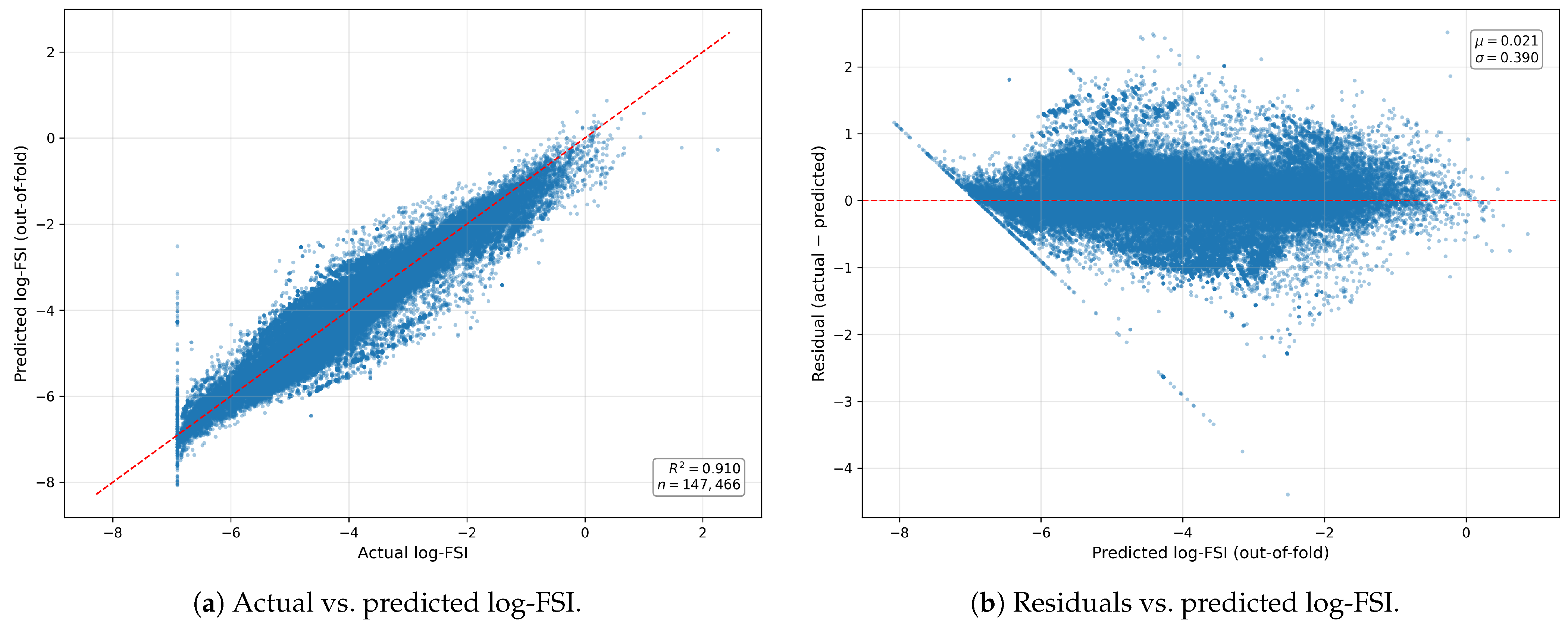
Figure 2 provides a visual summary of the surrogate model fit. The tight clustering around the identity line confirms that the CatBoost model reproduces the ViDA modelled FSI with high fidelity across the full range of segment-level risk values. The residual plot (Figure 2b) shows no fan-shaped pattern, confirming homoscedastic prediction errors across the risk spectrum.
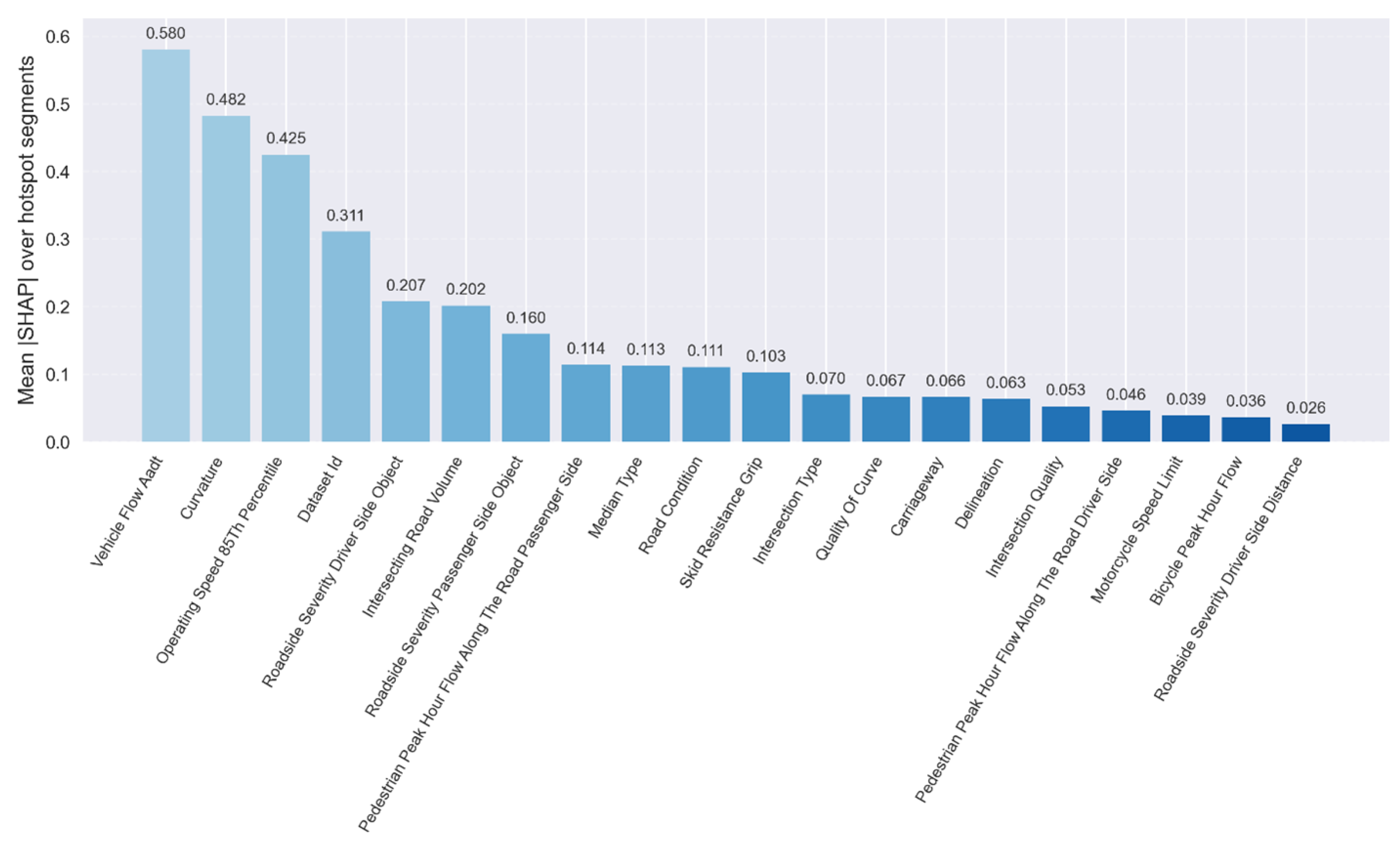
Figure 3 shows the mean absolute SHAP values for the selected CatBoost model on the predicted hotspots, highlighting the main predictors of modelled risk at high-risk segments. For each hotspot, SHAP values are computed using the out-of-fold model and then aggregated across all hotspots to obtain a global ranking.
Inspection of the signed SHAP distributions for the top features shows clear directional patterns. Figure 3 indicates that Vehicle flow (AADT) and Dataset ID are the strongest predictors on the hotspot set, reflecting the exposure-weighted structure of the ViDA FSI outcome and survey-level shifts across datasets. Because these variables are non-actionable, we focus interpretation on the highest-ranking infrastructure attributes: operating speed, curvature, shoulder condition, delineation, lighting, and roadside severity. Higher operating speeds and tighter curvature are associated with positive SHAP contributions to the log-FSI prediction (higher modelled risk), whereas wider paved shoulders, better pavement condition, adequate delineation, and the presence of lighting are associated with negative contributions. Pedestrian and cyclist flows and facilities also appear prominently among the top features, reflecting the importance of vulnerable road user exposure on many hotspots. These patterns are consistent with engineering expectations under the iRAP protocols, but they remain purely predictive descriptions of Stage 1 model behaviour on the hotspot set.

5.2. Hotspot Characteristics and Spatial Patterns

The Stage 1 hotspots are spread across all 12 surveys and all four reporting groups, so every reporting group contributes roads with segments in the highest modelled risk band rather than risk being concentrated in a single country or network.
Hotspots are predominantly located on roads with higher operating speeds and more demanding geometries, consistent with the SHAP patterns in Section 5.1, but also include some urban and peri-urban links where vulnerable road user flows are high. Summaries compiled from the hotspot ledger and underlying segment dataset show that each reporting group has a mixture of hotspot road classes rather than a single dominant class.
The hotspot ledger described earlier underpins all the hotspot-level analyses in this section. It contains 499 segments: 293 where the Top-3-per-road sets by Stage 1 out-of-fold prediction and by ViDA modelled FSI agree (true positives), 103 false negatives, and 103 false positives. The 396 Stage 1 hotspots used in Stage 2 are the union of the true positives and false positives, whereas the full 499-row ledger is retained for quality assurance and diagnostic checks. Here, predicted refers to Top-K by Stage 1 out-of-fold prediction, while actual refers to the reference Top-K defined by ViDA modelled FSI on the original scale. Table 7 reports the hotspot retrieval metrics under the two Top-K definitions.
To quantify sampling variability under road-level clustering, we also report road-cluster bootstrap confidence intervals for the Table 7 metrics. Bootstrap resampling is performed at the road level to preserve within-road dependence.
To assess the robustness of hotspot retrieval to the definition width, we sweep K { 1 , 3 , 5 } and report road-cluster bootstrap confidence intervals (Table 8). Cohen’s κ ranges from 0.697 at K = 1 to 0.760 at K = 5 , and all three confidence intervals overlap substantially. Even at K = 1 (the hardest task: identifying the single riskiest segment per road), agreement exceeds the Landis–Koch “substantial” threshold ( κ > 0.61 ). The gentle monotonic increase reflects a mathematical property (selecting more segments per road increases the opportunity for overlap) rather than model instability. We retain K = 3 as the operational choice.

5.3. Stage 2 Treatment Associations

We now summarise the causal-forest association estimates on the predicted hotspots for the six treatments, together with their baseline prevalence.
The treatment prevalence in the full corpus supports estimation, and the prevalence in the hotspot subset supports hotspot-level summarisation and prescriptions. Street lighting is present in 51.8% of hotspots, while centreline rumble strips are present in 35.4% (Table 9). Shoulder conditions are heavily skewed toward the worst levels on both sides, with most hotspots having narrow or no paved shoulders. These patterns support the interpretation of shoulder-related prescriptions as upgrades from common poor states to better-engineered cross sections (Table 9). Here prevalence refers to the baseline coded treatment status (e.g., lighting present vs. absent), not to SRIP recommendations. This caution is most relevant for the rarer upper shoulder levels on the hotspot subset. For example, Table 9 shows only 1 hotspot in the wide driver-side shoulder state and 7 in the medium driver-side shoulder state, so these contrasts should be interpreted more cautiously than the more prevalent binary treatments.
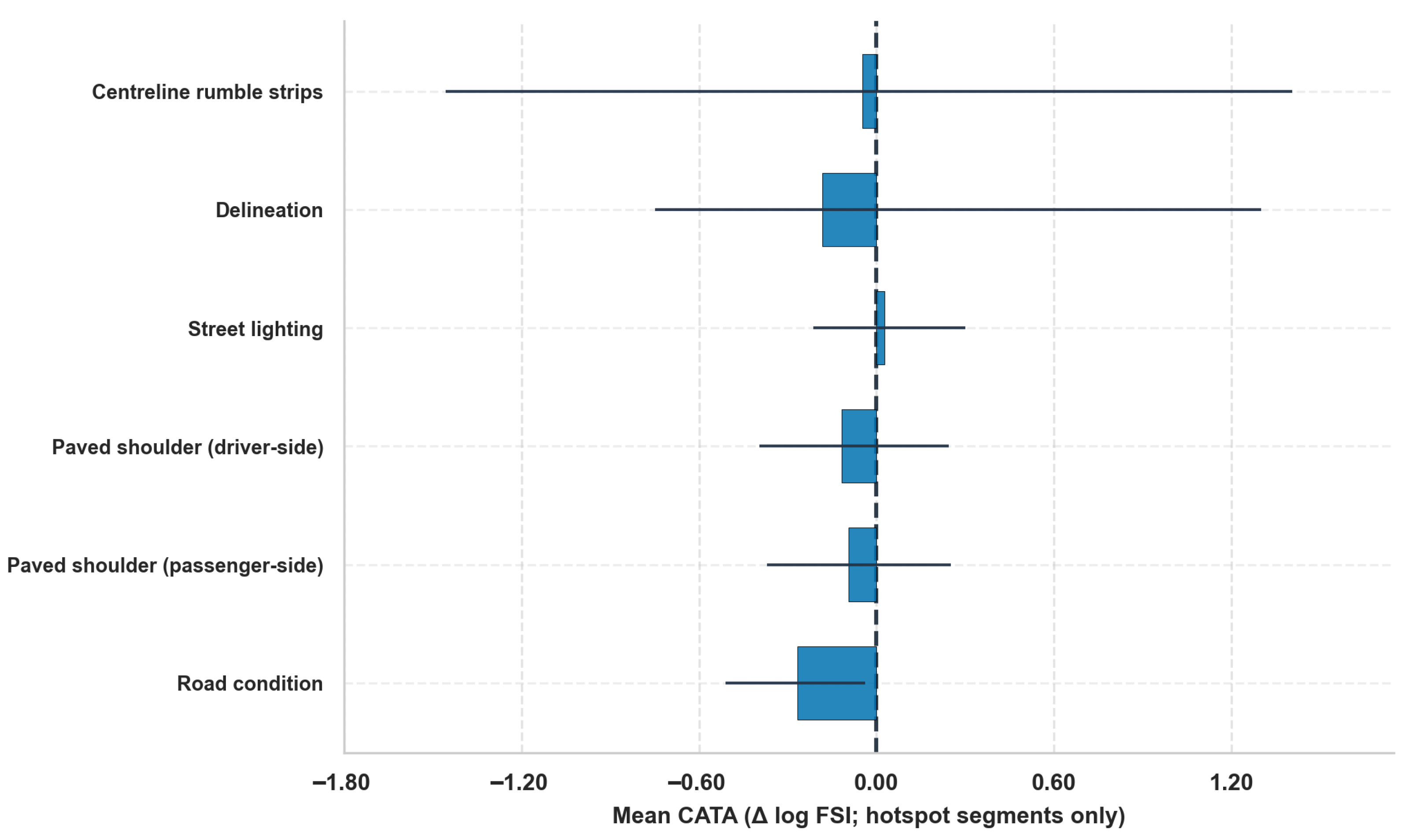
Causal forest estimates reflect these prevalence patterns. For each treatment and hotspot, we obtain an estimated association on the log-FSI scale and convert it to an implied change in the modelled FSI per 100 m per year. Negative associations (and negative implied Δ FSI after back-transformation) correspond to lower modelled FSI and are interpreted as beneficial within the ViDA modelled risk surface. Figure 4 summarises these associations over all hotspots. The mean associations are small in magnitude for all six treatments, and the percentile ranges include both negative and positive values. Overall, no treatment delivers a large, uniform reduction in the modelled FSI when averaged over the full hotspot set. Instead, there is substantial heterogeneity, with a minority of hotspots exhibiting sizable negative associations and many hotspots showing near-neutral or mildly positive associations. This pattern is consistent with the heterogeneous CMF literature reviewed in Section 2, which emphasises that the association of a given intervention depends on the local combination of geometry, flow, and roadside environment (e.g., [5,7,11,33]).
These association patterns provide an internally consistent view of where each standard treatment appears the most promising in terms of reducing the modelled FSI within the iRAP framework.

5.4. Stage 2 Prescriptions

The quantities reported in this subsection are association-based candidate upgrades on the ViDA modelled FSI surface, not direct estimates of observed crash effects. Applying the prescription rule in Section 4.4 yields 1170 actionable candidate upgrades across the 396 hotspots (Table 10); only 362 of the 396 hotspots receive any Stage 2 prescription (34 have none). The largest groups are paved shoulder upgrades (driver side: 177 + 104 + 6 = 287; passenger side: 143 + 87 + 11 = 241), delineation improvements (220), and pavement rehabilitation (road condition: 107 + 136 = 243). Installation upgrades are also common for centreline rumble strips (129) and street lighting (50).
Table A3 shows that prescription counts and actionable upgrades are stable over a reasonable range of threshold values.
Therefore, this candidate-upgrade set is the result of a combination of three elements: the learned risk surface from Stage 1, estimated treatment associations from the causal forest, and decision thresholds that encode a minimum practical benefit. This structure differs from traditional CMF-based planning, where a single effect size is applied uniformly, and instead moves toward a heterogeneous association/sensitivity view in which treatments are favoured on segments where they are expected to have larger relative or absolute benefits [6,23].
These patterns align with the baseline distributions in Table 9: approximately 70% of hotspots have poor delineation, and most hotspots have narrow or no paved shoulder on each side. Most shoulder upgrades are stepwise (code 4→3, code 3→2), whereas upgrades to wide shoulders (≥2.4 m) are rare (Table 10).
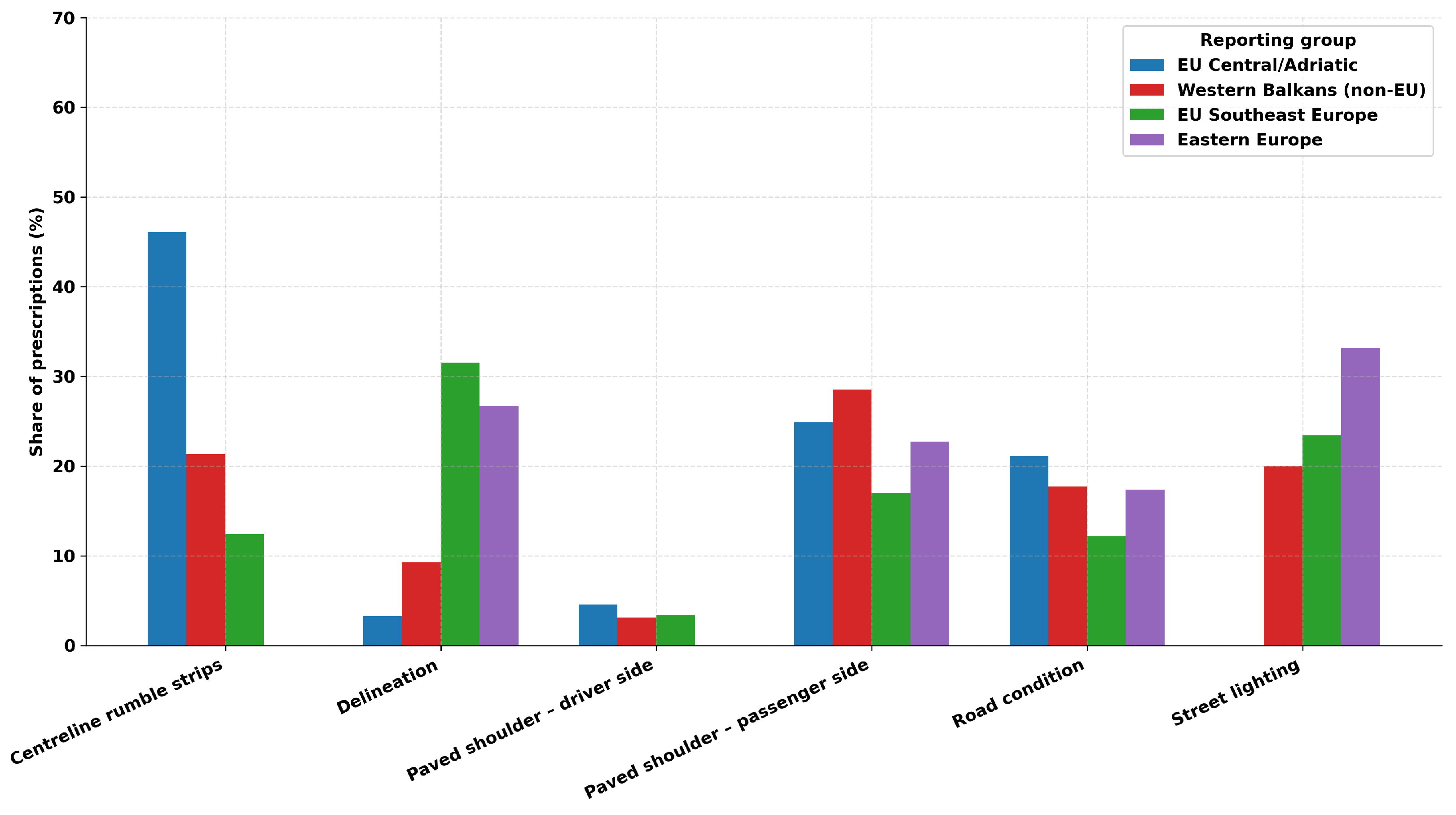
Figure 5 summarises the reporting-group mix of Stage 2 prescriptions. Western Balkans (non-EU) are dominated by centreline rumble-strip prescriptions, whereas EU Southeast Europe and Eastern Europe show a larger share of delineation and cross-section upgrades (paved shoulders and road condition). The EU Central/Adriatic exhibits a more balanced prescription set with comparatively higher road-condition and delineation upgrades. Street lighting remains a small share across the groups. Code definitions follow the iRAP coding manual [26].
The full prescription ledger provides segment-level details of every prescribed treatment, including the baseline modelled FSI and the estimated change. These outputs are used in Section 5.5 to compare the model-based prescriptions with the iRAP ViDA SRIP recommendations.

5.5. Agreement and Disagreement with iRAP ViDA

To compare the Stage 2 prescriptions with the iRAP ViDA Safer Roads Investment Plan, we focus on the subset of hotspots where both systems operate in the same treatment space.
Using the mapping procedure described in Section 4.5, we identify 321 overlap hotspots with SRIP coverage and at least one mapped countermeasure in the six-treatment space (Table 11). On this overlap set, we construct a binary segment–treatment label Table (321 × 6 pairs) after deduplicating SRIP at the segment–treatment-class level. In this table, Stage 2 and SRIP agree on 712 segment–treatment pairs where both recommend the same class (TP). Stage 2 recommends an additional 360 pairs that SRIP does not (FP), while SRIP recommends 217 pairs that Stage 2 does not (FN), and both abstain on 637 pairs (TN). This yields a prescription-level precision TP / ( TP + FP ) = 0.664 , micro accuracy ( TP + TN ) / N = 0.700 , and Cohen’s κ = 0.403 (Table 11). Because the marginal recommendation rates are high on this overlap set, chance agreement is also substantial enough to matter. This is why Cohen’s κ is informative alongside precision and recall. The observed agreement of 0.70 should therefore be read against an expected agreement of roughly 0.50 from the marginals alone, which is consistent with the reported κ of about 0.40.
To localise where the two systems agree and diverge, we decompose the 321   ×   6 label table by treatment class (Table 12).
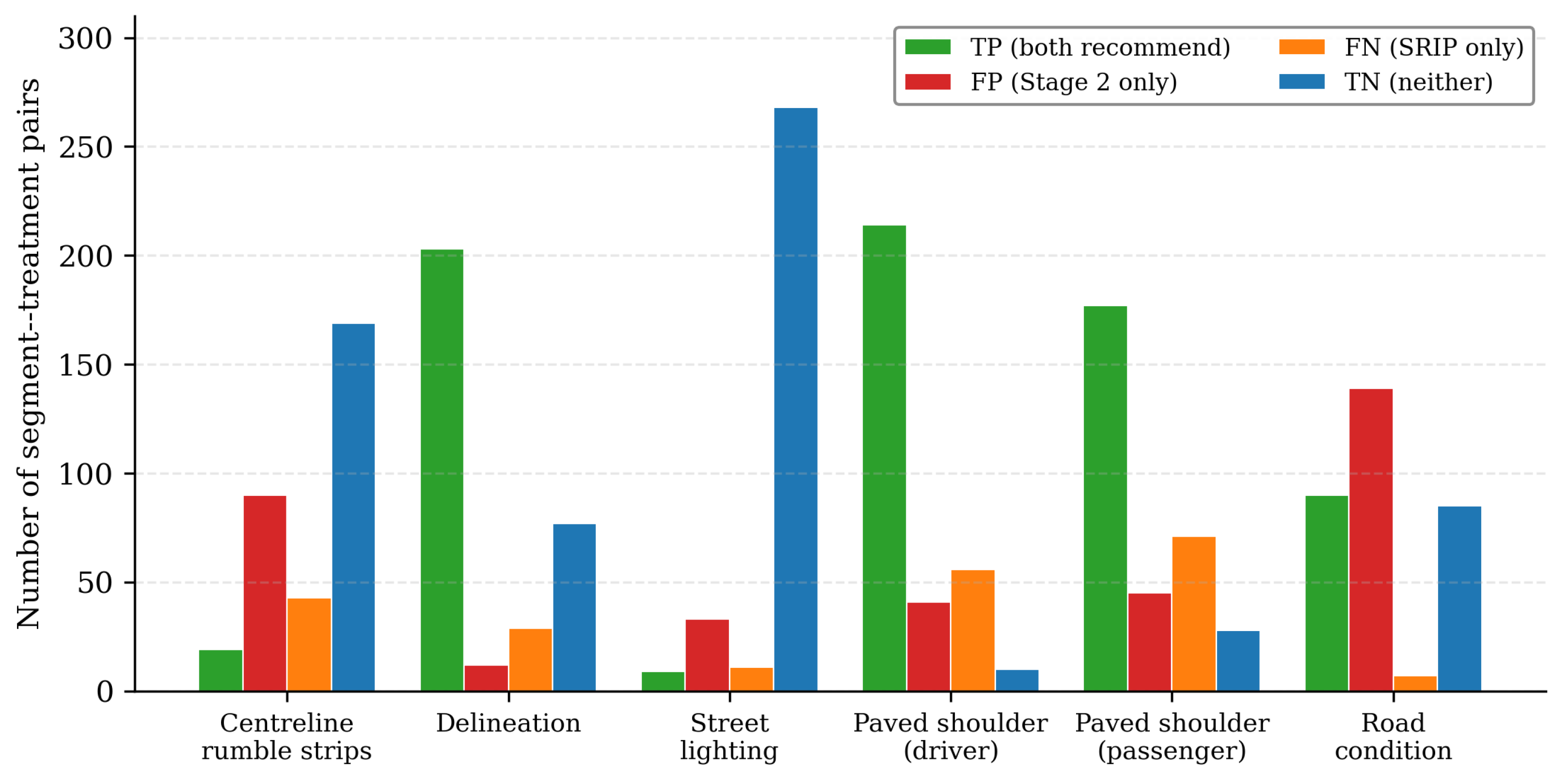
Figure 6 provides a visual decomposition of the per-treatment confusion counts.
Delineation dominates agreement ( κ = 0.70 ; precision 0.94), meaning both systems almost always concur on whether a segment needs improved road marking. Paved shoulders (driver and passenger) show high precision but near-zero κ : both systems recommend these treatments on roughly 80% of overlap segments, so most matches are expected by chance alone and κ registers no above-chance agreement despite the high raw hit rates. Centreline rumble strips and street lighting exhibit the lowest precision (0.17 and 0.21), indicating that Stage 2 prescribes these treatments much more broadly than what SRIP maps, a pattern that may reflect either SRIP mapping gaps or associations that the causal forest detects but that SRIP’s rule triggers do not capture. Road condition has the highest recall (0.93) yet modest precision (0.39): nearly every SRIP recommendation is echoed, but Stage 2 also flags 139 additional segments.
This moderate aggregate overlap ( κ = 0.40 ) indicates that the causal-forest-based system and rule-based SRIP logic often propose different treatments at the same hotspots, even when they operate on the same segments and the same six treatment classes. It does not, by itself, indicate which system is correct, but it motivates a closer examination of the direction of disagreements. Because micro-accuracy is sensitive to the prevalence of no-recommendation cases at the segment–treatment level, we emphasise prescription-level precision and Cohen’s κ as the main agreement measures (Table 11 and Table 12). To analyse disagreements, we focus on SRIP-only recommendations (pairs where SRIP recommends a mapped countermeasure but Stage 2 does not) and summarise the corresponding estimated associations by treatment type. In practice, these disagreement cases are the main audit value of the comparison because they identify sites where rule-based triggers and data-driven associations diverge and therefore merit closer engineering review.
For each segment and treatment where SRIP recommends a countermeasure and Stage 2 does not, we retrieve the corresponding estimated association and summarise its distribution by treatment type. Disagreements remain within the mapped six-treatment space (FP = 360 and FN = 217; Table 11). Because SRIP is a rule-based engineering system (with feasibility triggers, hierarchies, and spacing constraints) and Stage 2 estimates segment-level associations on the modelled risk surface, differences can reflect both the method and definition/mapping choices rather than a clear error by either system.
From the perspective of the causal forest, many SRIP-only recommendations have estimated associations that are small or even adverse on the modelled risk surface. SRIP logic encodes fixed risk-reduction assumptions for these treatments, so positive associations may reflect residual confounding where the treatment serves as a proxy for unobserved risk factors in the dataset that the control set could not fully absorb. This is consistent with the broader literature on heterogeneous treatment effects and CMFs, which shows that pooled effect estimates can obscure subgroups where benefits are limited or negative [5,11,23,33].
The false-negative analysis suggests a divergence in estimated safety association: SRIP identifies these actions as feasible interventions expected to reduce modelled risk, whereas the causal forest estimates that, conditional on the local covariate profile, these actions are associated with no reduction or a slight increase in modelled FSI. This highlights the systematic difference between ViDA’s rule-based protocols and the data-driven associations learned from this dataset.

6. Discussion

We first interpret the main findings in the context of the ViDA audit, then relate the results to the broader CMF heterogeneity and transferability literature, discuss implications for integrating ML and causal ML into road safety practice, and acknowledge limitations.

6.1. Interpretation of the Main Findings

This study aimed to learn from and augment an existing infrastructure risk model rather than replace it. The central motivation is that ViDA’s modelled FSI, although deterministic at the segment level, is anchored to project- or network-level fatality totals or fatality estimates used in calibration. A data-driven surrogate can therefore reveal whether the deterministic allocation rules distribute this calibration-anchored risk in ways that are consistent with known infrastructure–crash relationships, or whether they introduce systematic patterns that pure rule inspection would not expose. The DML framework serves this audit function by adjusting for correlated road context. It isolates what the modelled risk surface attributes to each treatment and provides a structured comparison against the global CMFs embedded in iRAP’s SRIP logic.
In Stage 1, the surrogate reproduced the ViDA risk surface with high accuracy under grouped-by-road cross-validation ( R 2 0.92 with flows and Dataset ID). The marked performance drop when flows were removed confirms the central role of exposure in the ViDA computation. SHAP analyses on the hotspot subset showed that the surrogate distributes attributions consistently with the iRAP coding logic: speed, curvature, shoulder quality, delineation, lighting, and roadside hazard severity are the leading contributors, in directions that match engineering expectations.
In Stage 2, the causal forest revealed that treatment associations vary in both sign and magnitude across hotspots. No single treatment delivers a large, uniform reduction. Instead, a minority of segments exhibit sizeable negative associations while many show near-neutral values. The resulting candidate upgrades (Table 10) favour centreline rumble strips and delineation on high-speed undivided roads and are more selective for shoulders and pavement, appearing mainly at the worst-coded segments.
Comparing these candidate upgrades with iRAP’s SRIP shows partial alignment within the mapped six-treatment space (Table 11 and Table 12). Because SRIP is a rule-based protocol with feasibility constraints and a wider intervention catalogue, disagreements reflect differences in objective function, mapping detail, and road context rather than implying that either system is wrong. The results support the view that a causal forest layered on top of the ViDA surface can highlight where standard treatments appear most promising or questionable in terms of modelled FSI, complementing rule-based guidance with data-driven evidence.

6.2. Relation to CMF Heterogeneity and Transferability Literature

The heterogeneous treatment associations and moderate prescription-level precision are consistent with the broader literature on CMF and transferability. Studies have shown that the impacts of roadside barriers, shoulders, lane width, shoulder width and related design elements vary with traffic volume, curvature, speed regime and crash type [5,7,8,33], and recent work with generalized random forests and causal forests makes this heterogeneity visible [11,23].
In our results, only a subset of hotspots receive prescriptions for any given treatment, even where poor conditions are common, and prescription mixes differ across reporting groups, mirroring evidence that not all poor segments are equally good candidates and that effect sizes can vary across countries and networks [3,4]. Against this backdrop, partial agreement with SRIP on overlapping hotspots is unsurprising: a globally calibrated expert system and a data-driven model calibrated to a specific multi-country dataset will sometimes diverge, including cases where the causal forest estimates near-zero or positive associations for SRIP-only recommendations.
This pattern is consistent with how SRIP and data-driven association models differ in design and calibration. iRAP applies globally calibrated engineering rules with feasibility triggers, hierarchies, and compatibility constraints, and SRIP outputs can later be filtered by the benefit/cost ratio in standard workflows (not applied in our comparison). In contrast, causal forest estimates segment-level associations within a specific multi-country dataset. From a transferability perspective, it is expected that an expert system designed to be globally applicable will sometimes diverge from a data-driven system calibrated to a particular set of networks, even when they share the same underlying infrastructure coding. The small or positive associations for some SRIP-only recommendations suggest that part of this divergence reflects rule-based recommendations being applied in contexts where local conditions make the expected benefit small, a phenomenon that the heterogeneous CMF literature has emphasised.

6.3. Implications for Using ML and Causal ML in Road Safety Practice

Reviews of crash prediction and explainable AI note that tree-based and boosting models often outperform traditional regression for prediction but warn that feature importance and SHAP-type attributions describe model behaviour rather than treatment effects and can be sensitive to modelling choices [16,17,20,21,32]. By separating predictive Stage 1 from association-focused Stage 2, the framework aligns with this guidance: Stage 1 uses machine learning and SHAP to reproduce and interpret the exported iRAP modelled risk surface and to test hotspot recovery under road-grouped validation, while Stage 2 uses a causal forest with explicit control sets and identification assumptions to estimate conditional treatment associations on the actual ViDA outcome.
This choice is specific to the task in this paper. Stage 1 is not a conventional crash-count regression problem. It is an audit task that asks whether the exported ViDA surface can be reconstructed from many mixed-type coded inputs. Stage 2 is not designed to estimate one global treatment coefficient. It allows treatment associations to vary across observed road contexts on a continuous modelled outcome surface. Classical regression, mixed, and random-parameter models remain important, especially for observed crash outcomes [27,28,29,60], but they answer a different question from the present ViDA-audit task.
In practice, model-based methods can be layered on top of iRAP as an additional auditing lens on where and how to act, rather than as a replacement for engineering judgement or benefit/cost analysis [11,22,23,24,25].
The most practical workflow is to use the framework after a standard ViDA assessment, not instead of it. Agencies would first obtain the usual segment-level FSI and SRIP outputs, then use Stage 1 to check how strongly the exported coding and supporting inputs reproduce the resulting hotspot pattern. Stage 2 then adds a context-sensitive review layer for the six mapped treatment classes on the high-risk subset. The most decision-relevant cases are those where Stage 2 and SRIP disagree because these segments warrant closer engineering review rather than automatic acceptance of either output. Where treatment support is weak, interventions fall outside the mapped treatment set, or cost and constructability dominate the decision, SRIP and engineering judgement should remain primary.

6.4. Limitations and Directions for Future Work

This study had several limitations. First, the outcome is ViDA’s modelled FSI, not segment-level observed crashes. The FSI totals are anchored through project/network calibration to fatality totals or fatality estimates, but the segment-level allocation is rule-based given the coded inputs and project settings. The associations estimated in Stage 2 therefore audit how the ViDA risk surface responds to coded treatments under adjustment for correlated context, and they are not a substitute for validation against observed crash outcomes.
Second, Stage 2 relies on observational variation in treatments across the full eligible segment corpus. We summarise and prescribe the resulting associations on the hotspot subset and rely on a conditional exchangeability assumption given the control set. Even with rich controls and dataset identifiers (encoded as survey dummies), residual confounding is likely, especially where treatments are targeted at the worst sites or data quality varies across networks. Dependence is partly addressed through grouped-by-road validation in Stage 1, grouped-by-road cross-fitting in Stage 2, and a road-level shrinkage step, but it does not explicitly model spatial autocorrelation among adjacent segments or a full multilevel segment-road-survey hierarchy. Individual segment-level association estimates can be noisy, especially for rare treatment levels or weak overlap. Prescriptions should therefore be treated as candidates for engineering review rather than precise effect estimates. The balance and prevalence diagnostics are intended as transparency checks, not as proof that exchangeability holds. The causal forest captures heterogeneity conditional on observed coded covariates. It does not model latent random parameters or other forms of unobserved heterogeneity in the way random-parameter crash models do [28,29].
Third, the analysis is limited to six retrofittable treatments and a fixed prescription rule based solely on absolute and relative reductions in the modelled FSI. Other potentially important interventions, such as access management, intersection redesign, and enforcement measures, are present in the data but were excluded because of concerns about clear practical meaning, interpretability, or adequate support in the data. The thresholds for issuing prescriptions are illustrative defaults; prescription counts are stable across a threefold range of both parameters (Table A3), but different agencies could adopt context-specific thresholds or embed associations in formal budget allocation models. Stage 2 does not account for costs, whereas SRIP can incorporate benefit/cost ratios in standard workflows (not applied in our comparison).
Fourth, the dataset comprises 12 surveys conducted in eight European countries, featuring a diverse mix of road types, traffic conditions, and calibration practices. This provides more diversity than a single-country study but still represents a specific set of contexts. Extending the analysis to additional regions, especially low- and middle-income countries with different infrastructure and user mixes, is required to test robustness and generality.
Finally, the results depend on modelling choices: the selection of gradient-boosted trees and causal forests, tuning of these models, hotspot definition, and trimmed feature set used in Stage 2. We intentionally retain six treatments and 38 controls and exclude 15 variables that were ill-defined, extremely sparse, or duplicated to avoid unstable encodings, but this may leave some policy or contextual factors only partially captured in the retained control set.
Therefore, future studies should focus on the following directions. First, linking modelled-FSI-based prescriptions to observed crash or injury outcomes over time, to examine whether hotspots with strong negative associations indeed experience larger crash reductions after treatment. Second, exploring alternative causal estimators and sensitivity analyses, including methods that directly assess the impact of unobserved confounding. Third, integrating the association estimates into budget-constrained optimisation models and operational decision-support tools that can be used alongside iRAP in project preparation and network screening.

7. Conclusions

Using multi-country ViDA outputs for 147,466 segments, we developed a two-stage framework that combines gradient-boosted surrogate modelling (Stage 1) with causal-forest double machine learning (Stage 2) to audit the iRAP modelled FSI surface. Stage 1 reproduced most of the variation in modelled FSI under road-grouped cross-validation, with operating speed, curvature, shoulders, delineation, and lighting as leading contributors. Stage 2 estimated segment-level treatment associations for six retrofit interventions and, after applying simple reduction thresholds, produced 1170 association-based candidate upgrades on 396 hotspots. Comparison with iRAP’s SRIP recommendations within the same six-treatment space shows partial agreement (Recall = 0.77, Precision = 0.66, κ = 0.40 ) alongside structured divergence that motivates targeted engineering review.
The framework provides (i) a transparent statistical audit of how modelled FSI varies with coded infrastructure and flows, (ii) heterogeneous, code-level candidate upgrades derived from conditional associations, and (iii) a structured comparison against SRIP that highlights where the two systems converge and diverge. For agencies already using iRAP, it offers a way to add data-driven evidence on existing practices: identifying where treatments appear most promising, flagging interventions that merit closer review, and informing validation studies. Linking these candidate upgrades to observed crash outcomes, expanding the treatment set, and embedding associations in budget-constrained decision processes are the key next steps.

Author Contributions

Conceptualization, A.H. and B.A.; methodology, A.H.; software, A.H.; validation, B.A., M.S. and M.Š.; formal analysis, A.H.; investigation, A.H.; resources, M.Š.; data curation, A.H.; writing—original draft preparation, A.H.; writing—review and editing, B.A., M.S. and M.Š.; visualization, A.H.; supervision, B.A. and M.Š.; project administration, A.H.; funding acquisition, M.Š. All authors have read and agreed to the published version of the manuscript.

Funding

This project has received funding from the European Union’s Horizon Europe research and innovation programme under grant agreement No 101119590. UK participants in Horizon Europe Project IVORY are supported by UKRI grant numbers EP/Y036026/1 (The International Road Assessment Programme—iRAP) and EP/Y036034/1 (Agilysis).

Data Availability Statement

Data were obtained from iRAP ViDA and are available subject to iRAP licensing terms. The analysis code is available at https://github.com/AmirHHasani/irap-vida-fsi-audit, (accessed on 1 March 2026).

Acknowledgments

During the preparation of this manuscript, the authors used ChatGPT-4o for the purpose of refining and enhancing the clarity of the writing. The authors have reviewed and edited the output and take full responsibility for the content of this publication. We confirm that the results are accurate within our experimental settings.

Conflicts of Interest

The authors declare no conflicts of interest. The funders had no role in the design of the study; in the analyses, or interpretation of data; in the writing of the manuscript; or in the decision to publish the results.

Appendix A. Treatment Prevalence Checks

Table A1. Treatment prevalence on the eligible segment corpus, by treatment and coded level. Counts and shares are computed over non-missing values; N non - missing = 147 , 466 for all treatments shown.
TreatmentLevel (Code Meaning)CountShare
Centreline rumble stripsAbsent (code 1)119,56081.1%
Centreline rumble stripsPresent (code 2)27,90618.9%
DelineationAdequate/good (code 1)97,79466.3%
DelineationPoor (code 2)49,67233.7%
Street lightingNot present (code 1)90,78861.6%
Street lightingPresent (code 2)56,67838.4%
Paved shoulder–driver sideWide (≥2.4 m, code 1)18021.2%
Paved shoulder–driver sideMedium (1 m to <2.4 m, code 2)72754.9%
Paved shoulder–driver sideNarrow (0 m to <1 m, code 3)89,96861.0%
Paved shoulder–driver sideNone (code 4)48,42132.8%
Paved shoulder–passenger sideWide (≥2.4 m, code 1)23,31715.8%
Paved shoulder–passenger sideMedium (1 m to <2.4 m, code 2)24,60116.7%
Paved shoulder–passenger sideNarrow (0 m to <1 m, code 3)51,74035.1%
Paved shoulder–passenger sideNone (code 4)47,80832.4%
Road conditionGood (code 1)95,10764.5%
Road conditionMedium (code 2)38,18725.9%
Road conditionPoor (code 3)14,1729.6%

Appendix B. Road Condition Step-Contrast Check

Table A2. Ordinal step-contrast check for Road condition. For each contrast, models are trained on the full eligible segment corpus and summaries are reported on the 396 candidate hotspots (TP + FP) restricted to the contrast subset. Mean baseline FSI and mean Δ FSI are reported on the natural scale (FSI per 100 m-year); mean relative change is computed as 100 × Δ FSI / FSI .
ContrastHotspots (N)Baseline FSI Δ FSI Rel. Change (%)
3→2 (Poor→Medium)1140.329 0.084 25.4
2→1 (Medium→Good)1400.312 0.074 23.8

Appendix C. Prescription Threshold Sensitivity

Table A3. Sensitivity of prescription volume to the absolute (A) and relative (R) reduction thresholds on the hotspot population. Total prescriptions counts all recommended (segment, treatment) pairs after thresholding; actionable upgrades counts only recommendations that change the current code (no-change validations excluded).
ARTotal (N)Upgrades (N)Hotspots (N)
0.0012.517651267375
0.0015.016761208374
0.00110.014501020359
0.0022.516991224363
0.0025.016171170362
0.00210.01395986349
0.0042.515891161348
0.0045.015311119347
0.00410.01316939335

References

  1. World Health Organization. Global Status Report on Road Safety 2023; Technical Report; World Health Organization: Geneva, Switzerland, 2023; Available online: https://www.who.int/publications/i/item/9789240086517 (accessed on 1 March 2026).
  2. World Bank. iRAP Impact Evaluation the UNRSF Ten Step Plan for Safer Road Infrastructure in Improving the Safety Performance of WB Projects (P175118); Technical Report; World Bank Group: Washington, DC, USA, 2024; Available online: https://documents1.worldbank.org/curated/en/099040124131514284/pdf/P1751181bcc609021a3f01dbabdc604b95.pdf (accessed on 1 March 2026).
  3. Tavakkoli, M.; Torkashvand-Khah, Z.; Fink, G.; Takian, A.; Kuenzli, N.; de Savigny, D.; Muñoz, D.C. Evidence From the Decade of Action for Road Safety: A Systematic Review of the Effectiveness of Interventions in Low and Middle-Income Countries. Public Health Rev. 2022, 43, 1604499. [Google Scholar] [CrossRef] [PubMed]
  4. Haghani, M.; Behnood, A.; Dixit, V.; Oviedo-Trespalacios, O. Road safety research in the context of low- and middle-income countries: Macro-scale literature analyses, trends, knowledge gaps and challenges. Saf. Sci. 2022, 146, 105513. [Google Scholar] [CrossRef]
  5. Labi, S. Efficacies of roadway safety improvements across functional subclasses of rural two-lane highways. J. Saf. Res. 2011, 42, 231–239. [Google Scholar] [CrossRef]
  6. Park, J.; Abdel-Aty, M. Assessing the safety effects of multiple roadside treatments using parametric and nonparametric approaches. Accid. Anal. Prev. 2015, 83, 203–213. [Google Scholar] [CrossRef]
  7. Park, J.; Abdel-Aty, M. Evaluation of safety effectiveness of multiple cross sectional features on urban arterials. Accid. Anal. Prev. 2016, 92, 245–255. [Google Scholar] [CrossRef]
  8. Chen, S.; Saeed, T.U.; Alinizzi, M.; Lavrenz, S.; Labi, S. Safety sensitivity to roadway characteristics: A comparison across highway classes. Accid. Anal. Prev. 2019, 123, 39–50. [Google Scholar] [CrossRef]
  9. Wang, S.; Yu, J.; Ma, J. Identifying the heterogeneous effects of road characteristics on Motorcycle-Involved crash severities. Travel Behav. Soc. 2023, 33, 100636. [Google Scholar] [CrossRef]
  10. Zhang, L.; Huang, Z.; Zhu, L.; Yang, S. Investigating influential factors through crash frequency models considering excess zeros and heterogeneity: New insights into mountain freeway safety. PLoS ONE 2025, 20, e0320135. [Google Scholar] [CrossRef] [PubMed]
  11. Zhang, Y.; Li, H.; Ren, G. Estimating heterogeneous treatment effects in road safety analysis using generalized random forests. Accid. Anal. Prev. 2022, 165, 106507. [Google Scholar] [CrossRef] [PubMed]
  12. Zhang, Y.; Li, H.; Ren, G. Road safety evaluation with multiple treatments: A comparison of methods based on simulations. Accid. Anal. Prev. 2023, 190, 107170. [Google Scholar] [CrossRef]
  13. International Road Assessment Programme (iRAP). iRAP ViDA Software Website. Available online: https://irap.org/rap-tools/enabling-software/vida/ (accessed on 1 March 2026).
  14. International Road Assessment Programme (iRAP). VIDA User Guide Version 2.1; Technical Report; International Road Assessment Programme (iRAP): London, UK, 2020; Available online: https://resources.irap.org/Specifications/ViDA_User_Guide.pdf (accessed on 1 March 2026).
  15. International Road Assessment Programme (iRAP). iRAP Star Rating and Investment Plan Manual Version 1.5; Technical Report; International Road Assessment Programme (iRAP): London, UK, 2024; Available online: https://resources.irap.org/Specifications/iRAP_Star_Rating_and_Investment_Plan_Manual_English.pdf (accessed on 1 March 2026).
  16. Santos, K.; Dias, J.P.; Amado, C. A literature review of machine learning algorithms for crash injury severity prediction. J. Saf. Res. 2022, 80, 254–269. [Google Scholar] [CrossRef]
  17. Ali, Y.; Hussain, F.; Haque, M.M. Advances, challenges, and future research needs in machine learning-based crash prediction models: A systematic review. Accid. Anal. Prev. 2024, 194, 107378. [Google Scholar] [CrossRef]
  18. Ahmad, N.; Wali, B.; Khattak, A.J. Heterogeneous ensemble learning for enhanced crash forecasts – A frequentist and machine learning based stacking framework. J. Saf. Res. 2023, 84, 418–434. [Google Scholar] [CrossRef]
  19. Wen, X.; Xie, Y.; Jiang, L.; Pu, Z.; Ge, T. Applications of machine learning methods in traffic crash severity modelling: Current status and future directions. Transp. Rev. 2021, 41, 855–879. [Google Scholar] [CrossRef]
  20. Hassija, V.; Chamola, V.; Mahapatra, A.; Singal, A.; Goel, D.; Huang, K.; Scardapane, S.; Spinelli, I.; Mahmud, M.; Hussain, A. Interpreting Black-Box Models: A Review on Explainable Artificial Intelligence. Cogn. Comput. 2024, 16, 45–74. [Google Scholar] [CrossRef]
  21. Takefuji, Y. Beyond XGBoost and SHAP: Unveiling true feature importance. J. Hazard. Mater. 2025, 488, 137382. [Google Scholar] [CrossRef]
  22. Li, S.; Pu, Z.; Cui, Z.; Lee, S.; Guo, X.; Ngoduy, D. Inferring heterogeneous treatment effects of crashes on highway traffic: A doubly robust causal machine learning approach. Transp. Res. Part C Emerg. Technol. 2024, 160, 104537. [Google Scholar] [CrossRef]
  23. Zaidi, S.Z.; Wang, X.; Azati, Y.; Li, J.; Fan, T.; Quddus, M. Heterogeneous and differential treatment effect analysis of safety improvements on freeways using causal inference. Accid. Anal. Prev. 2025, 220, 108173. [Google Scholar] [CrossRef] [PubMed]
  24. Guo, Y.; Li, M.; Li, K.; Li, H.; Li, Y. Unraveling the determinants of traffic incident duration: A causal investigation using the framework of causal forests with debiased machine learning. Accid. Anal. Prev. 2024, 208, 107806. [Google Scholar] [CrossRef] [PubMed]
  25. Liang, X.; Li, S.; Xu, N.; Guo, X.; Pu, Z. A Heterogeneous Effects Analysis Method of Highway Crash Factors Based on Causal Framework. In Proceedings of the 2024 International Conference on Smart Transportation Interdisciplinary Studies; SAE International: Warrendale, PA, USA, 2025. [Google Scholar] [CrossRef]
  26. International Road Assessment Programme (iRAP). iRAP Coding Manual Version 5.4—Drive on Right Edition; Technical Report; International Road Assessment Programme (iRAP): London, UK, 2024; Available online: https://resources.irap.org/Specifications/iRAP_Coding_Manual_Drive_on_Right.pdf (accessed on 1 March 2026).
  27. Lord, D.; Mannering, F. The statistical analysis of crash-frequency data: A review and assessment of methodological alternatives. Transp. Res. Part A Policy Pract. 2010, 44, 291–305. [Google Scholar] [CrossRef]
  28. Mannering, F.L.; Shankar, V.; Bhat, C.R. Unobserved heterogeneity and the statistical analysis of highway accident data. Anal. Methods Accid. Res. 2016, 11, 1–16. [Google Scholar] [CrossRef]
  29. Seyfi, M.; Mamaghan, A.M.K.; Behnood, A.; Mannering, F. Analyzing crash injury severities with deep learning and advanced statistical models: An assessment of methodological challenges. Anal. Methods Accid. Res. 2025, 48, 100405. [Google Scholar] [CrossRef]
  30. Hu, J.; Bai, J.; Yang, J.; Lee, J.J. Crash risk prediction using sparse collision data: Granger causal inference and graph convolutional network approaches. Expert Syst. Appl. 2025, 259, 125315. [Google Scholar] [CrossRef]
  31. Hu, J.; Bai, J.; Zhang, J.; Byon, Y.J.; Lee, J.J. Dynamic correlation analysis of urban crashes using Tucker-net based SIRS model: A case study in New York City. J. Frankl. Inst. 2025, 362, 107946. [Google Scholar] [CrossRef]
  32. Qi, Z.; Yao, J.; Zou, X.; Pu, K.; Qin, W.; Li, W. Investigating Factors Influencing Crash Severity on Mountainous Two-Lane Roads: Machine Learning Versus Statistical Models. Sustainability 2024, 16, 7903. [Google Scholar] [CrossRef]
  33. Hauer, E. Observational Before–After Studies in Road Safety; Pergamon Press: Oxford, UK, 1997. [Google Scholar]
  34. Park, J.; Abdel-Aty, M.; Lee, J. Use of empirical and full Bayes before–after approaches to estimate the safety effects of roadside barriers with different crash conditions. J. Saf. Res. 2016, 58, 31–40. [Google Scholar] [CrossRef]
  35. Costa, M.; Azevedo, C.L.; Siebert, F.W.; Marques, M.; Moura, F. Unraveling the relation between cycling accidents and built environment typologies: Capturing spatial heterogeneity through a latent class discrete outcome model. Accid. Anal. Prev. 2024, 200, 107533. [Google Scholar] [CrossRef]
  36. Wang, Z.; Fan, W. Context-dependent effects of built environment factors on pedestrian-injury severities with imbalanced and high dimensional crash data. Accid. Anal. Prev. 2025, 218, 108104. [Google Scholar] [CrossRef] [PubMed]
  37. Vaiana, R.; Perri, G.; Iuele, T.; Gallelli, V. A Comprehensive Approach Combining Regulatory Procedures and Accident Data Analysis for Road Safety Management Based on the European Directive 2019/1936/EC. Safety 2021, 7, 6. [Google Scholar] [CrossRef]
  38. Al-Ahmadi, H.M.; Jamal, A.; Ahmed, T.; Rahman, M.T.; Reza, I.; Farooq, D. Calibrating the Highway Safety Manual Predictive Models for Multilane Rural Highway Segments in Saudi Arabia. Arab. J. Sci. Eng. 2021, 46, 11471–11485. [Google Scholar] [CrossRef]
  39. Man, C.K.; Quddus, M.; Theofilatos, A. Transfer learning for spatio-temporal transferability of real-time crash prediction models. Accid. Anal. Prev. 2022, 165, 106511. [Google Scholar] [CrossRef] [PubMed]
  40. Mohammed, S.; Alkhereibi, A.H.; Abulibdeh, A.; Jawarneh, R.N.; Balakrishnan, P. GIS-based spatiotemporal analysis for road traffic crashes; in support of sustainable transportation Planning. Transp. Res. Interdiscip. Perspect. 2023, 20, 100836. [Google Scholar] [CrossRef]
  41. Mirzahossein, H.; Nobakht, P.; Waller, T.; Lin, D.Y. Revealing crash hotspots concerning google traffic maps historical data by supervised and ensemble machine learning techniques. Transp. Eng. 2025, 20, 100326. [Google Scholar] [CrossRef]
  42. Athey, S.; Tibshirani, J.; Wager, S. Generalized Random Forests. Ann. Stat. 2019, 47, 1148–1178. [Google Scholar] [CrossRef]
  43. Li, T.; Liu, S.; Fan, G.; Zhao, H.; Zhang, M.; Fan, J.; Li, C. Spatial heterogeneity effect of built environment on traffic safety using geographically weighted atrous convolutions neural network. Accid. Anal. Prev. 2025, 213, 107934. [Google Scholar] [CrossRef]
  44. Abécassis, J.; Dumas, É.; Alberge, J.; Varoquaux, G. From Prediction to Prescription: Machine Learning and Causal Inference for the Heterogeneous Treatment Effect. Annu. Rev. Biomed. Data Sci. 2025, 8, 381–404. [Google Scholar] [CrossRef]
  45. Chang, I.; Park, H.; Hong, E.; Lee, J.; Kwon, N. Predicting effects of built environment on fatal pedestrian accidents at location-specific level: Application of XGBoost and SHAP. Accid. Anal. Prev. 2022, 166, 106545. [Google Scholar] [CrossRef]
  46. Yang, C.; Chen, M.; Yuan, Q. The application of XGBoost and SHAP to examining the factors in freight truck-related crashes: An exploratory analysis. Accid. Anal. Prev. 2021, 158, 106153. [Google Scholar] [CrossRef]
  47. Yuan, C.; Li, Y.; Huang, H.; Wang, S.; Sun, Z.; Wang, H. Application of explainable machine learning for real-time safety analysis toward a connected vehicle environment. Accid. Anal. Prev. 2022, 171, 106681. [Google Scholar] [CrossRef]
  48. Chen, J.; Liu, P.; Wang, S.; Zheng, N.; Guo, X. Prediction and interpretation of crash severity using machine learning based on imbalanced traffic crash data. J. Saf. Res. 2025, 93, 185–199. [Google Scholar] [CrossRef]
  49. International Road Assessment Programme (iRAP). SENSoR Project Reports Website. Available online: https://irap.org/european-regional-support/the-sensor-project/ (accessed on 1 March 2026).
  50. International Road Assessment Programme (iRAP). iRAP Inspection System Accreditation Specification Version 4.2; Technical Report; International Road Assessment Programme (iRAP): Bracknell, UK, 2022; Available online: https://resources.irap.org/Specifications/iRAP_Inspection_System_Accred_Specification.pdf (accessed on 1 March 2026).
  51. Prokhorenkova, L.; Gusev, G.; Vorobev, A.; Dorogush, A.V.; Gulin, A. CatBoost: Unbiased boosting with categorical features. In Proceedings of the Advances in Neural Information Processing Systems; Bengio, S., Wallach, H., Larochelle, H., Grauman, K., Cesa-Bianchi, N., Garnett, R., Eds.; Curran Associates, Inc.: Red Hook, NY, USA, 2018; Volume 31, Available online: https://proceedings.neurips.cc/paper_files/paper/2018/file/14491b756b3a51daac41c24863285549-Paper.pdf (accessed on 1 March 2026).
  52. Ke, G.; Meng, Q.; Finley, T.; Wang, T.; Chen, W.; Ma, W.; Ye, Q.; Liu, T.-Y. LightGBM: A Highly Efficient Gradient Boosting Decision Tree. In Proceedings of the Advances in Neural Information Processing Systems 30: Annual Conference on Neural Information Processing Systems 2017, Long Beach, CA, USA, 4–9 December 2017; Guyon, I., von Luxburg, U., Bengio, S., Wallach, H., Fergus, R., Vishwanathan, S., Garnett, R., Eds.; Curran Associates, Inc.: Red Hook, NY, USA, 2017; pp. 3146–3154. Available online: https://proceedings.neurips.cc/paper_files/paper/2017/file/6449f44a102fde848669bdd9eb6b76fa-Paper.pdf (accessed on 1 March 2026).
  53. Chen, T.; Guestrin, C. XGBoost: A Scalable Tree Boosting System. In Proceedings of the 22nd ACM SIGKDD International Conference on Knowledge Discovery and Data Mining (KDD ’16), San Francisco, CA, USA, 13–17 August 2016; Association for Computing Machinery: New York, NY, USA, 2016; pp. 785–794. [Google Scholar] [CrossRef]
  54. Akiba, T.; Sano, S.; Yanase, T.; Ohta, T.; Koyama, M. Optuna: A Next-generation Hyperparameter Optimization Framework. In Proceedings of the 25th ACM SIGKDD International Conference on Knowledge Discovery & Data Mining (KDD ’19), Anchorage, AK, USA, 4–8 August 2019; Association for Computing Machinery: New York, NY, USA, 2019; pp. 2623–2631. [Google Scholar] [CrossRef]
  55. Lundberg, S.M.; Lee, S.I. A unified approach to interpreting model predictions. In Proceedings of the 31st International Conference on Neural Information Processing Systems; Curran Associates Inc.: New York, NY, USA, 2017; pp. 4768–4777. [Google Scholar]
  56. Wager, S.; Athey, S. Estimation and Inference of Heterogeneous Treatment Effects using Random Forests. J. Am. Stat. Assoc. 2018, 113, 1228–1242. [Google Scholar] [CrossRef]
  57. Athey, S.; Imbens, G. Recursive partitioning for heterogeneous causal effects. Proc. Natl. Acad. Sci. USA 2016, 113, 7353–7360. [Google Scholar] [CrossRef] [PubMed]
  58. Chernozhukov, V.; Chetverikov, D.; Demirer, M.; Duflo, E.; Hansen, C.; Newey, W.; Robins, J. Double/debiased machine learning for treatment and structural parameters. Econom. J. 2018, 21, C1–C68. [Google Scholar] [CrossRef]
  59. Battocchi, K.; Dillon, E.; Hei, M.; Lewis, G.; Rai, P.; Oprescu, M.; Syrgkanis, V. EconML: A Python Package for ML-Based Heterogeneous Treatment Effects Estimation. Version 0.15.1. 2019. Available online: https://github.com/py-why/econml (accessed on 1 March 2026).
  60. Mannering, F.; Bhat, C.R.; Shankar, V.; Abdel-Aty, M. Big data, traditional data and the tradeoffs between prediction and causality in highway-safety analysis. Anal. Methods Accid. Res. 2020, 25, 100113. [Google Scholar] [CrossRef]
Figure 1. The two-stage methodological framework.
Infrastructures 11 00129 g001
Figure 2. Out-of-fold diagnostic plots for the selected CatBoost model (road-grouped cross-validation). (a) Predicted vs. actual log-FSI; the dashed line marks perfect agreement. (b) Residuals (actual − predicted) vs. predicted log-FSI; the dashed line marks zero error. The near-uniform scatter around zero indicates no systematic bias or heteroscedasticity.
Infrastructures 11 00129 g002
Figure 3. Mean absolute SHAP values for the CatBoost model on the 396 predicted hotspots (main Stage 1 model).
Infrastructures 11 00129 g003
Figure 4. Summaries of the associations across the 396 hotspots. Whiskers show the 2.5th–97.5th percentiles of hotspot association estimates (CATA).
Infrastructures 11 00129 g004
Figure 5. Distribution of Stage 2 prescriptions by reporting group and treatment type.
Infrastructures 11 00129 g005
Figure 6. Per-treatment agreement between Stage 2 prescriptions and iRAP SRIP countermeasures on the 321 overlap hotspots. TP = both recommend; FP = Stage 2 only; FN = SRIP only; TN = neither.
Infrastructures 11 00129 g006
Table 1. Empirical context of the pooled iRAP survey corpus.
Reporting GroupDataset IDSegmentsShare of Corpus (%)Group SegmentsGroup Share (%)Mean Modelled FSI
EU Central/Adriatic124011,2697.636,71124.90.019609
124220,63114.0
142413020.9
142514001.0
142621091.4
Western Balkans (non-EU)124627471.922,31115.10.015548
12479030.6
12,00818,66112.7
EU Southeast Europe139869084.763,33142.90.050668
140074565.1
12,98348,96733.2
Eastern Europe98025,11317.025,11317.00.065933
Note: Group segments, group share, and mean modelled FSI apply to the full reporting-group aggregation represented by the dataset rows beneath each label. Mean modelled FSI is reported in units of expected fatalities plus serious injuries per 100 m segment per year. Reporting groups are descriptive survey aggregations and are not the road-level clustering units used for grouped validation or cross-fitting.
Table 2. Stage 1 candidate predictors and variable types. Variables shown in bold are ViDA supporting exposure/speed inputs (plus survey metadata) that are excluded in the reduced-information sensitivity specification reported later in the Stage 1 performance results.
IDFeature NameTypeIDFeature NameType
1Vehicle flow (AADT)Numerical31Pedestrian crossing facilities—intersecting roadCategorical
2Dataset IDCategorical32Pedestrian crossing qualityCategorical
3Operating speed (85th percentile, coded in iRAP categories)Categorical33Pedestrian fencingCategorical
4Bicycle peak hour flowCategorical34Property access pointsCategorical
5Motorcycle %Categorical35Road conditionCategorical
6Pedestrian peak hour flow across the roadCategorical36Roadside severity—driver-side distanceCategorical
7Pedestrian peak hour flow along the road driver-sideCategorical37Roadside severity—driver-side objectCategorical
8Pedestrian peak hour flow along the road passenger-sideCategorical38Roadside severity—passenger-side distanceCategorical
9Upgrade costCategorical39Roadside severity—passenger-side objectCategorical
10Area typeCategorical40RoadworksCategorical
11CarriagewayCategorical41School zone crossing supervisorCategorical
12Centreline rumble stripsCategorical42School zone warningCategorical
13CurvatureCategorical43Service roadCategorical
14DelineationCategorical44Shoulder rumble stripsCategorical
15Differential speed limitsCategorical45Sidewalk—driver-sideCategorical
16Facilities for bicyclesCategorical46Sidewalk—passenger-sideCategorical
17Facilities for motorised two wheelersCategorical47Sight distanceCategorical
18GradeCategorical48Skid resistance/gripCategorical
19Intersection channelisationCategorical49Speed limitCategorical
20Intersection qualityCategorical50Speed management/traffic calmingCategorical
21Quality of curveCategorical51Street lightingCategorical
22Number of lanesCategorical52Vehicle parkingCategorical
23Intersection typeCategorical53Motorcycle observed flowCategorical
24Land use—driver-sideCategorical54Motorcycle speed limitCategorical
25Land use—passenger-sideCategorical55Bicycle observed flowCategorical
26Lane widthCategorical56Intersecting road volumeCategorical
27Median typeCategorical57Pedestrian observed flow across the roadCategorical
28Paved shoulder—driver-sideCategorical58Pedestrian observed flow along the road driver-sideCategorical
29Paved shoulder—passenger-sideCategorical59Pedestrian observed flow along the road passenger-sideCategorical
30Pedestrian crossing facilities—inspected roadCategorical60Truck speed limitCategorical
Table 3. Tuned hyperparameters for each gradient-boosted model (150 TPE trials, grouped-by-road five-fold CV, R 2 objective). The Range column shows the Optuna search bounds; Imp. is the fANOVA-based hyperparameter importance (fraction of objective variance explained).
  a CatBoost
ParameterValueRangeImp.
Max depth10[6, 12]0.933
Learning rate0.057[0.005, 0.1] 0.030
L 2 (lambda)1.91[0.1, 10.0] 0.026
Trees2 700[500, 3000]0.005
Min samples/leaf30[1, 50]0.004
Row subsample0.58[0.5, 1.0]0.003
  b LightGBM
ParameterValueRangeImp.
Learning rate0.013[0.005, 0.1] 0.359
Min samples/leaf28[10, 100]0.262
L 1 (alpha)0.48[0.0, 2.0]0.165
L 2 (lambda)9.63[0.0, 10.0]0.101
Num leaves38[31, 128]0.038
Max depth15[6, 15]0.032
Column subsample0.82[0.6, 1.0]0.017
Trees1 600[500, 3000]0.014
Row subsample0.81[0.6, 1.0]0.012
  c XGBoost
ParameterValueRangeImp.
Gamma<0.001[0.0, 1.0]0.905
L 2 (lambda)3.91[0.0, 10.0]0.020
Trees2 900[500, 3000]0.014
Min child weight3[1, 10]0.012
Row subsample0.69[0.6, 1.0]0.012
Learning rate0.031[0.005, 0.1] 0.011
Max depth8[6, 15]0.010
L 1 (alpha)1.56[0.0, 2.0]0.008
Column subsample0.79[0.6, 1.0]0.008
Log-uniform sampling.
Table 4. Stage 2 treatments.
RoleVariable NameThematic Group
TreatmentCentreline rumble stripsCross-section
TreatmentDelineationRoad markings
TreatmentStreet lightingRoadside equipment
TreatmentPaved shoulder—driver-sideCross-section
TreatmentPaved shoulder—passenger-sideCross-section
TreatmentRoad conditionPavement condition
Table 5. Stage 2 control variables.
RoleVariable NameThematic GroupRoleVariable NameThematic Group
ControlBicycle peak hour flowExposure and flowsControlVehicle flow (AADT)Exposure and flows
ControlPedestrian peak hour flow across the roadExposure and flowsControlPedestrian peak hour flow along the road driver-sideExposure and flows
ControlPedestrian peak hour flow along the road passenger-sideExposure and flowsControlOperating speed (85th percentile)Speed environment
ControlArea typeLand use and contextControlCarriagewayCross-section and layout
ControlCurvatureGeometry and visibilityControlGradeGeometry and visibility
ControlQuality of curveGeometry and visibilityControlNumber of lanesCross-section and layout
ControlSight distanceGeometry and visibilityControlLand use–driver-sideLand use and context
ControlLand use—passenger-sideLand use and contextControlRoadside severity—driver-side distanceRoadside environment
ControlRoadside severity—passenger-side distanceRoadside environmentControlRoadside severity—driver-side objectRoadside environment
ControlRoadside severity—passenger-side objectRoadside environmentControlSidewalk—driver-sidePedestrian facilities
ControlSidewalk—passenger-sidePedestrian facilitiesControlMotorcycle observed flowExposure and flows
ControlMotorcycle speed limitSpeed environmentControlBicycle observed flowExposure and flows
ControlIntersecting road volumeExposure and flowsControlPedestrian observed flow across the roadExposure and flows
ControlPedestrian observed flow along the road driver-sideExposure and flowsControlPedestrian observed flow along the road passenger-sideExposure and flows
ControlService roadIntersections and accessControlIntersection qualityIntersections and access
ControlLane widthCross-section and layoutControlPedestrian crossing qualityPedestrian facilities
ControlVehicle parkingRoadside environmentControlProperty access pointsIntersections and access
ControlDifferential speed limitsSpeed environmentControlShoulder rumble stripsCross-section and layout
ControlDataset IDMetadataControlMotorcycle %Exposure and flows
Table 6. Stage 1 performance under grouped-by-road cross-validation, with and without Dataset ID and supporting exposure/speed inputs. Metrics are computed on the log-FSI target scale.
FeaturesModelDataset ID Inclusion R 2 MAERMSE
All featuresCatBoostExcluded0.8780.2810.408
CatBoostIncluded0.9160.2410.344
LightGBMExcluded0.8530.3330.473
LightGBMIncluded0.8990.2810.394
XGBoostExcluded0.8510.3280.465
XGBoostIncluded0.9090.2680.373
Reduced-informationCatBoostExcluded0.4380.6930.928
CatBoostIncluded0.5420.6150.824
LightGBMExcluded0.4420.6870.909
LightGBMIncluded0.5920.5840.791
XGBoostExcluded0.4040.7150.947
XGBoostIncluded0.5680.6050.815
Table 7. Hotspot retrieval metrics under two Top-K definitions.
DefinitionTPFPFNTotal ActualTotal PredictedPrecisionRecallF1
Exact Top-K match2931031033963960.7400.7400.740
Top-K in Top- ( K + 2 ) 341553196603960.8610.5170.646
Table 8. K-sensitivity of hotspot retrieval agreement. Road-cluster bootstrap 95% CIs (2000 replicates).
K κ 95% CIProp. Agreement95% CI
10.697[0.613, 0.773]0.697[0.614, 0.773]
30.739[0.691, 0.787]0.740[0.692, 0.788]
50.760[0.719, 0.798]0.761[0.720, 0.799]
Table 9. Treatment prevalence on the 396 Stage 1 hotspots, by treatment and coded level.
TreatmentLevel (Code Meaning)CountShare
Centreline rumble stripsAbsent (code 1)25664.6%
Centreline rumble stripsPresent (code 2)14035.4%
DelineationAdequate/good (code 1)11729.5%
DelineationPoor (code 2)27970.5%
Street lightingNot present (code 1)19148.2%
Street lightingPresent (code 2)20551.8%
Paved shoulder—driver sideWide (≥2.4 m, code 1)10.3%
Paved shoulder—driver sideMedium (1 m to <2.4 m, code 2)71.8%
Paved shoulder—driver sideNarrow (0 m to <1 m, code 3)16942.7%
Paved shoulder—driver sideNone (code 4)21955.3%
Paved shoulder—passenger sideWide (≥2.4 m, code 1)112.8%
Paved shoulder–passenger sideMedium (1 m to <2.4 m, code 2)276.8%
Paved shoulder—passenger sideNarrow (0 m to <1 m, code 3)13935.1%
Paved shoulder—passenger sideNone (code 4)21955.3%
Road conditionGood (code 1)14235.9%
Road conditionMedium (code 2)14035.4%
Road conditionPoor (code 3)11428.8%
Table 10. Code-level upgrades of Stage 2 prescriptions. Counts are aggregated over prescriptions where the recommended treatment represents a change from the current infrastructure code (i.e., an upgrade). Cases where the model recommends a treatment that is already present (validating the existing infrastructure) are excluded to focus on actionable retrofits.
TreatmentCodesCurrent LabelPrescribed Change N
Centreline rumble strips 1 2 Not presentPresent129
Street lighting 1 2 Not presentPresent50
Delineation 2 1 PoorAdequate220
Road condition 3 2 PoorMedium107
Road condition 2 1 MediumGood136
Paved shoulder—passenger side 4 3 None (code 4)Narrow (0 m to <1 m)143
Paved shoulder—passenger side 3 2 Narrow (0 m to <1 m)Medium (1 m to <2.4 m)87
Paved shoulder—passenger side 2 1 Medium (1 m to <2.4 m)Wide (≥2.4 m)11
Paved shoulder—driver side 4 3 None (code 4)Narrow (0 m to <1 m)177
Paved shoulder—driver side 3 2 Narrow (0 m to <1 m)Medium (1 m to <2.4 m)104
Paved shoulder—driver side 2 1 Medium (1 m to <2.4 m)Wide (≥2.4 m)6
Table 11. Agreement and coverage metrics for the comparison between Stage 2 prescriptions and iRAP SRIP recommendations.
SectionMetricValueNotes
OverlapOverlapping hotspots321.0Stage 1 candidate hotspots with ≥1 mapped iRAP countermeasure in the 6-class space (overlap evaluation population)
OverlapStage 2 upgrade prescriptions (code change)1072.0Unique (segment, treatment) upgrades on overlap hotspots; excludes no-change
OverlapiRAP countermeasures reviewed929.0Row-level iRAP recommendations on overlap hotspots; restricted to mapped countermeasures in 6 classes
OverlapExact matches712.0Matched Stage 2 prescriptions where iRAP recommends the same segment–treatment (deduplicated)
OverlapPrescription-level precision0.664 TP / ( TP + FP ) on the 321 × 6 segment–treatment label table (SRIP deduplicated by class)
ClassificationTrue positives (TP)712.0Segment–treatment pairs recommended by both systems
ClassificationFalse positives (FP)360.0Stage 2 recommends; iRAP does not (within mapped 6-class space)
ClassificationFalse negatives (FN)217.0iRAP recommends; Stage 2 does not (within mapped 6-class space)
ClassificationTrue negatives (TN)637.0Neither system recommends the treatment
ClassificationTotal segment–treatment pairs1926.0Overlap hotspots × 6 treatments
ClassificationMicro accuracy0.700(TP + TN)/total over overlap hotspots × 6 treatments
ClassificationCohen’s κ 0.403Chance-corrected agreement over overlap hotspots × 6 treatments
CoverageCandidate hotspots396.0Stage 1 candidate hotspot population
CoverageHotspots with Stage 2 prescriptions362.0Any of the 6 treatments prescribed (excludes no-change)
CoverageHotspots with mapped iRAP countermeasures321.0At least one mapped countermeasure in the 6 classes (using the full iRAP countermeasures export)
CoverageHotspots where both systems silent28.0Coverage only; excluded from the 321-hotspot overlap population by definition
Table 12. Per-treatment agreement between Stage 2 prescriptions and iRAP SRIP countermeasures on the 321 overlap hotspots. Each treatment is evaluated over 321 segment-level binary decisions.
TreatmentTPFPFNTNPrec.Recall κ
Centreline rumble strips1990431690.170.31−0.03
Delineation2031229770.940.880.70
Street lighting933112680.210.450.23
Paved shoulder—driver2144156100.840.79−0.01
Paved shoulder—passenger1774571280.800.710.09
Road condition901397850.390.930.22
Aggregate7123602176370.660.770.40
Disclaimer/Publisher’s Note: The statements, opinions and data contained in all publications are solely those of the individual author(s) and contributor(s) and not of MDPI and/or the editor(s). MDPI and/or the editor(s) disclaim responsibility for any injury to people or property resulting from any ideas, methods, instructions or products referred to in the content.