The Role of Gaussian and Mean Curvature in 3D Highway Geometric Design and Safety

Abstract

This study investigates the use of three-dimensional (3D) roadway surface-based geometric indicators in traffic crash analysis, with the objective of evaluating their potential to represent the combined effects of highway alignment features more effectively than traditional two-dimensional (2D) indicators. The roadway surface is modeled as a continuous 3D B-spline surface, from which surface-based geometric metrics derived from differential geometry—specifically Gaussian curvature and mean curvature—are calculated. The roadway is segmented into fixed-length surface patches, and crashes are spatially allocated to these patches using a point-in-polygon approach. Patch-level crash frequencies are analyzed using negative binomial regression models, with traffic exposure accounted for through annual average daily traffic (AADT). The results demonstrate that surface-based 3D curvature metrics are statistically significant explanatory variables in crash frequency modeling and are capable of capturing geometric interactions that are not explicitly represented by conventional 2D alignment measures. The proposed framework provides a proof-of-concept for incorporating 3D roadway geometry into highway safety analysis and offers a foundation for future development of integrated, surface-based crash prediction models.

1. Introduction

Highway traffic safety remains a critical concern worldwide, motivating continuous efforts to improve roadway design and crash prediction methodologies. Over the past decades, safety performance functions (SPFs) and crash prediction models have been extensively developed and refined, most notably within the framework of the Highway Safety Manual (HSM). These models typically rely on geometric and operational variables derived from the conventional two-dimensional (2D) representation of roadway alignment, treating horizontal and vertical design elements as separate contributors to crash occurrence.

Despite their widespread adoption, traditional 2D alignment-based approaches face inherent limitations. Roadways are three-dimensional (3D) structures, and the separation of horizontal and vertical alignment neglects geometric interactions that may influence driver behavior, vehicle dynamics, and ultimately crash risk. To account for these interactions, existing models often introduce multiple explanatory variables and interaction terms, which can lead to increased model complexity, reduced statistical power, and difficulties in interpretation. As a result, the combined effect of roadway geometry is still not explicitly or efficiently represented in current crash prediction practices.

Traditional two-dimensional crash prediction approaches rely on separate representations of horizontal and vertical alignment, implicitly assuming that their effects on safety can be independently evaluated or combined through interaction terms. Several studies have noted that this assumption becomes problematic in geometrically complex roadway sections, such as combined horizontal and vertical curves, crest and sag combinations, or segments with rapidly varying superelevation. In such cases, the separation of alignment components may lead to incomplete representation of driver perception, vehicle dynamics, and sight distance effects, potentially reducing predictive accuracy. While tools such as the Interactive Highway Safety Design Model (IHSDM) [1] provide robust safety evaluation under standard conditions, their reliance on 2D alignment descriptors limits their ability to explicitly capture three-dimensional geometric interactions that arise in complex roadway configurations.

Recent advances in data acquisition technologies, such as mobile mapping systems, LiDAR, and high-resolution geospatial data, have enabled accurate reconstruction of roadway geometry in three dimensions. In parallel, recent studies have begun to explore the use of 3D alignment features and spatial modeling techniques in crash analysis, particularly in complex terrains and mountainous roadways. These efforts demonstrate the growing recognition that 3D geometric characteristics can provide additional insight into roadway safety beyond traditional 2D indicators. However, most existing approaches still rely on curve-based descriptors or extensions of conventional alignment measures, rather than treating the roadway as a continuous 3D surface governed by unified geometric properties.

Recent research has begun to explore the incorporation of three-dimensional alignment parameters into crash analysis, particularly for roadways with complex terrain or pronounced geometric variation. These studies typically extend traditional alignment descriptors into three dimensions by introducing 3D curvature measures, spatial alignment parameters, or combined horizontal–vertical descriptors. While such approaches demonstrate that 3D geometric information can improve crash prediction, they remain largely curve-based and rely on discrete alignment variables. In contrast, the direct application of surface-based differential geometry metrics—such as Gaussian curvature and mean curvature—has received little attention in highway safety research. These metrics characterize intrinsic properties of the roadway surface and provide a mathematically unified representation of geometric interaction effects, representing a gap in the existing literature that the present study aims to address.

This study addresses this gap by introducing a surface-based 3D framework for crash analysis that leverages concepts from differential geometry. Instead of analyzing individual alignment elements separately, the roadway is modeled as a continuous 3D surface, allowing geometric interactions among horizontal alignment, vertical alignment, and cross-slope characteristics to be implicitly captured through invariant surface metrics. In particular, Gaussian curvature and mean curvature are investigated as potential explanatory indicators as they characterize fundamental surface properties and naturally integrate multiple geometric effects into single measures.

The objective of this paper is not to propose a new safety performance function to replace existing models, but rather to provide a proof-of-concept demonstrating the applicability and explanatory potential of surface-based 3D geometric indicators in crash frequency analysis. By linking crash occurrence to curvature metrics derived from a 3D roadway surface, this study evaluates whether such indicators can meaningfully contribute to safety modeling and complement established 2D approaches.

Recent work has demonstrated the potential value of incorporating 3D alignment features into crash prediction models, particularly for roadways with complex geometric characteristics. For instance, (Wang et al., 2022) [2] applied 3D alignment parameters within a spatial modeling framework to estimate crash rates on mountainous freeways. While these approaches extend conventional alignment descriptors into three dimensions, they primarily rely on curve-based or parameterized alignment features. The present study differs by modeling the roadway as a continuous 3D surface and evaluating surface-based curvature indicators derived from differential geometry. This surface-oriented perspective enables the implicit representation of geometric interactions that are otherwise introduced through multiple variables or interaction terms in traditional models.

The remainder of the paper is organized as follows. Section 2 describes the methodological framework, including 3D roadway surface modeling, indicator derivation, and crash allocation procedures. Section 3 presents the crash prediction modeling approach and results. Section 4 discusses the findings and their implications for highway safety analysis and summarizes the main conclusions and directions for future research.

• Background and Related Work

Highway safety remains a critical public health concern, with roadway geometric design recognized as a major contributing factor to crash occurrence and severity (AASHTO, 2010; AASHTO, 2018; NHTSA, n.d.) [3,4,5]. Over the past several decades, crash prediction research has focused on quantifying the effects of individual geometric design elements—such as lane width, shoulder width, median presence, and curvature—primarily through two-dimensional representations of horizontal and vertical alignment (AASHTO, 2010) [3]. Within this framework, the Highway Safety Manual employs base safety performance functions adjusted using crash modification factors to account for deviations from reference design conditions (AASHTO, 2010; Washington et al., 2010; Hanno, 2004) [3,6,7]. While effective in practice, this approach treats geometric elements largely independently, requiring multiple interaction terms or multiplicative adjustments to approximate combined effects (Washington et al., 2010; Hanno, 2004) [6,7]. As the number of considered variables increases, the number of potential interactions grows rapidly, often leading to reduced statistical power and limited interpretability of safety models.

Despite the inherently three-dimensional nature of roadways, highway safety analysis and geometric design practices continue to rely predominantly on two-dimensional alignment representations whose foundational principles date back to the mid-20th century (AASHTO, 2018) [4]. Although minimum design thresholds and parameter values have evolved over time, the underlying methodology remains largely unchanged. Prior research has repeatedly identified the importance of proper horizontal and vertical alignment coordination, noting its influence on driver perception, operating speed selection, sight distance availability, and crash frequency (Lamm and Choueiri, 1987; Lamm et al., 1999; Bidulka et al., 2002; Hassan and Easa, 1998a, 2000; Hassan et al., 1996a, 2000) [8,9,10,11,12,13,14]. Improper coordination has been shown to contribute to speed inconsistencies, inadequate sight distance estimation, and increased crash risk, particularly in complex roadway segments such as combined horizontal and vertical curves (Lamm et al., 1999) [14].

Several studies have acknowledged these limitations and proposed three-dimensional roadway modeling approaches, primarily aimed at improving geometric representation and design consistency (Easa et al., 1999, 2001, 2002; Hassan and Easa, 1998a, 2000) [10,12,15,16,17]. However, most of these efforts focus on three-dimensional centerline modeling or geometric visualization rather than explicitly incorporating three-dimensional geometric descriptors into crash prediction models. Consequently, the interaction effects among horizontal alignment, vertical alignment, cross slope, and superelevation are rarely captured in a unified, quantitative manner within safety analysis frameworks.

Recent advances in computational capability and geometric modeling techniques have renewed interest in extending highway safety analysis into three dimensions (Washington et al., 2010) [7]. Differential geometry provides a mathematically rigorous framework for describing surface-based properties that are invariant to coordinate system orientation. Prior work by Amiridis (2019) [18] and Amiridis and Psarianos (2015a, 2015b, 2016) [19,20,21] demonstrated that traditional two-dimensional geometric measures can be expressed as special cases of corresponding three-dimensional curvature descriptors, providing a direct conceptual link between established design practice and surface-based modeling approaches.

While the highway engineering community broadly acknowledges the importance of three-dimensional roadway coordination, its incorporation into safety modeling remains limited and largely qualitative (AASHTO, 2018; Lamm et al., 1999) [4,14]. Existing guidelines provide general recommendations for alignment coordination but do not offer explicit, quantifiable metrics suitable for statistical crash analysis.

2. Methodology

This section describes the implementation of the proposed framework for incorporating surface-based three-dimensional (3D) geometric indicators into crash frequency analysis. The methodology focuses on (i) the 3D roadway surface modeling approach; (ii) the derivation of surface-based geometric indicators; and (iii) their application within a crash prediction modeling framework.

2.1. 3D Roadway Surface Modeling

The roadway geometry is modeled as a continuous 3D surface using a B-spline interpolation approach. The input data consist of spatial coordinates describing the roadway centerline and corresponding cross-sectional information, including lane width and superelevation. These data are used to generate a parametric 3D surface representation of the roadway, ensuring geometric continuity and allowing differential geometric properties to be computed analytically.

The resulting surface provides a unified representation of horizontal alignment, vertical alignment, and cross-slope characteristics, enabling consistent evaluation of geometric properties across the entire roadway segment.

2.2. Surface Segmentation and Crash Allocation

To support statistical analysis, the roadway surface is subdivided into fixed-length surface patches. Each patch represents a spatial unit of analysis over which geometric indicators and crash counts are evaluated. Patch lengths are selected to balance spatial resolution and statistical stability. The patch-level curvature values are numerical aggregates used for statistical modeling and do not redefine the pointwise differential geometric quantities.

Crash locations are georeferenced and spatially allocated to their corresponding surface patches using a point-in-polygon procedure. The total number of crashes within each patch constitutes the response variable for subsequent modeling.

2.3. Geometric Data

The data needs for completing this research include roadway segments and their associated crashes. For the roadway segments, the required data are in fact available and have been acquired from the KYTC. At this point, three rural highway segments—KY 420, KY 152, and US 68—were selected as case studies based on the following criteria: (a) availability of detailed geometric and crash data for a long multi-year period (2004–2017) from KYTC and the Kentucky State Police; (b) diversity of alignment features, including both tangent and curved sections, to enable meaningful evaluation of the proposed 3D metrics; (c) stability of geometry throughout the study period (no reconstruction or major alignment changes reported). These highways represent typical rural conditions in central Kentucky, with rolling to moderately hilly terrain, thus providing representative variation in horizontal and vertical curvature without the confounding effects of urban intersections or extreme mountainous topography.

Data from three road segments were utilized: KY 420, KY 152, and US 68. This data is available through “mobile mapping technology” through a system that was placed on a vehicle for roadway-based collection. The data that are utilized essentially consist of the GPS data of the vehicle, i.e., latitude and longitude coordinates and altitude, and the superelevation rate data through an inertial navigation system. The GPS data are collected every 5 ft along the roadway path trajectory. Also, it is worth mentioning that this particular technology is used nowadays for a vast number of applications such as LiDAR point cloud collection and total asset management solution purposes, e.g., bridge and utility record registration.

The acquired data for each segment will have to be manipulated in order to allow for the development of the 3D models. The Cartesian coordinates, i.e., X, Y, and Z, of the centerline and right and left edge lines must be calculated. The coordinates of the centerline are in the form of geographic coordinates, i.e., latitude and longitude, and therefore an appropriate geographic transformation must be applied, which is easily conducted in ArcGIS 10.6 in an automatic manner. As far as the Cartesian coordinates of the right and left edge lines are concerned, they will be implicitly calculated from the given data: the altitudes of the roadway centerline, as well as the lane width and superelevation rate, are calculated along all measured sections. Therefore, the Cartesian coordinates of the right and left edge lines can be ultimately calculated through a 3D geometric transformation based on the Cartesian coordinates of the centerline, which have been calculated in the previous step and will function as reference points.

2.4. Derivation of Surface-Based Geometric Indicators

Two surface-based geometric indicators derived from differential geometry are examined in this study: Gaussian curvature and mean curvature. These indicators are computed directly from the analytical representation of the 3D roadway surface.

Gaussian curvature captures the intrinsic curvature of the surface and reflects the combined interaction of geometric components acting in orthogonal directions. Mean curvature represents the average bending of the surface and summarizes the overall geometric severity of the roadway at a given location. Mathematical definitions and computational details are provided in Appendix A.

For each surface patch, curvature values are calculated at multiple representative points and aggregated to obtain a patch-level indicator value. This approach ensures that localized geometric variation within each patch is captured while maintaining numerical stability.

2.5. Crash Frequency Modeling

Patch-level crash frequencies are modeled using negative binomial regression to account for the discrete and overdispersed nature of crash data. Annual average daily traffic (AADT) is included as an exposure variable to control for traffic volume effects.

The derived surface-based curvature indicators are introduced as explanatory variables in the regression models. Model estimation is performed for multiple patch lengths to assess sensitivity to spatial resolution. Standard goodness-of-fit measures and statistical significance tests are used to evaluate model performance.

2.6. Model Evaluation and Comparison

The predictive capability of the proposed models is evaluated through comparison of observed and predicted crash frequencies. Where applicable, results are contrasted with predictions obtained using conventional safety analysis approaches to assess the added explanatory value of surface-based 3D indicators.

2.7. Relationship Between 3D Surface Curvature Indicators and Traditional Alignment Design Parameters

Traditional highway geometric design represents roadway alignment using separate two-dimensional elements, primarily horizontal curvature (radius), vertical curvature (grade and K-values), and cross-slope characteristics such as superelevation. These elements are evaluated independently and combined implicitly through design checks and safety performance functions. However, this separation does not explicitly account for the interaction among alignment components, particularly in locations where horizontal and vertical curvature coexist.

In the proposed framework, the roadway is modeled as a continuous three-dimensional surface, allowing geometric characteristics to be evaluated in an integrated manner. Gaussian curvature and mean curvature are surface-based indicators derived from differential geometry that provide a direct connection between the 3D roadway surface and traditional alignment parameters.

Gaussian curvature characterizes the intrinsic bending of a surface and reflects the combined effects of curvature in orthogonal directions. In the context of highway design, nonzero Gaussian curvature arises in roadway segments where horizontal curvature, vertical curvature, and cross-slope or superelevation interact. For example, a horizontal curve with superelevation and concurrent vertical curvature produces a surface with nonzero Gaussian curvature, whereas a purely tangent section or a simple vertical curve without horizontal curvature yields Gaussian curvature values near zero. As a result, Gaussian curvature functions as a compact indicator of geometric interaction that cannot be captured by horizontal or vertical alignment measures alone.

Mean curvature represents the average bending of the roadway surface and is influenced by the magnitude and direction of surface curvature components. From a highway design perspective, mean curvature reflects the overall severity of surface bending experienced by vehicles and drivers, integrating contributions from horizontal curvature, vertical curvature, and cross-sectional geometry. While mean curvature does not correspond directly to a single traditional design parameter, it provides a surface-based measure that summarizes the combined geometric demand imposed on vehicle motion.

Unlike traditional 2D indicators, which must be introduced separately into crash prediction models and often require interaction terms to represent combined effects, surface-based curvature indicators implicitly embed these interactions within a single variable. This characteristic allows Gaussian and mean curvature to serve as physically interpretable extensions of conventional alignment measures, rather than replacements. Importantly, these indicators are invariant with respect to coordinate system orientation and roadway representation, making them suitable for consistent comparison across different roadway segments.

In this study, Gaussian curvature and mean curvature are therefore not intended to supplant established design parameters such as radius or grade. Instead, they provide integrated 3D descriptors of roadway geometry that complement traditional alignment indicators and enable the evaluation of combined geometric effects within a unified analytical framework.

3. Crash Prediction Model

This chapter presents the development of the models for crash prediction utilizing the 3D B-spline roadway surface. To achieve this, three roadway segments are utilized. The following sections present the data used and the analysis undertaken to develop the 3D SPF models. It is noted that crash data for the state of Kentucky were downloaded from the website of the Kentucky State Police (Kentucky State Police n.d) [22], whereas the AADT data were retrieved from the website of the Kentucky Transportation Cabinet (KYTC n.d.) [23]; in addition, the geographic link of the crashes with the specific road segments were be conducted with the software ArcGIS 10.6(ESRI 2017) [24].

3.1. Model Data

3.1.1. Geometric Data

The ArcGIS platform will be used to display the three roadway segments used in order to determine the rural sections for the analysis. The urban (built-up) sections of the roadways selected were visually identified and excluded from the analysis. Specifically, an additional length of 400 ft was excluded from the beginning and end of each urban section in order to filter out the potential “urban effect”. Finally, to minimize the influence of mixed urban–rural operational conditions, a buffer distance of 400 ft was applied at urban boundaries. This distance was selected to account for transition effects commonly associated with changes in land use, access density, traffic control presence, and driver behavior near urban limits. While no universally prescribed threshold exists for defining urban transition zones, a fixed buffer was applied consistently across all roadway segments to ensure uniform treatment and reduce potential bias. The selected distance represents a conservative compromise that excludes transitional effects without excessively reducing the available dataset. The implications of this assumption are acknowledged as a limitation and do not affect the primary objective of isolating geometric effects. Google Earth .kmz files were used to depict the roadway segments (they are detailed in Amiridis, K. 2019, Appendix B) [18].

An example of the process undertaken to develop the sections for study is shown here. Figure 1 shows the data for KY 420 indicating the rural and urban sections of the roadway. The urban and rural sections of all roadway segments under study are shown in Appendix C [18]. Each of the roadway segments considered was evaluated to determine whether there have been any geometric alterations during the study period. The review identified that there were no changes in the alignments over the 2004–2017 period. This allows for an accurate comparison throughout the entire period of the study. If geometric changes were present, then separate 3D roadway models would have to be developed in order to capture these changes.

Each roadway was subdivided into multiple homogeneous segments to isolate consistent geometric and operational characteristics. The segmentation criteria included (a) removal of urbanized sections and an additional 400 ft buffer to eliminate transitional effects; (b) exclusion of areas within a 400 ft radius of major intersections; and (c) ensuring internal uniformity in cross-sectional features (lane width, shoulder width, and superelevation). These divisions were based on visual inspection in ArcGIS and verified using KYTC mapping data.

The next step involved the development of the 3D B-spline centerline of the first section (Figure 2) and the corresponding 3D B-spline surface of the roadway segment (Figure 3) while considering the superelevation rate of the curves. This process resulted in seven separate roadway segments that were geometrically modeled and statistically analyzed. The 3D representations of the roadway centerlines and surfaces, as modeled on the Mathematica platform, for all seven segments are detailed in Amiridis, K. 2019, Appendix C [18]. The travel lane width is assumed to be 11 ft according to multiple measurements along the roadway segments, whereas the centerline lengths of these sections are shown in

Table 1. Roadway segment lengths.

Roadway	Roadway Segment	Length (Miles)
KY 420	KY420-1	1.4119
	KY420-2	0.8783
KY 152	KY152-1	8.6922
	KY152-2	2.2392
	KY152-3	3.3862
US 68	US68-1	5.7450
	US68-2	11.5097
Total		33.8625

.

3.1.2. Crash Data

The crash data for each section for the 2004 to 2017 period were retrieved from the Kentucky State Police Wizard. The crashes were plotted with ArcGIS and an example is shown in Figure 4.

The crash plots for all the other segments are detailed in Amiridis, K. 2019, Appendix D [18].

Table 2. Crash summary (percentages).

	Roadway Segment
	KY420-1	KY420-2	KY152-1	KY152-2	KY152-3	US68-1	US68-2
	Crash Type
Single Vehicle	73	60	76	61	77	80	75
Rear End	10	8	5	18	2	3	4
Angle	6	16	4	5	2	6	5
Sideswipe Opp. Dir.	6	3	10	12	11	6	8
Head On	4	0	1	0	4	2	4
Sideswipe Same Dir.	1	11	3	4	2	2	2
Other	0	2	1	0	2	1	2
	Number of Motor Vehicles
Single	73	60	76	56	77	80	74
Two	26	35	23	39	22	20	24
Multi	1	5	1	5	1	0	2
	Crash Severity
PDO	77.0	83.8	74.5	68.2	67.0	74.7	75.7
Injury	22.7	13.5	22.2	31.8	30.9	24.2	24.0
Fatal	0.3	2.7	3.3	0.0	2.1	1.1	0.3
	Roadway Alignment
Curve & Grade	46	11	32	23	31	50	45
Curve & Hill Crest	6	0	4	14	6	5	5
Curve & Level	35	14	20	5	33	26	20
Straight & Grade	10	5	20	25	14	8	10
Straight & Hill Crest	1	0	6	25	3	0	3
Straight & Level	2	70	19	8	13	11	17

presents a summary of the crash data by type and other characteristics.

The data in Table 2 indicate that the majority of crashes are “Single Vehicle”. This fact is advantageous for the intended analysis and overall research because this specific crash type is mostly related to the geometric characteristics of a roadway. Table 2 also shows that approximately 85 percent of the crashes were related to some combination of the horizontal and vertical alignment. This verifies once again the need, as also emphasized in previous research, to investigate the effects of horizontal and vertical coordination in a more systematic manner to address safety concerns. This further supports the need to consider 3D solutions and the value of this research proposal. Finally, in terms of severity level, it is worth mentioning that from the total crashes that occurred, 75 percent are property damage only, 24 percent resulted in some kind of injury, whereas only a small percentage (1 percent) resulted in fatalities.

3.1.3. AADT Data Needs

The AADT for each section was obtained from the KYTC. Initially, the corresponding AADT stations for each roadway had to be identified through the interactive map provided by KYTC and the starting longitude and latitude coordinates in order to retrieve the corresponding AADT values. The AADT values were linked to each segment separately; an example of the AADT data is shown in

Table 3. AADT data for Station ID# 037553; KY 420-1.

Year	AADT
2004	5051
2005	5220
2006	5262
2007	5214
2008	5110
2009	4988
2010	4882
2011	4830
2012	4962
2013	5147
2014	5351
2015	5537
2016	5671
2017	5716

Note: Bold numbers are actual AADT counts.

for a specific station for KY 420. It should be noted that the AADT was not available for all years, i.e., 2004–2017, and that the missing data were estimated by applying piecewise polynomial cubic spline interpolations between known values. Similar AADT data were retrieved from all associated stations and for all roadway segments (detailed in Amiridis 2019, Appendix E) [18].

3.2. Statistical Analysis

This section describes the way in which the final crash prediction models are developed. As noted above, six patch lengths, i.e., 1500 ft, 1000 ft, 400 ft, 200 ft, 100 ft, and 50 ft, were considered. The patch length denotes the way in which the 3D roadway surface is spatially divided. However, no matter the patch length, in each patch there are four explanatory variables linked to it, namely the number of crashes that occurred, AADT value, Gaussian curvature (GC), and mean curvature (MC). In addition to the initial values of these variables, transformations were also considered, e.g., AADT², GC² MC³, in order to identify the optimal scale and combination of these variables. All of these transformations and the justification of the optimal scale are presented in Amiridis, K. 2019, Appendix F [18]. Moreover, statistical interactions of the explanatory variables, e.g., Gaussian*mean, are also considered. Finally, it should be noted here that the statistical regression model that was utilized is the negative binomial regression because overdispersion is present in the data and because it was intended to keep the statistics relatively simple in order to retain the focus of the research on the use of 3D geometric explanatory variables in highway safety rather than the statistical methods utilized per se. After all, the typical regression model that is utilized for crash prediction modeling is indeed negative binomial regression.

The analysis conducted will serve a dual purpose: (1) demonstrate the proof-of-concept of the proposed 3D approach; (2) evaluate the predictive power of the model. These two objectives can be viewed as independent, i.e., failure in demonstrating the predictive power of the model does not mean that the proof-of-concept is violated. For example, 3D metrics may be proven to have a statistically significant effect in crash modeling, but the reason for potential failure in adequately predicting actual crashes may simply rest on the fact that more explanatory variables are required in the model. The proof-of-concept relies on the verification that the 3D differential geometry metrics of Gaussian and mean curvature are statistically significant crash predictors. This can be successfully demonstrated if it is proven that the coefficients of the metrics are indeed statistically significant. It should also be noted that depending on whether historical crashes are available, two strategies come into play in order to predict crashes in the most effective way.

3.2.1. Proof-of-Concept

In order to provide the proof-of-concept in the most concrete way, all years, i.e., 2004–2017, and all seven roadways entered the same model which will be called the “Integrated Model” (IM) to be distinguished from the models that will be developed for the second objective, i.e., prediction evaluation. The objective of this effort was to establish that it is meaningful to incorporate 3D highway geometry in crash prediction models. Although the predictive power of the model was not evaluated at this point, this step was crucial because failure to address the statistical significance of the 3D metrics in crash prediction would render any further discussion of prediction power evaluation meaningless. Moreover, the type of the final explanatory variables that will enter this model will function as the basis of the predictive power evaluation of the model. For example, if the variables, AADT, Gaussian², and mean³ are proven to be the finalists, then these exact variables would be considered in order to evaluate the predictive power of the model; a logic that holds true in most predictive models. For example, even for the variables that come into play in the SPFs in the HSM with a specific transformation, e.g., exp(AADT), it does not mean that this particular transformation is optimal in all cases; it simply means that this transformation is on average adequate.

Although not explicitly stated, a part of the statistical analysis essentially touches the field of spatial statistics since the selection of an acceptable patch length is of the utmost importance because it functions as the basis of all further (traditional) statistical analysis. To proceed with this effort, two-stage simultaneous testing was undertaken that would define the optimal patch length and model to be used. First, for each patch length considered, models with the variables of interest were developed and the most appropriate was selected in terms of statistical significance and the Akaike Information Criterion (AIC) evaluation criterion. Second, these models were then compared to identify the most appropriate patch for analysis and the power of prediction evaluation. Since there are six patch lengths tested, six “final models” will eventually be compared to each other.

All of the combinations of the explanatory variables that were utilized until the final model was decided, for all patch length combinations, are detailed in Amiridis, K. 2019, Appendix G [18]. The criterion according to which the models were compared was the AIC; the lower the AIC, the more informationally rich the model is. The AIC also functions as an adjusted R-square in the sense that it penalizes the number of variables that enter the model. Furthermore, in order for a model to be further considered as a finalist for additional evaluation, all of the coefficients of the explanatory variables that enter the model must be statistically significant, i.e., p-value < 0.05. The demand for a p-value < 0.05 is associated with the fact that a significance level of 5% is considered; in fact, each p-value, depending on the number of explanatory variables that enter the model, must be less than the predefined “familywise” p-value, which in this case is set to 0.05, according to Bonferroni or any other type of correction (Myers et al. 2010) [25]. Roughly speaking, this means that if two explanatory variables are considered then the p-value of the coefficient of each variable must be less than approximately 0.025 $(=1-\sqrt{0.95}$) assuming that the two explanatory variables are independent in order for the “overall p-value” to be less than 0.05.

More generally, the Bonferroni correction, or any other type of correction, should be applied when explanatory variables are simultaneously inserted into a statistical model. More specifically, the significance level has been assumed to be 5 percent, i.e., there is a 95 percent confidence that the true parameters belong in the constructed confidence interval. However, the significance level of 5% should not be applied to each coefficient, but to the model as a whole; therefore, in order for the significance level of the whole model to be kept at the 5 percent significance level, the p-value of each coefficient should be less than 5 percent. The value of each p-value in order to achieve a “familywise” error of 5 percent is imposed by the pertinent correction method used, e.g., Bonferroni or Tukey, and by the number of variables; the more variables, the stricter, i.e., lower, the p-value must be.

It should be noted here that AADT, GC and MC are to be used as explanatory variables, i.e., main effects, in the statistical analysis through a multivariate regression analysis. However, even when multiple explanatory variables are intended to enter the model, the analysis should always begin by visualizing the explanatory variables vs. the dependent variable. Negative binomial regression, which is the regression type that will be applied here, is a member of the family of Generalized Linear Models (GLMs). Each regression member of the GLMs is associated with a function that is called the “canonical link function”, which actually represents the optimal transformation that should be applied to the dependent variable in order to satisfy desirable statistical properties such as unbiased parameters (Hardin and Hilbe 2012) [26]. In the case of the Poisson and negative binomial regression, the aforementioned function is indeed the “log-link function”. If logarithmic transformation is not applied to the dependent variable, then the so-called “identity link function” is applied, meaning that the dependent variable is simply the variable “crashes”. Results will be produced even if the log-link function is not applied but the reliability of the results is weakened because the log-link function is the “canonical” link function for negative binomial regression. This is why the Poisson and negative binomial regression models are also often called log-linear models, meaning that the explanatory variables have a linear relationship with the logarithm of the dependent variable. Therefore, in this case the dependent variable will be LN(crashes).

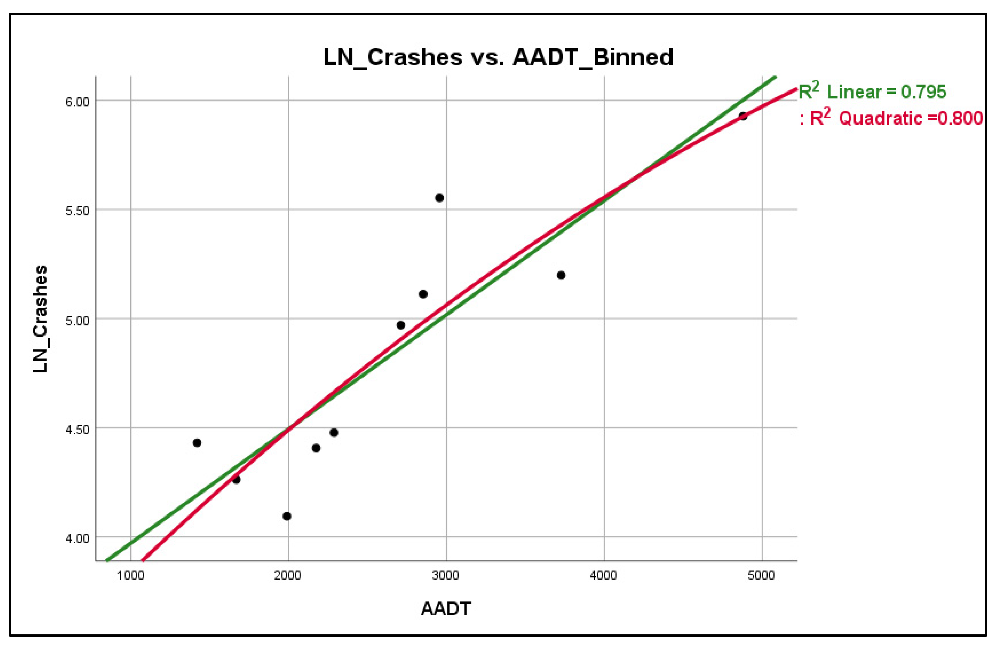
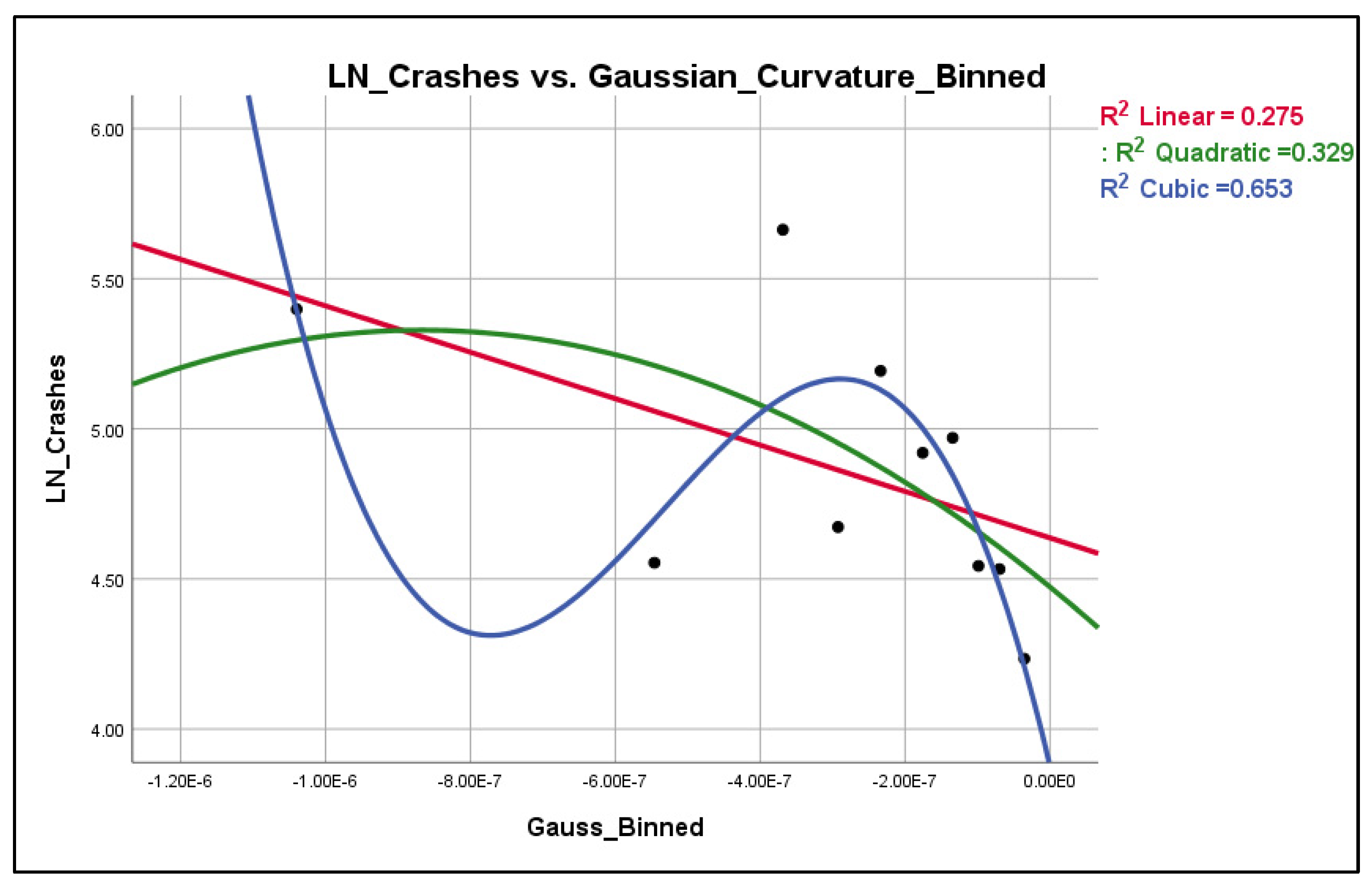
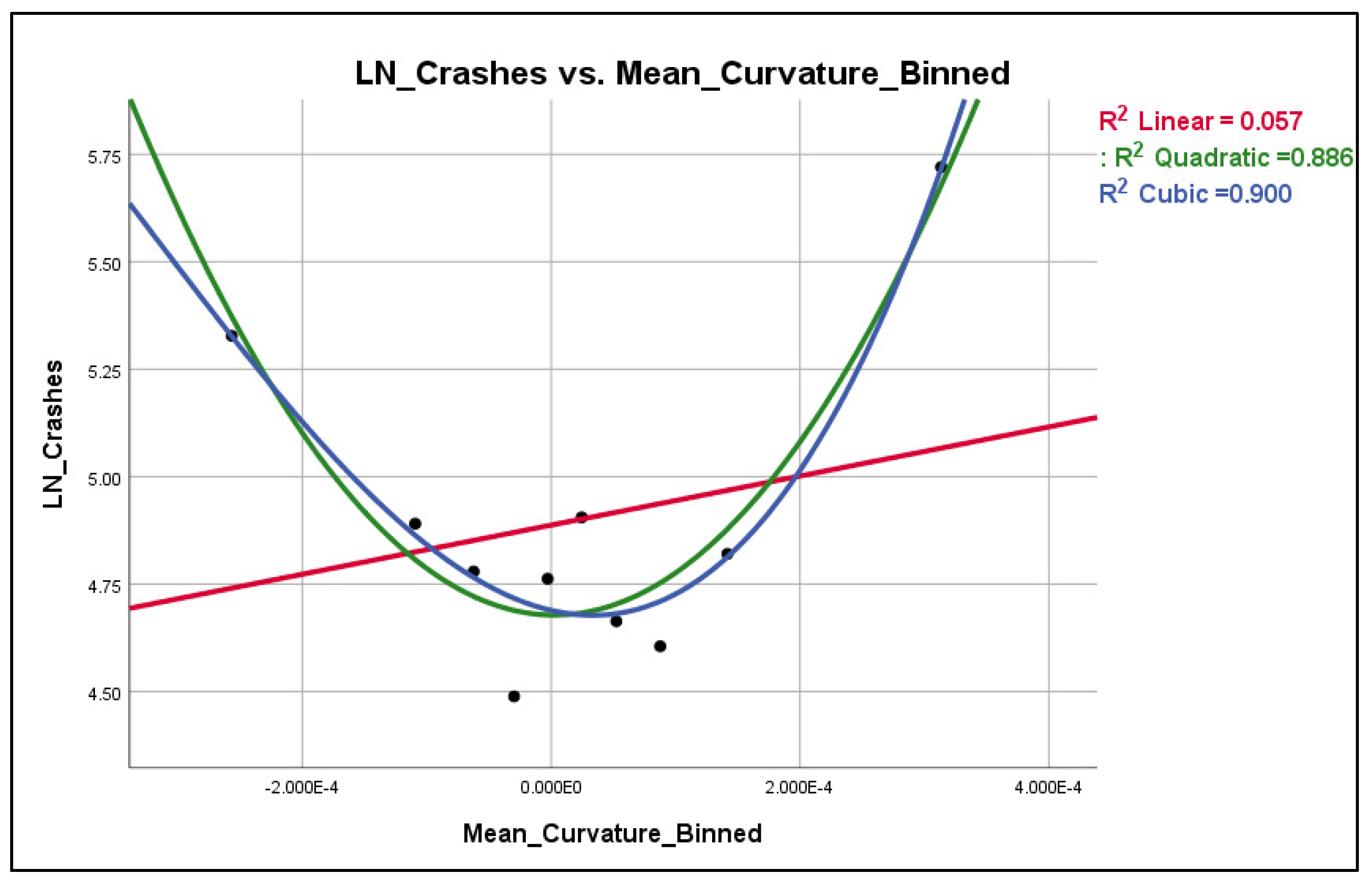
The typical visualization process in order to identify the optimal transformation of each explanatory variables is via scatterplots. The scatterplots for the explanatory variables AADT, GC, and MC are shown in Figure 5, Figure 6 and Figure 7, respectively, for the 100 ft patch.

According to Figure 5, AADT seems to have a rather linear relationship with LN(crashes), whereas Gaussian curvature (Figure 6) seems to have a cubic relationship with LN(crashes), and mean curvature (Figure 7) has an essentially quadratic relationship with LN(crashes). However, these observations hold true only when the explanatory variables are plotted one by one against the dependent variable; in other words, there is no guarantee that the nature of these relationships will remain the same when all of the explanatory variables enter the model. However, this procedure has revealed that, especially for the mean and Gaussian curvature, there is some indication that their relationship may not be linear in nature with LN(crashes) and therefore quadratic and cubic transformations may be appropriate for testing.

For each patch, 38 variable combinations were tested until the analysis was finalized. The models considered each variable alone and in a variety of combinations in order to determine the most appropriate and meaningful combination. All of these combinations for each patch length are presented in Amiridis, K. 2019, Appendix G [18]. The process for determining whether a model was appropriate was based on an initial determination of whether all of the coefficients of the model were statistically significant and accounting for the Bonferroni correction. Then the statistically significant models were compared with the AIC criterion. It is noted that, as a rule of thumb, when two models are compared and their AIC difference is greater than 10, then this difference is “significant”, meaning that the model with the lowest AIC should be kept instead (Hardin and Hilbe 2012) [26]. Finally, the assumptions according to which the model is based, e.g., normality of deviance residual distribution, must also be satisfied.

A summary of the variables used in the best models for each patch length are summarized in

Table 4. Variables present in final best models for each patch length.

Patch Length	Explanatory Variables
	AADT	GC	MC	GC2	GC3	MC2	MC3	AADT × MC	GC × MC
1500	X	X	X	X	X
1000	X	X		X	X		X
400	X	X	X	X	X	X
200	X	X	X	X	X			X
100	X	X	X	X	X	X			X
50	X	X	X	X	X	X			X

. Table 4 shows which explanatory variables were statistically significant without listing their corresponding coefficient values, as these may contain more than ten 10 significant digits, thereby compromising the readability of Table 4; however, the full numerical values are available in Amiridis, K. 2019, Appendix G [18]. The final suggested models as shown in Table 4 indicate that the Gaussian curvature (GC) and mean curvature (MC) of 3D surfaces play a crucial role in crash prediction since they are statistically significant in all models in which the Bonferroni correction has also been accounted for. In fact, not only are the Gaussian and mean curvature statistically significant in all models, but their p-values are also less than 0.001 in all models. The insertion of these two differential geometry metrics is actually the new aspect that this research introduces to the literature. The use of these metrics can be considered promising because the Gaussian and mean curvatures are the cornerstones of the study of 3D mathematical surfaces as a whole in differential geometry. Moreover, the fact that transformed geometric metrics, e.g., GC³ and MC², and the two-way interaction term GC*MC are inserted into the model, in the 100 ft patch length model, emphasizes the complexity by which roadway geometry affects crash occurrence, a fact that cannot be revealed in such an explicit manner through conventional 2D geometric metrics. Finally, in terms of computational statistics stability, when a variable is entered into a model with a power, e.g., quadratic, it is beneficial if the “lower power terms” are also included in the model, e.g., linear, for computational reasons. Fortunately, as demonstrated in Table 4, this is the case for both the GC³ and MC² variables since the variables GC² and GC, as well as MC, are also included in the model with p-values < 0.001, meaning that even the Bonferroni correction is amply satisfied.

The criterion used in order to select the most appropriate patch length was based on the overall error prediction which is estimated as the difference between the observed and model-predicted number of crashes. A summary of the predictive ability of each patch length, i.e., the associated error percentage to each, is shown in

Table 5. Patch length comparison in terms of predictive ability.

Patch Length (ft)	Predicted Crashes	Error Percentage of Total Crashes Predicted	PRESS
1500	1295	−15.6%	81.94
1000	1342	−12.5%	51.63
400	1582	3.1%	47.40
200	1546	0.8%	20.90
100	1532	−0.1%	15.93
50	1532	−0.1%	15.76

; it is noted that 1534 crashes occurred during the 2004–2017 period. Although it may be considered adequate on a practical basis to conclude that the 100 ft patch is the most pertinent patch length for the analysis, an additional statistical metric will also be considered to further validate this assertion, for the comparison among the different patch lengths. The additional statistical measurement used is the Predicted Error Sum of Squares or the so-called PRESS (Caroni and Oikonomou 2017) [27]. PRESS is used in order to compare regression models in terms of their ability to predict new values; the model preferred is the one with the smallest value of PRESS (Table 5).

The selected patch length for the final model corresponds to a length of 100 ft because it was observed that this patch length provides the best modeling ability. Even though a smaller patch length leads to an increase in the predictive power of the model, this was true up to a “cut-off” patch length, which in this case was estimated to be 50 ft. In this case, “cut-off” indicates that after a certain point the overall error is not practically improved with reduction of the patch length.

The results of the model corresponding to the 50 ft patch were identical to the ones derived from the 100 ft patch (Table 5). Moreover, a 100 ft patch may be considered more appropriate for transportation-related applications because vehicles that have a length over 50 ft such as combination trucks, recreational cars, and buses can be analyzed in a more reliable manner by incorporating a larger surrounding roadway geometry. Therefore, for transportation-related consistency and the practical effect of overall error reduction, as well as computational speed purposes, it was decided to utilize the 100 ft patch for the crash modeling process.

The final model corresponding to the 100 ft patch length is summarized in

Table 6. Coefficient values of final model (E35) for patch length = 100 ft.

Variable	Coefficient	p-Value
(Intercept)	−4.2701	0.000
AADT	0.00037	0.000
GC	−797,670.9567	0.000
GC2	−62,371,846,845.508	0.000
GC3	−101,722,389,759,530.720	0.000
MC	347.8188	0.000
MC2	209,377.3293	0.000
GC*MC	166,612,202.0693	0.000

, whereas the regression model is presented in Equation (1). The AIC for the models considered ranged from 11,183 to 11,803. The final model that was kept was indeed the one with the lowest AIC of 11,183 while the second-best model had an AIC of 11,232. It is noted that all of the explanatory variables of the final model have a p-value < 0.001, a fact that essentially demonstrates the proof-of-concept of this research: 3D geometric roadway metrics can successfully function as explanatory variables in crash predictive models.

$$LN\left(Crashes\right)=b0+b1 ·AADT+b2·GC+b3·{GC}^2+b4·{GC}^3+b5·MC+b6·{MC}^2+b7·(GC\ast MC)$$

(1)

As noted above, the presence of the Gaussian curvature and mean curvature of 3D surfaces supports the significance of these variables as crash predictors and their potential interaction with other variables—interactions that can by no means be captured in the 2D analysis.

At this point, the “Integrated Model” in which all years and roadways are included has been finalized and presented in Equation (1) above. The IM essentially functions as a proof-of-concept for the inclusion of the 3D metrics in crash prediction models and can, at least theoretically, be used for crash prediction purposes in other roadways. This model may be particularly useful when the purpose of an analysis is not the prediction of crashes in absolute numbers, but the comparison of alternatives, e.g., different alignments, in terms of estimating which alternative reduces crash frequency. In addition, it is suggested that the specific coefficient values (Table 6) be used for crash prediction purposes only when no historical crash data are available; if crash data are available for a specific roadway segment they should be certainly used in order to incorporate the “special crash pattern” in the adjusted model to be discussed in the next section. Finally, when several years of crash data are available, it is advised that, for crash prediction purposes, the years enter the model as dummy variables. The latter is suggested in order to account for seasonal and time effects. This is further discussed in the next section in which the predictive power of the model is evaluated.

The magnitude of regression coefficients reported in Table 6 should be interpreted in the context of variable scaling and transformation. Several explanatory variables, including curvature-based indicators, are derived from squared or higher-order geometric terms and are characterized by small numerical ranges. When such variables are included in a log-link negative binomial regression framework, relatively large coefficient values may result without implying unreasonable effects or numerical instability. Accordingly, coefficient interpretation in this study focuses on statistical significance, direction of effect, and contribution to model fit, rather than absolute magnitude. All coefficients were verified and found to be consistent with the underlying data and model specification.

3.2.2. Model Structure and Predictive Ability Evaluation

The ultimate objective of this research is the determination of the predictive ability of the proposed model based on 3D metrics on safety predictions. The comparison is based on the crash predictions as estimated from the model and the IHSDM. The IHSDM predicts crashes per year for a given roadway through the Empirical Bayes model. To account for the differences that arise throughout the years such as the number of crashes and AADT, IHSDM needs to develop a separate prediction for each year and this approach was considered and applied in the suggested model to obtain an accurate and fair comparison. It is therefore important to consider this in the model developed here and determine how to best approach it. There are two options for incorporating the “year effect” in this analysis: (1) use a separate model for each year developing predictions one year at a time; (2) insert dummy variables for years to account for the different AADT of each year. The following presents this analysis and the determination of which approach is more appropriate. It should also be noted that there is no concern whether the dummy variables are statistically significant or not at this point; their purpose is to simply increase the predictive ability of the model by accounting for the yearly variation of AADT and random effects in general.

The evaluation will be accomplished by creating training data, i.e., assuming that a certain year is not included in the dataset, running the analysis, and then predicting the crashes of that year and reporting the residuals. For example, the way in which the predictive power of the model will be evaluated for the year 2017 is as follows. Suppose that crash data are available for the years 2004–2016 and that the intention is to predict the crashes for the year 2017. The predictive model will include the explanatory variables of the IM, i.e., AADT, GC, GC², GC³, MC, MC², and GC*MC. Higher-order curvature terms are included as statistical representations of nonlinear geometric effects and are not intended to imply direct physical design variables. For the use of the dummy variable approach, in addition to the explanatory variables, a number of dummy variables equal to the number of years of crashes minus 1 is used. In this case, for the 13 years of available data (2004–2016 period), 12 (=13-1) dummy variables will be used. The crash predictions for the year 2017 will be calculated in the following form (Equation (2))

$$LN\left(13\ast Crashes\right)=b0+b1 ·AADT+b2·GC+b3·{GC}^2+b4·{GC}^3+b5·MC+b6·{MC}^2+b7·\left(GC\ast MC\right)+d1 ·D_{2004}+\cdots +d12 ·D_{2015}$$

(2)

or finally:

$$LN\left(Crashes\right)=b0+b1 ·AADT+b2·GC+b3·{GC}^2+b4·{GC}^3+b5·MC+b6·{MC}^2+b7·\left(GC\ast MC\right) + d1 ·D_{2004}+\cdots +d12 ·D_{2015}-LN\left(13\right)$$

(3)

The term “-LN(13)” is present in Equation (3) in order to convert the prediction model on a per-year basis since the model is based on 13 years of data. In statistical terminology, especially for GLM, this “-LN(13)” term is the so-called offset in the negative binomial regression (Hardin and Hilbe 2012) [26]. The crash predictions for any other year will be calculated with the same exact procedure and rationale. The model structure is evaluated using both approaches, with and without dummy variables, and then the predictions compared to the actual number of crashes. The approach that results in a prediction closer to the actual number of crashes would be the one used.

In

Table 7. Crash prediction estimates.

	KY420-1			KY420-2			KY152-1			KY152-2			KY152-3			US68-1			US68-2
Year	AC	W/O	W/	AC	W/O	W/	AC	W/O	W/	AC	W/O	W/	A	W/O	W/	AC	W/O	W/	AC	W/O	W/
2004	29	12	21	3	5	2	12	34	12	2	11	4	10	7	6	9	13	12	34	38	40
2005	15	12	15	0	4	2	8	34	9	4	11	3	8	7	5	6	12	9	30	38	30
2006	20	11	18	2	4	2	9	33	10	2	10	4	4	7	5	17	13	10	29	38	34
2007	21	11	14	3	4	2	3	31	8	1	10	3	3	7	4	6	13	8	30	38	27
2008	26	11	24	3	4	3	13	31	14	2	10	5	7	7	7	12	13	14	50	37	47
2009	33	11	23	3	4	3	8	31	13	6	10	5	5	7	7	17	13	14	38	37	45
2010	34	10	32	3	3	4	25	31	18	7	10	7	7	7	10	22	12	19	51	38	63
2011	30	10	35	0	3	4	21	30	20	8	9	7	8	7	10	26	12	20	72	38	68
2012	48	10	35	7	3	4	17	28	20	5	8	7	5	7	10	16	12	21	71	39	69
2013	28	11	29	2	3	3	10	26	16	10	8	6	4	7	8	13	12	17	68	39	56
2014	5	12	19	0	4	2	13	24	11	1	7	4	10	7	6	7	12	11	53	39	37
2015	12	13	23	3	5	3	17	23	13	5	6	5	7	7	7	18	12	13	42	37	45
2016	12	14	22	3	5	2	21	22	12	8	6	4	13	6	7	9	12	13	33	37	43
2017	12	14	15	4	5	2	7	22	9	5	6	3	6	6	5	12	12	9	24	36	30
Total	325	162	327	36	56	36	184	399	185	66	120	66	97	97	97	190	172	190	625	530	634
LEGEND
Notation											Description
AC											Actual Crashes
W/O											Predicted Crashes without Utilization of the Dummy Variables Approach
W/											Predicted Crashes with Utilization of the Dummy Variables Approach

, the crash prediction breakdown per year and roadway segment is presented in which there are three columns for each roadway segment: (1) actual crashes (AC); (2) predicted crashes without utilization of the dummy variables approach (W/O); (3) predicted crashes with utilization of the dummy variables approach (W/). In addition,

Table 8. Error comparison in crash prediction.

	KY420-1		KY420-2		KY152-1		KY152-2		KY152-3		US68-1		US68-2
	AC-W/O	AC-W/	AC-W/O	AC-W/	AC-W/O	AC-W/	AC-W/O	AC-W/	AC-W/O	AC-W/	AC-W/O	AC-W/	AC-W/O	AC-W/
2004	17	8	−2	1	−22	0	−9	−2	3	4	−4	−3	−4	−6
2005	3	0	−4	−2	−26	−1	−7	1	1	3	−6	−3	−8	0
2006	9	2	−2	0	−24	−1	−8	−2	−3	−1	4	7	−9	−5
2007	10	7	−1	1	−28	−5	−9	−2	−4	−1	−7	−2	−8	3
2008	15	2	−1	0	−18	−1	−8	−3	0	0	−1	−2	13	3
2009	22	10	−1	0	−23	−5	−4	1	−2	−2	4	3	1	−7
2010	24	2	0	−1	−6	7	−3	0	0	−3	10	3	13	−12
2011	20	−5	−3	−4	−9	1	−1	1	1	−2	14	6	34	4
2012	38	13	4	3	−11	−3	−3	−2	−2	−5	4	−5	32	2
2013	17	−1	−1	−1	−16	−6	2	4	−3	−4	1	−4	29	12
2014	−7	−14	−4	−2	−11	2	−6	−3	3	4	−5	−4	14	16
2015	−1	−11	−2	0	−6	4	−1	0	0	0	6	5	5	−3
2016	−2	−10	−2	1	−1	9	2	4	7	6	−3	−4	−4	−10
2017	−2	−3	−1	2	−15	−2	−1	2	0	1	0	3	−12	−6
Total	163	−2	−20	0	−215	−1	−54	0	0	0	18	0	95	−9
CI	161		20		214		54		0		18		86
LEGEND
Notation							Description
AC							Actual Crashes
W/O							Predicted Crashes without Utilization of the Dummy Variables Approach
W/							Predicted Crashes with Utilization of the Dummy Variables Approach
CI							Crash Prediction Improvement per Roadway Segment with the Dummy Variables Approach

presents the errors/residuals corresponding to the models with and without the dummy variable approach, as well as the corresponding crash improvement (CI) that has been achieved with the dummy variable approach.

The summary row in Table 8 denotes that the inclusion of dummy variables results in predictions that are closer to the actual number of crashes than those excluding them. Moreover, the insertion of dummy variables is preferred, in general, over the creation of separate models for each year because it is statistically more appropriate: the Bonferroni correction can be applied in a much more robust manner, since the familywise error is explicitly defined, and small sample size issues, which are in general present in crash datasets, are alleviated with the dummy variable approach.

Therefore, at this point it is decided to utilize the dummy variable approach in order to compare the crash predictions of the suggested model with those derived from the IHSDM. The comparison follows in the next section.

The next step involves evaluation of the assumptions of the model developed, since every regression model is based on some statistical, mostly distribution-related, assumptions. This applies in this case as well, and therefore these assumptions must be checked in order to validate the reliability of the model. In practical/applied terms, failure in assessing these assumptions would mean that the coefficients of the model are not reliable, i.e., the coefficients are inflated or deflated compared to the true parameters. Moreover, the defined confidence levels of the coefficients may not hold true, a fact that means that the exported p-values from the models may be highly distorted, which, in turn, means that although the model may be considered statistically significant based on the explanatory variables’ p-values, it may in fact not be statistically significant since the results may be only artificially in favor of rejecting the null hypotheses.

Many techniques have been suggested for the assumption assessment of regression models, but especially in the case of GLMs this matter remains an open research problem. Therefore, for the scope of this research, the basic assumption assessment techniques for which there is a general agreement in terms of their effectiveness and pertinence from the scientific community will be checked. More specifically, the assumption assessment was based on two elements: (1) residual analysis, and (2) influential points identification. Both residential analysis and influential points identification, via the Cook’s distance concept, are explicitly described in Amiridis, K. (2019) [18]. It is noted that the assumption assessment of the final regression model which corresponds to the 100 ft patch was conducted with success.

3.3. Comparison to Current Guidelines

This section evaluates the predictive ability of the suggested model with the current safety prediction methodology as utilized in the IHSDM. As described in the Methodology Section, crash predictions are derived through SPFs, which are the building blocks of the HSM. The equations of the HSM have been incorporated into the IHSDM which makes the calculations automatic. Moreover, the IHSDM can account for historical crash data and essentially adjust the crash prediction results through the Empirical Bayes model. Therefore, the results of the suggested model will be compared to those that would be obtained through the IHSDM. The comparison results are based on the prediction models obtained by applying a 100 ft patch for the 3D roadway surface.

Table 9. Crash prediction estimate comparison.

	KY420-1			KY420-2			KY152-1			KY152-2			KY152-3			US68-1			US68-2
	AC	IH	SU	AC	IH	SU	AC	IH	SU	AC	IH	SU	AC	IH	SU	AC	IH	SU	AC	IH	SU
2004	29	25	21	3	8	2	12	21	12	2	7	4	10	11	6	9	18	12	34	49	40
2005	15	25	15	0	8	2	8	21	9	4	8	3	8	11	5	6	18	9	30	49	30
2006	20	25	18	2	8	2	9	22	10	2	8	4	4	12	5	17	18	10	29	51	34
2007	21	25	14	3	8	2	3	22	8	1	8	3	3	12	4	6	19	8	30	51	27
2008	26	25	24	3	8	3	13	21	14	2	8	5	7	11	7	12	19	14	50	49	47
2009	33	24	23	3	8	3	8	21	13	6	8	5	5	11	7	17	18	14	38	50	45
2010	34	24	32	3	9	4	25	21	18	7	7	7	7	11	10	22	18	19	51	49	63
2011	30	24	35	0	9	4	21	21	20	8	8	7	8	11	10	26	18	20	72	48	68
2012	48	23	35	7	8	4	17	21	20	5	8	7	5	11	10	16	18	21	71	47	69
2013	28	26	29	2	8	3	10	21	16	10	8	6	4	11	8	13	19	17	68	47	56
2014	5	27	19	0	9	2	13	21	11	1	8	4	10	11	6	7	19	11	53	49	37
2015	12	26	23	3	8	3	17	22	13	5	8	5	7	11	7	18	18	13	42	50	45
2016	12	26	22	3	8	2	21	21	12	8	7	4	13	11	7	9	19	13	33	51	43
2017	12	25	15	4	8	2	7	21	9	5	8	3	6	11	5	12	18	9	24	49	30
Total	325	351	327	36	116	36	184	296	185	66	106	66	97	156	97	190	257	190	625	691	634
LEGEND
Notation											Description
AC											Actual Crashes
IH											Predicted Crashes Produced by the IHSDM Software
SU											Predicted Crashes Produced by the Suggested Model

presents the crash prediction breakdown per year and roadway segment. There are three columns for each roadway segment: (1) actual crashes (AC); (2) predicted crashes produced by the IHSDM software 17.0 (IH); (3) predicted crashes produced by the suggested model (SU). In addition,

Table 10. Error comparison in crashes.

CI*	24	80	111	40	59	67	57
CI PM*	17	91	13	18	17	12	5
CI PY*	2	6	8	3	4	5	4
CI PM PY*	1.2	6.5	0.9	1.3	1.2	0.8	0.4

CI*: Crash improvement per roadway segment with the suggested model compared to the IHSDM. CI PM*: Crash improvement per roadway segment per mile with the suggested model compared to the IHSDM. CI PY*: Crash improvement per roadway segment per year with the suggested model compared to the IHSDM. CI PM PY*: Crash improvement per roadway segment per mile per year with the suggested model compared to the IHSDM.

presents the error/residual comparison between the suggested model and the IHSDM, as well as the corresponding crash prediction improvement (CI) that has been achieved with the suggested model. The crash prediction differences will also be presented per mile as well, since this is another unit that the IHSDM utilizes.

Table 9 show that the crash prediction results produced by the suggested model are more comparable to the actual crashes than those obtained from the IHSDM, which is the current crash prediction practice. This could be seen as an indication of the beneficial effects that 3D geometric metrics can offer to highway safety. Another fact that makes this research promising is that the comparison is conducted in a quantifiable manner. However, although the improvement in crash prediction is an important issue on its own, this improvement should be demonstrated not only in crash units, but also in monetary value. Although one may argue, on a philosophical level, that human life is priceless, this approach does not convey the whole truth as implemented in practice. It is true that even fatalities, injuries, and property damage are incorporated into an optimization scheme in order to reach decisions during the planning/budgeting phase of a project that would eventually have an optimal effect on society as a whole. For example, although it may be observed that the crash occurrence on a particular roadway is problematic, a cost–benefit analysis is typically conducted to determine how to best allocate limited resources to increase their effectiveness. Such improvements are then compared to other competing projects and needs, and decisions are reached based on optimizing the available funds for the greater good of the system.

Varying crash predictions can lead to vastly different decisions because they are essentially tightly linked to the cost estimation of a project, new or existing, that is considered to be modified. It is therefore imperative that predictions are accurate to avoid assigning incorrect priorities while addressing needs. Although crash costs are just a portion of the total project cost, there are substantial in both economic and societal terms. Crash overprediction may yield a project too expensive, leading to its rejection, whereas crash underprediction will lead to under design problematic issues and inflated crash occurrence.

Considering the potential impact of the overestimation of the IHSDM as compared to the suggested model, one can surmise that when cost–benefit estimates are required for projects these could be grossly miscalculated and thus potentially result in addressing the wrong projects. More accurate cost estimation procedures can greatly benefit both public agencies and private companies during the bidding phase of a highway engineering project because their estimations will be in line with reality in a more reliable manner. Moreover, tax payers can feel more confident that their contribution is invested in a better way and in the long run public agencies could potentially design and construct additional infrastructure projects, such as schools and parks, with the same initial budget.

Thus, at this point, the intended proof-of-concept of the research, i.e., 3D differential geometry metrics have a crash prediction value, has been established and the final model has been compared to the current practices through the use of the IHSDM. The latter comparison verified that the results derived from the suggested model, containing 3D explanatory variables derived from differential geometry, are closer to the actual/observed crashes, compared to the SPFs of the HSM.

An advantage of the proposed model is that it only requires XYZ data of the roadway instead of the detailed geometric data input of the IHSDM which requires as input the horizontal and vertical alignment information. Therefore, the proposed model is more flexible than the IHSDM. In addition, if the horizontal and vertical alignment plans are not available, then it is difficult, if not impossible, to utilize the IHSDM, since these are essential inputs for the calculation process. The data entry in the IHSDM is also a tedious process and demands manual entry. The proposed model takes advantage of the automated conversion from 3D XYZ data to horizontal and vertical alignment via the FM-17 software offered by the National Technical University of Athens’ Department of Civil Engineering. The FM-17 offers some semi-automatic tools that assist in the 3D to 2D conversion, but the procedure remains subjective and demands manual correction at the end of the process.

4. Conclusions and Future Research

This study examined the applicability of surface-based three-dimensional (3D) geometric indicators in traffic crash frequency analysis. The objective was to evaluate whether curvature measures derived from a continuous 3D roadway surface can provide meaningful explanatory information beyond that offered by conventional two-dimensional alignment indicators.

A 3D roadway modeling framework was implemented using B-spline surface representations, allowing Gaussian curvature and mean curvature to be computed as patch-level geometric descriptors. Crashes were spatially allocated to surface patches and analyzed using negative binomial regression models with traffic exposure accounted for through annual average daily traffic. The results demonstrate that surface-based curvature indicators are statistically significant predictors of crash frequency and are capable of capturing combined geometric effects that are not explicitly represented by traditional alignment measures.

The key contribution of this work lies in demonstrating, through a proof-of-concept analysis, that roadway geometry can be represented and evaluated as an integrated 3D surface for safety analysis purposes. Rather than replacing established design indicators or prediction models, the proposed approach provides a complementary framework that enables the incorporation of geometric interactions within a unified analytical structure.

Future research may extend this framework by incorporating additional surface-based indicators, larger and more diverse datasets, and alternative modeling techniques. The proposed methodology offers a foundation for further investigation into integrated 3D representations of roadway geometry in highway safety analysis.

The dataset used in this study spans a 14-year period (2004–2017), during which changes in vehicle technology, traffic enforcement, and safety policies may have occurred. While such factors can influence overall crash rates, the analysis assumes that roadway geometric characteristics remained unchanged throughout the study period. This assumption allows the investigation to isolate the relationship between roadway geometry and crash occurrence, which is the primary focus of this research. Temporal variations related to policy or technology changes are therefore treated as background effects rather than explicit explanatory variables.

In addition, the analysis is limited to selected rural roadway segments with consistent geometric characteristics. As a result, the findings should not be interpreted as universally generalizable across all roadway types or geographic regions. Instead, the results are intended to demonstrate a proof-of-concept for applying surface-based three-dimensional geometric indicators in crash analysis. Future research should extend this framework to additional roadway classes, geographic regions, and time periods to further evaluate robustness and generalizability.

Future Research Recommendations

Many recommendations for future research can be made since the incorporation of 3D metric in the highway design process is a rather unexplored field. Some suggestions are presented in this section.

A major concern of this research was the determination of the patch length, which the statistical analysis was based upon. A future step would be to create a mesh on the roadway surface whose patches would not necessarily have equal lengths, but would alter depending on the special geometric properties of the surface each time. This mesh would look like the meshes that are utilized in the Finite Element Method (FEM). The meshing criteria would be related to the Gaussian and mean curvature values of the 3D B-spline roadway surface. In practical terms, this means that the mesh would be denser in surface areas, i.e., on the roadway surface, that have larger values of Gaussian and mean curvatures and sparser in surface areas that are more “flat”. It is anticipated that this may increase the predictive ability of the model as well as the computational speed of the procedure. Moreover, it may be easier to identify problematic roadway segments in terms of highway safety due to the more accurate construction of the underlying mesh, which would be purely based on the differential geometry properties of the roadway surface and implemented with computational geometry techniques.

In this research, the shoulder width is not included as an explanatory variable because all roadway segments have the same shoulder width and therefore no differentiation is possible in the statistical analysis. The shoulder is not modeled as part of the 3D B-spline surface because the driver does not, at least typically, travel on the shoulder. However, the intension is to include additional metrics directly related to highway design such as shoulder widths and lane widths in regression models in the future. This task can be accomplished with the inclusion of dummy variables: for example, dummy variables pertaining to shoulder widths of 4 ft, 6 ft, 8 ft, and 10 ft, as well as dummy variables corresponding to lane widths of 10 ft, 11 ft, and 12 ft. However, in order for this to be feasible, sample roadway segments containing all of these combinations of shoulder and lane widths, as well any other highway design characteristic desired, should be retrieved and included in the statistical analysis. Nonetheless, at this point CMFs can be incorporated into the suggested 3D models, creating hybrid 3D SPFs. For example, since this research was conducted for 11 ft lane width roadways, CMFs can be utilized in order to adjust the crash predictions for different lane widths accordingly; in other words, at this point, 11 ft lane widths function as the baseline conditions, as defined in the HSM terminology, of the analysis. In general, more explanatory variables of both highway design, e.g., roadside characteristics, and 3D geometry oriented, e.g., length of geodesic curves and 3D stopping sight distance, should enter the model. Finally, the rationale, results, and findings of this research can be integrated into the current highway design practices, e.g., IHSDM software, in order to enhance them, by adding/incorporating the 3D metrics used here into existing SPFs.

The severity type of the crash should be incorporated into the regression models. In this case, small-sample-size-related issues will surely arise, but research should move towards this direction even if it requires waiting some years in order for more crash data to be accumulated. A more detailed breakdown in terms of crash severity type would eventually allow for a more detailed crash cost estimation since, as one would expect, different crash costs are associated with different crash types (FHWA, n.d) [28]. Moreover, the present study focuses on rural two-lane highways to control confounding effects; extension to urban and mountainous networks is left for future work.

The ultimate objective of this research would be to develop user-friendly and interactive software/tools that would be able to be incorporated into highway design software programs, e.g., Autocad Civil 3D and Microstation, in order to assist in the design process. This tool would be particularly useful for the evaluation and comparison of alternative/competing highway geometric alignments. In addition, this tool would be able to express the evaluation of alternative alignments not only in terms of an increase/decrease in crashes, but also in terms of the associated crash cost. Finally, this system could be integrated into the GPS screen of vehicles in order to warn drivers when driving on roadway segments in which the crash occurrence probability calls for proportionally more attention.