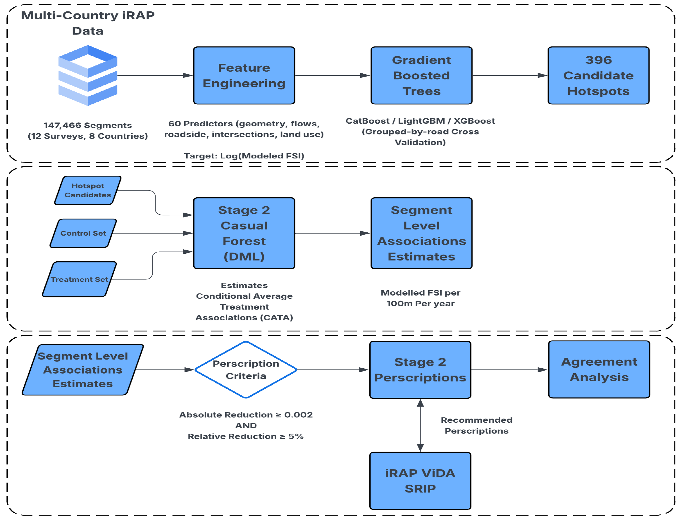
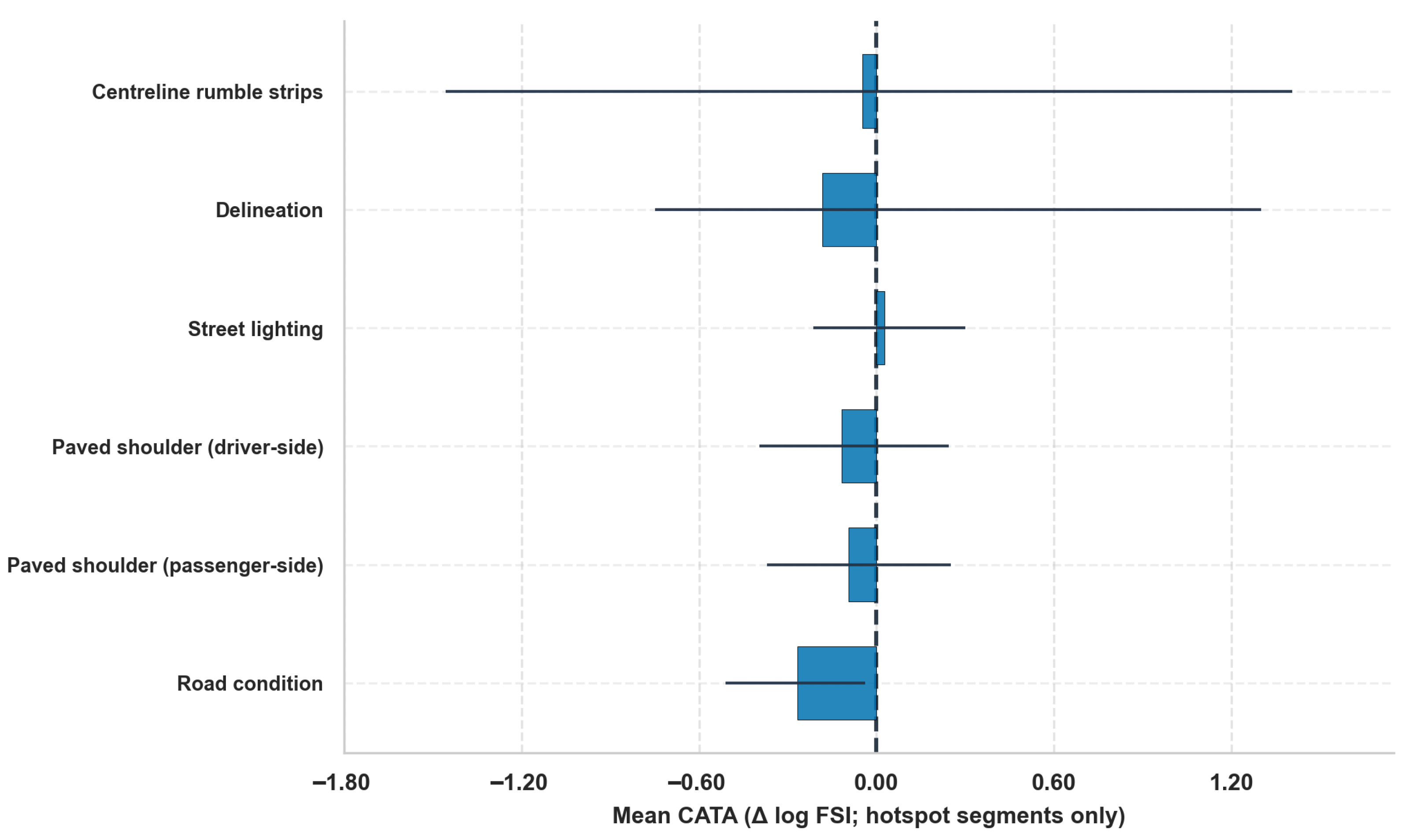
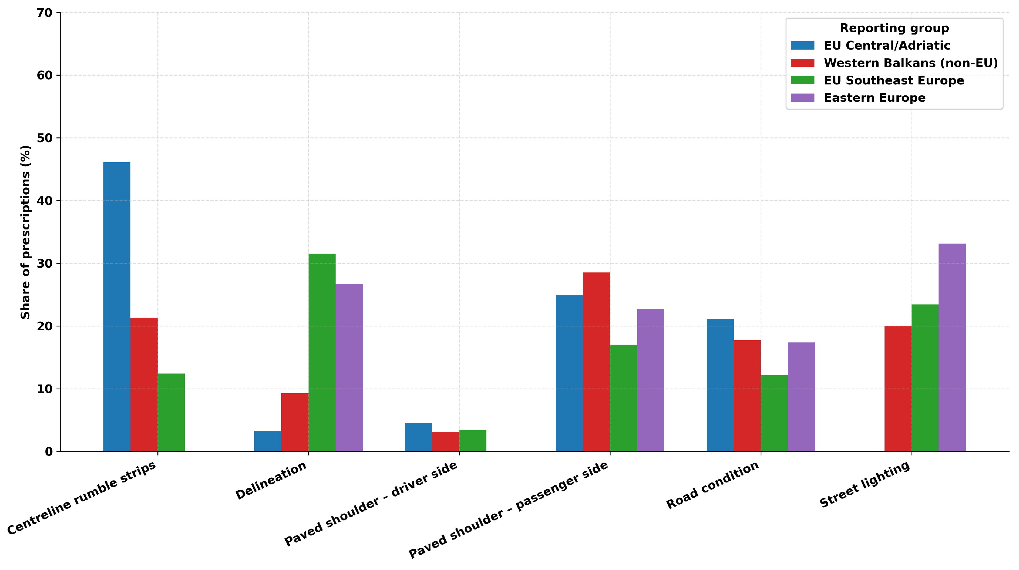
We describe Stage 1 surrogate modelling and SHAP-based interpretation, hotspot selection and diagnostics, Stage 2 treatment-association estimation using double machine learning with causal forests, and the comparison with SRIP recommendations.
4.1. Stage 1 Predictive Modelling and Explanation
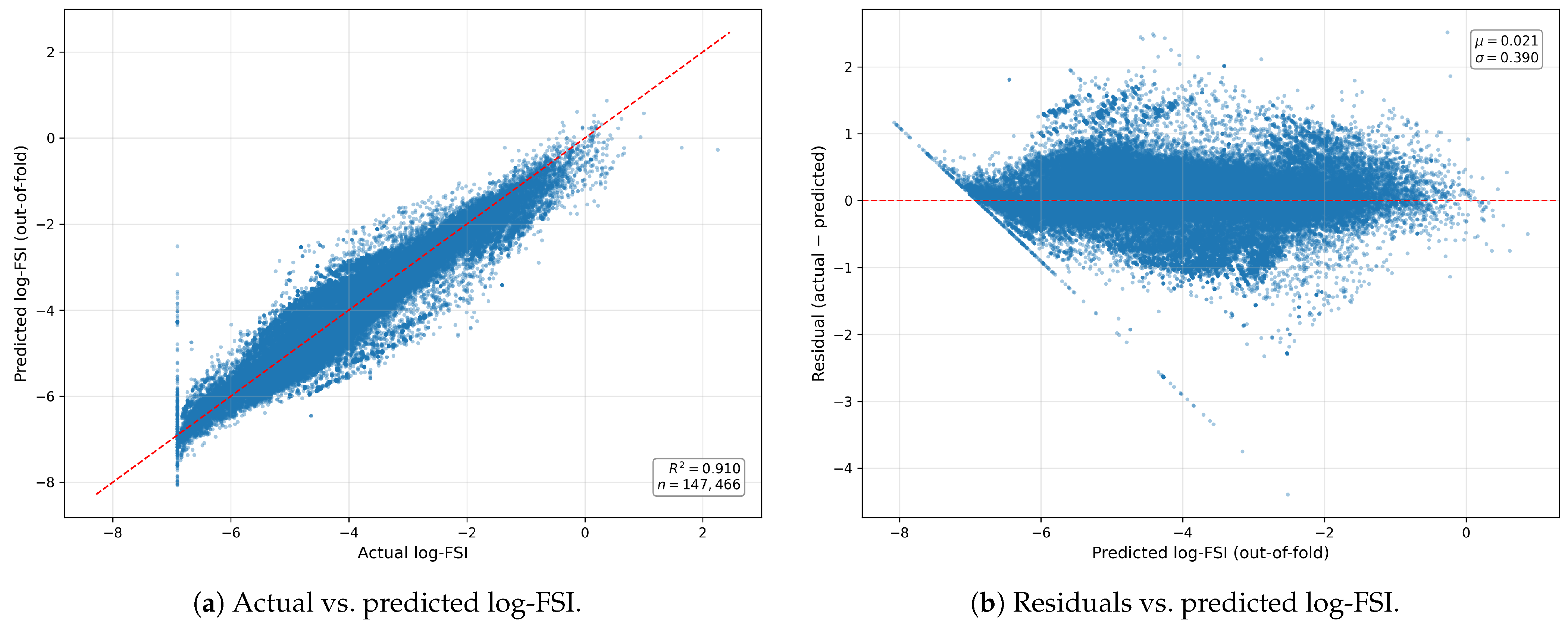
The first stage of the framework uses tree-based ensemble models to approximate the iRAP-modelled FSI on a log-transformed scale and to identify high-risk segments for further analysis. Following the data preparation described in
Section 3, the target variable is
for segment
n, and the predictor set consists of the Stage 1 predictors in
Table 2, including the Dataset ID in the main specification used for hotspot selection and excluding any direct outputs of the iRAP risk engine.
We considered three gradient-boosted tree families that are widely used in crash prediction and injury severity modelling [
16,
17,
32]: CatBoost [
51], LightGBM [
52], and XGBoost [
53]. All models operate on the same training matrix and are evaluated using an identical cross-validation scheme. To avoid spatial leakage and to reflect typical use cases where whole roads are assessed, we use grouped cross-validation by road. All segments belonging to a given named road are assigned to the same fold, and in each iteration, one group of roads is held out as a test set while the models are trained on the remaining roads. This configuration ensures that out-of-fold predictions for each segment are based only on models that have not seen any other segment from the same road.
The hyperparameters for each model family are tuned with a Bayesian Tree-structured Parzen Estimator (TPE) sampler [
54], using the mean grouped-by-road cross-validated
as the objective. Each model runs up to 150 trials under the same cross-validation scheme, and the best configuration is then used to generate out-of-fold predictions for all segments. For CatBoost, the search also includes the number of trees and bagging-related parameters, whereas for LightGBM and XGBoost, it explores leaf-wise growth depth and minimum child weight. The selected hyperparameters are listed in
Table 3.
The best configuration for each model is then retrained in a cross-validation manner to obtain out-of-fold predictions for all segments. These predictions, together with the true log-FSI values and fold identifiers, are stored in a master file that underpins all diagnostics, hotspot selection, and later analyses. Detailed performance metrics and sensitivity checks are reported in
Section 5.1.
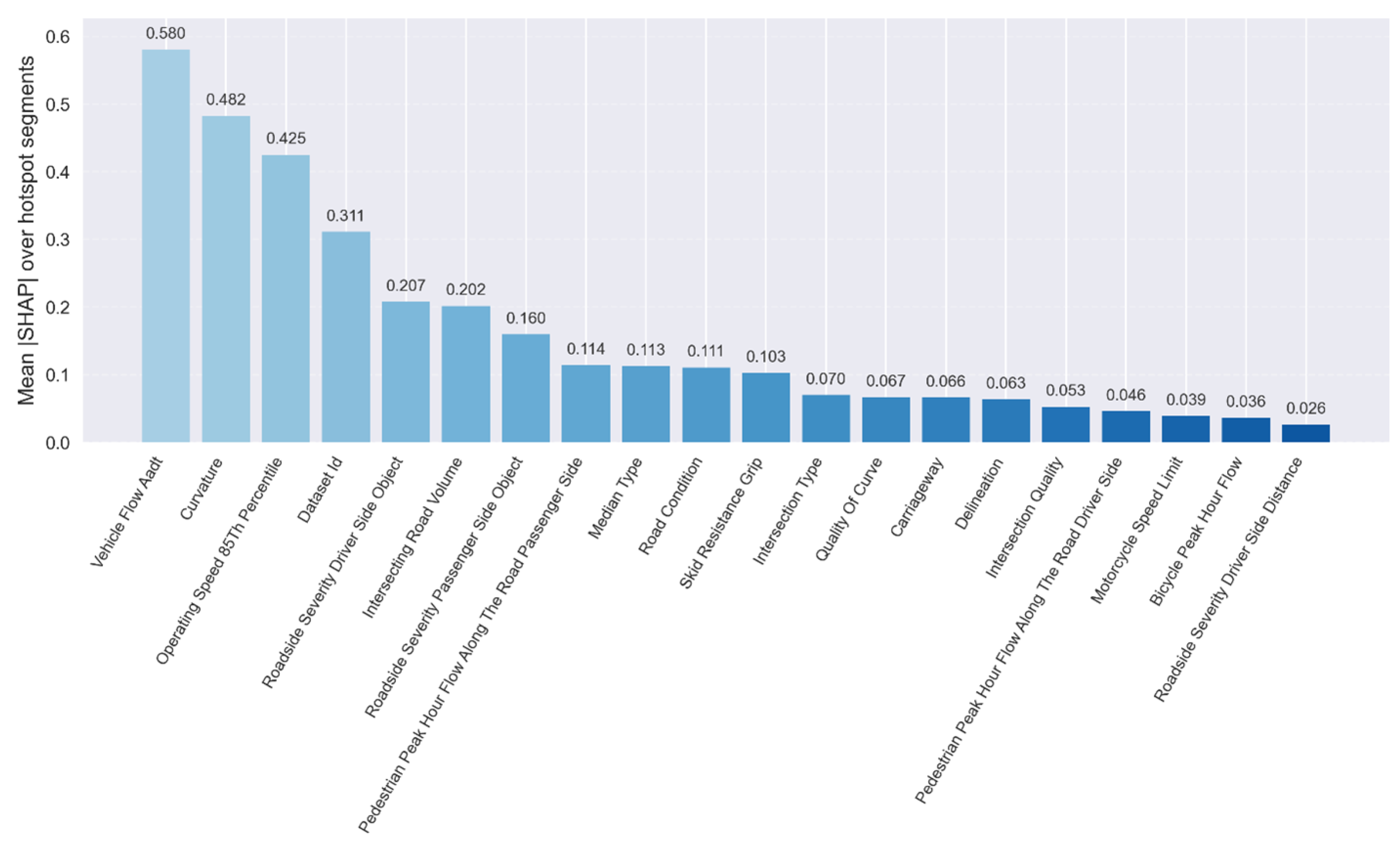
Model interpretation in Stage 1 relies on SHAP values [
55] computed for the selected CatBoost model on the log-FSI target [
20,
21]. SHAP provides a local decomposition of the prediction at each segment into feature contributions. To align explanations with the later treatment-association analysis, we compute SHAP values only for the predicted hotspots using out-of-fold models. For each fold, we rank segments within each road by out-of-fold predicted risk, select the top three per road, and compute SHAP values for those segments using the corresponding fold model. We then aggregate the absolute SHAP values across the hotspots to obtain a global feature ranking. These SHAP analyses describe how the predictive model combines infrastructure attributes and flows in high-risk segments, but they are not interpreted as causal effects.
4.3. Stage 2 Treatments, Controls, and Identification Assumptions
Stage 2 estimates segment-level associations between actionable infrastructure treatments and the modelled FSI outcome network-wide using a double-machine-learning (DML) causal forest. We report hotspot-level summaries and prescriptions on the Stage 1 candidate hotspots (
Section 4.2). The treatment and control sets are defined in the project configuration and checked against hotspot data using simple summary tables of level distributions. Treatments were selected according to the following criteria: actionability, interpretability, and statistical support.
First, a candidate variable must correspond to an infrastructure change that can realistically be implemented as a retrofit on an existing road within the scope of typical safety projects rather than requiring large-scale reconstruction or major land use change. Second, the coding of the variable must have a small number of ordered levels or a binary form so that the contrast is interpretable for engineers. Variables with many unordered categories would require arbitrary collapse, which makes it difficult to map estimated associations to concrete design actions. Third, each level of the candidate treatment must have sufficient representation in the full eligible segment corpus (and also in the hotspot subset for reporting), so that the causal forest does not have to extrapolate into parts of the covariate space with little data. Only six variables satisfy all three criteria, and these form the treatment set in Stage 2. These are:
Centreline rumble strips, coded as a binary variable indicating presence versus absence, with the action being the installation or upgrade of strips on undivided roads.
Delineation, coded as a binary variable indicating adequate versus poor markings, with the action of repainting or improving markings and posts.
Street lighting, coded as a binary indicator of lighting presence, with the action being the installation or upgrade of fixed roadway lighting.
Paved shoulder—driver side, coded on a four-level ordinal scale from wide sealed shoulder to narrow, unpaved, or none, with the action being to pave and widen the poor shoulders.
Paved shoulder—passenger side, coded on the same four-level ordinal scale for the passenger side.
Road condition, coded on a three-level ordinal scale from good to fair to poor pavement, with the action of resurfacing or rehabilitation of poor segments.
Ordinal codes are defined such that lower values represent better conditions (shoulders: 4 worst → 1 best; road condition: 3 poor → 1 good), and Stage 2 targets one-level improvements.
Level-distribution checks confirm sufficient representation for all six variables in both the full corpus and the hotspot subset.
All Stage 2 models adjust for a pre-specified control set of 38 variables covering exposure, geometry, cross-section, roadside environment, pedestrian facilities, intersections, speed environment, and survey metadata. The Stage 1 models were trained on the candidate predictor set as shown in
Table 2. For hotspot selection, we use the Dataset-ID-included specification. Sensitivity checks re-estimate Stage 1 (i) without Dataset ID and (ii) under the reduced-information specification, excluding the supporting exposure/speed inputs listed in
Table 2. For Stage 2, we define six treatments and a separate set of 38 controls from the cleaned attribute pool, excluding 15 candidate variables after a validation sweep that checked actionability, coding quality, and statistical support. A full list of treatments and controls is provided in
Table 4 and
Table 5, respectively.
In contrast, some imbalanced but well-defined features are deliberately retained as control variables when they provide important roadway context. For example, shoulder rumble strips are an unbalanced binary code in this sample; nevertheless, their presence is typically characteristic of specific facility types (e.g., rural, higher-speed segments with run-off-road mitigation) and therefore serves as a marker of the broader design and operating environment. We retain this variable as a control to help adjust for systematic differences in road class and cross-section that co-vary with both treatment coding and the modelled outcome. In summary, Stage 2 uses a confounder-rich but quality-screened control set. The feature-classification logic is documented in the code repository.
The modelling strategy follows common assumptions used in causal machine learning, applied here to a deterministic model output. Conditional on the control set, we assume that the treatment codes are not systematically correlated with omitted coded context that also shifts the ViDA modelled outcome and that there is sufficient overlap in treatment prevalence across covariate profiles to support comparisons. We assess overlap using prevalence summaries on the full corpus and on the hotspot subset (
Table A1).
In addition, we report treatment-prevalence summaries on the full corpus and on the hotspot subset, and compute treatment-level covariate-balance diagnostics (standardised mean differences for the retained controls). These summaries are used to flag comparisons that rely on weak support and are interpreted conservatively in
Section 6. In particular, they help identify contrasts with weaker empirical support, especially where rare treatment levels create limited overlap. Scripts for generating the full prevalence and covariate-balance tables are available in the code repository.
Including Dataset ID as a control helps absorb systematic survey-level shifts, including calibration and other contexts that are constant within a survey. Because the outcome is the ViDA modelled FSI (see
Section 1), the causal forest is used to reverse-engineer and audit the effective response surface of the risk model.
4.4. Causal Forest Estimation and Prescription Rule
Stage 2 uses a causal forest [
42,
56,
57] within a double machine learning (DML) framework [
58,
59], to estimate segment-level conditional average treatment associations for each of the six treatments (
Table 4) on the modelled FSI outcome across the full eligible segment corpus. For a given treatment
T and outcome
Y (the log-transformed modelled FSI), we define a conditional surface contrast on the exported ViDA output:
where
X denotes the vector of control variables described above.
The outcome Y used in Stage 2 is the actual log-transformed ViDA export, not the Stage 1 prediction. Stage 1 outputs are used only for hotspot definition, hotspot ranking, and hotspot-level interpretation.
For ordinal treatments (paved shoulders and road condition), we estimate adjacent-step contrasts that match a one-level upgrade rule. Specifically, for each ordinal treatment we consider contrasts of the form toward a better code (e.g., shoulders , , ; road condition , ). We compute these contrasts directly rather than treating the ordinal code as a continuous scalar slope. We denote the resulting segment-level estimates as conditional average treatment associations (CATA). We use CATA rather than CATE because the outcome is the exported ViDA modelled FSI and the quantity is interpreted as an association contrast on that modelled surface rather than as a causal effect on observed crashes. For each adjacent-step contrast, we restrict estimation to segments whose current code equals either t or and define a binary treatment indicator with for the better level () and for level t.
The causal forest is implemented within a double machine learning framework that follows recent work on heterogeneous treatment estimation in transport and related fields [
11,
22,
23,
24,
25]. For each treatment contrast, we estimate an outcome model
using a random forest regressor and a propensity model
using a random forest classifier, both with 500 trees, maximum depth 10, minimum leaf size 5, and the square root of the number of features as the splitting subset. Five-fold road-grouped cross-fitting is used, where all segments from the same named road are assigned to the same fold and folds are stratified by Dataset ID so that each fold preserves the survey composition of the full corpus. Orthogonalised outcome and treatment residuals are formed on held-out folds. For the binary adjacent-step treatment contrasts, the propensity score is the out-of-fold predicted probability returned by the random-forest classifier within this grouped cross-fitting procedure. Estimated propensities are trimmed to the interval
to stabilise inverse-probability weights in regions of weak overlap. The final-stage causal forest is trained on these residuals together with
X, using 1000 trees, maximum depth 8, minimum leaf size 50, and two Monte Carlo iterations. The forest splits on control variables to find regions where the residual association is approximately stable, producing a segment-level association estimate
.
Cross-fitting and regularisation inherent to causal forests (subsampling and minimum leaf sizes) mitigate overfitting in heterogeneous association estimation. This procedure is repeated separately for each of the six treatments, with the remaining five treatments and all other covariates used as controls. Therefore, each estimated association is conditional on the current pattern of the other five treatments, and the forest does not attempt to model the joint effect of treatment bundles. The result is a set of six vectors of segment-level associations , one for each treatment k, defined on the log-FSI scale. For reporting and decision making, these log-scale associations are converted back to the original FSI scale by applying the inverse of the log transformation at the segment-specific baseline risk. With , a segment-level log-scale association corresponds to an implied change on the natural scale of .
Road-level empirical Bayes shrinkage.Because roads vary widely in length (and therefore in the number of 100 m segments contributing to each road-level mean), raw segment-level CATA estimates can be noisy for short roads. We stabilise them with an empirical Bayes (James–Stein) shrinkage step. For each road
r with
valid segments, we compute a shrinkage weight
with
and pull the road-level mean toward the global mean:
where
is the raw road mean and
the global mean. Segment-level deviations within each road are scaled by the same weight:
. This attenuates estimates for roads with few segments while leaving well-supported roads largely unchanged.
The final step in Stage 2 is to convert the segment-level association estimates into a set of recommended prescriptions. For each hotspot
n and treatment
k, we use the estimated log-scale association
and the segment’s baseline FSI to compute an implied change in the modelled FSI per 100 m per year,
. We summarise this as an absolute reduction
and a relative reduction
where the
term is used only to avoid division by zero when
. A treatment
k is recommended for segment
n if and only if both thresholds are met:
These thresholds enforce a minimum practical impact in absolute terms and minimum proportional reduction relative to the segment baseline. The candidate upgrades are triggered only by the absolute and relative reduction thresholds in (
9) and (
10). Each output consists of a hotspot, a recommended treatment, and the associated estimated change in the modelled FSI.
Uncertainty reporting. Because hotspot retrieval is evaluated under road-grouped generalisation, we use a road-cluster bootstrap for the Stage 1 hotspot retrieval metrics and the Top-K sensitivity analysis. Stage 2 SRIP agreement metrics are reported descriptively in this version.
4.5. Comparison with iRAP ViDA Recommendations
The final part of the methods compares Stage 2 prescriptions with the countermeasures generated by the iRAP ViDA Safer Roads Investment Plan (SRIP) to quantify agreement and to analyse where the two systems diverge. All comparisons are restricted to the six treatment classes defined in
Section 4.3.
First, we construct a common representation of the treatments. The iRAP SRIP outputs contain a detailed list of the recommended countermeasures with project-specific labels. To make this comparison, we select SRIP countermeasures that can be mapped to the six treatment classes used in Stage 2. We use the full mapped SRIP export, i.e., the list of technically feasible countermeasures returned by ViDA before later benefit/cost shortlist filtering. This set still reflects SRIP’s built-in feasibility, compatibility, and hierarchy constraints (e.g., spacing rules and treatment hierarchies). By contrast, project-specific discount rates, economic values, and BCR thresholds affect later shortlist formation rather than the segment-level FSI engine itself.
Using a study-specific mapping table, each SRIP countermeasure is assigned to one of the six treatment classes defined in
Section 4.3. For example, various forms of line marking upgrade are mapped to delineation, and shoulder surfacing options are mapped to the appropriate paved shoulder treatment. SRIP recommendations that cannot be mapped cleanly to one of these six classes, such as major intersection reconstruction or access management measures, are excluded from the comparison, so that both systems are evaluated in the same treatment space.
Second, we identify an overlapping hotspot set. From the hotspot ledger and the iRAP SRIP outputs, we select 321 Stage 1 candidate hotspots where iRAP has SRIP coverage and at least one SRIP countermeasure can be mapped to our six treatment classes. For each hotspot and treatment, we form two binary indicators: one indicating whether Stage 2 recommends the treatment and another indicating whether SRIP recommends it. If multiple SRIP records map to the same treatment class on the same segment, we set the segment–class indicator to 1 if any record exists (i.e., deduplicate at the segment–treatment-class level). This yields a table with one row per segment and treatment combination, which we use for the classification-style agreement measures.
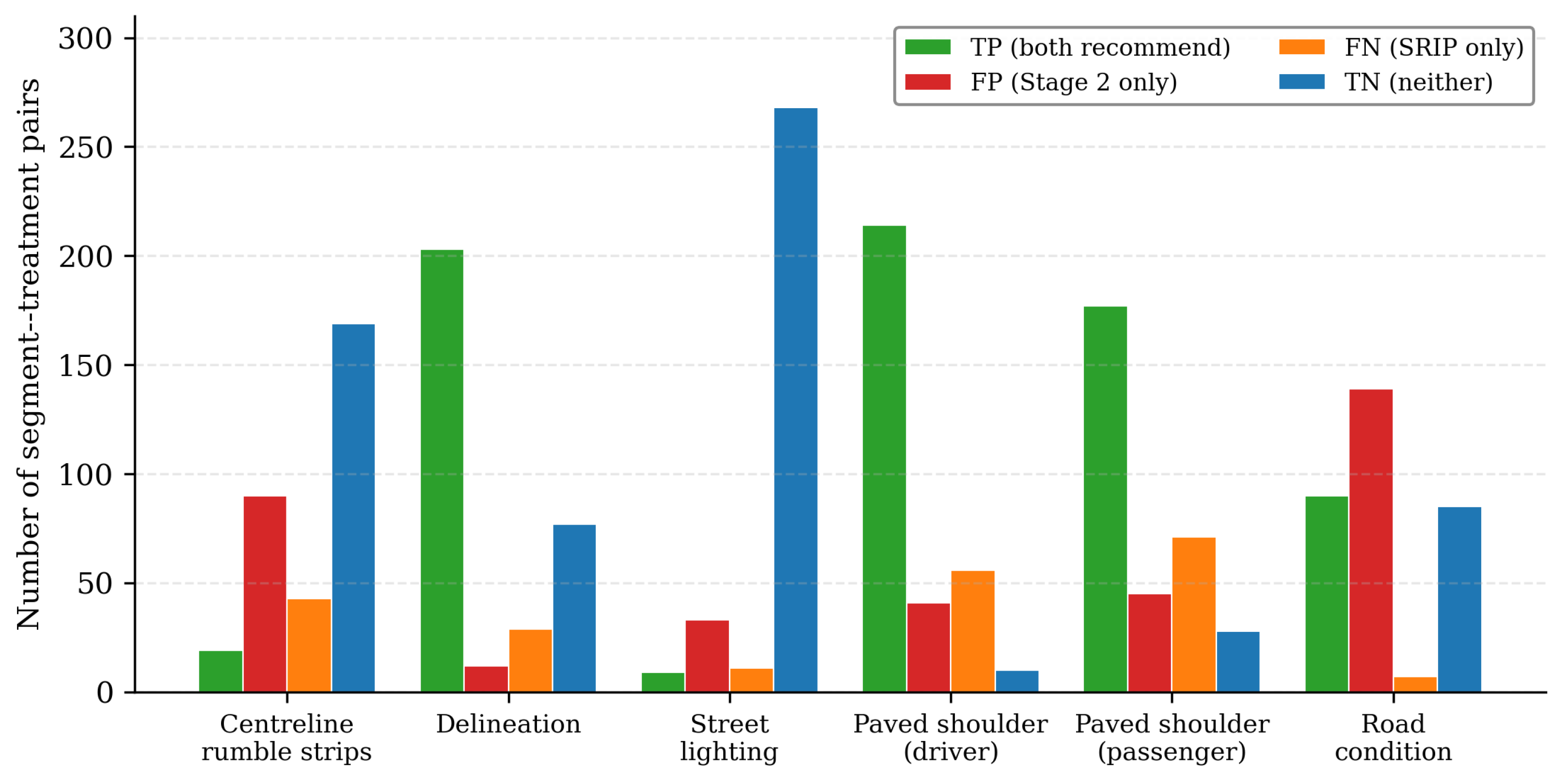
Agreement between the systems is evaluated on the overlap set using three reported summaries. First, we report prescription-level precision, defined on the segment–treatment label table as the proportion of Stage 2-positive pairs that are also positive in SRIP after mapping and deduplication, i.e., . This is an asymmetric measure conditioned on Stage 2’s recommendations; the complementary quantity conditioned on SRIP (recall) is reported alongside it. Second, we compute Cohen’s on the full segment–treatment label table to quantify chance-corrected agreement under the standard definition. Third, we report label-based micro accuracy on the same table. Because and micro accuracy are computed on the full label table, they include true negatives (pairs where both systems abstain for a given treatment class), and micro accuracy can therefore be influenced by the prevalence of such pairs. We interpret prescription-level precision and kappa as the primary agreement measures and treat micro accuracy as supplementary.
Finally, we use the causal forest output to analyse disagreements in more detail, focusing especially on cases where iRAP recommends a treatment in which Stage 2 declines. For all segment–treatment pairs where SRIP recommends a mapped countermeasure but Stage 2 does not recommend the corresponding class, we extract the corresponding estimated association
and summarise disagreement patterns by treatment type. This allows us to check whether the causal forest sees these declined interventions as roughly neutral or as potentially harmful in terms of the modelled FSI. A similar exercise can be performed for false positives to determine where the association model recommends treatments that are not present in the SRIP. The combination of prescription-level precision, classification-style agreement, and association summaries provides a structured way to compare rule-based SRIP recommendations with data-driven prescriptions and to ground the discussion in
Section 5.5.