Effect of Road Markings on Speed Through Curves on Rural Roads: A Driving Simulator Study in Spain

Abstract

Traffic accidents remain a leading cause of mortality worldwide. In Spain, a total of 9666 accidents occurred on curves in 2023, highlighting the need for effective speed management strategies. This study analyses, using a driving simulator, the effectiveness of three low-cost traffic calming measures—checkerboard patterns, red peripheral transverse bars, and red coloured transverse bands—on vehicle speed through curves of varying radii and directions. Additionally, it examines the influence of driver characteristics (age, gender, and experience) and road geometric features (curve radius and direction) on driving behaviour. The simulated road included ten curves with radii ranging from 26 to 190 metres (operating speeds of 30–70 km/h) with traffic calming measures placed at the tangents before the curves. The sample consisted of 48 drivers. Men exhibited faster speeds than women, while younger drivers were faster than seniors. Increased driving experience (annual distances) correlated with higher speeds. Additionally, smaller radii resulted in lower speeds. Regarding the traffic calming measures, significant differences were found mainly where the road markings were placed (tangent) and in the initial phases of the curve. Checkerboard patterns performed better in curves with smaller radii. In contrast, red coloured transverse bands showed the best performance in larger radius curves.

1. Introduction

Traffic accidents are a leading cause of mortality worldwide [1]. Although rural roads witness lower traffic volumes than urban locales, they account for 53% of total crashes [2]. In Spain, a total of 9666 accidents occurred on curves in 2023 [3], highlighting the significant risk posed by these road sections. Analysis of curve accident causes shows that more than half are related to excessive speed and steering errors [4]. Drivers habitually adjust their speed before entering curves based on visual perception, typically reducing speed when curves appear faster and narrower [5,6].

1.1. Effect of Road Markings as Traffic Calming Measures

Traffic calming measures are design strategies that influence driver behaviour, mitigating the adverse effects of vehicle use and enhancing road safety [7,8]. Studying and implementing traffic calming measures is crucial for user safety and comfort. Driving simulators have been used to understand driver, vehicle, and complex driving environments [9]. Numerous studies have examined the effects of physical traffic calming measures (such as transverse rumble strips and road narrowing) on vehicle speed and position in simulated scenarios [10,11]. Other researchers have focused on perceptual traffic calming measures like herringbone markings, dragon’s teeth markings, and optical circles [12,13,14]. Perceptual measures have shown positive results in reducing vehicle speeds [15].

Transverse rumble strips (TRSs) are notable for their effectiveness in reducing vehicle speed. A TRS serve as an acoustic and vibratory warning of a section where a road risk exists further down the road [16]. They are estimated to reduce accidents by 25%. Numerous studies have investigated transverse rumble strips, with findings demonstrating that their implementation before curves or intersections can reduce vehicle speeds by up to 21.9 km/h [10,11,17]. In Spanish regulations, there is a configuration of rumple strips different from the traditional ones, also known as checkerboard patterns (CBPs), which consist of sets of five bars, each one metre long and fifty cm wide, arranged in three rows, with two bars at each end and only one in the middle, forming an “X” [16,18]. The checkerboards were tested with other measures to improve road safety on a hazardous stretch of real road, achieving an average speed reduction of 5.1 km/h immediately after the measures [19].

Peripheral transverse bars (PTBs) are another effective measure. PTBs consist of peripheral bars perpendicular to the road axis with progressively reduced spacing, installed in lanes on both sides [10,20]. Some studies using driving simulators found that these markings reduced vehicle speed by up to 6 km/h in the centre of the curve [12,21]. These results are consistent with the FHWA, which reported reductions of 3 to 5 km/h for standard peripheral transverse bars [20]. Calvi et al. [13] studied white and red PTBs with decreasing spacing between each mark as a vehicle advanced, aiming to affect speed perception, in a curve with an 80 m radius. They found similar results to other studies with white PTBs [12,21]. However, red PTBs reduced speed by up to 12 km/h in the centre of the curve [13].

Coloured transverse bands (CTBs) have also been studied for their impact on vehicle speed. CTBs consist of painted or stamped asphalt concrete bands, usually red, which may or may not include pictograms. Hussain et al. [22] have studied CTBs using driving simulators for pedestrian crossings. CTBs combined with vertical plastic delineators narrowing the lane achieved an approximate speed reduction of 9 km/h compared to a control scenario (no calming measures) [22]. CTBs have also been studied for curve warnings. Some studies implemented two red bands 150 and 75 metres before a curve with a 200 m radius and before entering an urban area [23,24]. Each band had a pattern resembling cobblestones and produced a slight vibration in vehicles crossing them. Results of these showed a speed reduction of 6.7 km/h in the middle of the curve and 22.05 km/h 100 metres before the curve (between the two bands) [24]. In addition to simulator studies, CTBs have been studied on real roads, with studies conducted for the FHWA implementing red-painted CTBs before entering an urban area. Results indicated speed reductions of up to 11.9 km/h in average speeds [25].

Table 1. Summary of different methodologies in the literature.

Authors	Road Markings	Location of Measures	Participants	Driving Simulator	Normality Test	Main Statistical Tests	Post Hoc
Hussain et al. (2021) [8]	Speed limit sign pavement markings	Transition zone	78 (55 M, 23 W)	Yes	Greenhouse-Geisser correction	ANOVA	Not specified
Akbari & Haghighi (2020) [10]	Modified signs, peripheral markings, continuous rumble, hatched design	Transition zone	39 (32 M, 7 W)	Yes	Shapiro–Wilk	RM MANOVA	Bonferroni
Raimondo et al. (2022) [12]	Internal white spaced bands of variable thickness, stripes with variable longitudinal spacing	Highway exit ramp	48 (27 M, 21 W)	Yes	Kolmogorov–Smirnov	Linear Mixed-Effects, Generalized Linear Model	AIC, BIC
Calvi et al. (2019) [13]	Red peripheral transverse bars, white peripheral transverse bars, optical speed bars, chevrons signs	Horizontal curve	38 (26 M, 12 W)	Yes	Kolmogorov–Smirnov	ANOVA	Bonferroni
Martin-Castresana et al. (2024) [14]	Dragon’s teeth markings, red median, broken edge line, green longitudinal speed reduction markings	Pedestrian crossing	60 (34 M, 26 W)	Yes	Kolmogorov–Smirnov	ANOVA	Fisher’s LSD
Babic & Brijs (2021) [15]	Red median, horizontal warning signs	Horizontal curve	43 (25 M, 18 W)	Yes	Greenhouse-Geisser correction	ANOVA	Bonferroni
Matírnez et al. (2013) [19]	Checkerboard patterns	Intersection with horizontal curve	n/a	No	Not applicable	Descriptive statistics	Not applicable
Bobermin et al. (2023) [21]	Peripheral transverse lines starting before the beginning of the curves, peripheral transverse lines starting before the end of the curves	Horizontal curve	56 (all M)	Yes	Not mentioned	Random parameter regression model with heterogeneity in means	Not explicitly mentioned, model accounts for individual and countermeasure variability
Hussain et al. (2023) [22]	Physical narrowing, smart detection-based in-pavement LED light units, variable message sign, zigzag pavement markings, “marking_narrowing”	Pedestrian crossing	58 (49 M, 9 W)	Yes	Not mentioned	McNemar	Bonferroni
Galante et al. (2010) [23]	Transverse rumble strips, transverse optical bars, peripheral transverse bars, roadside fence, coloured brick strip, chicane, gantry	Transition zone	30 (18 M, 12 W)	Yes	Kolmogorov– Smirnov	Kolmogorov–Smirnov, Mann–Whitney	Bonferroni
Montella et al. (2015) [24]	Curve warning sign, flashing beacons, driver feedback sign, transverse rumble strips, coloured transverse strips, transverse rumble strips, dragon’s teeth markings, chevrons, fluorescent sheets, sequentially flashing beacons, coloured median island	Horizontal curve	55 (33 M, 17 W)	Yes	Kolmogorov–Smirnov	ANOVA	Bonferroni

presents a summary of the research methodologies used in previous studies.

1.2. Effects of Driver Characteristics on Speed

Personal characteristics significantly influence driving behaviour. Previous studies have shown that men generally drive faster and perceive traffic violations as less risky, whereas women tend to adopt a more cautious approach [26,27,28]. Age is another important factor, as young drivers account for a higher proportion of road crashes due to their tendency to engage in riskier driving behaviours compared to older drivers [29,30]. Additionally, driving experience enhances vehicle control and risk perception, leading to higher speeds and more confident manoeuvring [31,32,33].

1.3. Effects of Road Geometry on Speed

Although vehicle dynamics such as steering, suspension, tire characteristics, and traction control influence manoeuvrability in curves, road geometry remains a key factor in road safety. Curve radius significantly impacts vehicle speed and driving behaviour, as sharper curves require lower speeds and greater perceptual effort. Previous studies have demonstrated a positive correlation between curvature and accident rates, as sharper curves are associated with increased deceleration and higher accident probability [34,35,36,37]. These curves also lead to reduced operating speeds and increased perceptual demands, as drivers adjust their speed to negotiate tighter turns safely [38,39]. Wang et al. identified speeding, visual distraction, and the geometric characteristics of curves as some of the most critical risk factors contributing to accidents [40]. Road design assumptions often do not align with real driving behaviour, highlighting the need for indicators that reflect actual driver performance, especially when assessing road safety [41]. Analysing actual vehicle speed and acceleration data is critical for understanding real driving behaviour, as idealized design assumptions may not always align with how drivers interact with road geometry [42]. To enhance road safety, increasing curve radius is recommended, as this promotes more consistent speeds and reduces the risk of speed variability [43]. Speed is not constant along curves, challenging traditional design assumptions of steady speeds throughout [24]. This finding highlights potential design inconsistencies and underscores the importance of analysing continuous speed profiles to gain valuable insights for improving road safety and geometric design.

Regarding travel direction, research has yielded mixed results. Some studies have observed significant speed differences between left- and right-hand curves, particularly in the 200 to 400 m radius range, suggesting that directional perception can influence driver behaviour [44]. In contrast, other studies have argued that curve radius is the dominant factor influencing speed, with travel direction having minimal impact [45]. This discrepancy has been attributed to the presence of roadside elements, which can affect perceived safety and influence visual strategies. In addition, previous studies have indicated that drivers tend to drive faster on right-turning than in left-turning curves [46,47].

Previous studies have established that acceptable deceleration rates for safe driving typically range from 0.85 to 1.8 m/s², which translates to variations in speed per metre travelled of 0.102–0.216 m/s/m at 30 km/h and 0.0437–0.0926 m/s/m at 70 km/h [48,49,50,51]. Sudden and excessive deceleration should be minimised not only for safety reasons but also to reduce pavement wear and maintenance needs [52]. Several studies have highlighted the relationship between crash frequency and abrupt driving manoeuvres, particularly harsh braking and harsh acceleration, as they indicate loss of vehicle control or late reaction to road conditions [53].

1.4. Objective of the Study

This study aims to evaluate the effectiveness of traffic calming measures on vehicle speed through curves of varying radius and direction and analysing the influence of driver characteristics on speed. For this, three traffic calming measures (road markings)—CBPs, red PTBs, and red CTBs—have been selected. Rumple strips forming an “X” or CBPs are commonly used in Spain, yet their effects remain under-researched. PTBs and CTBs have demonstrated significant speed reductions in previous studies, often outperforming other measures. This study was carried out using a driving simulator, allowing for a controlled environment, safe testing of various scenarios, and precise speed measurements.

2. Methodology

2.1. Road Design

The horizontal alignment consisted of 10 curves and 11 large tangents (Figure 1). The radii of circular curves were designed to achieve a specific operating speed (30, 40, 50, 60, or 70 km/h) following Spanish regulations [54]. The tangent between each curve was 500 metres long, a distance considered sufficient to ensure the independence of each curve [54]. The tangent before the first curve and after the last one was 600 metres long, allowing drivers to accelerate from a stationary position at the start and decelerate comfortably at the end of the experiment. The deflection angle was always 90 gon. There were spirals before and after each circular curve (according to Spanish regulations). The vertical alignment was designed with a 0% grade to exclude it as a variable in the study. The cross-section was also designed according to Spanish regulations and consisted of two 3.5 m lanes, a 1 m shoulder, 0.75 m benches, and superelevation of 7%. The friction coefficient considered was 0.97, a typical value for dry pavement in good condition with well-maintained tyres.

2.2. Design of Road Markings

Four scenarios (or alternatives) were created to study the effect of traffic calming measures on speed (Figure 2):

• The base scenario (Alt. 0) (without traffic calming measures) that serves as a reference to assess the effectiveness of the traffic calming measures by comparing it with the other scenarios.
• Scenario 2 (Alt. 1): checkerboard patterns (CBPs).
• Scenario 3 (Alt. 2): red peripheral transverse bars (PTBs).
• Scenario 4 (Alt. 3): red coloured transverse bands (CTBs).

All traffic calming measures begin 200 metres before the end of the tangent and the start of the spiral. The same vertical signs were used for all alternatives. At the beginning of each tangent, a sign indicating the maximum speed (90 km/h) was placed. Additionally, 200 metres before each curve, a double sign was positioned, displaying the recommended maximum speed and the direction of the curve (Figure 2).

In Alt. 1 (Figure 2), CBPs are implemented, designed according to the M-8.3 marking from the draft of the new Spanish road marking standard. The configuration of these consists of sets of 5 bars, each 1 metre long and 50 cm wide, arranged in 3 rows, with 2 bars at each end and only 1 in the middle, forming an “X” [16,18]. CBPs generate noise and vibration in vehicles as they pass over them. Their longitudinal arrangement aims to influence drivers’ perception of speed by progressively reducing the spacing between each CBP. The spacing should correspond to the distance a vehicle travels in one second. As the vehicle advances, the spacing is reduced in intervals corresponding to a 10 km/h decrease in design speed until reaching the curve’s design speed. The sequence concludes with three sections spaced according to the final speed (see example in Figure 3). The distance between the last CBP and the start of the curve must be greater than 50 metres and exceed the stopping distance.

Alt. 2 (Figure 2) uses red PTBs based on the literature [13]. Red bars measuring 45 × 45 cm are placed on both sides of the lane, with their spacing progressively decreasing as the vehicle advances [55]. Since five different design speeds were considered, a specific configuration was developed for each case. Figure 4 presents the design for curves C7 and C8 (70 km/h), proportionally adjusted to 200 metres.

In Alt. 3 (Figure 2), red CTBs are implemented with a pattern designed to imitate brick pavers on the bituminous concrete, generating noise and vibration as vehicles cross them. Two bands, each 5 metres long and 3.25 metres wide, were used. This design is like those proposed in the literature but with different spacing [23,24]. The first band was placed 200 metres before the curve and the second 100 metres before. This configuration remained unchanged across all curves, regardless of their specific design speed (Figure 5).

2.3. Experimental Design

The driving simulator is located at the Road Laboratory of the Escuela Técnica Superior de Ingenieros de Caminos, Canales y Puertos (Universidad Politécnica de Madrid). The simulator consists of a computer with three 32-inch screens and a set consisting of a steering wheel, pedals, and a gear lever (Figure 6). This simulator has been validated in previous speed studies [56].

A total of 48 volunteers performed the driving tests in the simulator.

Table 2. Characteristics of the driver sample (percentages).

Gender		Age (years)			Annual Experience (km/year)
Male (M)	Female (W)	18–24 (Y)	25–49 (MA)	>50 (S)	<10,000 (G1)	10,000–20,000 (G2)	>20,000 (G3)
54.2	45.8	8.3	50	41.7	39.6	47.9	12.5

summarizes the distribution of the sample by age (young, middle-aged, senior), gender (male, female), and annual driving experience (<10,000, 10,000–20,000, >20,000 km/year). These ages and genders provide a mirroring of Spanish drivers [57]. The average age was 42.9 years old (standard deviation = 16.0, range = 20–73 years). The average driving license antiquity was 22.4 years.

All participants were volunteers, and they did not receive any remuneration. None of them were under the supervision or authority of the research team. All were informed of the research objectives and the conditions of the trial before it commenced and filled out a preliminary questionnaire. The data were processed anonymously. The study does not include details of ethnic origin, political opinions, religious beliefs, physical or mental health issues, trade union affiliation, or sexual life.

For the experimental tests, the procedure involved four stages designed to ensure complete data collection on participants’ driving experiences. The first stage lasted approximately 1 min, during which the simulator controls were explained to each participant. In the second stage, participants completed a 3-min training drive within the simulator to familiarize themselves with the controls. In the third stage, each participant drove four scenarios (three scenarios with measures and one without) in random order to exclude potential learning effects, each lasting 6 to 8 min, followed by a 3-min rest period. Finally, in the fourth stage, after all driving trials, participants completed an evaluation questionnaire to gather information on their driving preferences and any issues experienced, such as nausea or fatigue. The total experimental procedure lasted 45 to 55 min per participant, including breaks.

2.4. Data Analysis

Ten control points were defined to measure participants’ speeds in curves and tangents (Figure 7). Points P1, P2, and P10 are located on the tangent before and after each curve, while the others are situated within the curve (spiral and circular curve). As the case study consisted of 10 curves separated by tangents, speeds were analysed at a total of 100 points on the road.

The data analysis followed a structured approach to assess the impact of different road marking alternatives on driver behaviour, considering various influencing factors. First, the normality of the data was verified using the Kolmogorov–Smirnov test to determine whether parametric statistical tests were appropriate. After confirming normality, a parametric analysis of variance (ANOVA) was performed. Then, ten predefined points within each of the ten curves analysed were grouped into homologous study points. For example, the first points of each curve were classified as the first homologous point, the second points as the second homologous point, and so on. This approach allowed for comparative analysis across different phases of the road network. An ANOVA was conducted at these points, comparing the means of the groups defined by the different levels of the influencing factors on speed: gender (M: Men, W: Women), age (Y: 18–24 years, MA: 25–49 years, S: >50 years), annual driving experience (G1: <10,000 km/year, G2: 10,000–20,000 km/year, G3: >20,000 km/year), road marking alternative (Alt. 0: Base scenario, Alt. 1: CBPs, Alt. 2: Red PTBs, Alt. 3: Red CTBs), curve radius (R26: 26 m, R50: 50 m, R85: 85 m, R130: 130 m, R190: 190 m), and driving direction (L: Left Turn, R: Right Turn). Significant differences were further examined through Fisher’s Least Significant Difference (LSD) post-hoc test (Appendix A). Additionally, speed profiles at the homologous points were analysed to assess how different variables influenced speed behaviour. A confidence interval of 95% was used for all statistical tests.

The analysis then focused on the relationship between road marking alternatives and road geometry (curve radius and driving direction). Separate ANOVA tests and Fisher LSD post-hoc tests were conducted to identify significant effects, while speed profiles for each curve were examined to observe how different markings influenced speed trends along the approach and within the curve. Speed variation per metre of travel was also analysed between study stations to quantify the impact of each alternative on speed reduction dynamics.

3. Results

First, Kolmogorov–Smirnov normality tests were conducted on the speed data distributions, confirming that they followed a normal distribution. This test compares the empirical distribution of the sample data with a normal distribution to determine if there are significant deviations. A p-value greater than 0.05 indicates that the null hypothesis of normality cannot be rejected, suggesting that the data follow a normal distribution.

Table 3. Results of the Kolmogorov–Smirnov normality test for each curve (p-value > 0.05 indicates normal distribution).

Curves	P1	P2	P3	P4	P5	P6	P7	P8	P9	P10
C1	0.26	0.19	0.19	0.71	0.69	0.75	0.85	0.87	0.38	0.99
C2	0.78	0.18	0.55	0.56	0.87	0.76	0.95	0.95	0.87	0.77
C3	0.72	0.71	0.98	0.9	0.81	0.52	0.24	0.63	0.79	0.89
C4	0.57	0.44	0.33	0.85	0.45	0.57	0.34	0.31	0.88	0.89
C5	0.11	0.52	0.47	0.3	0.46	0.22	0.24	0.32	0.78	0.76
C6	0.27	0.45	0.8	0.83	0.55	0.69	0.78	0.87	0.89	0.89
C7	0.31	0.61	0.82	0.9	0.99	0.87	0.71	0.62	0.49	0.55
C8	0.29	0.58	0.07	0.99	0.82	0.58	0.46	0.64	0.75	0.8
C9	0.06	0.09	0.49	0.67	0.68	0.65	0.65	0.65	0.88	0.8
C10	0.97	0.51	0.65	0.86	0.83	0.87	0.87	0.93	0.99	0.92

presents the results for each curve. After confirming normality, a parametric ANOVA was performed.

3.1. Effects of Geometric and Personal Factors on Speed

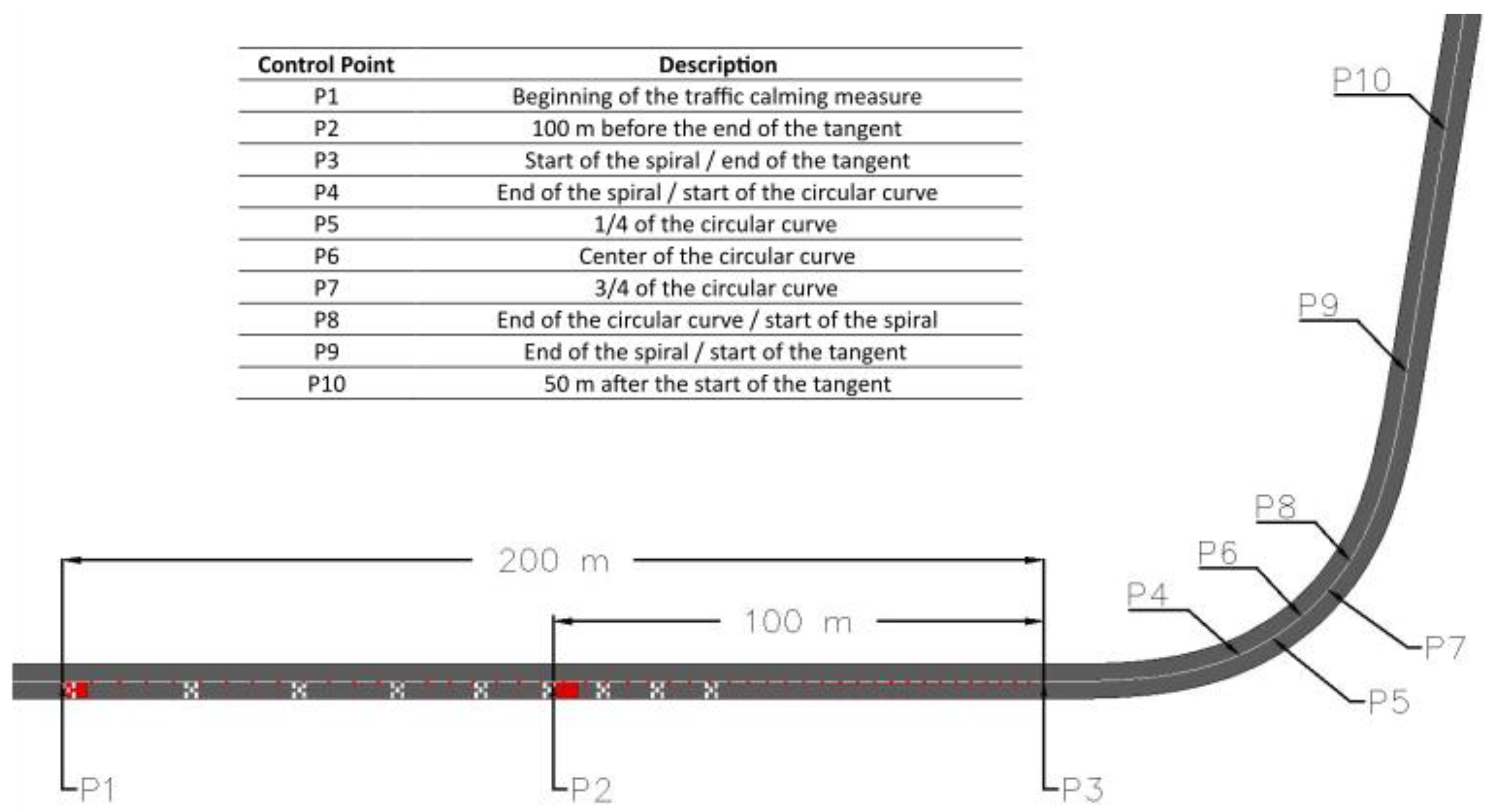
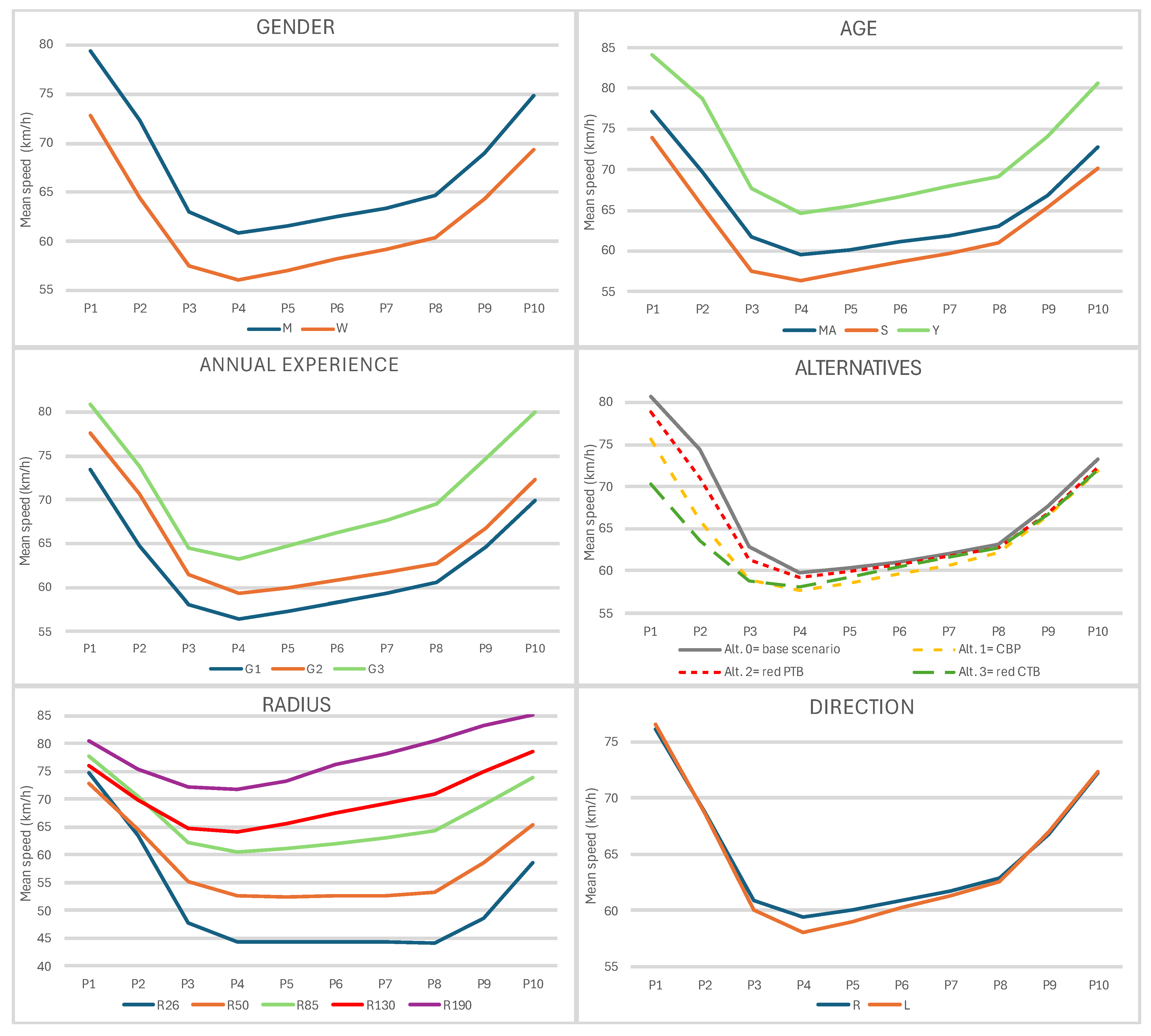
Figure 8 presents the mean speed profiles (km/h) across ten homologous points (P1–P10), representing different phases of the curve, for six analysed factors. These plots allow for a comparative analysis of how each factor influences speed variation along the trajectory. The results indicated that gender, age, annual experience, and radius exhibited notable differences between groups, while direction showed minimal variation. The shape of the speed curves suggested a common deceleration and acceleration pattern across all factors, with the lowest mean speed occurring at P4, which corresponded to the end of the spiral and the beginning of the circular curve. The greatest overall speed reduction took place in the approach phase.

Table 4. ANOVA results (p-value) for six factors at homologous points of the curve.

Factor (ANOVA)	P1	P2	P3	P4	P5	P6	P7	P8	P9	P10
Gender	<0.01	<0.01	<0.01	<0.01	<0.01	<0.01	<0.01	<0.01	<0.01	<0.01
Age	<0.01	<0.01	<0.01	<0.01	<0.01	<0.01	<0.01	<0.01	<0.01	<0.01
Experience	<0.01	<0.01	<0.01	<0.01	<0.01	<0.01	<0.01	<0.01	<0.01	<0.01
Alternative	<0.01	<0.01	<0.01	<0.05	0.19	0.41	0.54	0.80	0.72	0.34
Radius	<0.01	<0.01	<0.01	<0.01	<0.01	<0.01	<0.01	<0.01	<0.01	<0.01
Direction	0.49	0.93	0.20	0.02	0.08	0.30	0.52	0.73	0.74	0.84

shows the ANOVA results for the six factors along the ten homologous points. Notably, while some factors, such as gender, age, and annual experience, consistently yielded highly significant results (p = <0.01 across all points), others, such as alternative and direction, exhibited more variability, suggesting differential effects along the curve. To complement these results,

Table 5. ANOVA effect sizes (η², percentage) for six factors at homologous points of the curve.

Factor (ANOVA)	P1	P2	P3	P4	P5	P6	P7	P8	P9	P10
Gender	6.1	7.7	4.2	3.4	2.8	2.2	2.0	1.8	2.2	4.0
Age	4.4	6.5	5.0	3.4	2.8	2.4	2.3	1.9	2.2	4.0
Experience	3.8	5.7	2.7	2.9	3.1	3.0	3.0	3.0	4.0	5.0
Alternative	8.9	8.8	1.6	0.4	0.2	0.2	0.1	0.1	0.1	0.2
Radius	3.8	9.2	39.8	53.9	58.6	62.2	64.1	65.7	61.7	44.9
Direction	0.0	0.0	0.1	0.3	0.2	0.1	0.0	0.0	0.0	0.0

presents the effect sizes (η²) in percentage form, providing insight into the practical significance of these differences. While statistical significance indicates whether an effect exists, the η² values help assess its magnitude. Radius is the dominant factor influencing speed variation, with consistently high effect sizes across the curve.

The ANOVA analysis of the gender factor showed statistically significant differences at all homologous points (P1–P10, p < 0.01, Table 4), indicating that gender consistently influenced speed. Male drivers maintained higher speeds than female drivers across all phases of the trajectory. The greatest difference between both genders occurred at P2, where male drivers were 7.97 km/h faster than female drivers (Figure 8). This point was located 100 metres before the end of the straight section, where traffic calming measures were implemented.

Speed was significantly influenced by the driver’s age, with statistically significant differences at all homologous points (P1–P10, p < 0.01, Table 4). The Fisher LSD post hoc test confirmed these differences across all age groups (Y: 18–24 years, M: 25–49 years, S: ≥50 years) at every point, except at P9 (start of the second tangent), where no significant difference was found between M and S drivers (Appendix A). Younger drivers (Y) maintained the highest speeds, older drivers (S) exhibited the lowest, and the middle-aged group (M) fell in between, with average speed differences of 6.55 km/h between Y and M, 9.37 km/h between Y and S, and 2.83 km/h between M and S. The greatest difference between age groups occurred at P2, where Y drivers exceeded S drivers by 13.31 km/h (Figure 8).

Annual driving experience influenced speed, with statistically significant differences at all homologous points (P1–P10, p < 0.01, Table 4). The Fisher LSD post hoc test confirmed significant differences between all experience levels (Appendix A), with higher-annual distance drivers maintaining consistently higher speeds, while those with lower annual distance adopted a more cautious approach, showing average speed differences of 3.01 km/h (G2–G1), 8.25 km/h (G3–G1), and 5.16 km/h (G3–G2) (Figure 8). The greatest difference occurred between G1 and G3 drivers at P10 (50 m after the start of the tangent), where G3 drivers exceeded G1 by 10.12 km/h.

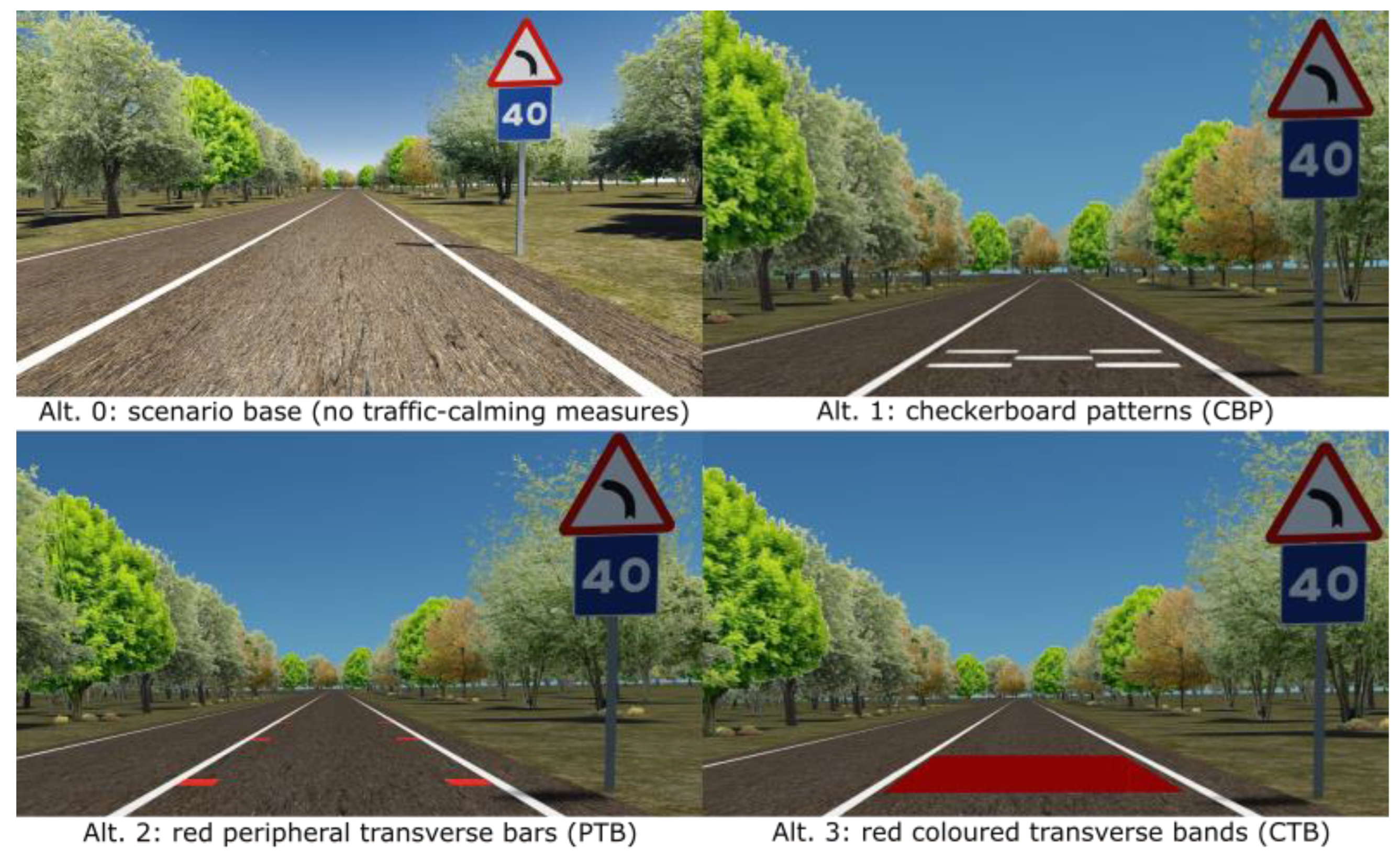
Speed was significantly influenced by the tested alternative, with differences observed at the initial segments of the trajectory. Statistically significant variations were found from P1 to P3 (p = <0.01) and at P4 (p = <0.05) (Table 4), confirming that the road markings affected driver behaviour before the curve but lost relevance beyond this point. The Fisher LSD post hoc analysis confirmed that the impact varied across alternatives (Appendix A). The CBPs (Alt. 1) consistently reduced speed from P1 to P5 compared to the base scenario, with the greatest reduction at P2, where drivers lowered their speed by 8.4 km/h (Figure 8). On average, this alternative resulted in a 2.75 km/h lower speed than the base scenario. The red PTBs (Alt. 2) exhibited significant differences only at P1 and P2, indicating an early but limited effect, with their maximum reduction also at P2 (3.36 km/h) and an overall average reduction of 1.08 km/h. The red CTBs (Alt. 3) produced the strongest impact on speed reduction, with significant effects extending from P1 to P4, reaching a peak at P2, where the speed decrease was 10.83 km/h. This alternative maintained an average reduction of 3.18 km/h.

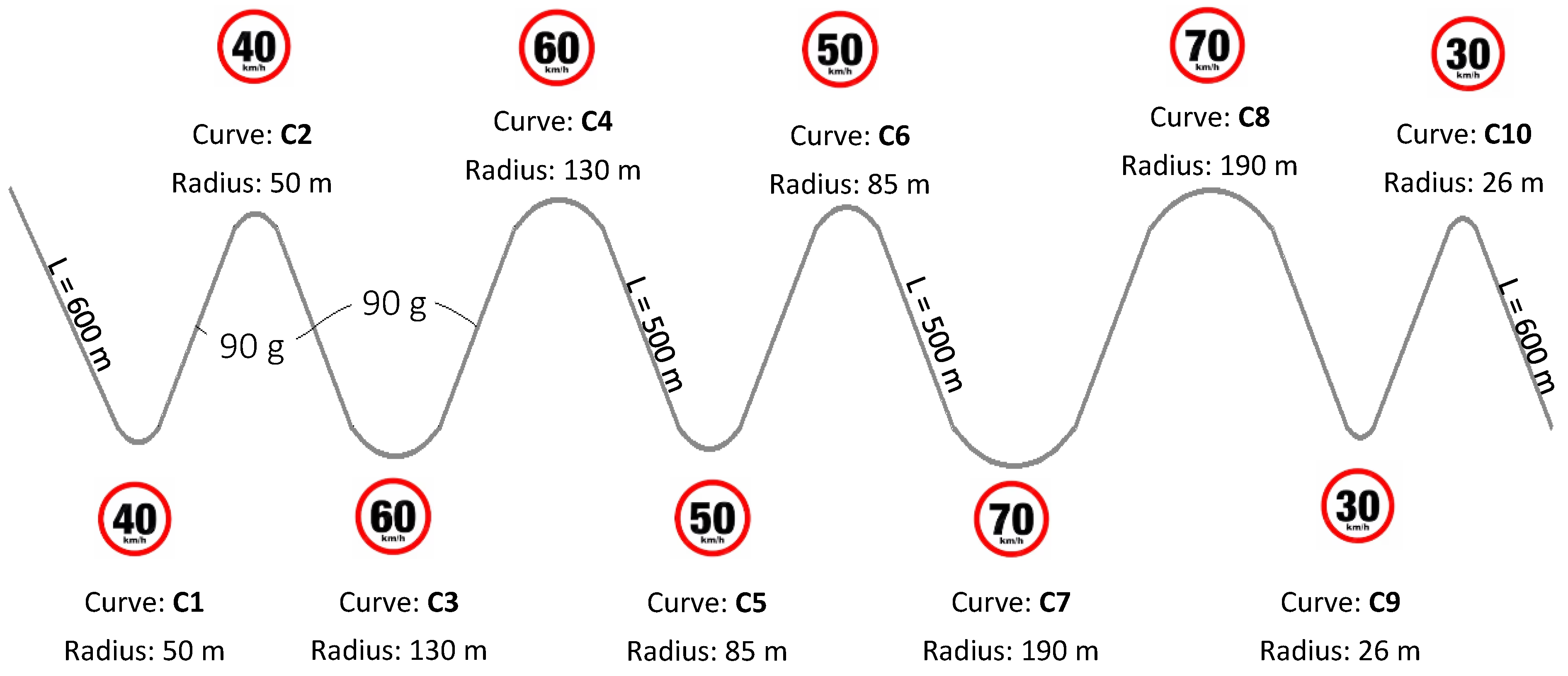
Speed was significantly influenced by curve radius, the dominant factor in speed variation (Table 5), with p-values of <0.01 at all homologous points (Table 4). Smaller radii were associated with lower vehicle speeds, as sharper curves imposed greater constraints on driving dynamics. However, the differences in speed due to radius were less pronounced at the initial points closer to the straight section (Figure 8), indicating that the effect of curve geometry on speed became more evident as drivers progressed further into the curve. The post hoc analysis confirmed significant differences in speed across all radius comparisons at nearly every homologous point (Appendix A).

Travel direction showed minimal influence on speed, with no statistically significant differences at most homologous points, except at P4 (end of the spiral/start of the curve), where a p-value of 0.02 indicated slightly higher speeds in the rightward direction (Table 4). Despite this isolated difference of 1.33 km/h (Figure 8), the overall impact of travel direction appeared negligible compared to the other factors analysed.

3.2. Effects of Road Markings by Curve Radius

Table 6. ANOVA results (p-values) for the alternative factor across curve pairs grouped by radius.

ANOVA	P1	P2	P3	P4	P5	P6	P7	P8	P9	P10
R = 26 m (C9 and C10)	<0.01	<0.01	0.50	0.56	0.56	0.56	0.56	0.31	0.69	0.41
R = 50 m (C1 and C2)	0.01	<0.01	0.04	0.24	0.25	0.26	0.29	0.78	0.63	0.45
R = 85 m (C5 and C6)	<0.01	<0.01	0.01	0.21	0.29	0.34	0.46	0.62	0.72	0.58
R = 130 m (C3 and C4)	<0.01	<0.01	<0.01	0.06	0.21	0.46	0.65	0.66	0.67	0.76
R = 190 m (C7 and C8)	<0.01	<0.01	<0.01	0.02	0.40	0.91	0.95	0.95	0.99	0.98

presents the results of the ANOVA analysis for the alternative factor, comparing homologous speed points (P1–P10) between pairs of curves grouped by radius. Given that the direction factor did not show significant effects (Table 4), curves were analysed in pairs based on their radius to better assess the impact of alternatives on speed variation. Statistically significant differences (p < 0.05) were observed mainly in the initial phases (P1–P3), where all curve pairs exhibited notable differences (Table 6). However, as drivers progressed through the curve, significance decreased, and from P5 onwards, differences became largely non-significant.

Figure 9 presents the analysis of speed behaviour across the five studied curve radii grouped in pairs. The left column displays the mean speed profiles (km/h) for each alternative at the homologous points (P1–P10), allowing for direct comparisons of how the different traffic calming measures influenced speed reduction along the trajectory in each curve. The right column illustrates the variation in speed per metre travelled (m/s/m) at the stations where the previous ANOVA results identified statistically significant differences (P1–P4, Table 4). This visualization enabled a more detailed assessment of the rate of speed variation per metre travelled and how it varied between alternatives in the early phases of the curve approach.

C9 and C10, the smallest curves in the study with radii of 26 metres, showed significant differences in the early segments according to the ANOVA results, with low p-values at P1 and P2 (p < 0.01, Table 6). These differences decreased from P3 onward. The speed profile (Figure 9, left) revealed that red CTBs resulted in the greatest speed reductions at the first two points. At these points, both red CTBs and CBPs showed statistically significant differences according to the Fisher LSD test (Appendix A). From the third point onwards, the reduction was comparable across the three alternatives. While red PTBs followed an intermediate pattern, they resulted in a speed reduction of only 1.5 km/h before the start of the curve. Regarding speed variations per metre travelled (Figure 9, right), CBPs started at 0.034 m/s/m in P1–P2, reached a maximum of 0.038 m/s/m in P2–P3, and declined to 0.024 m/s/m in P3–P4. Red PTBs followed a similar pattern but with higher values, beginning at 0.035 m/s/m, rising to 0.050 m/s/m, and reducing to 0.032 m/s/m in the final section. Finally, red CTBs showed the least variation, with values of 0.025 m/s/m in P1–P2, a slight increase to 0.032 m/s/m in P2–P3, and a decrease to 0.025 m/s/m in P3–P4, indicating a more stable speed transition.

For curves with a 50 m radius (C1 and C2), the ANOVA revealed statistically significant differences in the early segments of the trajectory (p-values < 0.05 at points P1, P2, and P3, Table 6). From P4 onwards, p-values increased, suggesting that the effect of the alternatives diminished as vehicles progressed through the curve. The speed profile showed a progressive reduction at the initial sampling points, reaching a minimum at P4, where the average speed became similar across all alternatives (Figure 9, left). However, differences were notable before entering the curve. Red CTBs produced the greatest speed reduction at P2 (9.73 km/h), while CBPs also led to a significant decrease compared to the base scenario, though to a lesser extent (8.8 km/h at P2). Red PTBs had an intermediate effect, with moderate reductions at P2. On average, across all homologous points, compared to the base scenario, CBPs reduced speed by 2.97 km/h, red PTBs by 1.00 km/h, and red CTBs by 2.62 km/h. Notably, CBPs showed statistically significant differences at P2 and P3 according to the Fisher LSD test, while red CTBs exhibited significant differences at P1, P2, and P3 (Appendix A). The speed variation per metre travelled (Figure 9, right) supported these findings. CBPs exhibited progressively smaller variations in speed as the hazard was approached, with values of 0.03 m/s/m in P1–P2, 0.023 m/s/m in P2–P3, and decreasing to 0.014 m/s/m in P3–P4. Red PTBs started at 0.022 m/s/m in P1–P2, increased to 0.027 m/s/m in P2–P3, and then decreased to 0.023 m/s/m in P3–P4. Red CTBs showed the least variation among the three, with values of 0.026 m/s/m in P1–P2, a reduction to 0.016 m/s/m in P2–P3, and a further gradual decrease to 0.013 m/s/m in P3–P4, reflecting uniform behaviour and less fluctuation in speed, like CBPs.

For curves C5 and C6 (85 m radius), the ANOVA results showed a statistically significant impact of the road marking alternatives between P1 and P3 (Table 6). The speed profile (Figure 9, left) revealed that all alternatives led to a reduction in speed before the curve, though with varying intensity. Red CTBs caused the greatest speed reduction at P2 (9.36 km/h), indicating an earlier and stronger driver response. CBPs followed a similar pattern but with a slightly lesser effect (9.13 km/h), while red PTBs remained closer to the base scenario, with a reduction of only 3.2 km/h 100 m before entering the curve. CBPs and red CTBs showed statistically significant differences at P1, P2, and P3 according to the Fisher LSD test (Appendix A). The speed variations per metre travelled provided additional insights (Figure 9, right). CBPs exhibited a speed variation of 0.026 m/s/m in P1–P2, decreasing to 0.019 m/s/m in P2–P3 and further declining to 0.006 m/s/m in P3–P4. The red PTBs started at 0.024 m/s/m in P1–P2, reached a peak of 0.027 m/s/m in P2–P3, and then decreased to 0.012 m/s/m in P3–P4. Meanwhile, the red CTBs showed the least variation, beginning at 0.012 m/s/m in P1–P2, increasing slightly to 0.015 m/s/m in P2–P3, and reducing to 0.004 m/s/m in P3–P4.

For curves with a 130 m radius (C3 and C4), the ANOVA results showed that road marking alternatives had a statistically significant impact mainly in the early trajectory segments, with p-values remaining low until P4 with a marginal value of 0.06 (Table 6). From P5 onwards, the effect diminished as p-values increased. The speed profile (Figure 9, left) highlighted a clear differentiation between alternatives before reaching the lowest speed point (P4). Red CTBs produced the greatest speed reduction on the approach, with a sharper drop at P2 compared to the base scenario (13 km/h). CBPs also caused a notable reduction, though smaller than red CTBs, while red PTBs remained closer to the base scenario. Post hoc analysis revealed statistically significant differences for the following: CBPs from P1 to P4, red PTBs at P2, and red CTBs from P1 to P3 (Appendix A). The speed variation per metre travelled (Figure 9, right) supported these findings. CBPs exhibited a decrease in speed variation, starting at 0.025 m/s/m in P1–P2, dropping to 0.012 m/s/m in P2–P3, and continuing to decline to 0.002 m/s/m in P3–P4. Red PTBs began at 0.016 m/s/m in P1–P2, maintained the same value in P2–P3, and decreased to 0.004 m/s/m in P3–P4. Red CTBs started at 0.014 m/s/m in P1–P2, decreased to 0.003 m/s/m in P2–P3, and further dropped to −0.004 m/s/m in P3–P4, indicating a consistent speed variation per metre travelled, like the CBPs.

Among the studied curves, C7 and C8 had the largest radius (190 m), and the ANOVA results showed statistically significant differences in speed reductions across the road marking alternatives, particularly in the approach phase (Table 6). The speed profile (Figure 9, left) showed that red CTBs caused the greatest speed reduction at 100 m before the curve (12.32 km/h), which is considerably less than the 22.05 km/h reduction observed by Montella [15], followed by CBPs, which showed a noticeable decrease at the same point (P2, 7.5 km/h). Red PTBs remained closer to the base scenario, with a less pronounced effect on speed reduction. Post hoc Fisher LSD analysis revealed statistically significant differences for CBPs from P1 to P3 and for red CTBs from P1 to P4 (Appendix A). In speed variation per metre travelled (Figure 9, right), CBP started at 0.018 m/s/m in P1–P2, progressively declined to 0.005 m/s/m in P2–P3, and further dropped to −0.001 m/s/m in P3–P4. Red PTBs began at 0.012 m/s/m in P1–P2, maintained the same value in P2–P3, and decreased to 0.005 m/s/m in P3–P4. Red CTBs exhibited a greater reduction in speed, starting at 0.013 m/s/m in P1–P2, decreasing to 0.001 m/s/m in P2–P3, and finishing at −0.006 m/s/m in P3–P4.

4. Discussion

The observed deceleration and acceleration trends on the studied road align with established road safety findings. Previous studies have reported that drivers tend to reduce their speed more significantly before encountering a perceived hazard, such as a curve or crossing, but then increase their speed once they have passed the critical area [5,6]. In this study, the lowest speeds were recorded at P4, marking the transition from the spiral to the circular curve, reinforcing the idea that drivers anticipated the risk in advance and adjusted their speed accordingly.

Gender-based differences in speed modulation can be attributed to variations in risk perception, driving experience, or decision-making strategies when approaching a curve. Female drivers exhibited a more cautious approach, which is consistent with previous studies indicating that men generally drive faster and perceive traffic hazards as less risky, while women tend to adopt more conservative driving behaviours [26,27,28]. The significant speed gap observed at P2 suggests that male drivers may delay speed reduction when approaching a potential hazard, while female drivers adjust their speed earlier in anticipation.

The analysis confirms the well-established relationship between age and driving behaviour, with younger drivers exhibiting riskier speed patterns while older drivers display more cautious profiles. The largest speed gap at P2 suggests that younger drivers delay deceleration more than older drivers when approaching a hazard, a behaviour that may contribute to their higher levels of crash involvement. These findings align with previous research indicating that younger drivers tend to engage in riskier driving behaviours, which correlates with their overrepresentation in road crashes [29,30].

Driving experience plays a key role in speed modulation, with more experienced drivers demonstrating greater confidence in handling curves and transitions. This behaviour is likely linked to differences in risk perception and familiarity with vehicle dynamics, with lower annual distance drivers adopting a more conservative approach. These findings align with previous studies indicating that increased driving experience enhances vehicle control and hazard anticipation, resulting in higher speeds and more confident manoeuvring [31,32,33].

Road markings primarily influence driver behaviour before entering a curve, aligning with previous findings that reported significant speed reductions at the initial points along a straight segment prior to a curve [11,15,24,52]. The observed reduction aligns with the placement of the markings, reinforcing the idea that drivers respond to visual stimuli well in advance of a perceived hazard. However, the absence of significant effects within the curve itself indicates that once drivers are engaged in navigating the curve, the influence of the markings diminishes. The comparison of alternatives highlights distinct behavioural responses: CBPs maintained a prolonged reduction, while the red CTBs induced the most substantial decrease in the early phase. This suggests that different treatments may serve varying objectives, with CBPs fostering a gradual adjustment in speed and red CTBs prompting a sharper initial response.

The results reinforce the well-established relationship between curve radius and speed, demonstrating that as drivers enter a curve, their speed adaptation is increasingly dictated by geometric constraints. This pattern highlights the role of curve design in shaping driver response and supports the notion that increasing curve radius enhances road safety by promoting consistent speeds. Furthermore, the results confirm that speed is not constant along curves, revealing potential design inconsistencies that could contribute to abrupt speed variations and increased crash risk [24]. These findings align with previous research showing that sharper curves reduce operating speeds and influence driving behaviour [38,39].

Speed variations were more influenced by curve geometry than by travel direction [24]. These findings were consistent with research concluding that curve radius predominantly affected vehicle speed choice, whereas travel direction had minimal impact [45]. Although some studies have reported speed differences between left- and right-hand curves [46,47], the results of this study only showed a significant difference at P4 (the end of the spiral and the start of the circular curve).

Curves with a radius of 26 metres exhibited a distinct speed reduction pattern in the early segments, particularly with red CTBs and CBPs. These results contrast with those of Katz [55], who reported a 28% speed reduction with red PTBs before a curve with a 31-metre radius. The greater reduction observed in Katz’s study is likely due to differences in curve perception and driving behaviour rather than the radius itself. In this research study, red CTBs and CBPs led to reductions of less than 5% in the centre of the curve, indicating that while these measures influence approach speeds, their impacts within the curve are more moderate.

Curves with a radius of 50 metres showed progressive speed reductions before entering the curve, particularly with red CTBs and CBPs. In the P2–P3 segment, CBPs and red CTBs exhibited lower speed variations per metre travelled rate compared to the previous segment, suggesting that drivers adjusted their speed earlier on the approach. This progressive adaptation to the road markings may indicate beneficial effects in terms of anticipation and driving comfort.

Curves with an 85-metre radius exhibited a clear speed reduction pattern before the curve, with red CTBs and CBPs being the most effective treatments. Compared to previous studies, which reported reductions of approximately 15 km/h before a curve of similar radius [13], the results in this study indicate a smaller but still notable speed decrease. The earlier response triggered by CBP markings suggests that they enhance driver anticipation, whereas the red CTB bands produced a delayed but more intense speed variation per metre travelled.

For curves with a 130-metre radius, speed reduction was most pronounced in the early trajectory segments, particularly before reaching the lowest speed point at P4. The fact that red CTBs caused the sharpest reduction at P2 suggests that transverse bands play a key role in encouraging early deceleration. CBPs also proved effective but to a lesser extent, while red PTBs had a minimal impact compared to the base scenario. The findings align with the existing literature, which suggests that transverse bands enhance driver awareness and promote earlier speed adaptation [23]. Additionally, the negative speed variation observed in P3–P4 for red CTBs implies that drivers had already completed most of their deceleration before entering the curve, leading to a smoother and more stable speed adjustment.

For the largest studied curves (190-metre radius), the effectiveness of road markings in reducing speed was primarily observed in the approach phase, particularly for red CTBs and CBPs. The observed reduction of 12.32 km/h at 100 metres before the curve with red CTBs is considerably lower than the 22.05 km/h reduction reported by Montella at the same location [24].

The obtained speed variation per metre values for all alternatives fall within safe and comfortable ranges according to the previous literature [48,49,50,51].

5. Conclusions

Significant differences were observed across all curve phases based on gender, age, annual driving experience, and curve radius. Radius is the dominant factor influencing speed variation, as shown by its consistently high effect sizes across the curve. Men exhibited faster speeds than women, while younger drivers were faster than seniors. Increased driving experience correlated with higher speeds. Additionally, smaller radii resulted in lower speeds, with less noticeable differences observed in the tangent phases. No significant differences were found between right- and left-hand curves, except at the point located at the end of the spiral and the beginning of the straight section.

In the marking alternatives tested, significant differences were observed in the tangent sections leading up to the initial phases of the curve. These differences were most pronounced with comparison of the CBPs and red CTBs to the baseline scenario. In both small and large radius curves, significant differences were observed in the tangent section preceding the curve. However, in large radius curves, these differences extend further into the curve, whereas in small radius curves, they are confined to the initial section.

CBPs perform better in curves with a smaller radius, particularly those with operating speed of 40 and 50 km/h. In contrast, their effectiveness decreases in larger-radius curves. Additionally, a consistent speed variation per metre travelled is observed across the three studied zones in all curves, except for the 30 km/h curve.

The red PTB markings performed the least effectively among the three measures, despite their presence extending to the end of the straight section. This may be attributed to the lack of noise or texture in the road markings, which potentially limited their ability to influence driver behaviour. In comparison to CBPs and red CTBs, the speed variation per metre travelled was notably higher at the beginning of the curve, indicating that the red PTB markings were less effective in promoting gradual deceleration and more prone to causing abrupt speed changes early in the curve.

The red CTB markings showed the best performance in larger-radius curves, particularly in the 70 km/h curve. In these curves, the speed variation per metre travelled indicated more abrupt braking at the start of the curve compared to CBPs. Despite this, it is worth noting that the red CTB markings achieved the highest speed reduction at a specific point within the road markings, suggesting their potential for significant deceleration when properly placed.

From a practical perspective, the study provides clear guidance for road safety professionals, infrastructure planners, and policymakers on the implementation of road markings to enhance traffic safety. The effectiveness of CBP in sharper curves (40–50 km/h) suggests that this measure can be deployed in accident-prone locations to reduce speed efficiently. Meanwhile, the red CTB markings have proven particularly useful on curves with a larger radius (e.g., 70 km/h), where a significant speed reduction was observed at key points. These insights can help traffic engineers decide on the most appropriate treatment for different road geometries. Furthermore, the study confirms that these traffic calming measures have a demonstrable impact on driver behaviour without incurring excessive costs. Unlike other physical interventions such as speed humps or chicanes, road markings offer a cost-effective solution that can be easily implemented and modified.

This study is extensive, as it not only analyses the effect of road markings but also incorporates sociodemographic characteristics such as age, gender, and annual driving experience, along with geometric characteristics like curve radius and direction. These aspects provide a broader understanding of driver behaviour beyond the direct effect of road markings alone. However, some limitations should be acknowledged. The results indicate that the measures are effective at the beginning of the curve, but only treatments located outside the curve were considered. Additionally, since the study follows Spanish regulations, the findings might differ in other contexts with different standards.

Future research will explore other traffic calming measures and assess their effectiveness when applied within the curve, allowing for a more comprehensive evaluation of their impact on driver behaviour throughout the entire manoeuvre. Additionally, future studies could analyse long-term driver behaviour by having participants repeat the trials to assess variations over time.