1. Introduction
Speeding is known as one of the most common driving violations and one of the leading causes of road crashes, especially ones with severe consequences. According to the European Commission, speeding refers to driving at excessive (exceeding the legal speed limit) or inappropriate speed (driving too fast for the traffic situation, infrastructure, weather conditions, and/or other special circumstances) [
1]. In the context of this study, we used the first part of the definition, which refers to the speed limit.
Among the EU countries that monitor levels of speed compliance on urban roads, between 35% and 75% of observed vehicle speeds are above the speed limit, while this share on rural non-motorway roads is between 9% and 63%. When looking at fatalities, in the EU, 37% of fatalities occur on urban roads, and 55% on rural non-motorway roads. The majority of the countries with a significantly lower road crash death rate compared with the EU average (50 deaths per million inhabitants) prescribed a 70 or 80 km/h as a speed limit on rural roads [
2]. Additionally, high speed has been recognized as a factor that increases the probability of a crash and increases injury severity [
3,
4]. A random parameter assessment showed no significant effect of increased speed on the average number of crashes; however, while the model results did not clearly link temporal shifts in parameters to the speed increase, the rise in rollover crash probability in single-vehicle incidents suggests higher speeds may have contributed to more severe injuries in those crashes [
5]. Similarly, higher mean speeds are linked to an increased frequency of severe crashes, while lower speeds are associated with more property damage-only crashes [
6].
Speed management is a crucial component of the Safe System approach, with addressing unsafe speeds being the first step to improving a transport system that fails to protect people [
7]. Previous research states that operating speed is one of the main factors affecting traffic safety [
8]. Some studies primarily focused on drivers’ behavior and selected speeds, exploring the relation of road safety with speeds. Different driving styles can be distinguished depending on the category of aggressiveness when driving (from non-aggressive to very aggressive), which means that parameters such as speed, acceleration, and braking will differ from driver to driver [
9]. Various factors can influence the speed chosen by a driver on different road sections. Some of the factors mentioned are the psychophysical state of the driver, personal preference, social pressure, vehicle characteristics, and environmental factors such as weather and road characteristics [
10]. Further, depending on the part of the road, drivers may misestimate the speed of movement [
11]. Hence, it can be concluded that regardless of the statutory speed limit, not all drivers will comply with it.
Obeying the set-up speed limits depends on various factors. Hence, the main objective of this study is to identify these factors. In this research, the emphasis is on linking the main characteristics of the location and type of vehicle with the extent of non-compliance with legal speed limits. Time of day and average summer daily traffic (ASDT) are also considered. To optimally manage speeds, it is necessary to gain insight into the characteristics of traffic flow and operating speeds, both day and nighttime. Furthermore, the aim is to determine which modeling approach fits the objective the best and to point out what factors contribute to or influence the drivers’ speeding.
2. Literature Background
Many of the previous studies were based on a behavioral approach. A multilevel logistic regression was utilized on GPS-based data to explore driving behaviors, including speeding [
12]. These data were supplemented with drivers’ demographics and self-reported speeding behavior, emphasizing the impact of speed zones on speeding behavior. In some studies, a driver behavior questionnaire (DBQ) and the theory of planned behavior model (TPB) were utilized [
13]. Regression techniques were applied, and the results show that the components of TPB and DBQ variables can predict drivers’ intentions for speeding and overtaking violations; however, it was found that speeding was a more frequent violation than overtaking. A self-assessment questionnaire was used as a data collection tool to investigate speeding behavior in low-visibility conditions [
14]. The authors employed structural equation modeling to explore the predictors influencing speed choice under reduced visibility, highlighting driving ability as one of the main factors. In residential areas, critical predictors of speeding intention included affective attitude, descriptive and personal norms, perceived behavioral control, habits, and residential street characteristics [
15]. Intention emerged as the sole direct predictor of speeding behavior, with street specifications and facilities significantly influencing it.
The speeding problem among young drivers was recognized, and a qualitative analysis was performed by conducting a focus group experiment including 60 young drivers [
16]. Findings revealed that the following factors influence the prevention of speeding: legal consequences, fear of injury, and speed awareness monitors. Factors perceived to contribute to violating speed restrictions included perceiving it as safe, a perceived norm to speed, emotions, and unintentional speeding.
Factors influencing speeding behavior among Indian long-haul truck drivers were explored using data collected through individual interviews and a questionnaire [
17]. Further analysis of predicting speeding behavior included conventional modeling (binary logit approach) and more advanced machine learning algorithms (Decision Tree, Random Forest, Adaptive Boosting, and Extreme Gradient Boosting), with random forest showing the best performance. The obtained results from the variable importance plot showed that the eight important factors influencing speeding behavior are pressured delivery of goods, sleeping and driving duration per day, age and size of the truck, monthly income, driving experience, and the driver’s age.
In addition to using self-reported data from questionnaires and focus groups, some studies utilized naturalistic driving data. Safe, unsafe, and safe but potentially dangerous behaviors were identified based on continuous speed data obtained from smartphone-equipped vehicles on tangent and curve road sections [
10]. The findings indicate that with increasing age and driving experience, behavior tends to be safe, or drivers tend to drive at low speeds, which can be dangerous for road traffic; however, if the driver lacks habit, the behavior tends to be unsafe. Thus, young people with low driving experience are more inclined toward unsafe driving behavior in terms of speeding. In another study, speeding behavior was examined using naturalistic driving data gathered from field experiments on typical two-lane mountainous rural highways in five provinces of China [
18]. A speeding prediction model was developed using random forest, achieving an accuracy of over 85%. Logistic regression was also used to investigate factors influencing speeding behavior, with an accuracy of around 70%. The speeding prediction model identified current acceleration and driving speed as the most critical variables. Visual environment parameters, such as visual curve length in the “near scene” and visual curve curvature in the “middle scene,” are followed in importance. Additionally, drivers’ age and driving experience significantly affected speeding behavior, and different roadside landscapes were found to lead to distinct speeding behaviors. Speed modeling utilizing data from smartphone sensors was conducted using linear regression to establish models for various road types and times of day, and a general model was developed [
19]. Similarly, naturalistic data from smartphones were used to create an overall model applicable to all road environments, along with separate models for urban and rural roads [
20]. This study found that trip distance and mobile phone use while driving were statistically significant factors positively correlated with speeding.
Another approach to examining speeding involves collecting spot speed data and utilizing distinct modeling methods, focusing more on infrastructure characteristics. For instance, the investigation of operating speeds on curved rural road sections was carried out using regression models and artificial neural networks (ANNs) [
21]. In the initial analysis, regression models were employed to study the relationship between V
85 and horizontal alignment as well as roadway factors, with separate predictive models proposed for cars and trucks. The subsequent ANN analysis revealed better predictive performance. The curve radius was the most influential variable affecting V
85 for cars, while for trucks, it was the median width. Curve radius emerged as the most significant factor for the car ANN model, followed by median width. For the truck ANN model, the median width was the most influential variable, with the deflection angle coming next. In another study, a Beta regression model was employed to analyze the proportion of speeding using probe speed data, incorporating a grouped random parameter modeling structure to account for varying effects of speed management strategies and other road attributes across different road types (urban and suburban arterials) [
22]. A fixed beta model was also developed for comparison. The results indicated that the grouped random parameter model outperformed the fixed beta model, offering better insights into how road features and other factors influence speeding on various road types. Seven variables were significant in both models: AADT, daily transit frequency, asphalt pavement, an indication of low-speed limits, outer shoulder width, and the number of lanes.
In a recent study, speeding frequency was examined using roadside observational surveys along with spatial and temporal attributes of selected locations [
23]. A random parameter negative binomial model was developed to analyze speeding behavior, incorporating unobserved heterogeneity across speeding locations, accounting for temporal, road geometric, and built environment factors. The findings highlight significant variability in speeding behavior at different locations. Based on the results, the authors suggest that implementing temporary speed-calming measures during non-peak hours and weekends could be effective. Additionally, the use of speed humps, rumble strips, or enhanced law enforcement and developing well-connected roads with frequent intersections and traffic signals could also serve as a strategy to discourage speeding. Another study employed a negative binomial statistical model to analyze data from traffic cameras, considering both temporal and environmental factors [
24]. The model revealed the significance and likelihood of speeding tendencies by incorporating variables such as year, month, number of lanes, dwelling unit types, school-related factors, and open green space. The results indicated that aggregating speeding data tends to underestimate the influence of these factors. For instance, the impact of posted speed limits was found to be up to twice as significant in disaggregated models compared with aggregated ones. Additionally, speeding violations in summer months were about 25% higher in aggregated models than 40% in disaggregated models. Camera enforcement was associated with a 25% reduction in speeding over four years. Built environment factors showed varied effects, with one-unit dwellings linked to increased speeding, whereas proximity to schools was associated with a speed decrease.
Further, it is also possible to investigate speed data in artificial environments, such as driving simulators. A mathematical model for an intelligent speeding prediction system was developed, categorizing inputs into three types: model inputs and related in-vehicle technology, a mathematical model along with a data processing module, and warning messages combined with a human–machine interface [
25]. The system was tested using a driving simulator, and experimental data were utilized to validate models predicting intentional and unintentional speeding, showing no statistically significant time difference between the modeled and experimental results. A study involving a driving simulator investigated drivers’ speed compliance behavior in urban and rural environments, employing a Generalized Linear Model with speed difference as the dependent variable and driving environments and driver attributes as predictors [
26]. The results indicated better speed compliance in urban settings compared with rural ones. Additionally, drivers’ age was positively correlated with speed compliance. Male drivers exhibited lower speed compliance than female drivers, while those with postgraduate or graduate education demonstrated better compliance than those with only secondary education. Driving experience negatively impacted speed compliance, and drivers with prior crash history showed better compliance. Factors such as vehicle type and preferred driving time did not significantly affect speed compliance. Another study used a driving simulator and numerical analysis to examine road infrastructure design and operating speeds for establishing credible speed limits on Italian roads [
27]. The research concluded that increasing speed limits, combined with safety countermeasures, could lead to a 23% reduction in crashes.
Previous studies on speeding behavior have employed various methodologies to explore its influencing factors and to develop predictive models. Behavioral approaches have highlighted how intentions and self-reported behavior can predict speeding, including drivers’ demographics, self-assessment questionnaires, driver behavior questionnaires (DBQ), and the theory of planned behavior (TPB). Legal consequences, fear of injury, and speed awareness monitors were found to be influential in preventing speeding, while factors such as perceived safety, norms, emotions, and unintentional speeding contributed to speeding violations. Several studies utilized naturalistic driving data to analyze speeding behavior. For instance, based on these data, prediction models with high accuracy highlight acceleration, driving speed, trip distance, mobile phone, and visual environment parameters as significant predictors. Studies employed several techniques, such as regression models, random forests, and artificial neural networks, revealing different infrastructural factors influencing operating speeds. The results showed that factors differ on urban and rural roads.
A limited number of studies have focused on spot speed measurement data, which is essential for capturing real-time speeding behavior at specific locations. This gap is particularly significant in rural road environments, where unique challenges such as varying road conditions, limited enforcement, and distinct driving behaviors, compared with urban areas, complicate speed management. The diversity of speeding behaviors across different locations, influenced by cultural, environmental, and infrastructural factors, underscores the need for targeted research in rural settings. Although some research has addressed infrastructure characteristics, a more comprehensive analysis that integrates traffic flow, road design, and speed management is necessary to develop effective interventions for reducing speeding.
4. Results
4.1. Variables’ Description
Given that the research aims to determine the influencing factors on speeding, the dependent variable is binary (the vehicle exceeded or did not exceed the speed limit). Of the recorded vehicles, 57.7% drove faster than permitted at a particular measuring location (
Table 1).
Before conducting further analysis, a Variance Inflation Factor (VIF) was investigated to check the multicollinearity between independent variables. Since all considered variables’ VIFs were <3, all of them were included, as shown below.
Seven categorical variables were included in the further analysis.
Table 2 shows the characteristics and frequencies of each categorical variable, with their encoding values.
Table 3 describes the continuous variables, where “Width across the roadway” implies the overall width of traffic lanes and nearby roadside, and “Average Summer Daily Traffic” (ASDT) implies average traffic in summer months (July and August). Finally, “Distance to the closest intersection” considers the distance to the intersection nearest to the measuring point.
The variables were chosen based on their potential relevance and availability. The variables depicting the state of the infrastructure are “In settlement,” “Speed limit,” “Roadside state,” and “Width across the roadway.” The variable “Roadside state” was included to capture the physical condition and characteristics of the roadside environment, potentially influencing driver behavior and safety outcomes. A well-maintained shoulder with drainage channels, curbs, and sand covering (Shoulder/Maintained) typically enhances safety. In contrast, roads lacking a shoulder or having poorly maintained edges, such as grassy areas without barriers or curbs (No shoulder/Not maintained), may increase risk and uncertainty for drivers. Similarly, an open water canal may represent certain risks and influence driving behavior.
Furthermore, “Distance to the closest intersection,” ASDT, and “Overtaking allowed” are assumed to describe the traffic flow characteristics. More precisely, “Overtaking allowed” (Yes or No) refers to road sections where overtaking is legally permitted and the center line is dashed. “Day of the week” and “Part of the day” describe the time component that could influence the speed selection. “Vehicle group” is a variable that clarifies the observed vehicles’ technical characteristics, assuming that the vehicles with the most favorable power/mass ratio (motorcycles) will also be the fastest, i.e., the most likely to overspeed.
4.2. Descriptive Statistics on Speeding
The vehicles were automatically classified into ten groups based on length; however, due to the minor vehicle frequency in some groups, in further analysis, the vehicles were finally sorted into five groups (
Table 4). As stated in
Table 1, 57.7% (N = 2,667,852) of vehicle speed records were above the legal speed limit; therefore, speeding was only compared between vehicles that were above the speed limit. The test of Homogeneity of Variances confirmed that the variances among the groups are significantly different. Hence, the significance of differences in the means between presented vehicle groups was tested using the Welch test, which confirmed statistically significant differences in the amount of speeding among the groups at the 0.05 level.
Based on the Games–Howell post hoc test results, passenger cars, and vans are the only groups with insignificant mean differences in speeding. Motorcycles proved to be the fastest form of travel. The average amount of speeding is more than 10 km/h higher for motorcycles than other vehicle groups. The results are presented in
Table 5.
4.3. Binary Logit Model
Binary logistic regression with the enter method was employed to examine the relevant variables in predicting the occurrence of speeding. The Nagelkerke R Square of 0.380 suggests that the model explains approximately 38% of the variance in the dependent variable (e.g., speeding). At the same time, the Cox and Snell R Square is slightly lower (0.283), indicating a reasonable but not perfect fit.
Table 6 illustrates the classification of correctly and incorrectly predicted values (with a cut-off value of 0.5). The model performs very well in predicting “Yes” cases with a high sensitivity of 89.3% (the model’s ability to identify speeding cases correctly), while that is not the case for negative outcomes with a specificity of 55.0% (model’s accuracy in identifying non-speeding cases).
The model indicates that all factors significantly influence speeding, with speed limits being the most impactful factor, while ASDT has no meaningful impact on the likelihood of speeding (
Table 7). The negative coefficients indicate a strong inverse relationship between the speed limit and the likelihood of speeding, with higher speed limits strongly predicting the outcome “No.” Further, as expected, greater distances to intersections increase the odds of speeding (B = 0.003, Exp(B) = 1.003), while locations within settlements have significantly lower odds of speeding compared with those outside settlements (B = −1.148, Exp(B) = 0.317). The width of the roadway has a negative association with speeding, indicating that wider roadways are associated with lower speeding odds (B = −0.295, Exp(B) = 0.744), while allowed overtaking increases the odds of speeding (B = 0.296, Exp(B) = 1.345). The odds of speeding vary by day of the week and the time of the day, with the highest odds observed on Sundays (B = 0.330, Exp(B) = 1.392) and during dawn (B = 0.937, Exp(B) = 2.552). Motorcyclists are significantly more likely to speed than other vehicle types, with passenger cars, vans, buses, and cargo vehicles all exhibiting lower odds.
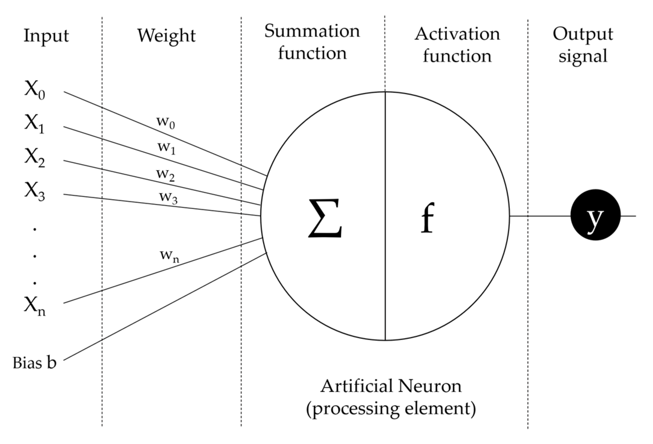
4.4. Neural Network Model
The initial dataset is divided into a training set (70%) and a test set (30%) to perform neural network modeling. The input layer comprises 31 units (excluding the bias unit), while the hidden layer contains 10. The hyperbolic tangent activation function was used for the hidden layer, while the Sigmoid function was used for the output layer, with the sum of squares used as the error function. Batch was used as a type of training, with maximum training epochs computed automatically. The model’s performance is evaluated using classification metrics on both the training and testing datasets (
Table 8).
The model demonstrated an overall accuracy of 76.8% on these training data, indicating that it effectively learned the patterns in these data. The overall accuracy of these testing data was 76.6%, slightly lower than the accuracy of these training data. This suggests the model generalizes well to unseen data and does not suffer from overfitting. Sensitivity, with 85.0% for the training set and 83.6% for the testing set, reflects the model’s strong performance in detecting instances of speeding. Specificity was comparatively lower, at 65.6% for the training set and 67.1% for the testing set. A model with two hidden layers was created for control, but the performance was not better than the initial one-hidden layer model. The factor that proved to be the most influential is the speed limit, followed by the distance to the closest intersection, roadway width, ASDT, and vehicle group.
The AUC for the neural network model was 0.840 for both training and testing datasets, indicating that the model has good discriminative ability (
Figure 2). An AUC of 0.840 means an 84% chance that the model will correctly distinguish between a randomly chosen positive instance (speeding) and a randomly chosen negative instance (no speeding). These results further support the effectiveness of the neural network model in predicting speeding.
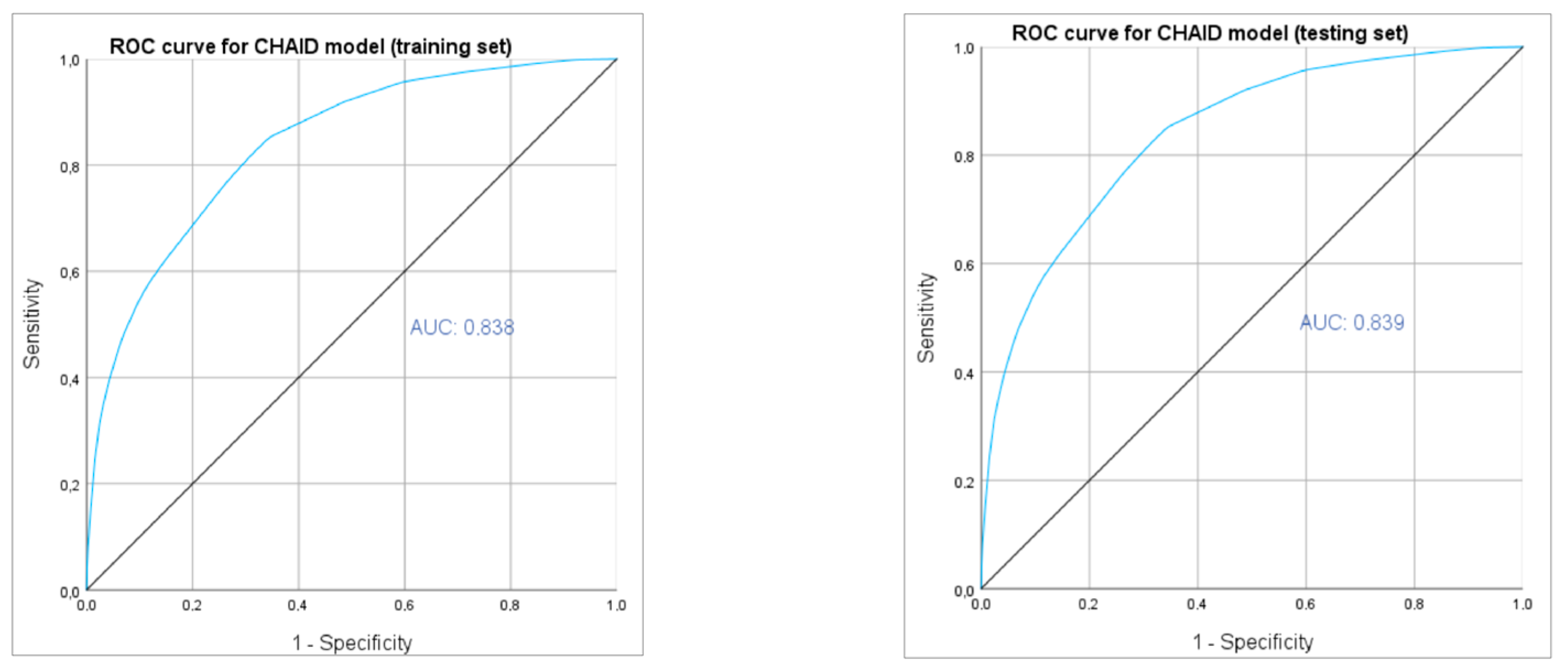
4.5. Chi-Squared Automatic Interaction Detector (CHAID)
The Chi-squared Automatic Interaction Detector (CHAID) model was employed to analyze factors influencing speeding behavior. The model, validated through a split sample approach (70% training set, 30% test set), identified six significant predictors of speeding: distance to the closest intersection, ASDT, vehicle group, time of the day, day of the week, and width across the roadway. With tree depths of 3 and 160 nodes, including 115 terminal nodes, the model provides detailed insights into how these factors influence speeding behaviors across different contexts.
The risk estimates for speeding obtained from the CHAID model are 0.231 and 0.232, with a standard error of 0.000 for both datasets. These estimates reflect the stability and consistency of the model’s predictions across training and test datasets. In classification results for speeding, the training dataset shows an overall correct prediction percentage of 76.9% (
Table 9). The sensitivity was high, with values of 85.2% for both the training and testing sets. This suggests that the model is robust in detecting speeding cases. The specificity was lower, with 65.5% on the training set and 65.3% on the testing set, indicating that the model has a moderate error rate in classifying non-speeding instances. These metrics indicate the model’s effectiveness in classifying instances of speeding based on the specified variables and the CHAID growing method.
The CHAID model demonstrates predictive solid performance, as evidenced by AUC values of 0.838 for the training set and 0.839 for the testing set (
Figure 3). These AUC values indicate that the model can discriminate between speeding and non-speeding cases, performing consistently well on both the training and testing datasets. The close similarity in AUC values suggests that the model generalizes effectively to new data, maintaining its accuracy and robustness outside the initial training environment.
4.6. Random Forest Model
The random forest model trained in this study is capable of predicting speeding behavior appropriately. Using a dataset of 3,236,697 observations (70% training set, 30% test set), the model comprising 500 trees achieved an out-of-bag (OOB) prediction error (Brier score) of 0.1597. On the training set, the model achieved an accuracy of 76.8% (95% CI: 76.74–76.83%), with a sensitivity of 84.4% and a specificity of 66.35%. On the test set, the model maintained a similar accuracy of 76.8% (95% CI: 76.73–76.87%), with a sensitivity of 84.5% and a specificity of 66.3%. The results are presented in
Table 10. These metrics demonstrate the model’s consistency and robustness across different datasets. Regarding predictors’ importance, the ones with the highest importance are speed limit, distance to the closest intersection, ASDT, and roadway width.
The random forest model demonstrated strong discriminative power, achieving an AUC of approximately 0.840 and 0.841 for the training and the testing dataset, respectively (
Figure 4). This high AUC indicates excellent performance in distinguishing between speeding and non-speeding instances.
5. Discussion
5.1. Average Values of Speeding Concerning Vehicle Groups
The classification of vehicles into five groups, based on length, was a pragmatic approach to ensure sufficient sample sizes of each group for meaningful analysis. This consolidation likely enhanced the robustness of subsequent statistical tests by mitigating the issue of minor vehicle frequency, which could lead to unreliable estimates and conclusions. Given that the specified groups of vehicles differ significantly in their driving-dynamic characteristics, the amounts of speeding for them were observed before analyzing the factors influencing speeding. Furthermore, the groups were compared with the basic assumption that the highest speeding was recorded among motorcyclists.
With a mean speeding amount of 24.11 km/h, motorcycles are the fastest vehicles, significantly surpassing other vehicle groups by more than 10 km/h. This result indicates a higher propensity for speeding among motorcyclists, highlighting them as a critical category. Further, as expected, passenger cars and vans showed similar speeding behavior, with mean speeds of 13.22 km/h and 13.15 km/h, respectively. Finally, cargo vehicles and buses exhibit the lowest speeding amounts, with means of 11.39 km/h and 10.03 km/h, respectively. This may reflect the professional nature of drivers in these categories or inherent vehicle characteristics that limit speed.
Earlier studies confirmed that motorcyclists are more likely to exceed the posted speed limit compared with passenger cars and other motor vehicles [
48,
49,
50,
51]. Furthermore, the results of this study are consistent with previous research, stating that motorcyclists are more likely to speed on rural roads due to motorcycle maneuverability and riders’ enjoying fast riding [
52]. Some studies point out that there is also a significant difference in speed between different types of motorcycles (e.g., sports and enduro), which can be an implication for future research [
50].
5.2. Speeding Prediction Models
This study applied several modeling techniques to examine the factors influencing speeding behavior and evaluate their predictive performance. The methods compared include binary logistic regression, neural network, CHAID classification tree, and random forest. Each model has distinct characteristics, strengths, and limitations, as discussed below.
All models showed a more accurate prediction of “Yes” cases, with a sensitivity greater than 84%. All approaches showed decent results when observing the models’ accuracy (>74%).
Table 11 compares the performance of four classification models across six key metrics: sensitivity, specificity, accuracy, precision, F1-Score, and Cohen’s Kappa. The binary logistic model exhibits the highest sensitivity at 89.30%, demonstrating strong performance in identifying true positive cases (e.g., identifying “Yes” instances); however, this is paired with the lowest specificity (55.00%), indicating weaker performance in correctly identifying true negative cases (e.g., identifying “No” instances). On the other hand, the machine learning models show a more balanced performance. Sensitivities for the neural network, CHAID tree, and random forest models hover around 85%, while specificities range from 65.41% to 66.14%. In terms of accuracy, all three machine learning models perform similarly, with the CHAID tree model achieving the highest accuracy at 76.85%, followed closely by the neural network (76.82%) and random forest (76.78%).
Precision and F1-Score further confirm the balanced performance of the machine learning models, with the random forest model showing the highest precision (77.31%) and the CHAID tree model achieving the best F1-Score (80.94%). Cohen’s Kappa values, which measure overall agreement between predicted and observed classifications, are also higher for the machine learning models, with the neural network model slightly outperforming the others (0.517), suggesting a better overall predictive quality compared with the binary logistic model (0.459).
Several aspects can explain the similar performance across the models. First, the data quality and structure likely offer transparent relationships between variables, making it easier for simpler models, such as logistic regression, to perform well. Moreover, the complexity of the problem may not demand highly sophisticated models, so machine learning methods such as neural networks or decision trees do not provide significantly better results. Furthermore, without extensive hyperparameter tuning, the more complex models may not fully exploit their potential, resulting in only marginally better performances than more straightforward approaches. Last, the large sample size and the absence of all potential causal parameters in the dataset can influence the models’ similar performance. A large dataset often provides enough information for different models to achieve stable and consistent predictions, reducing variability in performance. This can lead to even simpler models capturing essential patterns effectively. Additionally, while the models’ performance is satisfying, there is a potential for including some more causal factors. Above all, the similarity of results between training and test sets generally indicates a good model performance and generalizability. The abovementioned explains why the models display similar sensitivity, specificity, and overall accuracy levels.
The table reveals that while speed limit and distance to the closest intersection are consistently significant predictors across multiple models, the importance of other factors such as ASDT, roadway width, and time-related variables varies depending on the model used. These variations suggest that the choice of model should align with the specific needs of the analysis, whether prioritizing simplicity or a more comprehensive, multifactorial approach; therefore, it will be essential for the authorities to evaluate these models against their specific datasets to determine the most suitable one for implementation.
The association between speeding and several explanatory variables was constructed with several modeling approaches, which aligns with the previous research. Given that the performance of all models is similar, binary logistic regression is the basis for further discussion, showing strong sensitivity (89.30%). By utilizing binary logistic regression, the findings are interpretable (outputs in the form of odds ratios (Exp(B), previously shown in
Table 7), statistically sound, and actionable, contributing meaningfully to the understanding of speeding behavior and its underlying determinants.
Higher speed limits are significantly associated with lower odds of speeding. This implies that as speed limits increase, drivers are less likely to exceed them. This trend may be attributed to factors such as enforcement practices and adjustments in driver behavior. In addition, it might imply that drivers feel bored or too slow at lower speeds or even think that posted speed limits do not comply with the road design. The difference between the road design and the posted speed limit can also lead to speeding [
53]. Roadway characteristics substantially impact speed selection behavior, leading drivers who usually tend to drive fast to increase their speeds more than slower drivers when opportunities to drive faster are present [
54,
55]. Another study shows that drivers justify speeding by saying the speed limits are too low, the road conditions allow higher speed, or it is a habit [
56]. Kutela et al. concluded that the analysis of speed limits reveals an increase in the likelihood of speeding as the speed limits increase; however, the design difference should be taken into account [
24]. Similarly, Cai et al. (2021) confirmed that drivers are more likely to exceed the speed limit when the speed limit is low [
22]. Other studies also confirmed that speeding is more likely to occur on low-speed limit roads [
57], concluding that drivers choose their operating speed based on the other drivers’ speed [
58]; therefore, the speed distribution should serve as the foundation for determining suggested speed limits, with the final recommended value considering roadway type, context, safety performance, and other relevant characteristics [
59].
Research shows that a wider shoulder is associated with higher speeds, while narrower lanes encourage a speed reduction [
22]. Contrary to expectations, this study revealed that a wider roadway is associated with a lower likelihood of speeding; however, this must be considered cautiously since the difference between road width was relatively small (St. Dev. = 0.534 m). Interestingly, the roadside without a well-maintained shoulder and safety barrier is a more significant indicator of speeding than where the shoulder has a curb and/or a safety barrier. That may indicate that, in addition to the safety function, protective barriers and curbs impact the drivers’ perception, i.e., drivers are more careful not to hit the roadside object.
Similar to previous research, increased traffic can be connected to reduced speed [
60,
61]. The fact that the importance of variables such as distance to the closest intersection and ASDT has been shown indicates that traffic flow characteristics influence speed selection. In other words, the influence of other vehicles and increased driver’s caution when approaching or passing through an intersection is possible. This is consistent with previous studies showing that the least “smooth driving” is expected in urban areas (i.e., cities) [
62]. Since the increased share of speeding vehicles is expected outside urban areas, the selection of measurement locations in this research is justified when discussing factors potentially affecting speeding. Further, it can be expected that speeding will occur outside the settlements, even in rural areas, as well as on road sections where overtaking is allowed, which this study confirmed.
Weekends, notably Sundays, show increased odds of speeding, particularly in combination with nighttime and dawn driving, which is associated with a higher likelihood of speeding. The finding is particularly worrying since crashes, especially single-crashes, often occur during nighttime, at weekends, and under low traffic volume [
63]. On the other hand, some research shows that it is more likely that speeding will occur during evening and midday weekend hours [
64]. This difference may indicate that it is necessary to consider the geographical and cultural components when modeling speeding behavior or discussing transportation in general since the dynamics of people’s lives and habits can vary.
The analysis within our research indicated significant differences in speeding behavior across various vehicle groups. The results suggest motorcycle riders are more likely to be involved in speeding incidents than all other drivers. Specifically, as vehicle type changes from motorcycles to other groups, the likelihood of speeding decreases significantly. This expected result underscores the distinct driving behaviors and speed compliance levels associated with different vehicle types, highlighting motorcycles as a more prominent risk group for speeding-related incidents. Previous studies confirm motorcycle riders are more prone to speeding than other drivers [
52]. The above is particularly worrying considering that research shows that excessive speed significantly affects the occurrence of severe injuries and fatalities among motorcyclists [
65,
66].
While most of this study’s findings align with previous research, which confirms the role of factors such as speed limits in influencing speeding behavior, there were also some notable variations. These diverse indicators suggest that geographical and sociological aspects may play a significant role in shaping speeding tendencies. For example, the analysis revealed that temporal factors, such as the day of the week and time of day, significantly affect speeding likelihood. This indicates that drivers’ behavior might be influenced by social or cultural norms tied to specific times, such as weekend driving habits or night-time driving patterns. This variation could also indicate regional differences in driving culture, law enforcement practices, or public awareness of road safety, which more standardized driver behavior models might need to capture fully.
5.3. Limitations and Future Implications
This paper provides valuable insights into the factors influencing speeding behavior and choosing the appropriate modeling approach; however, several limitations should be acknowledged. This study did not account for individual driver characteristics such as age, gender, driving experience, or driving history. This means that only the vehicle and road characteristics were taken into account; however, this information can be unavailable to road authorities since they do not know the drivers’ characteristics when posting speed limits. Still, according to some researchers, driver attitude and other driver features strongly correlate with obeying speed limits [
67,
68]. The problem is solved to some extent by using groups of vehicles since a specific group of drivers is often associated with some typical behavior in the literature.
Further, the speed measurements were point-based, capturing speed at specific locations rather than over a continuous stretch of road. This method may not fully represent the overall driving behavior and could miss variations in speed between measurement points.
Finally, the dataset in this study represents summer measurements only. Although this ensures uniform measurement conditions, future research could include data from other seasons when conditions differ (e.g., snow, fog, etc.). On the other hand, favorable weather conditions are one of the prerequisites for free traffic flow, which is a vital assumption when inspecting speeding.
According to the presented results, the focus of future research could be more specific, for example, more detailed monitoring and data collection on motorcyclists’ movements (e.g., naturalistic data collection). Furthermore, it could be fruitful to separately observe weekends as a perilous period from the point of view of driving speed. Another potential approach is to observe speeding by class, based on the amount of speeding, and to observe cases inside and outside the settlement separately since the results show a higher possibility of speeding outside the inhabited settlement; however, the sample size presented in this study is one of its key advantages, enhancing the reliability and generalizability of the findings, as it reduces the likelihood of sampling bias and increases the precision of estimates. Furthermore, the sample size allows for detecting subtle relationships between the predictors and the likelihood of speeding and for a more granular analysis of subgroups, such as different vehicle types. In this context, the presented research is a base point for directing further examination, employing a more analytical approach.
Based on everything presented, there is a significant potential for further expansion of individual models so that they can ultimately be applied. By applying the results of those models, road authorities and law enforcement offices could precisely predict locations for the implementation of traffic calming measures or the installation of speed cameras. This can contribute to lower costs and increased traffic safety.
6. Conclusions
This study aimed to identify the key factors influencing speeding behavior on Croatian state roads using various statistical and machine-learning methods. By analyzing data collected from traffic counters on rural roads over two years, the research explored the impact of vehicle type, road characteristics, time of day, and other variables on speeding occurrences. Among the models, the random forest demonstrated superior performance, achieving an accuracy of 76.8% and a robust discriminative power, indicating its effectiveness in predicting speeding behavior; however, binary logistic regression could be one of the most useful models because of its favorable interpretability. The findings consistently highlighted the speed limit as the most significant predictor of speeding, with lower speed limits strongly associated with increased speeding likelihood. The distance to the closest intersection and the width of the roadway also emerged as influential factors. Vehicle type, time of day, and day of the week further contributed to speeding behavior, with motorcycles exhibiting the highest average speeding and speeding more likely to occur during nighttime and weekends.
This study uniquely contributes to road safety research by comprehensively analyzing speeding factors on rural roads in Croatia, a region underrepresented in previous studies. Combining traditional and advanced modeling techniques offers a more robust analytical approach and examines a distinctive set of factors, including some rarely explored in this context. These insights provide practical recommendations for targeted interventions, enhancing the understanding of speeding behavior in specific geographical and infrastructural settings. Overall, this research contributes valuable insights into the multifaceted factors influencing speeding behavior, thereby supporting the development of targeted interventions and policies aimed at enhancing road safety. Some general suggestions for road authorities can be provided:
Utilize Intelligent Transportation Systems (ITS): Implement advanced traffic management systems that leverage real-time data and analytics to optimize traffic flow and enhance enforcement measures, such as strategically placed speed cameras.
Focus on Eco-Friendly Road Design: Implement road-narrowing techniques at transition zones, such as residential areas and intersections, to effectively reduce vehicle speeds. By designing roadways that physically guide drivers to slow down, these measures enhance safety while also promoting eco-friendly practices through the use of sustainable materials and designs that minimize environmental impact.
Enhance Road Visibility and Safety: Improve the visibility and frequency of speed limit signs by incorporating digital displays that adapt to real-time conditions, ensuring drivers are consistently informed of speed regulations. Additionally, perceptual road markings should be utilized to create a visual narrowing effect, which can psychologically encourage drivers to reduce their speed. This combination of advanced signage and perceptual techniques not only enhances visibility but also significantly improves safety by promoting more cautious driving behavior in critical areas.
Data-Driven Speed Limit Adjustments: Regularly review and establish realistic speed limits based on comprehensive analyses of road types, traffic volumes, and crash histories, ensuring that limits are both safe and enforceable.
Tech-Enhanced Educational Campaigns: Initiate campaigns that leverage digital platforms to inform drivers about the significance of adhering to speed limits and the dangers linked to speeding, thereby promoting a culture of safety on the roads.
Further, based on the results presented in this study, some more specific and applicable suggestions for road authorities, policymakers, and law enforcement can be proposed:
Speed Limit Review: Conduct a thorough revision of posted speed limits by analyzing operational speeds at critical locations, assessing the current condition of the infrastructure, and considering additional contextual factors such as land use, pedestrian activity, and road geometry. This approach helps ensure that speed limits are appropriate for the environment and encourages safer driving behavior.
Road Safety Equipment Installation: Strategically install appropriate road safety equipment, such as crash barriers and guardrails, in high-risk areas to reduce the severity of crashes. These physical measures not only protect drivers but also act as visual cues, encouraging speed reduction and caution in known crash-prone zones.
Increased Police Presence: Implement more frequent and targeted police patrols, especially during high-risk periods such as weekends and holidays when speeding and dangerous driving behaviors are more prevalent. A visible law enforcement presence is a deterrent to speeding and reckless driving.
Improved Intersection Marking: Ensure consistent and timely installation of highly visible and uniformed road markings at intersections to warn drivers clearly. This can significantly enhance driver awareness and reduce the likelihood of speeding in these complex traffic zones, minimizing potential collisions.
Motorcycle Safety Focus: Pay special attention to areas with high motorcycle traffic by identifying potential hazards and launching targeted safety campaigns. Educate motorcyclists and other road users about safe practices and implement infrastructure improvements to enhance motorcycle safety.
Traffic Surveillance Enhancement: Install traffic monitoring cameras at locations where errant drivers, particularly motorcyclists, are frequently observed. These cameras help enforce traffic laws in cases where it is challenging for police to apprehend offenders, such as motorcyclists fleeing from officers or concealing license plates.
Crash and Speeding Monitoring: Continuously track and analyze data related to traffic crashes caused by speeding, including the severity of injuries and fatalities. This ongoing evaluation can inform future road safety measures and adjustments to enforcement strategies, helping to reduce the incidence of speed-related crashes over time.
Implementing measures that address the identified factors, such as integrating advanced road design improvements and stricter enforcement of speed limits, can significantly reduce speeding incidents and associated risks. Through a comprehensive approach that combines enforcement, innovative design, and technology, we can create safer road environments that minimize the dangers of speeding.


