Article

Developing Statistical and Multilayer Perceptron Neural Network Models for a Concrete Dam Dynamic Behaviour Interpretation †

by
Andrés Mauricio Guzmán Sejas
1,*,
Sérgio Pereira
1,2,
Juan Mata
3 and
Álvaro Cunha
1,2
1
Faculty of Engineering of the University of Porto (FEUP), Rua Dr. Robert Frias, 4200-465 Porto, Portugal
2
Construct-ViBest, Rua Dr. Robert Frias, 4200-465 Porto, Portugal
3
National Laboratory for Civil Engineering (LNEC), Concrete Dams Department, Av. do Brasil 101, 1700-066 Lisbon, Portugal
*
Author to whom correspondence should be addressed.
This paper is an extended version of the work “Dynamic Behaviour of a Concrete Dam: Development of Statistical and Machine Learning Models for Interpretation of Monitoring Data”, which won the Best Academic-Scientific Paper award at the Fifth International Dam World Conference in Lisbon, Portugal.
Infrastructures 2025, 10(11), 301; https://doi.org/10.3390/infrastructures10110301
Submission received: 18 September 2025 / Revised: 17 October 2025 / Accepted: 30 October 2025 / Published: 9 November 2025
(This article belongs to the Special Issue Preserving Life Through Dams)

Abstract

This work focuses on the dynamic monitoring behaviour of concrete dams, with a specific emphasis on the Baixo Sabor dam as a case study. The main objective of the dynamic monitoring is to continuously observe the dam’s behaviour, ensuring it remains within expected patterns and issuing alerts if deviations occur. The monitoring process relies on on-site instruments and behaviour models that use pattern recognition, thereby avoiding explicit dependence on mechanical principles. The undertaken work aimed to develop, calibrate, and compare statistical and machine learning models to aid in interpreting the observed dynamic behaviour of a concrete dam. The methodology included several key steps: operational modal analysis of acceleration time series, characterisation of the temporal evolution of observed magnitudes and influential environmental and operational variables, construction and calibration of predictive models using both statistical and machine learning methods, and the comparison of their effectiveness. Both Multiple Linear Regression (MLR) and Multilayer Perceptron Neural Network (MLP-NN) models were developed and tested. This work emphasised the development of several MLP-NN architectures. MLP-NN models with one and two hidden layers, and with one or more outputs in the output layer, were performed. The aim of this work is to assess the performance of MLP-NN models with different numbers of units in the output layer, in order to understand the advantages and disadvantages of having multiple models that characterise the observed behaviour of a single quantity or a single MLP-NN model that simultaneously learns and characterises the observed behaviour for multiple quantities. The results showed that while both MLR and MLP-NN models effectively captured and predicted the dam’s behaviour, the neural network slightly outperformed the regression model in prediction accuracy. However, the linear regression model is easier to interpret. In conclusion, both methods of linear regression and neural network models are suitable for the analysis and interpretation of monitored dynamic behaviour, but there are advantages in adopting a single model that considers all quantities simultaneously. For large-scale projects like the Baixo Sabor dam, Multilayer Perceptron Neural Networks offer significant advantages in handling intricate data relationships, thus providing better insights into the dam’s dynamic behaviour.

1. Introduction

A dam failure represents a catastrophic event, typically involving a breach followed by a flood wave, which may result in significant loss of life and property. Even in cases where the reservoir’s availability or the reliability of its operation is merely impaired, essential economic interests may be disrupted, and environmental damage may occur. For these reasons, dam owners and engineers have consistently placed dam safety as a paramount concern [1].
Dam failure is generally a complex process, usually initiated by an undetected abnormality. Progressive deterioration, often unnoticed, may then lead to further damage and ultimately to disaster. This highlights the critical role of systematic inspection and monitoring of dams, together with timely data analysis and interpretation.
The primary tasks of dam monitoring include instrument measurements; data verification; data processing and analysis; and the interpretation and reporting of results. The central objective of monitoring is to generate reliable information for assessing the dam’s continued performance and safety. During operation, monitoring involves two complementary aspects: short-term and long-term monitoring.
Short-term monitoring focuses on detecting rapid anomalies in dam or reservoir behaviour that may compromise safety or operability, requiring immediate intervention (e.g., restrictions to operation, repairs, or, in extreme cases, warnings). Long-term monitoring, in turn, aims at identifying gradual changes in condition and behaviour, facilitating comprehensive safety assessments (including the validation of design parameters) and supporting maintenance planning.
Both functions are equally important. Although short-term monitoring is often viewed as sufficient, understanding long-term behaviour is frequently essential for explaining anomalies detected by critical instruments. Moreover, gradual trends can be as significant for safety as abrupt changes. These two functions are therefore interdependent, operating on different temporal scales of data analysis [2].
The use of soft computing and machine learning techniques, such as fuzzy logic and neural networks, in dam engineering began to gain popularity in the late 1990s and early 2000s. The first application of these techniques for modelling dam behaviour is arguably the work by Bossoney [3], closely followed by Hattingh L.C. [4]. The main purpose was to overcome the limitations of the traditional Hydrostatic–Season–Time (HST) model [5] in identifying nonlinear behaviour and accounting for complex phenomena. This remains the main application of soft computing in dam engineering to date, facilitated by the development of new algorithms and the increase in available monitoring data resulting from the installation of automatic data acquisition systems (ADAS) [6].
According to Bourdarot et al. [7], modelling calibration and validation is a classical step under static conditions, based on monitoring results. Hydrostatic, thermal, and irreversible effects are mainly considered. Under dynamic conditions, however, calibration remains rarer and more complex. While calibration with monitoring data can provide an evaluation of quasi-static properties, estimating dynamic characteristics requires assumptions regarding dynamic effects [8].
Monitoring the dynamic behaviour of concrete arch dams is increasingly viewed as an essential component of safety control procedures. Characterising the dynamic response is particularly important for structures located in seismic regions [9]. Lessons learned from the CFBR–JCOLD cooperation on concrete dams have shown that natural frequencies vary with water level and seasonal temperatures, and that this variation can be of the same order of magnitude as frequency variations caused by damage [7]. Consequently, it is necessary to use regression models to predict the normal evolution of natural frequencies. The study also identified that natural frequency [7] (i) decreases when the reservoir water level rises due to the increase in added mass and (ii) decreases in winter due to joint opening. This has been confirmed by observations of the natural frequencies of adjacent cantilevers with different heights, which converge in summer but diverge in winter.
The evolution of dynamic characteristics may also help to detect the initiation or development of damage phenomena throughout the structure’s lifetime [9].
In recent years, several studies have explored the application of advanced deep learning models and statistical analyses to monitor and predict dam safety behaviour, focusing particularly on displacements [10,11,12,13,14], joint movements [15], and seepage [16]. However, only a limited number of studies have addressed dynamic behaviour monitoring results.
Several articles propose and validate neural network architectures, such as autoencoders [17], LSTM [18,19,20], and DenseNet–LSTM [21], highlighting their superior accuracy in predicting deformations compared to more traditional statistical and machine learning models. Some studies also address the integration of spatial information to improve prediction accuracy at adjacent monitoring points [22]. Another area of research tackles the challenge of insufficient observation data for older or newer dams through transfer learning frameworks [23].
The adoption of machine learning and deep learning models for analysing dynamic behaviour, particularly for interpreting the evolution of natural frequencies monitored in dams during operation, remains scarce.
The authors aim to contribute to the expansion of scientific knowledge in characterising dynamic behaviour using machine learning models. In addition to improving the characterisation of natural frequencies according to the main loads, this work introduces a new perspective on the application of Multilayer Perceptron Neural Networks. Instead of analysing one natural frequency at a time, this study proposes a model that represents the global dynamic behaviour by simultaneously considering multiple natural frequencies.
In this work, after the introduction of the HST and the HTT (hydrostatic, temperature, time) approaches, a summary of the most used data-based models is presented, taking another step in its application to the analysis of data from the dynamic observation of large concrete dams. The Baixo Sabor dam was adopted as a case study, and the pattern behaviour of the natural frequencies, tracked from 2015 to 2018, was represented through both MLR and MLP-NN models. Finally, a brief discussion about the good performance of models is presented.

2. Materials and Methods

2.1. Interpretation of Structural Behaviour Based on HST and HTT Approaches

In the normal operation phase of the dam’s life, the thermal effect is directly related to the air and water temperature variations. There are two main approaches for choosing the parameters that represent the thermal effect in data-based models [24]: the HST approach and the HTT approach. The HST approach is the most common for developing quick models in the field of dam engineering, being the approach adopted in this work. This approach is based on the hypothesis that the variable under study, such as horizontal displacements, depends on a combination of hydrostatic load effects, seasonal temperature variations represented in a simplified manner through the sum of sinusoidal functions with an annual period, and the effect of time [5,24].
This approach is only applicable if there is a sufficient number of observations and the generated functions can model the pattern of the variable under study. The approach aims to approximate effects associated with a limited period at a specific point using Equation (1):
Y h i , S i , t i = U h h i + U θ θ i + U t t i + k + ε i
where
  • Y h i , S i , t i —The observed value of the variable under analysis in observation i , which depends on hydrostatic pressure, temperature, and the point in time when the observation is made;
  • U h h i ,   U θ θ i ,   U t t i —Components of the variable that correspond to the elastic effect of the reservoir water level, the elastic effect of seasonal temperature variations, and the effect of time in the i t h observation;
  • k —A constant that corresponds to the difference between observed and calculated values at the beginning of the calibration period;
  • ε i —The residual of the i t h observation, given by the difference between the estimated value and the observed value.
The effect of the water level can be represented by a polynomial function. The approximation can be made using the following Equation (2):
U h h =   a 1 h 4 +   a 2 h 3 +   a 3 h 2 + a 4 h
where h is the reservoir water height and a 1 ,   a 2 ,   a 3 ,   a 4 are the coefficients to be adjusted.
The temperature effects are related to variations in air and reservoir water temperatures and their influence on the thermal field of the structure. In the HST approach, the effect of temperature change can be considered as a proportional attenuation of air temperature changes, with a phase shift that depends on the depth along the analysed section. Straightforward data-based models typically do not use temperature measurements, as it is assumed that the thermal effect U θ can be represented by a sum of sinusoidal functions with a one year period. Thus, the effect of temperature variations is defined by a linear combination of sinusoidal functions, depending only on the day of the year [25], and can be represented as follows:
U θ d a n n u a l = b 1 cos d + b 2 sin d
with
d = 2 π t d 365               1 t d 365
where t d represents the number of days elapsed from the start of the year to the date of observation and b 1 ,   b 2 are the coefficients to adjust.
The effect of time on the structure is an irreversible component associated with the effects of inelastic actions, such as creep and/or concrete stress relaxation, as well as phenomena related to deterioration (e.g., concrete swelling).
The combination of polynomial functions is often used in the context of this component, with several ways to write Equation (5), depending on the author and the phenomena under study.
U t t = c 1 t 3 + c 2 t 2 + c 3 t + c 4 l n ( 1 + t a )
where t represents the number of days between the observation campaign and the beginning of the monitoring; a represents the number of days between the first filling and the date of the beginning of the analysis; and c 1 , c 2 , c 3 , c 4 are the coefficients to be adjusted.
Based on the HTT (Hydrostatic, Temperature, Time) approach, the model represents the thermal effect through information recorded in thermometers, which can be embedded in the concrete dam body. Better performance based on the HTT models approach than in HST models is usually expected. However, additional data (temperatures measured in the dam body) is required to perform HTT models. In this study, as mentioned earlier, the focus was on analysing the performance of the HST models.

2.2. The Multiple Linear Regression Model

The primary goal of Multiple Linear Regression (MLR) models is to predict response values (dependent variable) based on a set of predictor data (independent variables). A model can be built initially to understand the relationship between predictors and a dependent variable, and then once this relationship has been established, it can be used to produce predictions of the dependent variable based on known independent variables [26].
In the context of dam monitoring, certain loads trigger responses from the reservoir–dam–foundation system. The set of actions that stand out results from variations in environmental and operational conditions, such as the water level in the reservoir, temperature, and others.
If it can be confirmed that (i) there were no significant structural changes during the period under analysis; and (ii) the structure operates with low stress levels, displaying elastic, linear, and reversible behaviour, then the principle of superposition can be considered valid. This allows for simplification in analysis by using models built with the Multiple Linear Regression method.

2.3. The Multilayer Perceptron Neural Network Model

A Multilayer Perceptron Neural Network model (MLP-NN) is a type of feedforward neural network in which all nodes are interconnected across different layers. The concept of the perceptron, which is a supervised learning algorithm that includes node values, activation functions, inputs, and weights to compute outputs, is also a fundamental unit of an artificial neural network [27]. Figure 1 illustrates a generic example of a Multilayer Perceptron Neural Network, with an input layer having N input parameters, one hidden layer, L 1 , with Q processing elements, and an output layer, L , with M outputs.
The parameters have the following meaning:
  • x i p — input network i , from pattern p ;
  • P —number of patterns;
  • L —output layer;
  • L 1 —hidden layer;
  • N—number of inputs in input layer;
  • Q —number of processing elements in the hidden layer;
  • M —number of processing elements in the output layer;
  • w i j L 1 —synoptic weight between input network i from layer L 1 at processing element j;
  • s j L 1 , p —activation value at processing element j from layer L 1 , from pattern p ;
  • f j L 1 —activation function at processing element j from layer L 1 ;
  • y i L 1 , p —output unit i, from layer L 1 , from pattern p .
The set of patterns can be written as follows:
= x 1 1 , , x i 1 , , x N 1 , d 1 1 , , d k 1 , , d M 1 , , x 1 p , , x i p , , x N p , d 1 p , , d k p , , d M p , , x 1 P , , x i P , , x N P , d 1 P , , d k P , , d M P
where d k p is the desired target at processing element k, from pattern p .
The MLP-NN model operates only in the forward direction, meaning that each node passes its value to the next node in the forward direction only. The backpropagation algorithm is used to enhance the training model’s accuracy by adjusting the weights based on the error between the predicted and actual outputs. Each node in the input layer represents a distinct feature of the input data. The hidden layers are where the network performs its computations and learns to transform the input data. The complexity of the relationships in the input data influences the number of hidden layers required. In some models, a single hidden layer might be enough, whereas more complex models may require multiple hidden layers to effectively capture patterns in the data. Finally, the output layer provides the final prediction or classification [27]. The output value at the processing element k , in layer L 1 , y k L 1 , p , can be expressed as follows:
y k L 1 , p = f j L 1 , p s j L 1 , p
where the activation value, s j L 1 , p , was defined as
s j L 1 , p = i = 1 N y i L 1 , p · w i j L 1
For the hidden layer, the adopted activation function was the hyperbolic tangent. For the output layer, linear functions were adopted. The learning rule consists of the application of an optimisation process of updating the weights in form to minimise the error of a cost function. The cost function considered, C , was defined by the mean square error, as shown in (8).
C = 1 P p = 1 P 1 2 k = 1 M y k L , p · d k p 2
The updating of the weights, in each iteration, was carried out for the output layer as shown in (9) and for the hidden layer as shown in (10).
Δ w i j L = η g i j L = η p = 1 P d j p y j p f s j L , p y i L 1 , p
Δ w i j L 1 = η p = 1 P k = 1 M y k p d k p f k L s k L , p w j k L f s j L 1 , p y i L 1 , p
A single hidden layer with enough neurons can approximate any continuous function, making it powerful for a wide range of problems. An MLP-NN with two hidden layers can represent more complex functions with fewer neurons compared to a single-layer network. However, given the characteristics of the structural health monitoring problems related to the prediction of observed behaviour, the option for neural networks with one or two hidden layers is valid/plausible, and no major differences in performance are expected between these two types of networks.
In this work, the authors would like to present the differences and advantages of adopting neural networks with one or multiple outputs in the output layer. The MLP-NN models with multiple outputs in the output layer have the advantage of predicting multiple targets simultaneously, learning from the patterns in the output feature set. Therefore, there is some consistent prediction of the multiple outputs, representing the pattern of the observed behaviour, avoiding the need to train separate networks for each output. In turn, MLP-NN models with a single output in the output layer have the advantage of being simpler and easier to interpret because they directly map each input to one specific prediction.
Figure 2 shows the perfect example of the different architectures that can be used. In addition, it is also easier to trace how input features influence the single prediction, for the comparison of the performance of the models. The performances of the MLP-NN and MLR models are presented through the coefficient of determination, R 2 , and the standard deviation of the residuals, σ .

3. Case Study

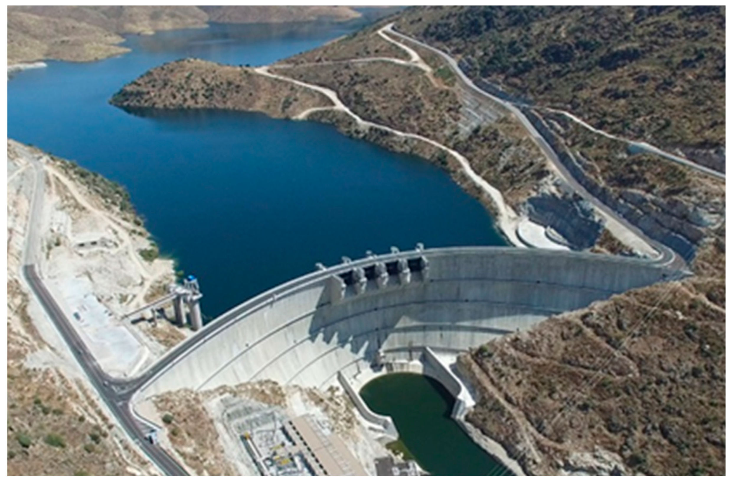
The Baixo Sabor dam is an important hydroelectric infrastructure located in the Sabor River in north-eastern Portugal. This dam is part of a larger project aimed at harnessing the hydroelectric resources in the region. It is situated in the district of Bragança, within the region of Trás-os-Montes and Alto Douro, known for its mountainous landscapes and rivers. The Sabor River is one of the main tributaries of the Douro River.
The dam construction began in 2008, with the first filling taking effect in 2015. It is a concrete double-curvature arch dam, embedded in a narrow valley zone. The dam is 123 m high at its crest, with a width of 6 m and 505 m long. The dam body has 32 blocks, separated by vertical contraction joints, which are crossed by six horizontal visiting galleries and one main drainage gallery. Figure 3 shows an aerial view of the representation of the dam [28].
The dynamic monitoring system installed in the dam is divided into three subsystems connected by optical fibre, with 12 uniaxial force balance accelerometers at the top, and 8 more positioned in the second and third visiting galleries [28]. The position of the 20 accelerometers is characterised and shown in Figure 4.
The dynamic monitoring system is configured to continuously record acceleration time series with a sampling rate of 50 Hz and a duration of 30 min at all instrumented points, thus producing 48 groups of time series per day.
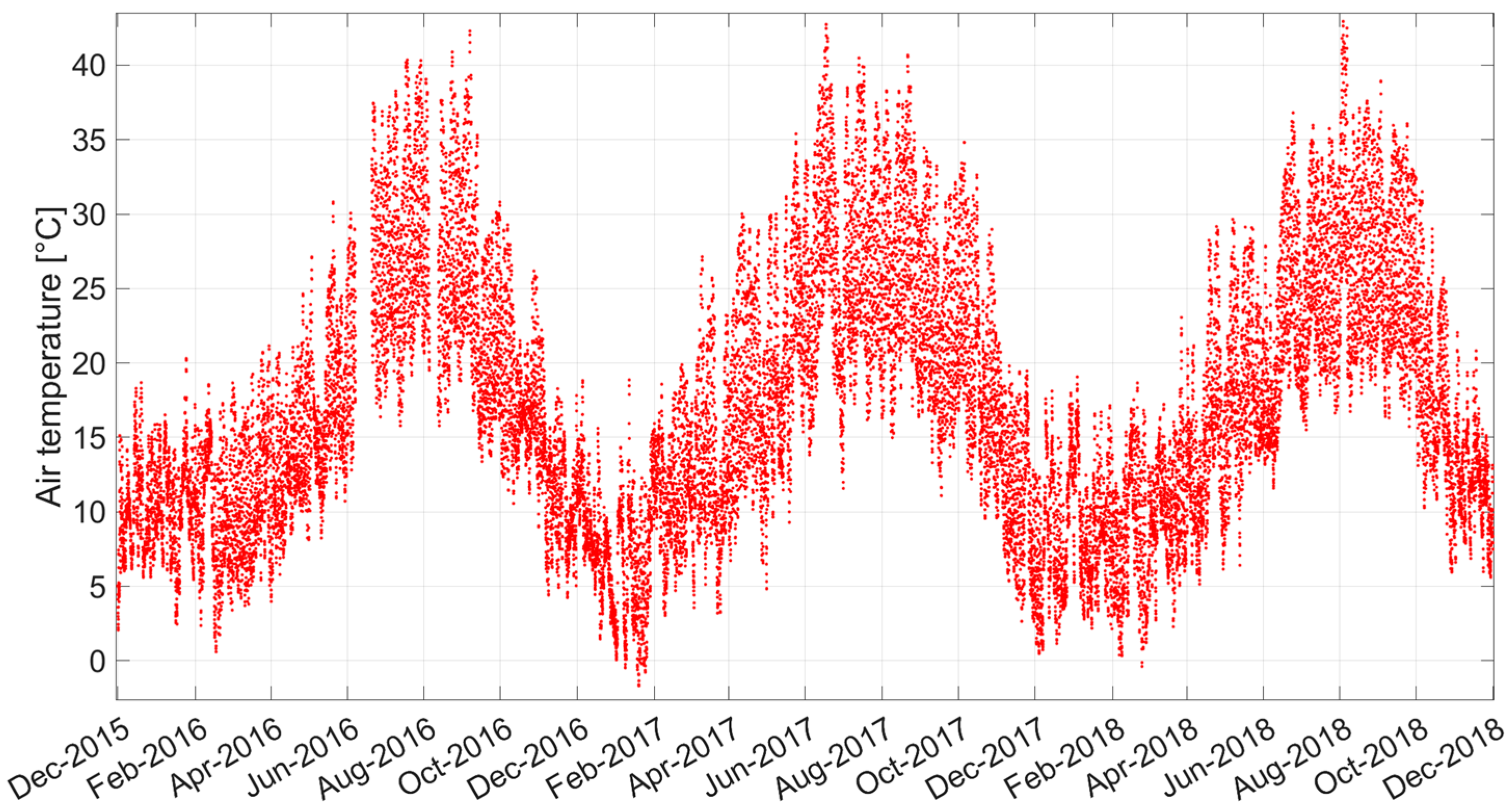
Figure 5 displays the air temperature recorded during a three-year monitoring period. The variations in temperature over time offer valuable information about the seasonal variations and climatic conditions in the region. Analysing these patterns can help in assessing the impact of air temperature on various aspects of the dam’s pattern behaviour.
In turn, Figure 6 illustrates the water level variation observed over a period of three years, including the last stage of the dam’s first filling. The data reveals variations in the water level over time due to the season, with more water in the reservoir during the spring and early summer and less during the autumn and early winter, and these fluctuations show almost the same behaviour over time, providing insights into the dynamics of the reservoir.
Seasonal variations affect the mass of the dam–foundation–reservoir system, as well as the stiffness of the concrete arch, therefore leading to fluctuations in the values of modal properties, making it essential to consider these environmental factors when assessing the structural dynamic behaviour of the dam over time.
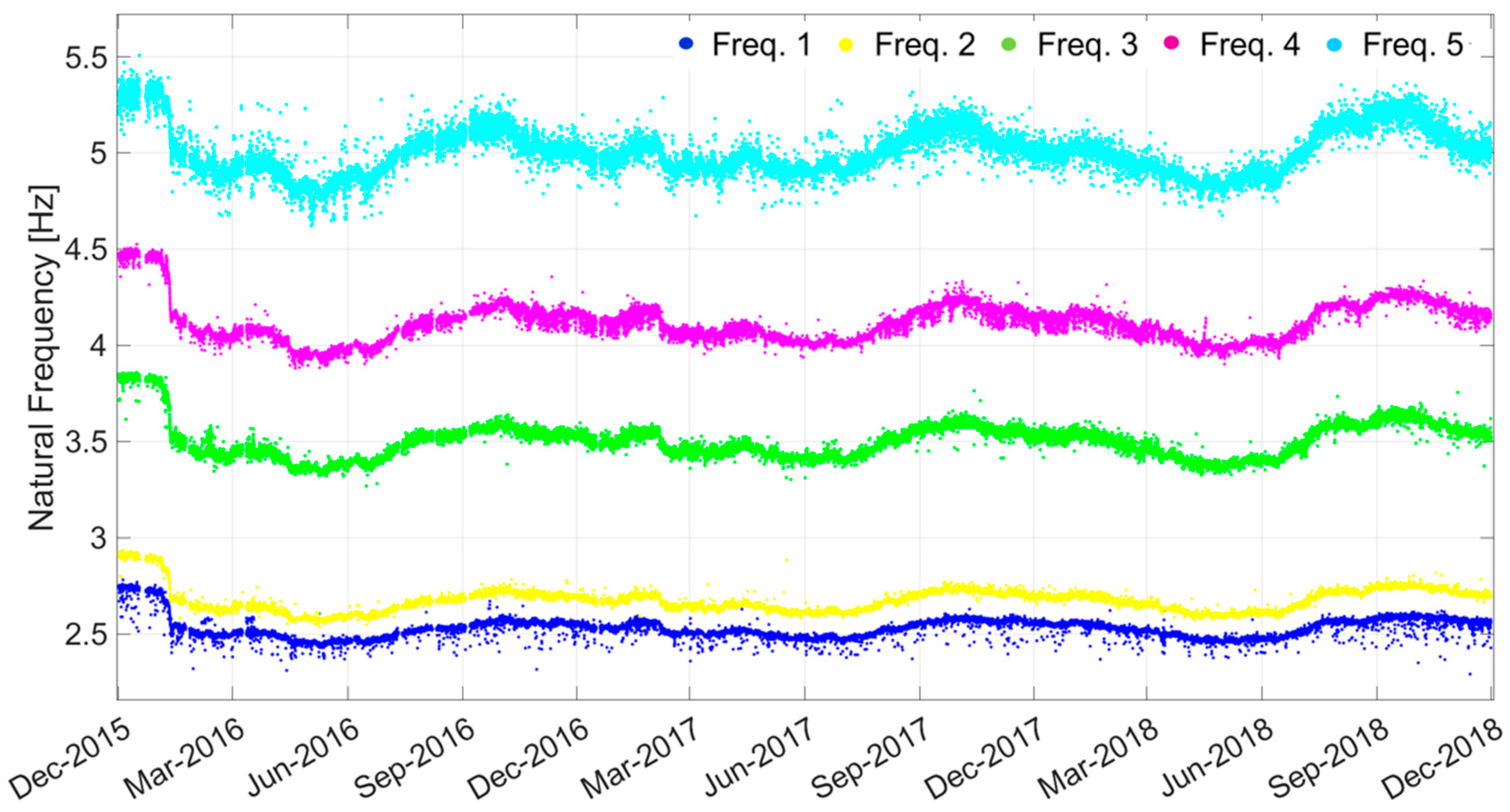
The continuous dynamic monitoring aims to identify and track the evolution of the dam’s dynamic characteristics under various operational and environmental conditions. Figure 7 illustrates the evolution of the natural frequencies obtained through continuous monitoring spanning three years. The dataset used for this research includes data monitored from 1 December 2015 (1/12/2015) at 00:00 hhours until 30 November 2018 (30/11/2018) at 23:00 h.
This extensive dataset allowed for the development of robust data-driven models to analyse the dam’s behaviour under various conditions. The continuous monitoring provided a detailed temporal resolution, facilitating the understanding of how the natural frequencies evolved over time.
The first mode’s natural frequency ranges from approximately 2.2 to 2.8 Hz, and the first five modes can be found below 5.5 Hz.
The sudden fall of natural frequency values in January 2016 is explained by the variation in the reservoir water level. Comparing Figure 6 and Figure 7, it is possible to notice that an inverse proportionality occurs between natural frequency values and reservoir water level. The natural frequencies of the structure decrease considerably and continuously during the first filling of the reservoir. This phenomenon is even clearer in January 2016, due to a sudden rise in the reservoir water level and a sudden drop in the frequency values, which would be expected given that a large amount of mass was added to the dam–foundation–reservoir system [28].

4. Results and Discussion

4.1. Multiple Linear Regression Models for the Characterisation of the Natural Frequency Pattern

The HST approach has primarily been used to analyse quasi-static physical quantities, such as horizontal displacements measured using the pendulum method. One of the recent innovations in this approach is the general characterisation of the natural frequency pattern through data-based models, which allows for the transposition of the HST approach in order to characterise the dynamic behaviour [25].
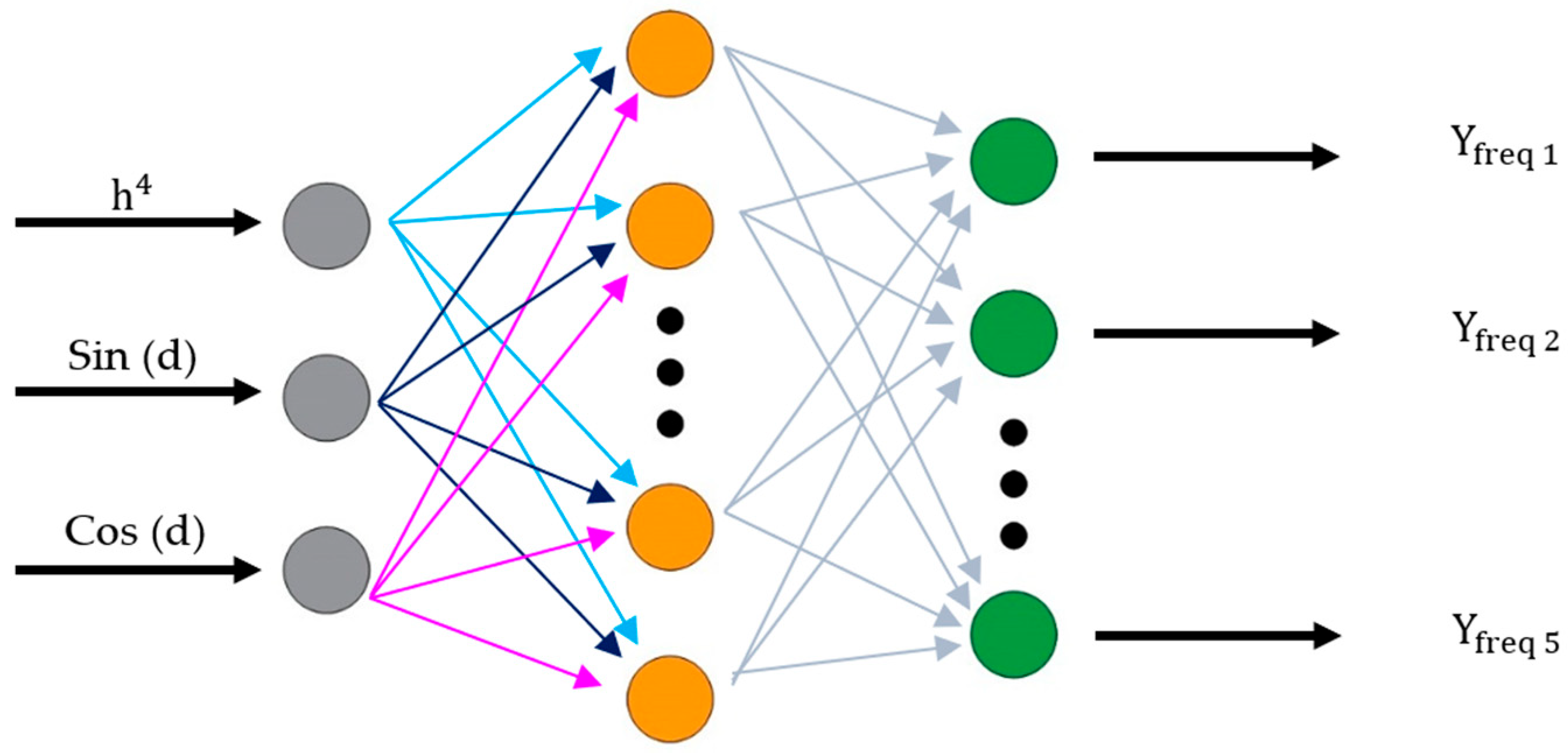
For the development of this research, the first term of the full polynomial ( h 4 ) is considered, which represents the water level in the reservoir and is mentioned in Equation (2). In addition, in the case of the sinusoidal thermal effect, the use of a variable representing the day of the year will be used as the argument for sine and cosine functions within a period of one year.
The main terms of the model adopted in this work are presented in Equation (11):
Y H S T = β 0 + β 1 h 4 + β 2 sin d + β 3 cos d
The natural frequencies estimated during the three years of continuous monitoring were used. Data from the first two years of monitoring, from 1 December 2015 (1/12/2015) to 30 November 2017 (30/11/2017), was used to train and to establish the base model. Furthermore, the remaining data, which refers to the third year of monitoring, from 1 December 2017 (1/12/2017) to 30 November 2018 (30/11/2018), were used to validate the quality of the forecasts provided by the regression model. Table 1 shows the results obtained from the training model based on the HST approach for the first five vibration modes. Table 1 allows us to identify the regression coefficients, which were used to conduct testing in the third year.
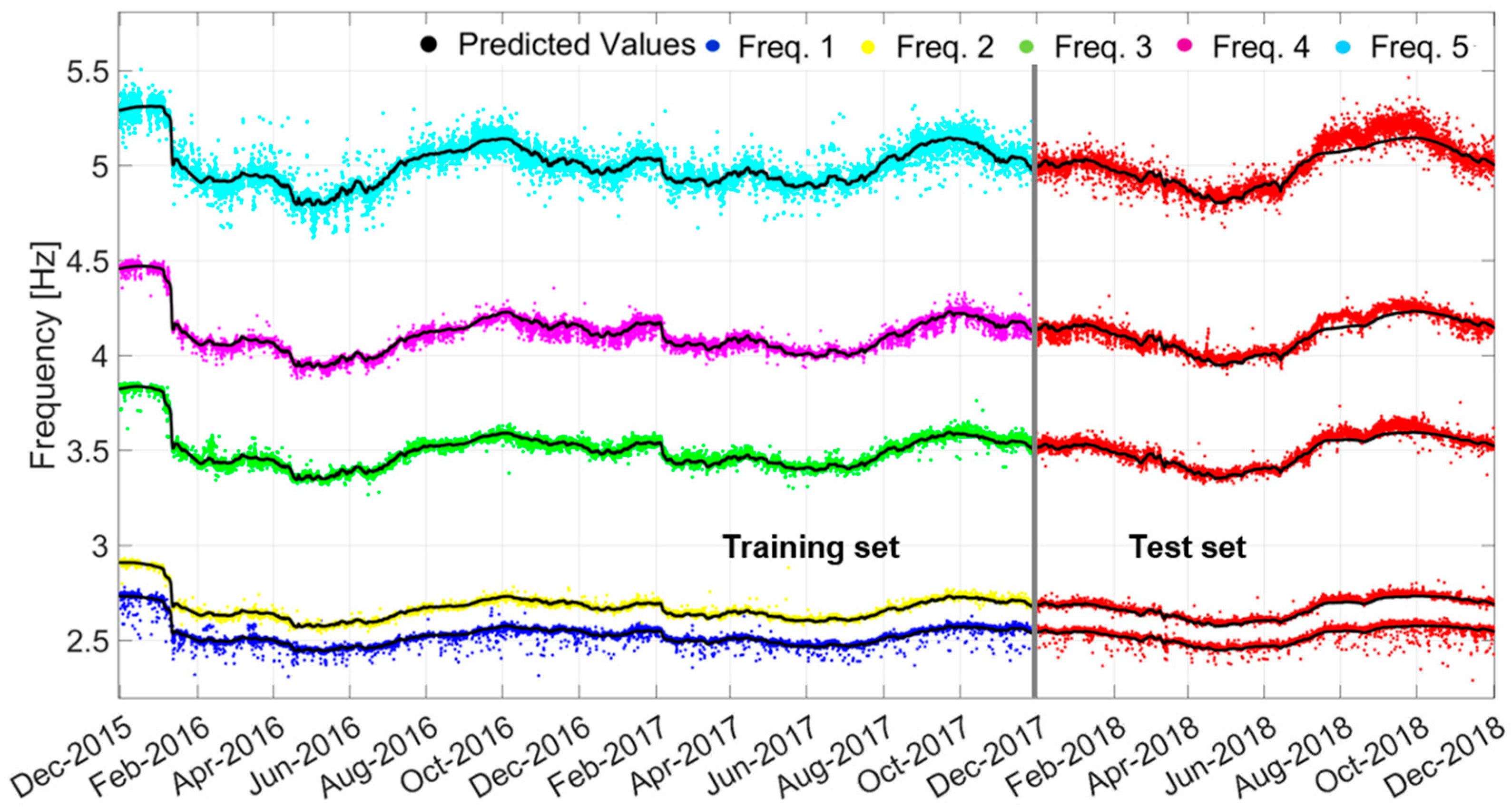
The predictions obtained from the MLR models for the training and for the test set are shown in Figure 8 to verify the quality of the models obtained. The performance parameters are presented in Table 2.
The performance parameters obtained were satisfactory, with a small decrease in the coefficients of determination compared to the training and testing set for all five vibration modes. Figure 8 also illustrates the prediction made, which exhibits smooth behaviour aligned with the actual values.

4.2. Multilayer Perceptron Neural Network Models

As referred to before, an MLP-NN model was also adopted. The same dataset as the regression model was used. In addition, an example of the architecture of these models based on neural networks with one output in the output layer is detailed in Figure 9. The same independent variables were considered as in the development of the Multiple Linear Regression model.
Using MATLAB software R2022a the fitrnet [29] function was employed for training and testing the model. The model presented was determined after an iterative process that considered two hidden layers, with a range of 1 to 15 neurons per hidden layer.
In the adopted architecture, the weights are important parameters that determine the strength and direction of the influence that one neuron has on another in the neural network; the inclusion of hidden layers in the neural network allowed the model to learn more abstract and complex representations of the data. In this specific case, different configurations of hidden layers were tested, with the purpose of identifying the structure that best captured the nonlinear relationships present in the data, resulting in a greater ability of the model to generalise and make accurate predictions.
The predictions obtained from the MLP-NN models for the training and for the test set are shown in Figure 10, which allows us to verify the quality of the models obtained. The performance parameters are presented in Table 3.
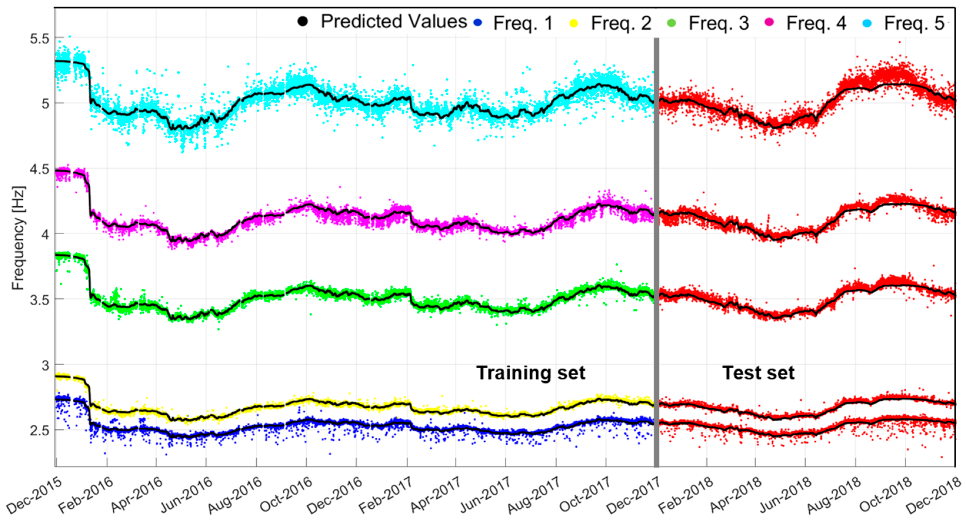
It is noteworthy that Figure 10 shows the result of a more adaptable and flexible behaviour of the MLP-NN models when compared to the MLR model, whose results are presented in Figure 8. An indication of this is the determination coefficient, which is higher for the MLP-NN model compared to the MLR models. Similarly, the analysis of the remaining variables shows that MLP-NN performs more effectively; however, the use of MLR remains valid, as its results are also very acceptable.
An MLP-NN with five simultaneous outputs in the output layer were considered, with each of the five outputs corresponding to the values of a natural frequency, as illustrated in Figure 11. The MLP-NN learning process was similar to that of the neural network described above, except that in this case each of the outputs was normalised between 0 and 1 to avoid biases resulting from frequencies having different magnitudes. In this case, the cost function to be minimised results from the sum of the squares of the residuals of the various outputs. The main results can be seen in Figure 12 and Table 4.

5. Conclusions and Final Remarks

The developed work aimed to perform monitoring and assessment of the dynamic behaviour of a concrete dam through MLR and MLP-NN models by tracking the evolution of its dynamic behaviour, ensuring that it stays within expected variations. This activity relies on observation through on-site instrumentation and behaviour models.
Both MLR and MLP-NN methods fulfilled their function of capturing and predicting information for an unseen season, with both models considered functional based on performance, although selecting an appropriate method can be complex and dependent on various factors.
For the Baixo Sabor dam case study, the following considerations can be made regarding which criterion or model is necessary:
  • Overall performance: Both methods performed well in predicting data, suggesting that both approaches are suitable for the problem at hand.
  • Prediction accuracy: The neural network models slightly outperformed the regression model in terms of prediction accuracy. This suggests that the neural network was better able to capture the relationship between input features and the target variable compared to the regression model.
  • Model flexibility: The neural network models can capture complex relationships between input features and the target variable, explaining its better performance on a dataset.
  • A neural network with multiple outputs offers the advantage of capturing relationships among different target variables within a single model. This approach can reduce training time and help maintain consistency in predictions, especially when the outputs are correlated and sufficient data is available for all targets. However, networks with multiple outputs can be more challenging to train because the model must balance the learning process across all outputs. Poor quality of the observed behaviour in one output may negatively affect others. In contrast, single-output networks are simpler to design and optimise since they focus on one target at a time, but they require separate models for each variable and do not exploit potential correlations between outputs.
  • Model interpretation: The linear regression model is easier to interpret than the neural network, as relationships between input features and the target variable are linear and easily interpreted. Additionally, the neural network might be considered as a black-box model by some users, making it more challenging to understand its behaviour.
In summary, both linear regression and neural network models can characterise the observed dynamic behaviour pattern based on the history of the structure’s observations, which translates into a statistical relationship between key environmental variables (such as the water level in the reservoir and temperature variations), and the natural vibration frequencies. It is also important to highlight that the MLP-NN model with several outputs allows us to, with only one model, characterise the dynamic behaviour based on the observed pattern represented through all natural frequencies considered in dynamic behaviour. It is also important to highlight that taking advantage of the correlation between the various natural frequencies to train the MLP-NN allows us to use a model that is calibrated to the observed behaviour in a more global perspective, which means that it represents the overall pattern of observed behaviour. The main limitations of the proposed model, which considers several natural frequencies simultaneously, are that the lack of records of a single quantity, even in a limited period, means that records of other quantities cannot be considered to train the model. Another limitation stems from the fact that if a given natural frequency presents a significant number of outliers, then the model’s performance becomes contaminated for all natural frequencies.
In terms of future developments, the authors suggest applying the proposed methodology to dynamic monitoring data from other dams, thus allowing for greater coverage and dissemination of the advantages and limitations of using neural networks with multiple outputs simultaneously. Applying other machine learning models to dynamic monitoring data is also recommended, increasing the benchmark for both the use of machine learning and deep learning models and the inclusion of dynamic monitoring data in ongoing safety monitoring activities for concrete dams.

Author Contributions

Conceptualization, A.M.G.S., S.P., J.M. and Á.C.; methodology, A.M.G.S., S.P., J.M. and Á.C.; software, A.M.G.S.; formal analysis, A.M.G.S., S.P. and J.M.; resources, S.P. and Á.C.; writing—review and editing, A.M.G.S., S.P., J.M. and Á.C.; visualisation, A.M.G.S., S.P. and J.M.; supervision, S.P., J.M. and Á.C.; project administration, A.M.G.S., S.P., J.M. and Á.C.; funding acquisition, A.M.G.S., S.P., J.M. and Á.C. All authors have read and agreed to the published version of the manuscript.

Funding

This work was funded by national funds through FCT (Fundação para a Ciência e a Tecnologia), under the project anoMaLy: Machine Learning-based Models for Advanced Anomaly Detection in Dam Structural Health (https://doi.org/10.54499/2023.14874.PEX). Additionally UID/04708 of the CONSTRUCT—Instituto de I&D em Estruturas e Construções—funded by Fundação para a Ciência e a Tecnologia, I.P./MCTES through the national funds. Finally, FCT funded the second author through the Individual CEEC program: (https://doi.org/10.54499/2022.00698.CEECIND/CP1733/CT0014).

Data Availability Statement

Restrictions apply to the availability of these data. Data were obtained from the dam owner and are only available from the authors with the permission of the dam owner.

Acknowledgments

The authors acknowledge the Movhera—Hidroelétricas do Norte, S.A and Engie—Hidroelectricas do Douro, Lda, who provided the data for the procedures addressed in this work.

Conflicts of Interest

The authors declare no conflicts of interest. This article is a revised and expanded version of a paper entitled “Dynamic Behaviour of a Concrete Dam: Development of Statistical and Machine Learning Models for Interpretation of Monitoring Data”, which was presented at the Fifth International Dam World Conference, Portugal, Lisbon, April 2025 [30].

References

  1. ICOLD. Dam Safety. Guidelines. In Bulletin Number 59; International Commission on Large Dams: France, Paris, 1987. [Google Scholar]
  2. ICOLD. Automated dam monitoring systems. Guidelines and case histories. In Bulletin Number 118; International Commission on Large Dams: France, Paris, 2000. [Google Scholar]
  3. Bossoney, C. Knowledge-based modelling of dam behaviour with neural networks. In Research and Development in the Field of Dams; Swiss National Committee on Large Dams: Crans-Montana, Switzerland, 1995; pp. 201–217. [Google Scholar]
  4. Hattingh, O.C. Surveillance of Gariep Dam using neural networks. In Proceedings of the International Symposium on New Trends and Guidelines on Dam Safety, Barcelona, Spain, 17–19 June 1998. [Google Scholar]
  5. Willm, G.; Beaujoint, N. Les méthodes de surveillance des barrages au service de la production hydraulique d’Electricité de France-Problèmes ancients et solutions nouvelles. In Proceedings of the 9th ICOLD Congress, Istanbul, Turkey, 4–8 September 1967; pp. 529–550. (In French). [Google Scholar]
  6. Hariri-Ardebili, M.A.; Salazar, F.; Pourkamali-Anaraki, F.; Mazzà, G.; Mata, J. Soft Computing and Machine Learning in Dam Engineering. Water 2023, 15, 917. [Google Scholar] [CrossRef]
  7. Tardieu, B.; Bourdarot, E.; Robbe, E.; Sasaki, T.; Kondo, M. Framework, results and lessons learned from the CFBR-JCOLD cooperation on concrete dams. In Validation of Dynamic Analyses of Dams and Their Equipment; Fry, M., Ed.; CRC Press: Boca Raton, FL, USA, 2018; 2018 CIGB/COLD; ISBN 978-1-138-59017-5457. [Google Scholar]
  8. Bourdarot, E.; Kashiwayanagi, M.; Sasaki, T. Dynamic analysis, experimental and in-situ results, calibration and validation for concrete dams. In Validation of Dynamic Analyses of Dams and Their Equipment; Fry, M., Ed.; CRC Press: Boca Raton, FL, USA, 2018; 2018 CIGB/COLD; ISBN 978-1-138-59017-5457. [Google Scholar]
  9. Gomes, J.; Lemos, J. Characterization of the dynamic behaviour of an arch dam by means of forced vibration tests. In Validation of Dynamic Analyses of Dams and Their Equipment; Fry, M., Ed.; CRC Press: Boca Raton, FL, USA, 2018; 2018 CIGB/COLD; ISBN 978-1-138-59017-5457. [Google Scholar]
  10. Yang, X.; Xiang, Y.; Shen, G.; Sun, M. A Combination Model for Displacement Interval Prediction of Concrete Dams Based on Residual Estimation. Sustainability 2022, 14, 16025. [Google Scholar] [CrossRef]
  11. Fang, C.; Jiao, Y.; Wang, X.; Lu, T.; Gu, H. A Dam Displacement Prediction Method Based on a Model Combining Random Forest, a Convolutional Neural Network, and a Residual Attention Informer. Water 2024, 16, 3687. [Google Scholar] [CrossRef]
  12. Mata, J.; Salazar, F.; Barateiro, J.; Antunes, A. Validation of Machine Learning Models for Structural Dam Behaviour Interpretation and Prediction. Water 2021, 13, 2717. [Google Scholar] [CrossRef]
  13. Silva-Cancino, N.; Salazar, F.; Irazábal, J.; Mata, J. Adaptive Warning Thresholds for Dam Safety: A KDE-Based Approach. Infrastructures 2025, 10, 158. [Google Scholar] [CrossRef]
  14. Zhou, T.; Niu, X.; Ma, N.; Sun, F.; Gong, S. Deep Learning- and Multi-Point Analysis-Based Systematic Deformation Warning for Arch Dams. Infrastructures 2025, 10, 170. [Google Scholar] [CrossRef]
  15. Mata, J.; Miranda, F.; Antunes, A.; Romão, X.; Pedro Santos, J. Characterization of Relative Movements between Blocks Observed in a Concrete Dam and Definition of Thresholds for Novelty Identification Based on Machine Learning Models. Water 2023, 15, 297. [Google Scholar] [CrossRef]
  16. Zhang, H.; Song, Z.; Peng, P.; Sun, Y.; Ding, Z.; Zhang, X. Research on seepage field of concrete dam foundation based on artificial neural network. Alex. Eng. J. 2021, 60, 1–14. [Google Scholar] [CrossRef]
  17. Irazábal, J.; Salazar, F.; Silva-Cancino, N.; Vicente, D.J. Detection of outliers in dam monitoring time series with autoencoders. J. Civ. Struct. Heal. Monit. 2025, 15, 1771–1792. [Google Scholar] [CrossRef]
  18. Rico, J.; Barateiro, J.; Mata, J.; Antunes, A.; Cardoso, E. Applying Advanced Data Analytics and Machine Learning to Enhance the Safety Control of Dams. In Machine Learning Paradigms. Learning and Analytics in Intelligent Systems; Tsihrintzis, G., Virvou, M., Sakkopoulos, E., Jain, L., Eds.; Springer: Cham, Switzerland, 2019; Volume 1. [Google Scholar] [CrossRef]
  19. Fang, X.; Li, H.; Zhang, S.; Wang, X.; Wang, C.; Luo, X. A combined finite element and deep learning network for structural dynamic response estimation on concrete gravity dam subjected to blast loads. Def. Technol. 2023, 24, 298–313. [Google Scholar] [CrossRef]
  20. Wei, H.; Liu, X.; Wang, F.; Ai, X. An integrated deep learning model for predicting concrete dam deformation with multi-point spatiotemporal correlation. Meas. J. 2025, 256 Pt E, 118546. [Google Scholar] [CrossRef]
  21. Zhang, Y.; Zhong, W.; Li, Y.; Wen, L. A deep learning prediction model of DenseNet-LSTM for concrete gravity dam deformation based on feature selection. Eng. Struct. 2023, 295, 116827. [Google Scholar] [CrossRef]
  22. Xu, B.; Zhu, Z.; Qiu, X.; Wang, S.; Chen, Z.; Zhang, H.; Lu, J. Real measurement data-driven correlated hysteresis monitoring model for concrete arch dam displacements. Expert Syst. Appl. 2024, 238 Pt A, 121752. [Google Scholar] [CrossRef]
  23. Li, Y.; Bao, T.; Gao, Z.; Shu, X.; Zhang, K.; Xie, L.; Zhang, Z. A new dam structural response estimation paradigm powered by deep learning and transfer learning techniques. Struct. Health Monit. 2021, 21, 770–787. [Google Scholar] [CrossRef]
  24. Léger, P.; Leclerc, M. Hydrostatic, temperature, time-displacement model for concrete dams. J. Eng. Mech. 2007, 133, 267–277. [Google Scholar] [CrossRef]
  25. Mata, J.; Gomes, J.; Pereira, S.; Magalhães, F.; Cunha, A. Analysis and interpretation of observed dynamic behaviour of a large concrete dam aided by soft computing and machine learning techniques. Eng. Struct. J. 2023, 296, 116940. [Google Scholar] [CrossRef]
  26. Johnson, A.; Wichern, W. Applied Multivariate Statistical Analysis, 6th ed.; Pearson Prentice Hall: Upper Saddle River, NJ, USA, 2007; ISBN 978-0-13-187715-3. [Google Scholar]
  27. Banoula, M. An Overview on Multilayer Perceptron (MLP). AI & Machine Learning. Internet. 2023. Available online: https://www.simplilearn.com/tutorials/deep-learning-tutorial/multilayer-perceptron (accessed on 24 May 2024).
  28. Pereira, S.; Magalhães, F.; Gomes, J.; Cunha, Á.; Lemos, J. Dynamic monitoring of a concrete arch dam during the first filling of the reservoir. Eng. Struct. 2018, 174, 548–560. [Google Scholar] [CrossRef]
  29. MathWorks. Train Neural Network Regression Model. 2021. Available online: https://de.mathworks.com/help/stats/fitrnet.html (accessed on 28 March 2024).
  30. Sejas, A.; Pereira, S.; Mata, J.; Cunha, Á. Dynamic behaviour of a concrete dam: Development of statistical and machine learning models for interpretation of monitoring data. In Proceedings of the Fifth International Dam World Conference, Lisbon, Portugal, 13–17 April 2025. [Google Scholar]
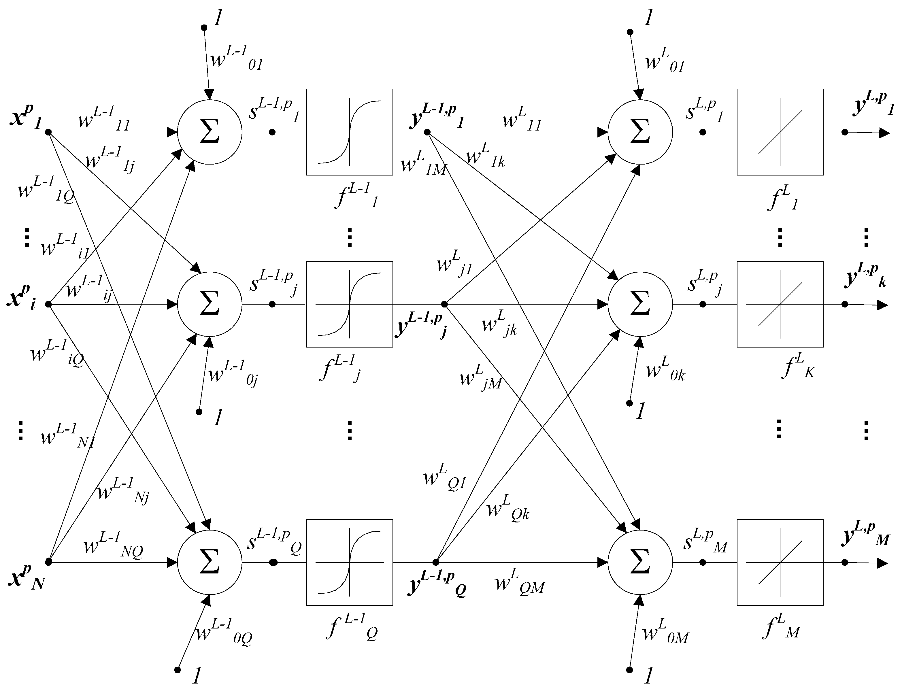
Figure 1. Architecture of a Multilayer Perceptron Neural Network with N inputs, Q neurons in the hidden layer, and M outputs.
Infrastructures 10 00301 g001
Figure 2. Example of MLP-NN architectures with one or several outputs in the output layer.
Infrastructures 10 00301 g002
Figure 3. Aerial view of Baixo Sabor dam.
Infrastructures 10 00301 g003
Figure 4. Measuring points and subsystem components of the dynamic monitoring system of the Baixo Sabor dam [28].
Infrastructures 10 00301 g004
Figure 5. Air temperature records from 2015 to 2018.
Infrastructures 10 00301 g005
Figure 6. Reservoir water level records from 2015 to 2018.
Infrastructures 10 00301 g006
Figure 7. Evolution of natural frequencies from 2015 to 2018.
Infrastructures 10 00301 g007
Figure 8. Natural frequencies estimated from experimental data and predicted values of the five MLR models from 2015 to 2018 (training and test sets).
Infrastructures 10 00301 g008
Figure 9. Architecture of an MLP-NN model with one hidden layer and one output in the output layer based on the HST approach.
Infrastructures 10 00301 g009
Figure 10. Natural frequencies estimated from experimental data and predicted values of the five MLP-NN models with one output, from 2015 to 2018 (training and test set).
Infrastructures 10 00301 g010
Figure 11. Architecture of an MLP-NN model with five outputs based on the HST approach.
Infrastructures 10 00301 g011
Figure 12. Natural frequencies estimated from experimental data and predicted values of the MLP-NN model with five outputs from 2015 to 2018 (training and test set).
Infrastructures 10 00301 g012
Table 1. Regression coefficients for the five MLR models.
Vibration Modeβ0β1β2β3
Mode 12.9543−2.2235 × 10⁻⁹−0.01009−0.004045
Mode 23.1742−2.6178 × 10⁻⁹−0.14286−0.008275
Mode 34.2382−3.8372 × 10⁻⁹−0.26121−0.018613
Mode 44.8933−4.0449 × 10⁻⁹−0.02773−0.008189
Mode 55.7554−3.9158 × 10⁻⁹−0.05067−0.034902
Table 2. Coefficient of determination and standard deviation of residuals for the five MLR models.
ModelIndicatorSetFreq. 1Freq. 2Freq. 3Freq. 4Freq. 5
R2 [%]Training92.496.995.393.581.6
Test83.491.889.684.678.5
MLR σ [Hz]Training0.01620.01160.02120.02770.0498
Test0.01630.01160.02470.03130.0550
Table 3. Coefficient of determination and standard deviation of the residuals for the MLP-NN model with one output.
ModelIndicatorSetFreq. 1Freq. 2Freq. 3Freq. 4Freq. 5
R2 [%]Training93.398.197.197.990.1
Test89.496.395.093.489.3
MLP-NN(i) σ [Hz]Training0.01520.00910.01650.02020.0386
i = 1, …, 5 Test0.01540.00860.01770.02240.0368
Number ofneurons in hidden layers [2 5][2 8][2 5][2 5][3 5]
Table 4. Coefficient of determination and standard deviation of the residuals for the MLP-NN model with five outputs.
ModelIndicatorSetFreq. 1Freq. 2Freq. 3Freq. 4Freq. 5
R2 [%]Training93.498.597.496.889.3
Test83.392.392.590.088.6
MLP-NN(1,2,3,4,5) σ [Hz]Training0.0150.0080.0160.020.038
Test0.0170.0110.0210.0250.041
Number of neurons in hidden layer [10]
Disclaimer/Publisher’s Note: The statements, opinions and data contained in all publications are solely those of the individual author(s) and contributor(s) and not of MDPI and/or the editor(s). MDPI and/or the editor(s) disclaim responsibility for any injury to people or property resulting from any ideas, methods, instructions or products referred to in the content.