Article

Thermodynamics of Manufacturing Processes—The Workpiece and the Machinery

Mechanical Engineering Department, University of Texas at Austin, EnHeGi Research and Engineering, Austin, TX 78712, USA
Inventions 2019, 4(2), 28; https://doi.org/10.3390/inventions4020028
Submission received: 27 March 2019 / Revised: 30 April 2019 / Accepted: 10 May 2019 / Published: 15 May 2019
(This article belongs to the Special Issue Thermodynamics in the 21st Century)

Abstract

:
Considered the world’s largest industry, manufacturing transforms billions of raw materials into useful products. Like all real processes and systems, manufacturing processes and equipment are subject to the first and second laws of thermodynamics and can be modeled via thermodynamic formulations. This article presents a simple thermodynamic model of a manufacturing sub-process or task, assuming multiple tasks make up the entire process. For example, to manufacture a machined component such as an aluminum gear, tasks include cutting the original shaft into gear blanks of desired dimensions, machining the gear teeth, surfacing, etc. The formulations presented here, assessing the workpiece and the machinery via entropy generation, apply to hand-crafting. However, consistent isolation and measurement of human energy changes due to food intake and work output alone pose a significant challenge; hence, this discussion focuses on standardized product-forming processes typically via machine fabrication.

1. Introduction

Industrial processes—manufacturing or servicing—involve one or more forms of electrical, mechanical, chemical (including nuclear), and thermal energy conversion processes. For a manufactured component, an interpretation of the first law of thermodynamics indicates that the internal energy content of the component is the energy that formed the product [1]. Cursorily, this sums all the work that goes into the manufacturing process from electrical to mechanical, chemical, and thermal power consumption by the manufacturing equipment. However, from experience, not all of this energy goes into the material-to-product transformation. Energy dissipation (or loss) via heat generation in the machine (most machines run hot enough to require active cooling during operation) also comes from the input power. It is noteworthy that a significant fraction of the heat generation in electromechanical machines is from friction heating (mechanical) and Ohmic heating (electrical) which are both energy dissipating processes. Also, ongoing interactions with workpieces—materials from which products are made—degrade machines over time. These losses and degradation, in turn, result in significant operating costs and reduced equipment life [2]. Needed is a consistent, universal and practical approach for characterizing manufacturing processes under all operating conditions.

1.1. Least Dissipation Energy and Minimum Entropy Generation

Via Onsager’s interpretation [3], Rayleigh’s principle of least energy dissipation (L.E.D.) posits that temperature variations within a system will cause some internal energy degradation as heat flows from hot to cold regions and that the effects of any other simultaneously occurring processes are cumulative on energy degradation. Using Rayleigh’s dissipation function, Onsager expressed “dissipation” of free energy as 2Tϕ = XJ, the product of “force” X and “flow” J, where T is the temperature, ϕ is the dissipation function, and 2ϕ is equivalent to entropy production or generation S’ [3]. Assuming microscopic reversibility (via the famous reciprocal relations), Onsager applied his formulations to fluctuations of real systems undergoing linear interactions. To establish a well-defined reference for the extension of reversible (ideal or non-real) formulations to irreversible (real) systems and processes, Prigogine proposed the minimum entropy generation (M.E.G.) or stationary non-equilibrium theorem [4,5,6,7], an equivalent statement of least energy dissipation L.E.D., which suggests that systems near equilibrium or minimally perturbed from equilibrium, generate or produce minimum entropy given by S’ = XJ/T. Examples of force-flow XJ conjugate pair characterizing common systems include force-displacement Fx, pressure-volume P V , and voltage-charge Vq. It is noteworthy that while Onsager’s “free energy dissipation” includes variable phenomenological coefficients, Prigogine’s M.E.G. requires constant coefficients, making the latter truly linear or stationary.
Details of the principles of minimum entropy generation and least energy dissipation can be found in referenced texts; suffice to say that both theorems define the minimum condition for any real system or process to exist in nature (i.e., deviation from reversibility). Hence, all real systems are irreversible, and via Rayleigh’s L.E.D., energy degrades and entropy increases in the presence of internal anisotropic gradients commonly referred to as irreversibilities. The higher a system’s irreversibilities, the higher the system’s entropy production or energy degradation.

1.2. Exergy and System Irreversibilities

With energy conservation alone unable to isolate the useful portion of a system’s energy [8], thermodynamics introduces exergy, to assess a system’s available energy to do work. Often referred to as the Guoy–Stodola theorem, exergy destruction—a measure of the unavailable energy—is given as [8,9,10,11]
T0δS’ = δWrev − δWout,
the difference between maximum theoretical work δWrev and actual work δWout obtained from the system. T0, often 298 K, is the system temperature at the thermodynamic dead state: a fixed state of equilibrium with the extended surroundings assumed as a thermal reservoir (i.e., an idealized, unchanging source of energy) where T = T0, P = P0. δS’ is the entropy generation and δ indicates path dependence. The destruction of a system’s exergy or available energy during a process, Equation (1), is a direct measure of the system’s irreversibilities. As with entropy production, the destruction of a system’s exergy or available energy during a process, Equation (1), is a direct measure of the system’s irreversibilities, i.e., a system with significant irreversibilities will have high exergy destruction during the process interaction. Therefore, it is desired to keep system irreversibilities at a minimum to maximize available energy and minimize exergy destruction. However, it is noted that a system, such as a battery, could be at its lowest useful potential or exhaust its useful energy while remaining thermodynamically “alive”, far from the dead state. Also, the use of constant T0 obtained far enough from the system where the surrounding temperature is truly steady includes external irreversibilities in the portion of the surroundings between the system and the location of T0 establishment [8,9]. Moreover, if the temperature of the surroundings is significantly different from 298 K used in most availability/exergy analyses, the results are then less consistent with reality, possibly impacting the widespread usage of thermodynamics-based analysis in the degradation/performance modeling of non-thermal systems, such as electronics and electromechanical systems.
Industrial machines are typically assemblies of moving components. Investigating degradation of machinery components via thermodynamic principles, experimental studies by Bryant et al. [2,12,13] established a linear relationship between friction-induced wear and entropy transfer out of the tribological interface, under steady-state conditions. The studies, verifying that irreversible entropy production underlies permanent degradation, led to the Degradation-Entropy Generation theorem [14].

1.3. Local Equilibrium

With no known real system ever truly at equilibrium (even dead biological matter continues to decompose, eventually transforming into fossil fuel), Prigogine hypothesized that every macroscopic system is made up of elemental volumes for which observable system properties, such as temperature and pressure, can be instantaneously ascertained; as such, equilibrium formulations describing the states of these properties are valid for each elemental volume in the macrosystem. Hence, the system is in local equilibrium [4,5,6,7]. This theorem, which has since been extensively verified, further established the field of irreversible thermodynamics, allowing explicit formulations that govern real systems, similar to this study. Presented in the subsequent sections, starting from fundamental principles, is an instantaneous measure of internal irreversibilities or entropy generation in the workpiece, the workpiece-machinery interface, and the machinery, eliminating the steady-state assumption and the loopholes mentioned above in exergy analysis. Experimental verification via battery charging is subsequently presented. Here, the system refers to all the matter within the analysis boundary, e.g., an icemaker (the machine) and the water in it (the workpiece) can be defined as a composite system made up of two interacting sub-systems.

2. Product in Formation—The Workpiece

Via the first law [4,5,9,15], the energy content in a manufactured product is given by
dUp = δQp + δWp
where δQp is the net heat transfer between the component and the surroundings during manufacturing and δWp is the net work that transforms the material. Here, surroundings include machinery and the immediate vicinity of the composite system. Via the second law, the entropy change [4,5] during manufacturing is given as
dSp = (δQ / T)p + δS’p
where Tp is the component’s instantaneous absolute temperature (in K) and δS’p ≥ 0 is the entropy produced or generated in the component. The principles of minimum entropy generation and least energy dissipation also assert that δS’p ≥ 0 [3,16,17]. In Equation (3), the first right-hand side term is entropy transfer out of the component via heat. Equations (2) and (3) combine to give
dUp = TpdSp − TpδS’p + δWp
which can be re-arranged and combined with the component’s Helmholtz free energy A = U − TS [4,9,15] to give the entropy production or generation
δS’p = (δWp − dAp − SpdTp) / Tp
where
dAp = dUp − TpdSp − SpdTp
is the change in the component’s Helmholtz free energy, the differential minimum work required for product manufacture or the maximum work that can be extracted/obtained from the product in service (after manufacture). TpdSp is the heat transfer in/out of the workpiece and SpdTp is the internal energy dissipation (within the workpiece via compositional change/diffusion [4,5], or induced at the workpiece-process interface via friction or other external heating). Some non-thermal processes that are not temperature-controlled may yield a workpiece temperature rise driven by the workpiece entropy content Sp, the significance of which depends on the material properties, e.g., the coefficient of thermal expansion, melting point, and the nature of the manufacturing process. Manufacturing processes increase the workpiece’s Helmholtz energy—its utility or useful energy to do work—to a maximum (finished state), dAp ≥ 0, while reducing its overall utility-based entropy, dSp ≤ 0. Hence, the effect of the relatively low non-microstructure-changing temperature rise dTp is further minimized by the manufacturing process-reduced entropy content Sp = S0 + dSp, where S0 is the initial material entropy content. This indicates that during most non-thermal manufacture, the last term of Equation (6) can be neglected to simplify Equation (5) as
δS’p = (δWp − dAp) / Tp ≥ 0.
The actual work δWp includes dissipative phenomena at the machine-workpiece interface that do not contribute to the product’s desired final form, e.g., using a non-ideal cutting tool for a machining task will increase δWp for a given dAp, and in turn, the entropy generation δS’p is increased. Therefore, it is easily inferred that a low δS’p is desirable. As mentioned previously, the second law prohibits negative entropy generation in all real systems/processes, i.e., δS’p ≥ 0 or δWp ≥ dAp, establishing δS’p = 0 or δWp = dAp as the limit of possibility or ideal (reversible) case. In other words, conforming with everyday experience, one cannot obtain from the product more than what has gone into its formation (efficiency ≥ 100% is unattainable), a corollary of the second law known as the Carnot limitation [10]. Equation (7) further indicates that the ideal case is only possible under perfectly isothermal conditions dTp = 0.

3. Manufacturing Equipment and Process—The Machinery

In addition to characterizing and detecting unusual phenomena at the machine-workpiece interface, of significant interest are the efficiency and degradation of the manufacturing equipment and process. As done for the workpiece, the energy balance of the machinery is
dUm/c = δQm/c + δWm/c
where the net machine work (work that changes/degrades the machine) is
δWm/c = δWin − δWp,
the difference between the input work (e.g., power supplied to the lathe or the CNC machine during operation) and the actual product formation work. Equation (9) indicates that some of the input power is lost between the input point and the machine-workpiece interface. Hence, a low δWm/c is always desired. δWm/c includes all the energy conversion losses, friction, Ohmic dissipation, corrosion, plasticity, and shaft misalignment effects, and should be resolved into appropriate constituents based on an order of magnitude analysis of the specific system or manufacturing process. Combined energy and entropy balance on the machinery (substituting entropy balance and Equation (9) into Equation (8)) yields
dUm/c = Tm/c (dS − δS’)m/c + δWin − δWp.
Rearranging with the Helmholtz free energy change dAm/c = dUm/c − Tm/cdSm/c − Sm/cdTm/c, the entropy generation in the machinery is
δS’m/c = (δWin − δWp − dAm/c − Sm/cdTm/c) / Tm/c ≥ 0.
Here, dAm/c is the differential ideal energy change, which can be specified via nominal machine/process specifications, or dropped if unknown, to give an instantaneous entropy generation for low-amplitude temperature changes (adequate for most pseudo-steady non-thermal processes)
δS’m/c = (δWin − δWp) / Tm/c ≥ 0,
the quotient of the difference between the machinery input work and actual interface work required to manufacture the component, and the representative machine temperature. Equation (12) includes all the dissipative phenomena taking place in the machinery during manufacture. Note that highly dissipative processes such as friction can generate significant heat, which if not transferred out via cooling, results in a substantial value of Sm/cdTm/c, a measure of the interfacial thermal fluctuations. Further breakdown of this term is given in Section 4 and references [18,19,20].
Total entropy generation in both the workpiece and the machinery, from Equations (7) and (12),
δS’total = δS’p + δS’m/c = [(δWp − dAp) / Tp] + [(δWin − δWp) / Tm/c].
If Tp ≈ Tm/c, Equation (13) becomes
δS’total = (δWin − dAp) / Tp.
δS’total, Equation (14), measures the efficiency of the entire system-process interaction and can be used as a first (overall system) analysis parameter, given its relative ease of evaluation: δWin is usually known/measurable and dAp is easily specified and typically standardized for a product and/or manufacturing task (e.g., drilling a hole in a thick steel plate or adding a thickener to grease in production)—a straight line joins the Helmholtz energy states before and after the task, an artifact of the thermodynamic state principle [4,5,8,9,15]. With a known/measured δWp, Equations (7) and (12) give the individual contributions from the workpiece and the machinery respectively. Further sub-system analyses can be performed as necessary to determine the significant sources of irreversibilities in the process.

4. Entropy Content S and Internal Free Energy Dissipation–SdT

The Helmholtz relation—Equation (6) and the subsequent version for the machinery—introduced “–SdT”, the portion of the free energy dissipated and accumulated internally by a loaded component, which includes effects of plastic work, chemical reaction heat generation, and sometimes heat from an external source [18,19,20]. Temperature change dT is driven by the system entropy content S. Without an entropy measurement device, S is often neglected in thermodynamic formulations characterizing real systems, justified by setting dT = 0, which in turn requires experiments to be isothermal for validation, and significant temperature correction for application to real-world operation. With δW = YX, Equation (6) A = A(T,X,N) suggests the Helmholtz entropy content SA = S(T,X,N) [15]: entropy of a system depends on the temperature T, generalized displacement X , and number of moles N , all of which are experimentally and instantaneously measurable. Via partial derivatives, the Helmholtz entropy change for a system with one reactive species is
dS = ( S T ) X , N dT + ( S X ) T , N dX + ( S N ) T , X dN
From Maxwell’s thermodynamic manipulation of mixed partial second derivatives of the fundamental energy relations and Callen’s derivatives reduction technique [15], Equation (15) can be restated using derived measurable system parameters [4,15] in terms of generalized variables X and Y as
( S T ) X , N = C X T ;   ( S X ) N , T = ( Y T ) X , N = α κ T ;   ( S N ) T , X = ( μ T ) X , N
where C X is the heat capacity (for solids, C X C Y = C ), α = 1 X ( X T ) Y , N > 0 is the generalized coefficient of thermal expansion, and κ T = 1 X   ( X Y ) T , N > 0 is the generalized isothermal loadability [18], obtained via the application of Callen’s technique [15] to the isothermal Helmholtz derivative, ( A Y ) T , N = X to give ( 2 A Y 2 ) T , N = X κ T , a system/material property. μ T is the reaction potential-temperature gradient, also obtained for batteries, with μ = V , by Osara et al. via the Gibbs–Duhem formulation [20]. While C and α , measuring system response to heat and temperature changes, retain consistent meanings in all systems, generalized κ T represents the isothermal loadability, a measure of the material/component’s “cold” response to boundary loading. Substitute Equation (16) into Equation (15) to give
dS = C X T dT + α κ T dX μ T dN .
Integrating with initial condition S 0 = 0 yields instantaneous entropy content
S = C X ln T + α κ T X Δ μ Δ T N ,
as a function of easily observable and measurable system-process parameters T, X, N and easily determinable material properties C X , α , κ T , μ .
From the above, internal free energy dissipation
SdT = ( C X ln T + α κ T X Δ μ Δ T N ) dT
which measures thermal instabilities during the system-process interaction, for processes with significant temperature changes. As indicated previously, note that with the decreasing entropy S of a product in formation, –SdT is typically more significant in the machinery than the workpiece. However, for non-thermal manufacturing processes with minimal temperature rise, an order of magnitude analysis shows –SdT can often be neglected.

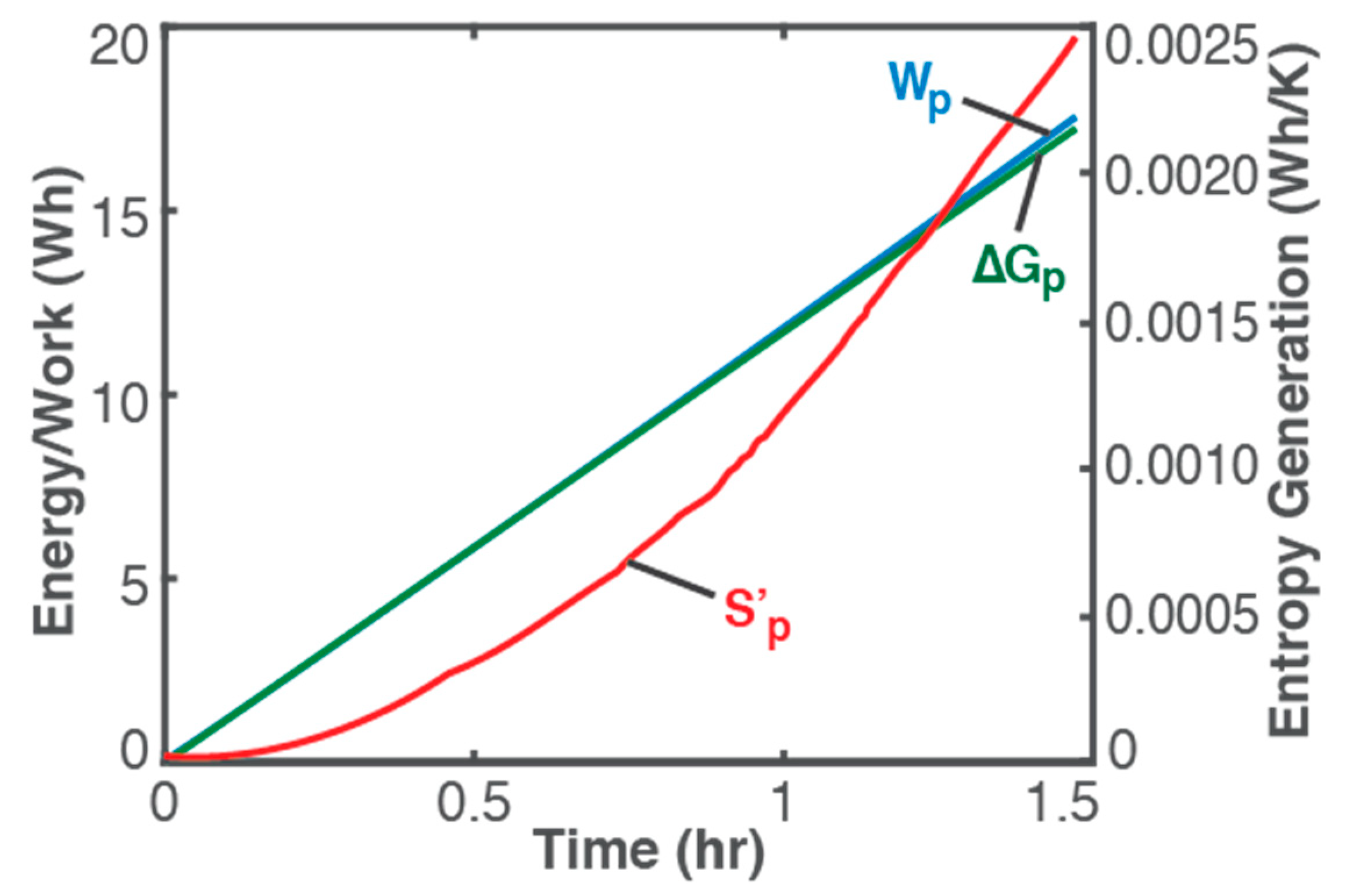
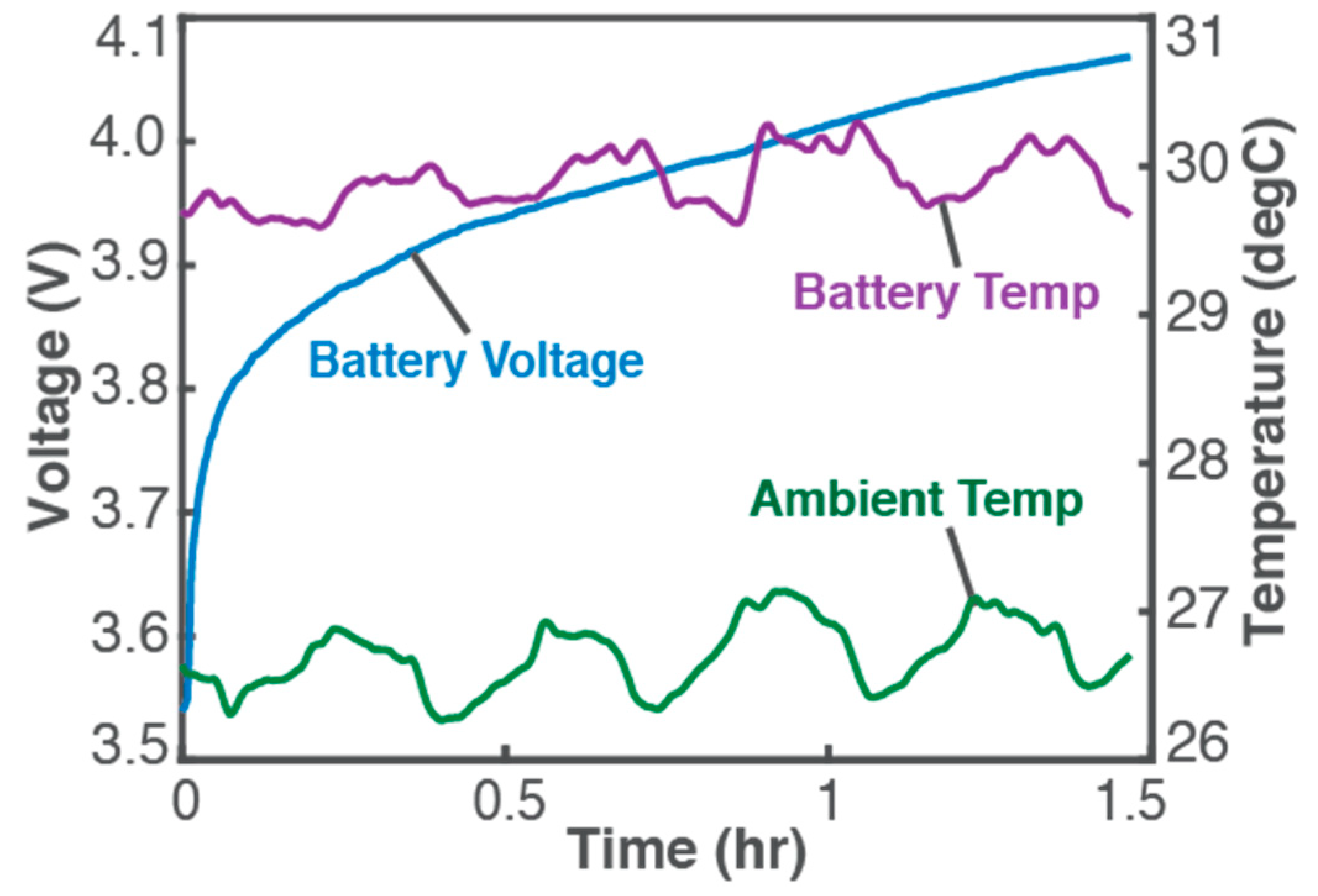
5. Battery Charging and Other Example Processes

Figure 1 plots experimental data from a 3.7 V, 11 Ah Li-ion battery undergoing constant-current charge [1,20] (energy-adding process) for which Equation (7) gives the entropy generation in the battery, in terms of voltage V (blue plot in Figure 1, left axis), constant current I = 3 A, battery temperature T (purple plot in Figure 1, right axis), over time t, as
S = ( t VI dt V 0 C rev ) / T 0
where Ohmic work Wp = ∫t VI dt (blue plot in Figure 2, left axis), can be determined via knowledge of the charging process, readily obtained from measurements. Similar to the Helmholtz free energy ∆Ap for non-reactive and non-thermal systems, the minimum recharge energy required for a battery or other electrochemical energy device is its Gibbs free energy ∆Gp = V0 C rev (green plot in Figure 2, left axis), determined via knowledge of the battery: V0 is the battery’s standard potential and C rev can be evaluated using Faraday’s first law [4,20]. In terms of chemical potential and number of moles or reaction affinity and extent [4,9], change in Gibbs potential ∆Gp characterizes the chemical formation of products, a standardized form of which is the so-called Gibbs free energy of formation of certain pure substances. For a thermally dominant process, enthalpy ∆Hp is the minimum thermal energy required for product formation, which has also been standardized as the enthalpy of formation.
It is observed (from Figure 1) that instantaneous temperature changes are slow and appear indicative of ambient conditions (see ambient temperature, green plot and right axis), with a negligible overall temperature change during charge: a low-rate (0.26 C in this case) charge process will proceed at pseudo-steady temperature as anticipated in the above discussions and represented in Equation (20). In Figure 2, plots of the accumulated Ohmic work Wp (blue plot, left axis), Gibbs free energy ∆Gp (green plot, left axis), and entropy generation S’p (red plot, right axis), via Equation (20), obtained from measured V and T with constant I of 3 A, verify the above formulations:
  • Wp ≥ ∆Gp and S’p ≥ 0 for a product-forming or energy-adding process; and
  • as Wp → ∆Gp, S’p → 0 and ∆T → 0, limit of which is the reversible transformation, i.e., Wp = ∆Gp, S’p = 0 and ∆T = 0.
For manufacturing processes that deform the workpiece (elastically and plastically), δWp = V σdε where V is the volume, σ is stress, and ε is strain [18,21]; dAp = σ’fd(σ’f/E), a constant, where σ’f is the fatigue strength coefficient and E is Young’s modulus. Similarly, δWp for other processes can be expressed in terms of process-defining variables or characterized using the specific process energy as done in [22,23] for cutting and grinding processes and accompanying dAp specified in similar parameters as done above for battery charging and material deformation.

6. Product in Use

After manufacturing, an opposite process begins at the start of product use. Manufacturers and consumers are primarily concerned with a product’s usability and durability. The product’s free energy measures the usability [4,8,9] of the product while entropy production, a measure of its degradation [14,20,24], determines its performance. Following a similar procedure as that of the product formation analysis, entropy generation during product use is
δS’p = (dAp − δWout) / Tp ≥ 0
where dAp and δWout are the product’s maximum and actual work outputs, respectively. More details on dissipative entropy generation during system/product operation can be found in [1,14,18,19,20,24].

7. Entropy: Generation or Change

Unlike the non-negative entropy generation δS’, entropy change dS can be negative or positive: S is a state variable whereas S’ is a path or evolution variable [4,5,15]. From Equation (4),
dSp = (dUp + TpδS’p − δWp) / Tp ≤ 0,
indicating (dUp + TpδS’p) ≤ δWp, the input product formation work at the machine-workpiece interface δWp must be greater than or equal to the sum of the required energy content of the finished product dUp and the workpiece irreversibilities TpδS’p. However, according to the second law of thermodynamics, the process described by Equation (22) is not possible unless the total—workpiece and machine—entropy is monotonically non-decreasing, expressed as
dStotal = dSp + dSm/c ≥ 0.
A comparison of Equations (22) and (23) indicates that the overall entropy of the machine Sm/c (and that of the immediate vicinity considering the entropy transfer out via heat, see Equation (3)) will increase by an amount greater than or equal to the reduction in the component’s entropy via the manufacturing process.

8. Utility vs. Availability Analysis—Local Equilibrium vs. Thermodynamic Dead State

Equation (1), defining exergy destruction, appears similar to Equation (21) and the converse version in Equation (7) (with δWrev ~ dAp). However, it is noteworthy that Equations (1) and (20) will give different results under conditions where the component temperature Tp is a variable on the “phenomenological” path, i.e., Tp ≠ T0, allowing for more accurate and consistent evaluation of internal irreversibilities within the system of interest only, while considering changes in the surroundings and the system’s thermal characteristic. The use of constant T0 obtained far enough from the system where the temperature of the surroundings is truly steady can include significant external irreversibilities in the portion of the surroundings between the system and the location of T0 establishment [8,9].
Exergy, measuring the system’s available energy with respect to a fixed equilibrium (or dead) state, is evaluated before and after process completion, whereas this study, via thermodynamic free energies, applies Prigogine’s local equilibrium assumption to the instantaneous evaluation of entropy generation in the manufacturing/formation process.

9. Fluctuations and Instabilities

While minimum entropy generation (M.E.G.) and least energy dissipation (L.E.D.) are only valid in the “neighborhood” of equilibrium, Equation (5): δS’p = (δWp − dAp − SpdTp) / Tp, and Equation (11): δS’m/c = (δWin − δWp − dAm/c − Sm/cdTm/c) / Tm/c ≥ 0, give entropy generation in real systems far from equilibrium. Note that for an instantaneous application, dAp and dAm/c can be considered insignificant—both are elemental (differential) constants. For many real systems and processes (not merely existing at the “least dissipation” state), high-amplitude instantaneous fluctuations mean fast changing δW, S, and T, interactions included in Prigogine’s “local” potential formulation [4,5,6,7], developed for far-from-equilibrium transformations, which has been shown, via Equation (19), to be an equivalent expression of the –SdT term present in above formulations for real systems experiencing significant temperature changes during work interactions [18,19]. Unlike Equation (19) and Prigogine’s stability equation, Onsager’s reciprocity relations [3] do not apply to far-from-equilibrium interactions. With less fluctuations indicating stability, system optimization can be performed by minimizing –SdT, the limit of which leads to L.E.D. and M.E.G. Optimization strategies based on entropy generation minimization have been proposed by Bejan [25,26]. Equation (19) is central to the current work by the author on the degradation of all real systems [18,19,20,27].

10. Conclusions

Based on foundational irreversible thermodynamics, the formulations derived in this article present convenient and consistent ways of assessing a manufacturing process, sub-process, and multiple simultaneously occurring processes, via the workpiece and the machinery, using utility-based entropy generation (Equations (7), (11), and (14)). Thermodynamic free energies conveniently encapsulate energy transfer via heat, measure internal irreversibilities only, and are especially useful when heat capacities and heat exchanges with the environment during manufacture are unknown or difficult to measure accurately. It was shown that utility-based entropy generation could instantaneously measure the wastage/losses in any system-process interaction, a knowledge of which is critical to improving the system and process efficiencies, and reducing costs; an efficient process minimizes its entropy generation, indicating a low S’ is preferred. Data from experimental Li-ion battery charging verified the theoretical formulations.

Funding

This research received no external funding.

Conflicts of Interest

The author declares no conflict of interest.

Abbreviations

NomenclatureNameUnit
AHelmholtz free energyJ
GGibbs energyJ, Wh
Idischarge/charge current or rateA
QheatJ
Sentropy or entropy contentJ/K, Wh/K
S’entropy generation or productionJ/K Wh/K
ttimesec
TtemperaturedegC or K
Uinternal energyJ
VvoltageV
V volumem3
WworkJ
Subscripts & acronyms
0constant or initial reference
pproduct, workpiece, component
m/cmachine, machinery
totaltotal
ininput
outoutput
revreversible

References

  1. Osara, J.A. The Thermodynamics of Degradation. Ph.D. Thesis, The University of Texas at Austin, Austin, TX, USA, May 2017. [Google Scholar] [CrossRef]
  2. Doelling, K.L.; Ling, F.F.; Bryant, M.D.; Heilman, B.P. An experimental study of the correlation between wear and entropy flow in machinery components. J. Appl. Phys. 2000, 88, 2999–3003. [Google Scholar] [CrossRef]
  3. Onsager, L. Reciprocal Relations in Irreversible processes 1. Am. Phys. Soc. 1931. [Google Scholar] [CrossRef]
  4. Kondepudi, D.; Prigogine, I. Modern Thermodynamics: From Heat Engines to Dissipative Structures; John Wiley & Sons Ltd.: Hoboken, NJ, USA, 1998. [Google Scholar]
  5. Prigogine, I. Introduction to Thermodynamics of Irreversible Processes; Charles C. Thomas Pulisher: Springfield, IL, USA, 1955. [Google Scholar]
  6. Nicolis, G.; Wiley, J. Self-Organization in Nonequilibrium Systems: From Dissipative Structures to Order through Fluctuations; Wiley: New York, NY, USA, 1977; pp. 339–426. [Google Scholar]
  7. Glansdorff, P.; Prigogine, I. Thermodynamic Theory of Structure, Stability and Fluctuations; Wiley-Interscience: Hoboken, NJ, USA, 1971. [Google Scholar] [CrossRef]
  8. Moran, M.J.; Shapiro, H.N. Fundamentals of Engineering Thermodynamics, 5th ed.; Wiley: Hoboken, NJ, USA, 2004. [Google Scholar]
  9. Bejan, A. Advanced Engineering Thermodynamics, 3rd ed.; John Wiley & Sons Inc.: Hoboken, NJ, USA, 1997. [Google Scholar]
  10. Burghardt, M.D.; Harbach, J.A. Engineering Thermodynamics, 4th ed.; HarperCollinsCollege Publishers: New York, NY, USA, 1993. [Google Scholar]
  11. Pal, R. Demystification of the Gouy-Stodola theorem of thermodynamics for closed systems. Int. J. Mech. Eng. Educ. 2017, 45, 142–153. [Google Scholar] [CrossRef]
  12. Bryant, M.D. Entropy and dissipative processes of friction and wear. FME Trans. 2009, 37, 55–60. [Google Scholar]
  13. Ling, F.F.; Bryant, M.D.; Doelling, K.L. On irreversible thermodynamics for wear prediction. Wear 2002, 253, 1165–1172. [Google Scholar] [CrossRef]
  14. Bryant, M.D.; Khonsari, M.M.; Ling, F.F. On the thermodynamics of degradation. Proc. R. Soc. A Math. Phys. Eng. Sci. 2008, 464. [Google Scholar] [CrossRef]
  15. Callen, H.B. Thermodynamics and an Introduction to Thermostatistics; John Wiley & Sons, Ltd.: Hoboken, NJ, USA, 1985. [Google Scholar]
  16. De Groot, S.R. Thermodynamics of irreversible processes. J. Phys. Chem. 1951, 55, 1577–1578. [Google Scholar] [CrossRef]
  17. De Groot, S.R.; Mazur, P. Non-Equilibrium Thermodynamics; Dover Publications: New York, NY, USA, 2011. [Google Scholar]
  18. Osara, J.A.; Bryant, M.D. Thermodynamics of fatigue: degradation-entropy generation methodology for system and process characterization and failure analysis. Entropy 2019. under review. [Google Scholar]
  19. Osara, J.A.; Bryant, M.D. Thermodynamics of grease degradation. Tribol. Int. 2019. in print. [Google Scholar]
  20. Osara, J.A.; Bryant, M.D. A thermodynamic model for lithium-ion battery degradation: application of the degradation-entropy generation theorem. Inventions 2019, 4, 23. [Google Scholar] [CrossRef]
  21. Morrow, J. Cyclic Plastic Strain Energy and Fatigue of Metals. In Internal Friction, Damping, and Cyclic Plasticity; ASTM International: West Conshohocken, PA, USA, 1965. [Google Scholar]
  22. Bryant, M. Unification of friction and wear. Recent Dev. Wear Prev. Frict. Lubr. 2010, 248, 159–196. [Google Scholar]
  23. Kalpakjian, S. Manufacturing Processes for Engineering Materials, 2nd ed.; Addision-Wesley: Boston, MA, USA, 1991. [Google Scholar]
  24. Naderi, M.; Amiri, M.; Khonsari, M.M. On the thermodynamic entropy of fatigue fracture. Proc. R. Soc. A Math. Phys. Eng. Sci. 2010, 466. [Google Scholar] [CrossRef]
  25. Bejan, A. The method of entropy generation minimization. In Energy and the Environment; Springer: Dordrecht, The Netherlands, 1990; pp. 11–22. [Google Scholar]
  26. Bejan, A.; Tsatsaronis, G.; Moran, M. Thermal Design and Optimization; Wiley: Hoboken, NJ, USA, 1999. [Google Scholar] [CrossRef]
  27. EnHeGi. Available online: https://www.enhegi.com (accessed on 3 March 2019).
Figure 1. Monitored parameters during a 1.5 h constant-current charge of a 3.7 V, 11 Ah Li-ion battery at 3 A. Reproduced from [1]. Experimental details are available in [1,20].
Inventions 04 00028 g001
Figure 2. Ohmic work Wp = ∫t VI dt (blue plot, left axis), Gibbs free energy ∆Gp = V0qrev (green plot, left axis), and entropy generation S’p from Equation (20) (red plot, right axis) during a 1.5 h constant-current charge of a 3.7 V, 11 Ah Li-ion battery of 3 A.
Inventions 04 00028 g002

