A Wind Power Prediction Approach on the Grounds of FCM Fuzzy Clustering and TCN–Transformer

Abstract

With the goal of achieving more accurate wind power predictions by accounting for meteorological influences comprising wind speed, together with wind direction and air pressure, this thesis proposes a method combining fuzzy C-means (FCM) clustering with a TCN–Transformer hybrid model. After preprocessing the data to remove outage and missing records, we apply the Pearson correlation coefficient to identify average wind speed and wind direction that are suitable to serve as input features for the model, together with the atmospheric pressure, as key input features. FCM clustering is then applied to partition the data into low- and high-wind-speed operating conditions, mitigating the accuracy loss caused by uniform modeling. A TCN–Transformer model is subsequently constructed, integrating local temporal feature extraction with global dependency modeling to perform prediction under each condition. The experimental results demonstrate that the proposed FCM–TCN–Transformer framework consistently achieves superior forecasting performance under both low-wind-speed and high-wind-speed conditions. Compared with benchmark models, including TCN, LSTM, GRU, BiGRU, and Transformer, the proposed method achieves lower prediction errors and higher prediction accuracy across different forecasting horizons. Furthermore, repeated experiments with multiple random seeds verify the robustness and stability of the proposed framework. These results indicate that FCM-based wind regime classification effectively reduces data heterogeneity, while the hybrid TCN–Transformer architecture successfully captures both local temporal patterns and long-range temporal dependencies. Therefore, the proposed framework provides an effective and reliable solution for short-term wind power forecasting and contributes to the secure integration of wind energy into modern power systems.

1. Introduction

In light of the fast advancements in alternative energy, wind power now forms an integral part of the global power generation mix, as a result of its non-polluting and enduring nature [1,2]. Conversely, the stochastic, episodic, and variable characteristics of wind power, driven by multiple meteorological elements comprising air pressure, together with wind speed and wind direction, introduce significant uncertainty into power generation, introducing risks to the secure and robust operation of grid infrastructure [3]. In summary, upgrading the accuracy performance of wind energy forecasting is paramount for power grid operational scheduling and energy management [4,5].

Recent breakthroughs in machine learning have provided new technical pathways for wind power prediction. In particular, deep learning, feature optimization, and hybrid modeling approaches have significantly improved forecasting accuracy and model robustness [6,7]. Extensive studies have demonstrated the effectiveness of these methods across various aspects, including model development, feature selection, clustering techniques, probabilistic forecasting, and explainable artificial intelligence [8,9,10,11,12,13,14,15,16,17,18,19,20,21,22].

Within the domain of wind power prediction, selecting appropriate features is critically important, as input variables with weak correlations to power output can degrade prediction accuracy and generalization capability [23,24,25]. To address this issue, hybrid modeling and feature engineering methods have been widely adopted. For example, Sharma et al. [26] showed that selecting fewer but more relevant features can effectively reduce overfitting and computational complexity, while principal component analysis-based feature construction further enhances prediction performance [27]. In addition, due to the significant variability in wind turbine operating conditions under different wind regimes, unified models often fail to accurately capture power variation patterns, leading to reduced prediction accuracy [28,29,30]. Consequently, classifying wind power data according to meteorological characteristics has become an effective approach for improving model performance [31].

Regarding data classification, conventional hard clustering algorithms, such as K-means and K-medoids, assign each sample to a single category [32,33,34]. However, these methods fail to capture the continuous transitions between operating conditions. Studies have shown that wind power data exhibit inherent fuzzy characteristics, particularly in transition regions between different wind speed intervals [35]. To address this limitation, fuzzy clustering methods, including the FCM algorithm (fuzzy C-means) and the PCM approach (possibilistic C-means), have been introduced. These methods assign membership degrees to multiple clusters, better reflecting the intrinsic distribution of wind power data and improving classification robustness [36,37]. Existing studies have demonstrated that FCM-based classification can effectively capture differences in turbine output characteristics and significantly improve prediction accuracy compared to unified models [29,38,39,40,41]. Furthermore, advanced fuzzy clustering approaches, such as interval type-2 fuzzy possibilistic C-means, further enhance robustness under uncertainty [42]. Although existing studies have demonstrated the effectiveness of FCM-based classification for wind power forecasting, most of them focus primarily on improving data partitioning strategies or integrating FCM with a single forecasting architecture. However, wind power series exhibit both local temporal fluctuations and long-range dependencies, which are difficult to characterize using a single feature extraction mechanism. Consequently, there is still room for further improving forecasting accuracy under different wind operating conditions.

To address these issues, this study integrates FCM-based wind regime classification with a hybrid TCN–Transformer forecasting framework. The FCM algorithm is employed to reduce the heterogeneity of wind power data by distinguishing different operating regimes. Subsequently, the TCN module is used to extract local temporal features, while the Transformer encoder captures long-range temporal dependencies through the self-attention mechanism. By combining wind regime classification with complementary temporal feature extraction, the proposed framework aims to achieve more accurate and robust wind power forecasting under different operating conditions.

Regarding prediction models, traditional avenues including back propagation (BP) networks and long short-term memory architecture have become a popular choice in many studies. However, BP networks are predisposed to locally optimal solutions and lack the effectiveness to model temporal dependencies effectively [43], while LSTM models have the problems of high computational complexity and low efficiency in handling long sequences [44,45]. Similarly, the family of recurrent neural networks, including their many variations, such as Gated Recurrent Units (GRUs), is affected by gradient vanishing and exploding problems [46]. Convolution-based models, including Convolutional Networks (CNNs) and Temporal Convolutional Networks (TCNs), have also been explored. While CNNs perform well at capturing local features, they fall short when it comes to learning relationships over extended time horizons [47]. TCNs address this issue through causal and dilated convolutions, enabling larger receptive fields, but still face limitations in capturing global features and multi-scale patterns [48,49,50]. More recently, the self-attention-driven Transformer family of models has demonstrated superior capability for capturing global dependencies within time series [51,52]. Nevertheless, Transformers rely on massive datasets and marked computational resources and are less effective at capturing local fine-grained features [46]. Consequently, hybrid approaches that unify the beneficial aspects of multiple approaches have become an important investigative direction [53,54,55].

Based on the above analysis, this study makes the following main contributions:

• Wind regime classification based on fuzzy clustering: An FCM-based wind regime classification strategy is introduced to partition wind power data into low- and high-wind-speed operating conditions. Compared with conventional hard clustering approaches, the fuzzy membership mechanism better characterizes the transition regions between different operating states and reduces data heterogeneity before forecasting.
• A hybrid TCN–Transformer forecasting framework: A hybrid forecasting model is developed by integrating Temporal Convolutional Networks (TCNs) and Transformer encoders. The TCN module is responsible for extracting local temporal patterns, while the Transformer encoder captures long-range dependencies through the self-attention mechanism. The complementary strengths of the two components enable more effective modeling of complex wind power dynamics.
• Comprehensive validation under different forecasting horizons and wind regimes: The proposed framework is evaluated using real SCADA data collected from a wind farm in Gansu, China. Forecasting performance is assessed over 12 h, 24 h, and 72 h horizons under both low- and high-wind-speed conditions. Experimental results demonstrate that the proposed method consistently achieves superior forecasting accuracy compared with several representative deep learning models, including TCN, LSTM, and Transformer.

The remainder of this paper is organized as follows. Section 2 describes the materials and methods, including data preprocessing, feature correlation analysis, FCM clustering, and the architecture of the proposed TCN–Transformer hybrid model. Section 3 presents the experimental setup and the comparative results of different models under low- and high-wind-speed conditions. Section 4 discusses the findings, including the limitations and practical implications. Section 5 concludes the paper with a summary of the main contributions and future work.

2. Materials and Methods

2.1. Classification of Wing Turbine Operating Conditions Based on Fuzzy C-Means Clustering

2.1.1. Data Preprocessing

The power produced by wind turbines is largely determined by wind speed, approaching zero at low wind speeds and remaining constant under cut-out conditions. Additionally, during operation, faults, shutdowns, or abnormal power outputs may occur. Raw SCADA data typically contain missing values, shutdown records, and outliers that deviate from the normal wind speed–power relationship. If such anomalous data are directly used in prediction models, they can adversely affect the precision and resilience of the model in forecasting.

To ensure that the data of the wind power estimation model were of a good quality, the unprocessed data of wind rate and power were preprocessed and cleaned in the context of this study. The data cleaning process involved the following operations:

(1)

Missing Data Processing: Data entries that have missing values (NaN) were removed from the dataset to ensure data integrity.

(2)

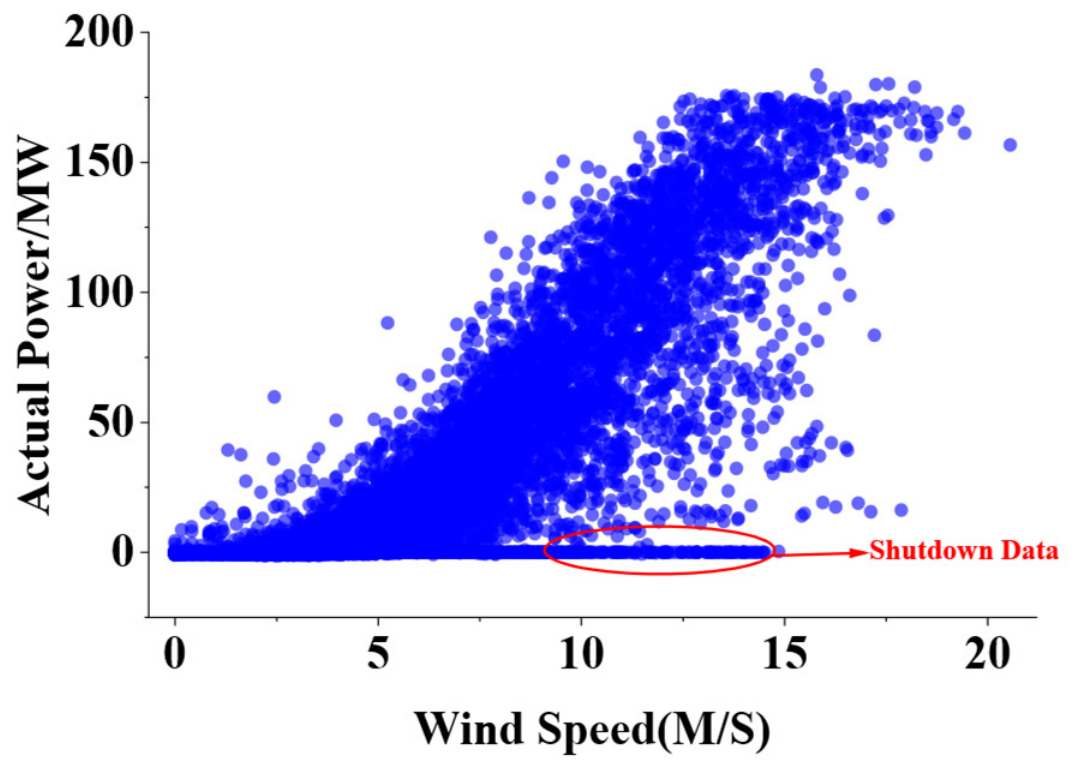
Removal of Shutdown Data: Records with actual power less than or equal to zero were discarded, as such data do not reflect the normal operating state of the wind generator. Refer to Figure 1 for a visual representation.

The red points indicate records with power ≤ 0, which correspond to turbine shutdown, fault, or cut-out conditions. These invalid samples are removed during data cleaning to prevent negative impact on prediction model training. The remaining black points represent normal operating conditions.

2.1.2. Investigating Correlations Among Features

To thoroughly investigate the role of diverse meteorological variables on the output power of wind turbines, there is a need to quantitatively explore the correlations between the primary weather parameters and the actual power prior to constructing the model for forecasting wind power. In the current work, we chose average wind velocity, average wind bearing, atmospheric pressure, ambient temperature, and moisture content as the model’s input features. Their correlations with the actual power output were performed with the goal of isolating those variables that have a substantial impact on the magnitude of generated power.

Due to the substantial differences in the scales of various features, Z-score standardization was first applied to normalize the data, thereby preventing scale disparities from adversely affecting the clustering results:

$$X^{\prime }={\displaystyle \frac{X-\mu }{\sigma }}$$

(1)

where μ stands for the feature’s average value and σ is the amount by which the feature values deviate from the mean, on average. After standardization, each variable has zero mean and unit variance.

Subsequently, to evaluate how linearly the variables are associated, the Pearson correlation coefficient was applied. It can be written in the following way:

$$r_{xy}={\displaystyle \frac{{\displaystyle {\sum }_{i=1}^n(x_i-\overline{x})(y_i-\overline{y})}}{\sqrt{{\displaystyle {\sum }_{i=1}^n{(x_i-\overline{x})}^2\cdot \sqrt{{\displaystyle {\sum }_{i=1}^n{(y_i-\overline{y})}^2}}}}}}$$

(2)

For each sample indexed by $i$, we denote the two variable values as $x_i$ and $y_i$; the averages of these two variables across all samples are given by $\overline{x}$ and $\overline{y}$, respectively, and $r_{xy}$ represents how strongly x and y are linearly associated with each other.

For the Pearson correlation coefficient, the minimum possible value is −1 and the maximum is 1. If the coefficient is near the upper bound of 1, this reflects that the two variables move together in a strongly positive manner; in contrast, coefficients that approach the lower limit of −1 reflect a strongly inverse relationship between the variables. If the value lies near zero, it suggests that any linear connection between the variables is either very weak or practically absent.

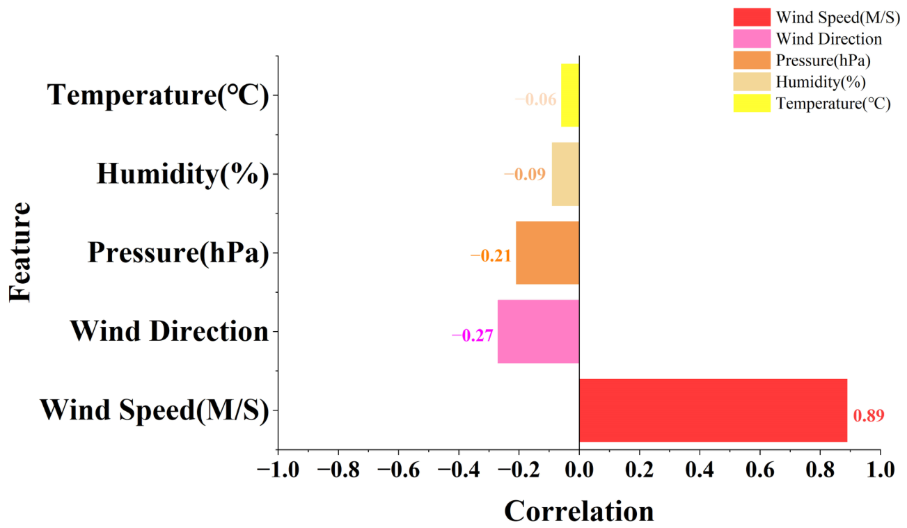
Using Equation (2), we compute the strength of correlation indicators linking each meteorological attribute to the power output, as demonstrated in Figure 2.

As shown in the figure, by analyzing the correlations between various observable weather conditions and how much power the wind turbine actually produces, it can be observed that a range of meteorological factors show substantial variation in their relative importance in determining wind power output. Among them, the average wind speed exhibits a correlation coefficient of 0.891 with the actual power output, indicating a very significant positive correlation between average wind velocity and power. This suggests that the wind turbine’s generated electrical power is most strongly governed by wind velocity, which is the overriding factor. The average wind direction shows a moderate negative correlation with the practical power output, with a correlation index of −0.274, indicating that different wind directions exert a certain effect on the efficiency of wind energy capture by the turbine. Air pressure exhibits a negative correlation with the actual power output, with a correlation coefficient of −0.209. In comparison, temperature and humidity show relatively weak correlations with power output.

Considering both the effect of climatic variables in relation to wind power output and the inter-correlations among the variables, average wind velocity, average wind direction, and barometric pressure were ultimately selected as the input feature vector for the subsequent FCM fuzzy clustering method, in addition to the primary input variables used in the wind power prediction model.

2.1.3. Fuzzy C-Means (FCM) Clustering

Owing to the significant differences in operating characteristics of wind farms under varying wind speed conditions, directly performing unified prediction on all data may reduce forecasting accuracy. Thus, before constructing the prediction model, we utilized the fuzzy C-means (FCM) clustering algorithm to separate the wind power data according to different wind condition regimes.

Fuzzy C-means (FCM) clustering is an unsupervised learning modality whose theoretical foundation is fuzzy set theory. Its core idea is that every sample may be assigned to several clusters at the same time, and the degree of membership to different clusters is represented by a membership function. Compared with traditional hard clustering methods, FCM can more clearly recognize the transitional features of wind power data across different wind conditions.

FCM minimizes the following objective function:

$$J={\displaystyle \sum _{i=1}^N{\displaystyle \sum _{j=1}^C{u}_{ij}^m{‖x_i-c_j‖}^2}}$$

(3)

where $x_i$ denotes the i-th sample, $c_j$ constitutes the j-th center of the cluster, $u_{ij}$ is the assignment probability of sample i associated with cluster j, m is the exponent controlling cluster fuzziness, and C signifies the total quantity of clusters.

Through repeated iterations, the algorithm adjusts the cluster centers along with the membership matrix. When the objective function converges, the final clustering results are obtained. We update the cluster centers using Equation (4):

$$c_j={\displaystyle \frac{{\displaystyle \sum u_{ij}^m{x}_i}}{{\displaystyle \sum u_{ij}^m}}}$$

(4)

We update the membership matrix according to Equation (5):

$$u_{ij}={\displaystyle \frac{1}{{\displaystyle {\sum }_{k=1}^C{\left(\frac{d_{ij}}{d_{ik}}\right)}^{\frac{2}{m-1}}}}}$$

(5)

Here, $u_{ij}$ is the fuzzy membership of sample $i$ to cluster $j$; $C$ is the number of clusters; $d_{ij} = \parallel x_i-v_j\parallel$ and $d_{ik} = \parallel x_i-v_k\parallel$ are Euclidean distances; and $m>1$ is the fuzzification parameter.

Finally, the wind condition categories are defined according to the magnitude of the average wind speed consistent with each cluster center.

In the FCM clustering process, the number of clusters was set to $C=2$, and the fuzzy weighting coefficient was set to $m=2$. The membership matrix was randomly initialized and normalized to satisfy the fuzzy partition constraint. The maximum number of iterations was set to 300. The algorithm terminated when the Euclidean norm between two consecutive membership matrices was smaller than ${10}^{-5}$, indicating convergence.

2.2. Wind Power Forecasting Method Based on TCN–Transformer

2.2.1. Fundamental Principles of TCN

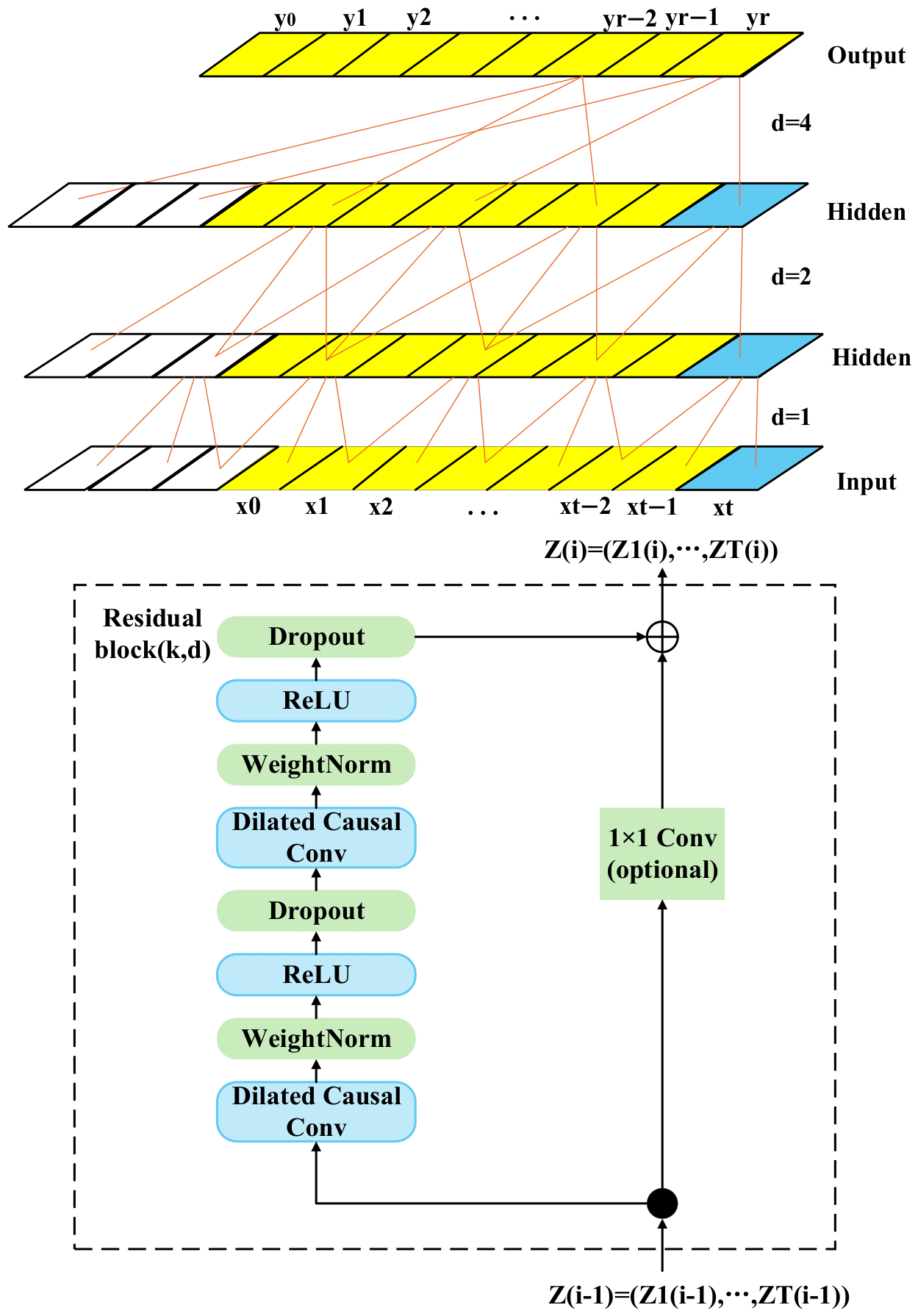
The TCN model is a CNN-based model structure whose primary purpose is sequence modeling. It ensures that predictions depend only on historical information through causal convolutions, efficiently captures long-range dependencies via dilated convolutions, and improves the stability of deep network training using residual connections. TCN has the advantage of parallel computation on time basis forecasting and has found broad application in domains like wind power prediction. The causal convolution is formulated as Equation (6):

$$y_t=\sigma \left({\displaystyle \sum _{k=0}^{K-1}{\omega }_K\cdot x_{t-k}+b}\right)$$

(6)

where $y_t$ is the output at time step $t$, $\sigma (\cdot )$ is the activation function, ${\omega }_k$ is the $k$-th convolutional kernel weight, $x_{t-k}$ is the input at time step $t-k$, $b$ is the bias term, and $K$ is the kernel size.

How dilated convolution works is mathematically described in Equation (7):

$$F\left(t\right)=\left(x\times df\right)\left(t\right)={\displaystyle \sum _{i=0}^{m-1}f\left(i\right)\cdot x_{t-d\cdot i}}$$

(7)

Here, $F\left(t\right)$ is the output of the dilated convolution at time step $t$, $x$ is the input sequence, $f$ is the convolutional filter (kernel), df denotes the dilated convolution operation with dilation factor $d$, $m$ is the filter length (number of filter taps), $f\left(i\right)$ is the $i$-th filter coefficient, $x_{t-d\cdot i}$ is the input value at time step $t-d\cdot i$, and $d$ is the dilation factor that determines the spacing between the input samples used in the convolution.

The residual connection in the TCN can be expressed as Equation (8):

$$out=x+F(x)$$

(8)

where $x$ is the input to the residual block, $F\left(x\right)$ is the output of the convolutional layers within the block, and $\mathrm{out}$ is the output after element-wise addition.

How TCN performs time series forecasting at a basic level is visualized in Figure 3.

The network consists of three key components: (1) causal convolutions, which ensure that the prediction at time step t depends only on past and current inputs (no future data leakage); (2) dilated convolutions, which exponentially increase the receptive field without increasing the number of parameters; and (3) residual connections, which add the input to the output of the convolutional layers to facilitate gradient flow and enable deeper network training. This structure allows TCN to capture long-range temporal dependencies efficiently.

2.2.2. Fundamental Principles of Transformer

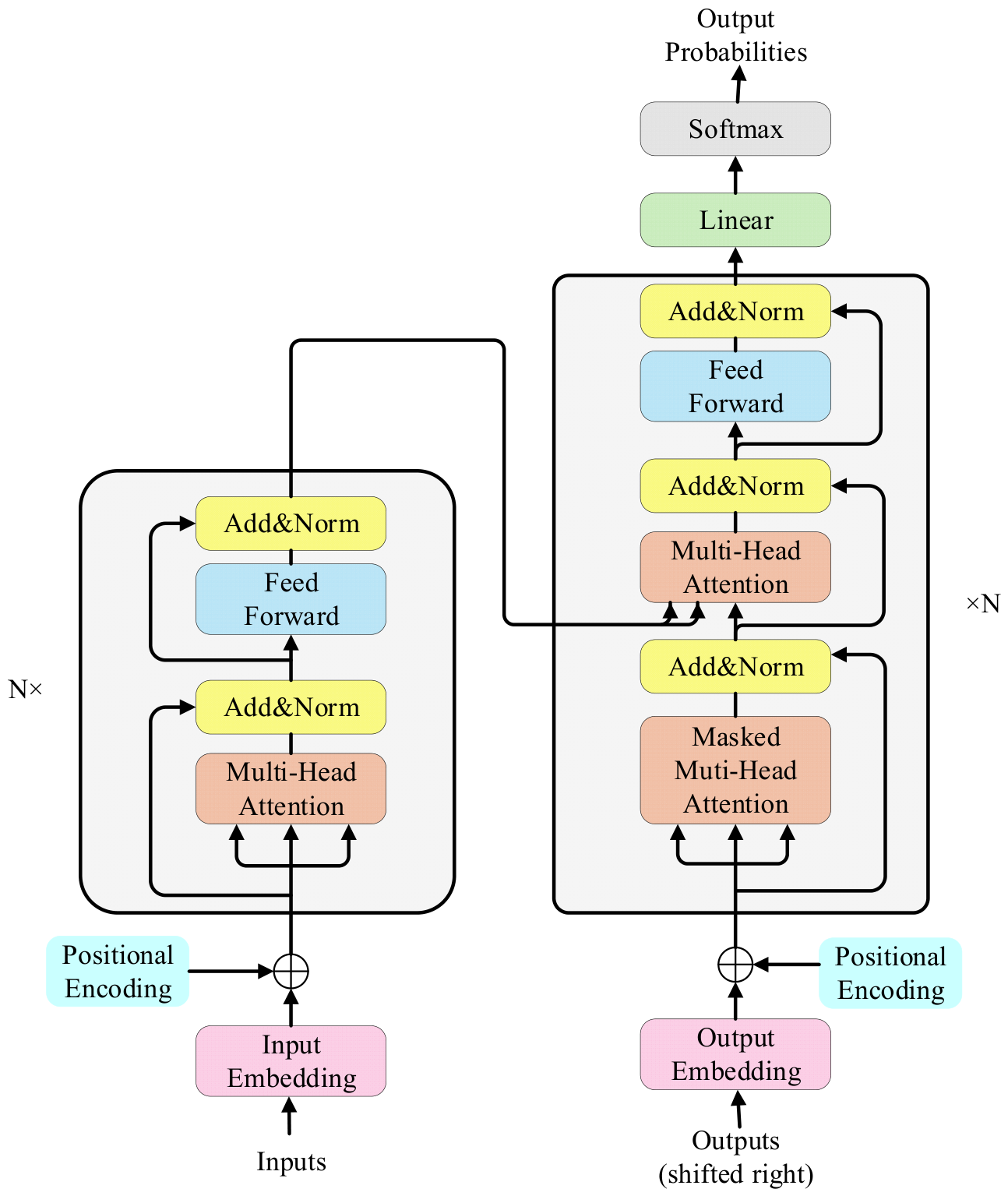
The Transformer is grounded in internal attention mechanism as its core building block. This architecture captures global temporal dependencies in chronologically ordered data without the need for cyclic network structures. It is mainly composed of a dual-module design consisting of an encoder and a decoder, where each layer includes an internal attention block with multiple heads, along with a feed-forward layer. Layer normalization together with residual connections is utilized to guarantee stable training.

Figure 4 illustrates the workflow of forecasting time series using a Transformer architecture:

The input is a sequence of historical wind power and meteorological features over a fixed time window. Each time step’s input vector is first projected into a high-dimensional embedding space, and a positional encoding is added to preserve temporal order information. The encoder consists of $L$ identical layers (here $L=2$), each containing two sub-layers: (1) a multi-head self-attention mechanism, and (2) a position-wise fully connected feed-forward network. Around each sub-layer, a residual connection is applied followed by layer normalization.

In the multi-head self-attention, the input sequence is linearly transformed into query ($Q$), key ($K$), and value ($V$) matrices. Attention scores are computed as $\mathrm{Attention}(Q,K,V)=\mathrm{softmax}\left({\displaystyle \frac{Q{K}^T}{\sqrt{d_k}}}\right)V$, where $d_k$ is the dimension of keys. Multiple attention heads operate in parallel, each capturing different types of temporal dependencies. The outputs of all heads are concatenated and linearly projected. This mechanism allows the model to directly relate any two positions in the sequence, regardless of their distance, thus capturing global dependencies across the entire input window.

The feed-forward network applies two linear transformations with a ReLU activation in between, processing each position independently. After the final encoder layer, the output features are aggregated (e.g., by taking the last time step’s output or a global average pooling) and passed to fully connected layers to produce the final wind power prediction. Unlike the full Transformer that uses a decoder for autoregressive generation, our model employs only the encoder to extract rich contextual representations from the input sequence, which are then mapped to the target power value. This design balances the ability to model long-range dependencies with computational efficiency.

2.2.3. Construction of the TCN–Transformer Model

To fully exploit the time-related characteristics and how wind power readings relate to each other across large time gaps, a hybrid forecasting model integrating TCN and Transformer is proposed in this study.

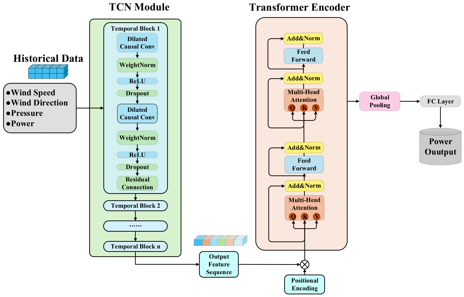
In the feature extraction stage, the model employs a TCN architecture to model the input sequence. TCN ensures temporal consistency in the time series through causal convolutions and effectively enlarges the receptive field via dilated convolutions, thereby capturing dynamic features across different time scales. Meanwhile, residual connections are introduced to keep the model stable and avoid the vanishing gradient issue that often arises when training deep networks.

On this basis, a Transformer encoder is introduced to further capture global dependencies within the sequence. Positional encoding is employed to compensate for the loss of sequential position information, and the self-attention with multiple heads is leveraged to model the correlations between distinct temporal indices, enabling the model to adaptively prioritize historical data that has a stronger bearing on the final predictions.

Finally, the output signatures of the Transformer are globally aggregated and mapped to the target space through fully connected layers to achieve wind power forecasting for future time steps.

Compared with traditional single models, the proposed TCN–Transformer model integrates local feature extraction and global dependency modeling within its architecture. TCN features strong parallel computing capability and a controllable receptive field, enabling it to efficiently capture local dynamic variations in time series data. In contrast, the Transformer overcomes sequence length limitations through the self-attention mechanism and offers significant advantages in modeling long-range dependencies.

The workflow of TCN–Transformer time series forecasting is depicted in Figure 5:

The complete workflow of the proposed FCM–TCN–Transformer method is summarized in Algorithm 1:

Algorithm 1 FCM-TCN–Transformer Wind Power Forecasting

Input: Wind power dataset D Number of clusters C = 2 Fuzziness coefficient m Maximum iterations T Time window length L Learning rate α Training epochs E Output: Predicted wind power $\widehat{\mathrm{P}}$ Evaluation metrics (NMAE, NRMSE, R2) 1:   Remove missing values and shutdown records from D 2:   Extract wind speed, wind direction, and pressure features 3:   Normalize features using Z-score standardization 4:   Initialize membership matrix U randomly 5:   for t = 1 to T do 6:      Compute cluster centers V according to Equation (4) 7:      Compute Euclidean distance matrix Dist 8:      Update membership matrix U according to Equation (5) 9:      if ||U(t) − U(t−1)|| < ε then 10:      break 11:    end if 12: end for 13: Assign each sample to the cluster with the maximum membership 14: Sort clusters according to average wind speed 15: Define: Cluster 1 → Low Wind Regime Cluster 2 → High Wind Regime 16: Split dataset D into: Dlow and Dhigh 17: for each regime Dr ∈ {Dlow, Dhigh} do 18:    Construct input sequences using sliding window L 19:    Normalize data using Min-Max scaling 20:    Build TCN module 21:    Extract local temporal features by: causal convolution dilated convolution residual connection 22:    Add positional encoding 23:    Feed features into Transformer encoder 24:    Capture global temporal dependencies using multi-head self-attention 25:    Obtain latent representation Hr 26:    Predict wind power: $\widehat{\mathrm{P}}$ = FC(Hr) 27:    Train model using MSE loss 28:    Update parameters using Adam optimizer 29: end for 30: Generate prediction results $\widehat{\mathrm{P}}$ 31: Calculate NMAE according to Equation (9) 32: Calculate NRMSE according to Equation (10) 33: Calculate R2 according to Equation (11) 34: Return $\widehat{\mathrm{P}}$, NMAE, NRMSE, and R2

2.2.4. Prediction Accuracy Evaluation Metrics

In this investigation, the estimation capability of the wind power forecasting approach is evaluated using measures such as R² (the mean coefficient of determination), as well as the standardized versions of NMAE and NRMSE.

$$NMAE={\displaystyle \frac{1}{n}}{\displaystyle \sum _{i=1}^n\frac{\left|y_i-{\stackrel{⌢}{y}}_i\right|}{y_{\max }}}\times 100\%$$

(9)

$$NRMSE={\displaystyle \frac{\sqrt{\frac{1}{n}{\displaystyle \sum _{i=1}^n{\left(y_i-{\stackrel{⌢}{y}}_i\right)}^2}}}{y_{\max }}}\times 100\%$$

(10)

$$R^2=1-{\displaystyle \frac{{\displaystyle \sum _{i=1}^n{(y_i-{\stackrel{⌢}{y}}_i)}^2}}{{\displaystyle \sum _{i=1}^n{(y_i-\overline{y})}^2}}}$$

(11)

In the above equations, $n$ is the total number of observations, $y_i$ is the actual wind power value at the $i$-th time step, ${\widehat{y}}_i$ is the predicted value, $y_{\max }$ is the maximum actual power value in the dataset, and $\overline{y}={\displaystyle \frac{1}{n}}{\sum }_{i=1}^n{y}_i$ is the mean of the actual values. The factor ×100% normalizes the errors to percentages.

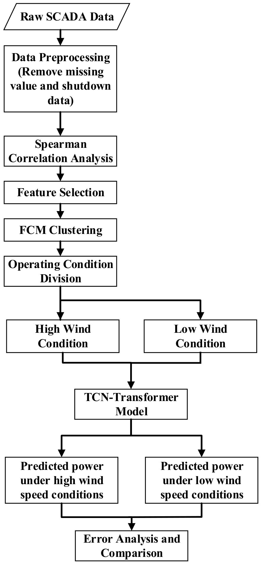
Lastly, a general description of the proposed wind power prediction procedure grounded in the fuzzy C-means approach and the TCN–Transformer hybrid model is given in Figure 6.

The procedure consists of five main stages: (1) data preprocessing, including removal of missing values and shutdown records; (2) feature correlation analysis using Pearson coefficient to select wind speed, wind direction, and air pressure as inputs; (3) FCM clustering to partition the data into low-wind-speed and high-wind-speed regimes; (4) building and training the TCN–Transformer model separately for each regime; and (5) evaluating prediction performance using NMAE, NRMSE, and R² metrics. The final output is the wind power forecast for future time steps.

3. Results

3.1. Simulation Setup

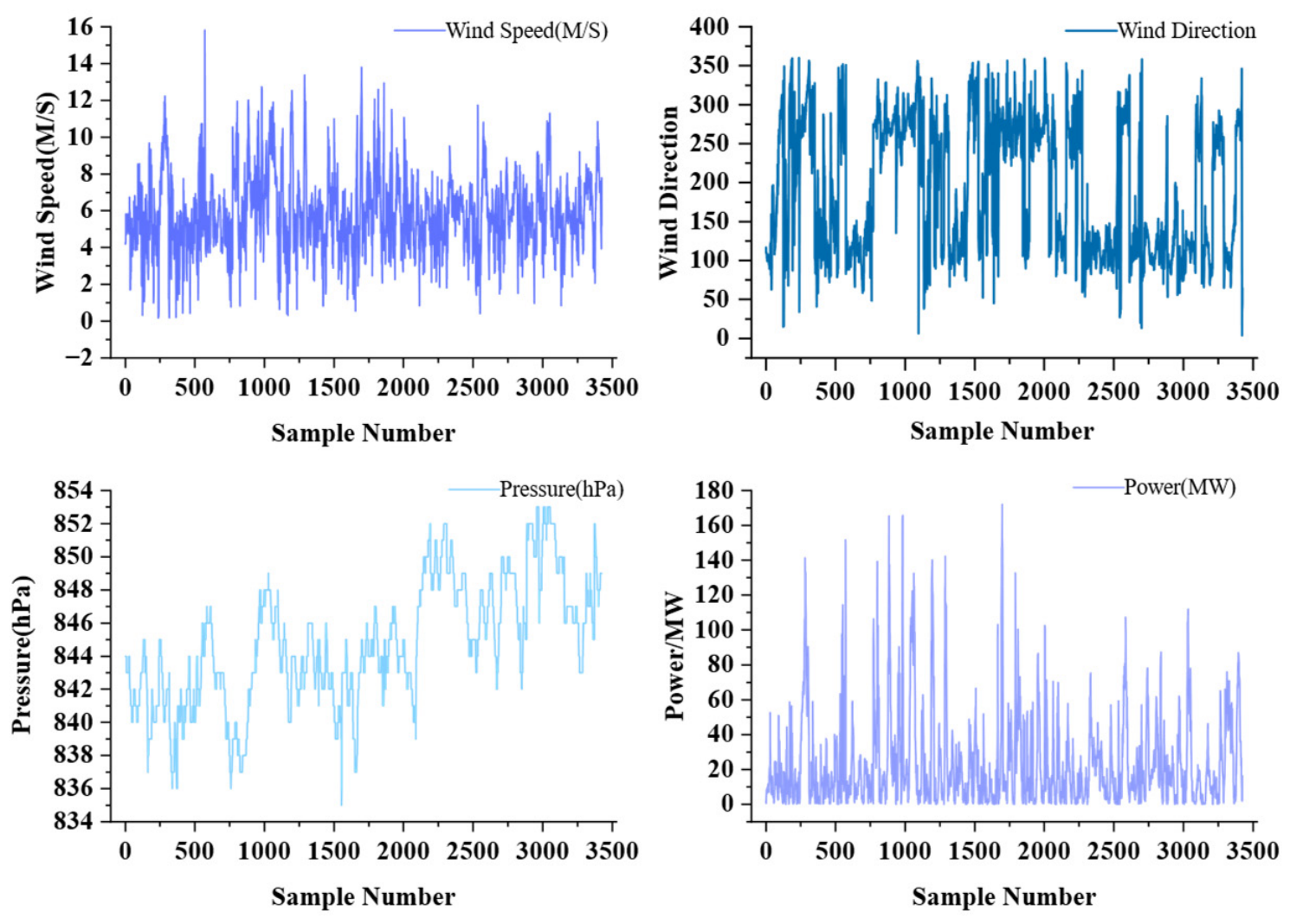
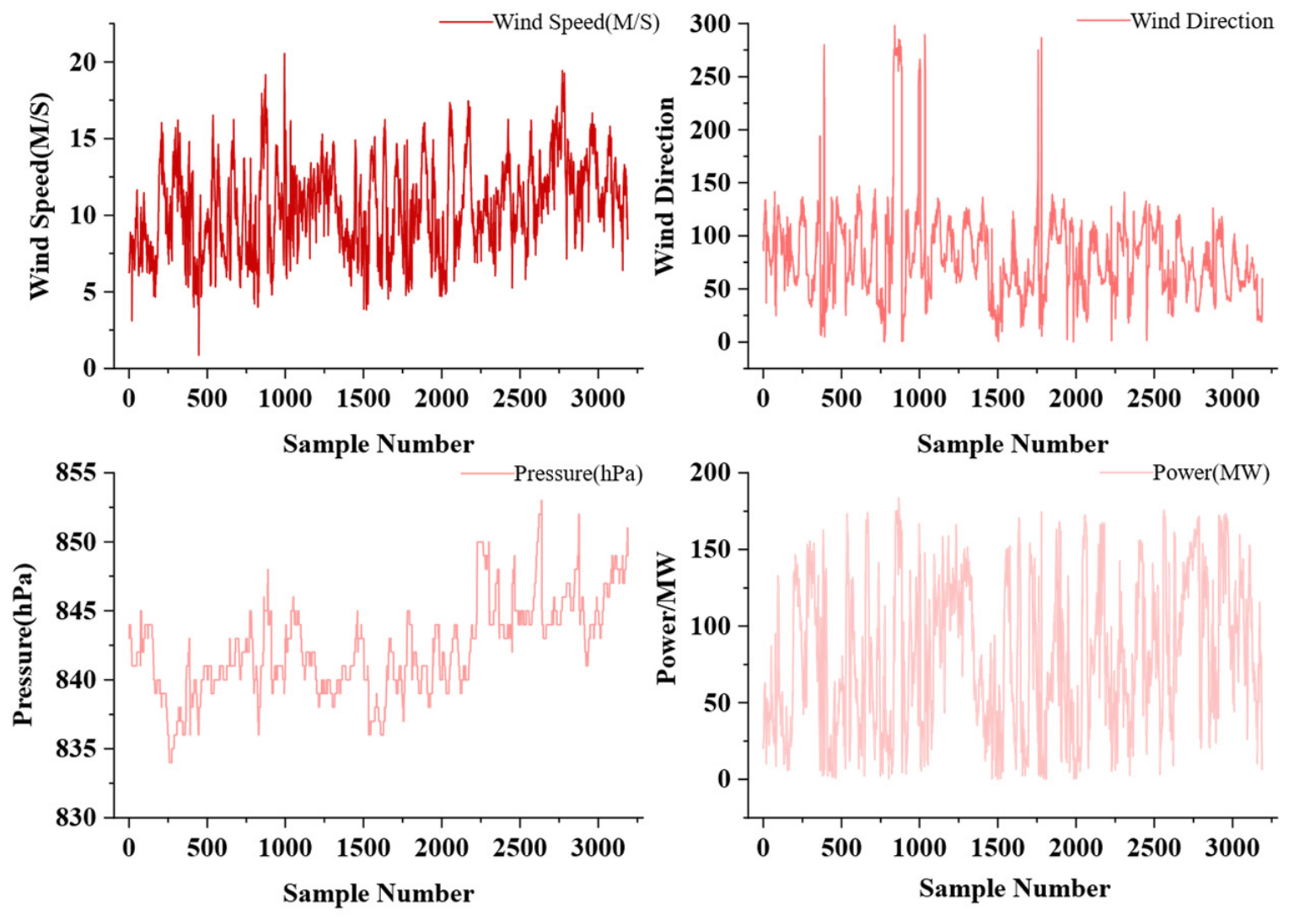
The wind power data adopted for experimental validation in this study are derived from real-world data of 126 wind turbine units in a wind power station established in Gansu, China. The wind power station consists of 101 turbines with a nominal capacity of 1.5 MW and 25 turbines with a nameplate capacity of 2 MW. The data were captured from 1 July 2020 to 1 September 2020, with data recorded every 15 min. We feed three meteorological quantities into the forecasting model we put forward: the average wind velocity (m/s), the average wind bearing, and the barometric pressure (hPa). After data preprocessing, an aggregate of 6613 samples are retained, including 3424 samples in scenarios with low wind velocity and 3189 samples in scenarios with high wind velocity. A visual representation of the low wind rate conditions is presented in Figure 7:

Figure 8 depicts the situation under high-wind-speed conditions:

3.2. Experimental Results and Comparative Evaluation

First, feature investigation is implemented to select the rate of wind movement (average, in m/s), its direction (average), and the atmospheric pressure (in hPa) as the input feature variables for the FCM clustering. We specify C = 2 for the number of clusters, the algorithm runs for at most 300 iterations, and the exponent for fuzziness (m) takes a value of 2.

On the basis of how the data were clustered, the sample data are divided into two wind condition categories. By analyzing the statistical characteristics of each category, it is found that the average wind speed exhibits the most significant difference between the two clusters. Therefore, the two categories are defined as cases with low wind speeds and cases with high wind speeds, respectively.

To verify the rationality of the selected cluster number, additional cluster validity analysis was conducted using the Silhouette coefficient, Davies–Bouldin index (DBI), and the Fuzzy Partition Coefficient (FPC). The number of clusters was varied from 2 to 6, and the corresponding results are listed in

Table 1. Cluster validity indices for different numbers of clusters.

Clusters	Silhouette	DBI	FPC
2	0.304	1.324	0.644
3	0.332	1.125	0.561
4	0.336	0.962	0.509
5	0.322	1.009	0.459
6	0.315	1.073	0.422

.

As shown in Table 1, the highest Silhouette coefficient (0.336) and the lowest DBI (0.962) were obtained when C = 4, indicating slightly better cluster compactness and separation. However, the performance improvement compared with C = 2 was relatively limited. In contrast, the maximum FPC value (0.644) was achieved when C = 2, suggesting a more stable fuzzy partition.

Considering that the objective of this study is to distinguish representative wind operating regimes for subsequent forecasting rather than to maximize clustering performance alone, the two-cluster configuration was adopted. This setting provides a physically interpretable division of low-wind-speed and high-wind-speed operating conditions, which is consistent with wind turbine operating characteristics. Therefore, C = 2 was selected for the subsequent analysis.

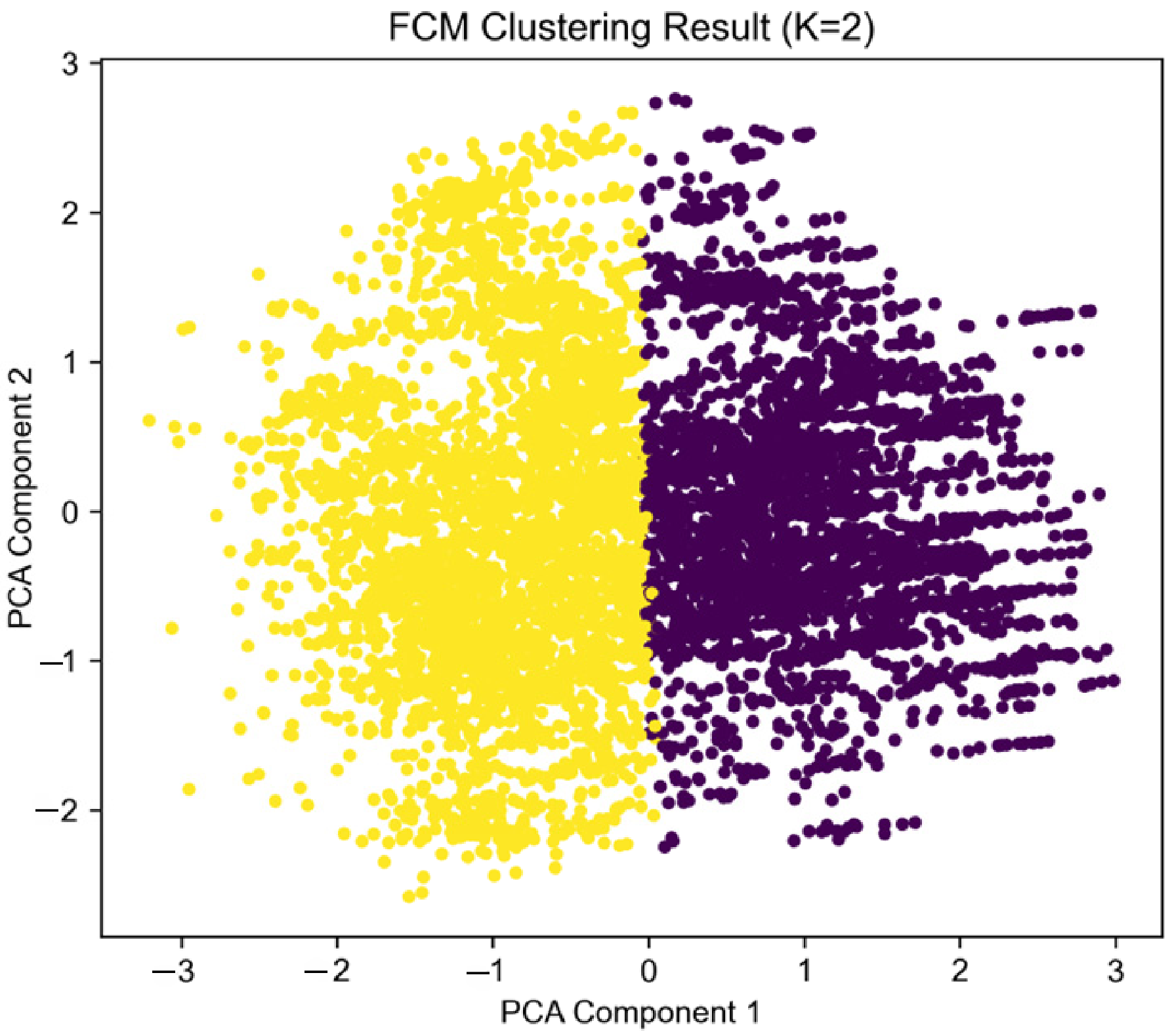
Since the input features are three-dimensional, PCA is implemented to compress the data to a two-dimensional space for a more intuitive visualization of the clustering results. The obtained clusters are shown in Figure 9:

Each point in the figure represents a wind power operating sample, while different colors indicate different clustering categories. As shown in the figure, the data exhibit a clear separation along the PCA1 dimension. The two wind condition categories form a distinct left–right distribution pattern, and the clustering boundary is relatively well defined. From the results, we can see that the FCM algorithm can reliably distinguish different wind condition states, indicating that the clustering outcome is primarily driven by wind velocity.

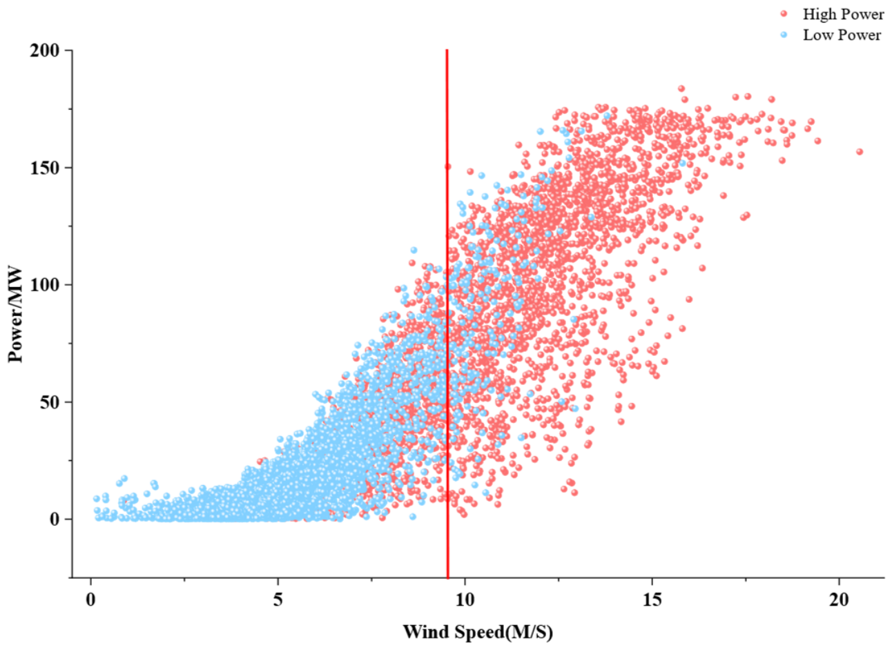
To further analyze the power output characteristics of wind turbines under different wind conditions, a scatter diagram of wind speed versus power output is generated, as presented in Figure 10:

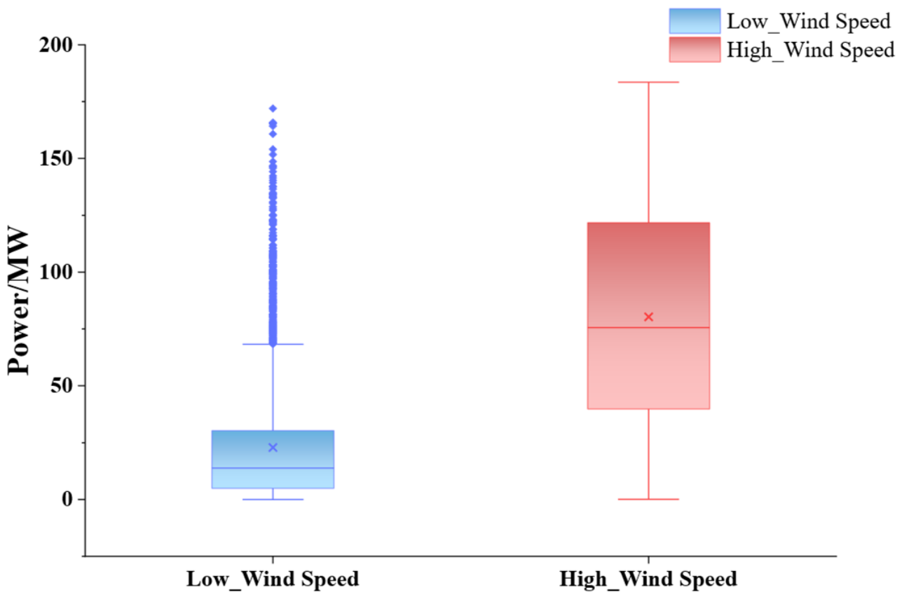
The power distribution characteristics of the two wind condition categories are illustrated in Figure 11.

As shown in the figure, the median power output under low-wind-speed conditions is relatively low, with most samples concentrated in the range of 0–30 MW, indicating that the overall wind turbines’ energy yield is low when wind speeds are low. For cases with low wind speeds, the median power output increases significantly, and the power distribution becomes much wider, with the maximum power approaching 180 MW, indicating that the turbines operate in a high-power region in scenarios with high wind velocity.

In this study, power forecasting is conducted separately for low-wind-speed and elevated wind speed operating situations. The outcomes are presented in terms of predicted curves and prediction errors for 12 h, 24 h, and 72 h forecasting horizons. Meanwhile, to ratify the superiority of the designed hybrid TCN–Transformer approach aimed at wind power prediction, several benchmark models, including TCN, LSTM, Transformer, and TCN–Transformer, are employed for comparative analysis under the same data conditions.

The dataset was divided into training and testing subsets using a chronological split strategy, where the first 80% of samples were used for training and the remaining 20% were reserved for testing. Temporal order was strictly preserved throughout the experiment to avoid information leakage.

All forecasting models were implemented in Python (version 3.9) using the PyTorch (version 2.6.0+cu124) framework. The Adam optimizer was employed for parameter optimization, and the mean squared error (MSE) was adopted as the loss function. The batch size was set to 64 and all models were trained for 100 epochs. ReLU activation was used in the TCN modules, while the Transformer encoder adopted the default GELU activation function provided by PyTorch.

To ensure a fair comparison, all benchmark models used the same input variables, sequence length, training/testing split strategy, batch size, optimizer, and loss function. Model-specific hyperparameters were selected according to commonly adopted settings in previous studies and preliminary experiments. The detailed hyperparameter settings are summarized in

Table 2. Hyperparameter settings of different forecasting models.

Hyperparameter	LSTM	GRU	BiGRU	Transformer	TCN	TCN–Transformer
Input features	4	4	4	4	4	4
Input sequence length	96	96	96	96	96	96
Output dimension	1	1	1	1	1	1
Hidden units	64	64	64 × 2	–	–	–
Number of recurrent layers	1	2	2	–	–	–
TCN channels	–	–	–	–	[32, 32, 64]	[32, 32, 64]
Kernel size	–	–	–	–	3	3
Dilation factors	–	–	–	–	[1, 2, 4]	[1, 2, 4]
Transformer encoder layers	–	–	–	2	–	2
Attention heads	–	–	–	4	–	4
Feed-forward dimension	–	–	–	256	–	256
Dropout	–	–	–	0.3	0.3	0.3
Optimizer	Adam	Adam	Adam	Adam	Adam	Adam
Learning rate	0.0001	0.0001	0.0001	0.0001	0.0001	0.0001
Batch size	64	64	64	64	64	64
Epochs	100	100	100	100	100	100
Loss function	MSE	MSE	MSE	MSE	MSE	MSE

.

All experiments were conducted on a workstation equipped with an Intel^® Core™ Ultra 9 185H CPU, 64 GB DDR5 RAM, and an NVIDIA GeForce RTX 4050 Laptop GPU. The proposed models were implemented using Python and PyTorch with CUDA acceleration.

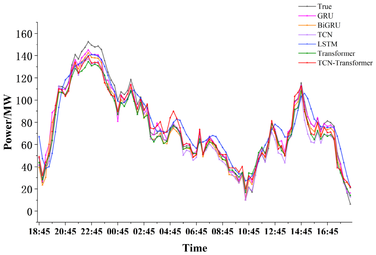
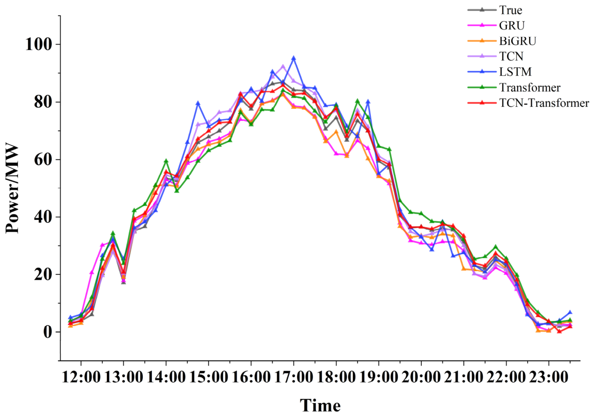
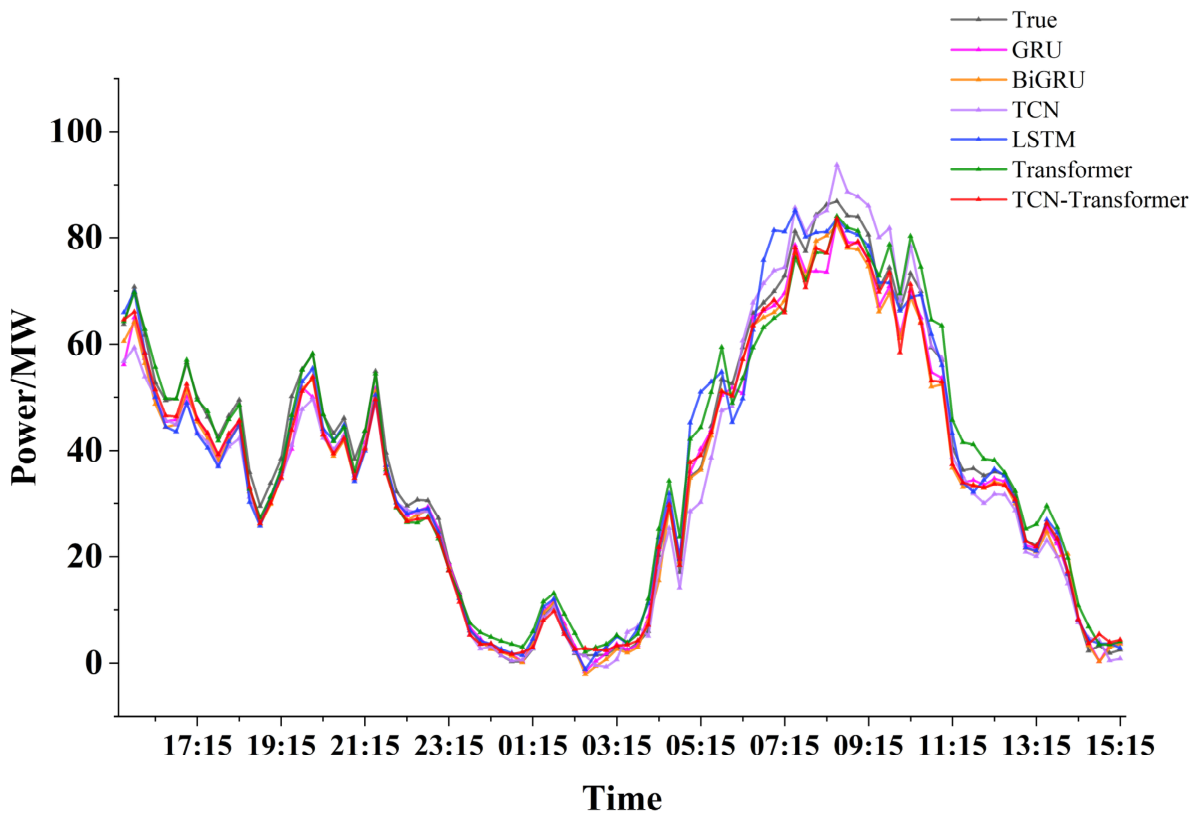
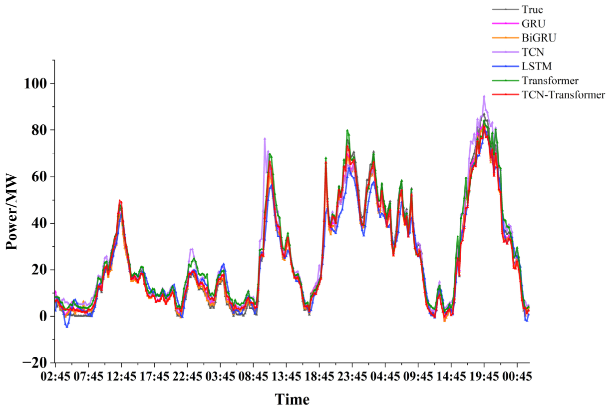
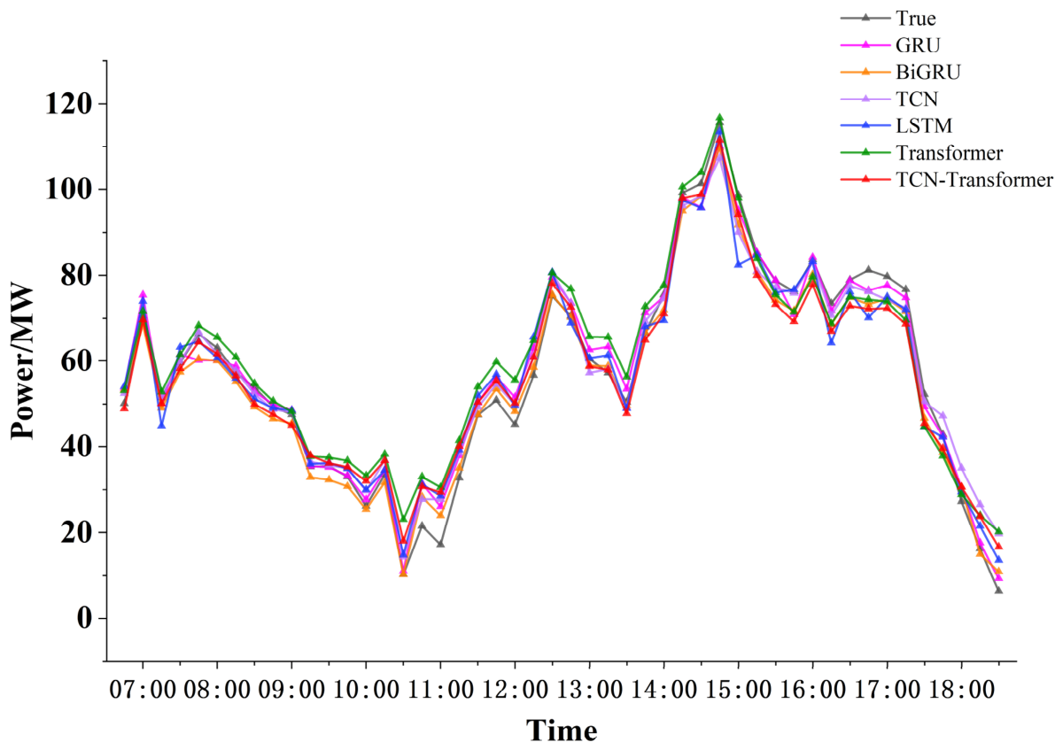
Figure 12, Figure 13 and Figure 14 show the multi-scale power forecasting results for cases where wind speed is low:

As shown in Figure 12, all models are generally able to capture the overall variation trend of wind power under low-wind-speed conditions. However, noticeable deviations can be observed near local peaks and valleys. Compared with the benchmark models, the proposed TCN–Transformer model follows the actual power curve more closely and exhibits smaller prediction errors during rapid power fluctuations. This result indicates that the hybrid architecture can effectively capture both short-term dynamic changes and long-range temporal dependencies, leading to more accurate short-term forecasting.

Figure 13 illustrates the forecasting results for the 24 h prediction horizon under low-wind-speed conditions. As the forecasting horizon increases, the prediction errors of all models become larger. Nevertheless, the proposed TCN–Transformer model still maintains good agreement with the actual power curve and provides more accurate predictions at several local extrema. The superior tracking performance demonstrates the effectiveness of combining TCN and Transformer for modeling complex wind power dynamics.

Figure 14 presents the forecasting results for the 72 h prediction horizon. Due to the longer forecasting horizon, the uncertainty of wind power increases significantly, resulting in larger deviations for all models. Despite this challenge, the proposed model remains capable of capturing the overall trend and major fluctuation patterns of the wind power series. The prediction curve generated by TCN–Transformer is generally closer to the actual observations than those of the competing models, confirming its strong long-term forecasting capability. Figure 15, Figure 16 and Figure 17 show the multi-scale power forecasting results during low wind velocity periods.

Figure 15 shows the forecasting performance under high-wind-speed conditions for the 12 h horizon. The proposed TCN–Transformer model accurately tracks the actual power variation and exhibits smaller deviations around both rising and falling periods. In contrast, several benchmark models tend to underestimate or overestimate power values near local peaks. These results demonstrate the ability of the proposed model to effectively characterize nonlinear power fluctuations under high-wind-speed operating conditions.

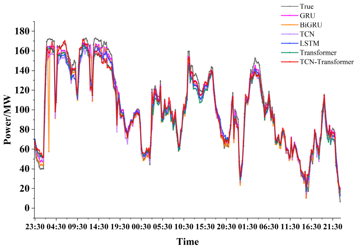
As illustrated in Figure 16, the forecasting task becomes more challenging under high-wind-speed conditions due to stronger power variability. Although all models capture the general trend of the power sequence, the proposed TCN–Transformer model achieves better consistency with the actual observations, particularly around rapid fluctuation intervals. This indicates that the hybrid framework can effectively improve forecasting accuracy by simultaneously exploiting local temporal features and long-range dependencies.

Figure 17 presents the most challenging forecasting scenario, namely 72 h ahead prediction under high-wind-speed conditions. The actual power series exhibits frequent fluctuations and several abrupt changes. Even under these complex conditions, the proposed TCN–Transformer model remains capable of reproducing the major variation trends and maintains relatively small prediction deviations. Compared with the benchmark models, its prediction curve shows better alignment with the actual power trajectory, further demonstrating the robustness and generalization ability of the proposed approach.

4. Discussion

To mitigate the influence of random initialization, all models were trained and evaluated five times using different random seeds (42, 52, 62, 72, 82). The following tables report the mean values of the evaluation metrics over these five independent runs.

Table 3. Error evaluation metrics under the condition of low wind speed.

Model	NMAE/% ± Std			NRMSE/% ± Std
	12 h	24 h	72 h	12 h	24 h	72 h
TCN	6.216 ± 0.003	5.939 ± 0.002	4.878 ± 0.003	7.919 ± 0.003	7.594 ± 0.002	6.680 ± 0.003
LSTM	6.593 ± 0.004	6.299 ± 0.002	5.182 ± 0.001	7.939 ± 0.004	7.801 ± 0.003	7.018 ± 0.002
GRU	6.544 ± 0.007	6.045 ± 0.004	4.623 ± 0.002	8.190 ± 0.007	7.674 ± 0.005	6.525 ± 0.004
BiGRU	6.061 ± 0.002	5.858 ± 0.001	5.246 ± 0.003	7.711 ± 0.002	7.366 ± 0.001	7.605 ± 0.002
Transformer	7.161 ± 0.007	6.779 ± 0.005	5.196 ± 0.002	8.852 ± 0.008	8.473 ± 0.006	6.780 ± 0.002
TCN–Transformer	5.213 ± 0.007	5.103 ± 0.013	4.003 ± 0.008	6.324 ± 0.010	6.437 ± 0.016	5.673 ± 0.011

shows the NMAE and NRMSE under low-wind-speed conditions:

Table 3 presents the forecasting performance of different models under low-wind-speed conditions based on five independent runs with different random seeds. The results are reported as mean ± standard deviation, providing a quantitative evaluation of both prediction accuracy and model robustness.

As shown in Table 3, the proposed TCN–Transformer model consistently achieves the best forecasting performance across all prediction horizons. Specifically, for the 12 h forecasting horizon, the proposed model obtains an NMAE of 5.213% and an NRMSE of 6.324%, which are lower than those of all benchmark models. Similar improvements can be observed for the 24 h and 72 h forecasting horizons, where the proposed model achieves the lowest NMAE and NRMSE values, demonstrating its superior capability in modeling complex wind power dynamics under low-wind-speed conditions.

Compared with the individual TCN and Transformer models, the superior performance of TCN–Transformer indicates that the two modules provide complementary advantages. The TCN component effectively extracts local temporal features through dilated causal convolutions, while the Transformer encoder captures long-range temporal dependencies via the self-attention mechanism. By combining these two mechanisms, the proposed model is able to learn more representative spatiotemporal features and achieve higher forecasting accuracy.

In addition to prediction accuracy, the standard deviation values of the proposed model remain very small across repeated runs. For example, the standard deviations of NMAE are only 0.007, 0.013, and 0.008 for the 12 h, 24 h, and 72 h forecasting horizons, respectively, while the corresponding standard deviations of NRMSE are 0.010, 0.016, and 0.011. These small deviations indicate that the proposed model is insensitive to random initialization and maintains stable forecasting performance across different runs, demonstrating strong robustness and reliability.

Furthermore, although forecasting uncertainty generally increases with the prediction horizon, the proposed TCN–Transformer model consistently preserves its performance advantage over all competing methods. This demonstrates that the hybrid architecture can effectively capture both short-term temporal patterns and long-range dependencies, resulting in accurate and stable wind power forecasting under low-wind-speed operating conditions.

Similarly,

Table 4. Error evaluation metrics under high-wind-speed conditions.

Model	NMAE/% ± Std			NRMSE/% ± Std
	12 h	24 h	72 h	12 h	24 h	72 h
TCN	8.014 ± 0.001	5.924 ± 0.003	5.804 ± 0.003	10.028 ± 0.001	7.383 ± 0.004	7.915 ± 0.003
LSTM	8.032 ± 0.002	6.291 ± 0.003	6.411 ± 0.004	9.695 ± 0.002	7.775 ± 0.004	8.591 ± 0.004
GRU	7.835 ± 0.002	5.401 ± 0.001	5.197 ± 0.002	9.522 ± 0.002	6.770 ± 0.001	7.493 ± 0.002
BiGRU	7.526 ± 0.001	5.428 ± 0.002	5.246 ± 0.003	9.212 ± 0.001	6.800 ± 0.002	7.605 ± 0.002
Transformer	7.924 ± 0.002	6.295 ± 0.006	5.516 ± 0.004	9.495 ± 0.003	7.750 ± 0.007	7.694 ± 0.003
TCN–Transformer	6.367 ± 0.008	4.963 ± 0.007	4.377 ± 0.004	8.434 ± 0.010	6.015 ± 0.007	6.212 ± 0.004

presents the mean NMAE and NRMSE over five repeated runs under high-wind-speed conditions:

Table 4 presents the forecasting performance of different models under high-wind-speed conditions based on five independent runs with different random seeds. The results are reported as mean ± standard deviation, allowing both prediction accuracy and robustness to be evaluated simultaneously.

As shown in Table 4, the proposed TCN–Transformer model consistently achieves the best forecasting performance across all prediction horizons. Specifically, for the 12 h forecasting horizon, the proposed model obtains an NMAE of 6.367% and an NRMSE of 8.434%, outperforming all benchmark models. Similar superiority can be observed for the 24 h and 72 h forecasting horizons, where the proposed model achieves the lowest NMAE and NRMSE values of 4.963%/6.015% and 4.377%/6.212%, respectively. These results demonstrate that the proposed hybrid architecture is capable of accurately capturing the complex nonlinear characteristics of wind power under high-wind-speed operating conditions.

Compared with the individual TCN and Transformer models, the TCN–Transformer model achieves noticeable performance improvements at all forecasting horizons. This indicates that the local temporal feature extraction capability of TCN and the long-range dependency modeling capability of Transformer are complementary. By integrating these two components, the proposed model can learn more representative temporal features and provide more accurate wind power forecasts.

The repeated experimental results also demonstrate the robustness of the proposed model. The standard deviations of NMAE are only 0.008, 0.007, and 0.004 for the 12 h, 24 h, and 72 h forecasting horizons, respectively, while the corresponding standard deviations of NRMSE are 0.010, 0.007, and 0.004. Such small fluctuations indicate that the proposed model is relatively insensitive to random initialization and can maintain stable forecasting performance across different runs.

Furthermore, it can be observed that recurrent neural network models (GRU and BiGRU) generally outperform the conventional LSTM model under high-wind-speed conditions, suggesting that gated recurrent structures are more effective in capturing dynamic variations in wind power series. Nevertheless, the proposed TCN–Transformer model consistently achieves the best overall performance, confirming the effectiveness of combining convolutional temporal feature extraction with self-attention-based global dependency learning for wind power forecasting.

Table 5. Average training time (mean ± standard deviation) of different models under low-wind-speed conditions for 24 h ahead forecasting.

Model	Average Training Time (s)	Std (s)
LSTM	9.442	0.351
GRU	10.068	0.744
BiGRU	12.767	0.598
Transformer	33.797	2.973
TCN	24.656	2.227
TCN–Transformer	59.845	4.164

presents the average training time and standard deviation of different forecasting models under low-wind-speed conditions for 24 h ahead forecasting. As shown, recurrent neural network-based models exhibit the lowest computational cost, with LSTM and GRU requiring only 9.442 s and 10.068 s on average, respectively. BiGRU slightly increases the training time to 12.767 s due to its bidirectional architecture.

Compared with recurrent models, Transformer-based approaches require more computational resources because of the self-attention mechanism. The Transformer model requires an average training time of 33.797 s, while the TCN model requires 24.656 s. The proposed TCN–Transformer model shows the highest computational cost, with an average training time of 59.845 s. This increase is expected because the model simultaneously incorporates temporal convolution operations and self-attention mechanisms to capture both local temporal patterns and long-range dependencies.

Nevertheless, considering the significant improvement in forecasting accuracy reported in Table 5, the additional computational cost remains acceptable. Furthermore, the standard deviations of all models are relatively small, indicating stable computational performance across repeated runs. Therefore, the proposed TCN–Transformer model achieves a favorable trade-off between forecasting accuracy and computational efficiency.

Although the proposed model requires longer training time than the benchmark models, the total training time remains within one minute on the experimental platform, demonstrating its practical applicability for short-term wind power forecasting tasks.

Table 6. Coefficient of determination (R²) under low-wind-speed conditions.

Model	12 h	24 h	72 h
TCN	0.936 ± 0.004	0.934 ± 0.004	0.939 ± 0.005
LSTM	0.936 ± 0.006	0.930 ± 0.005	0.933 ± 0.003
GRU	0.932 ± 0.110	0.932 ± 0.009	0.905 ± 0.026
BiGRU	0.939 ± 0.003	0.938 ± 0.002	0.904 ± 0.006
Transformer	0.920 ± 0.014	0.917 ± 0.011	0.938 ± 0.004
TCN–Transformer	0.943 ± 0.007	0.950 ± 0.006	0.942 ± 0.007

reports the coefficient of determination (R²) values obtained from five independent runs under low-wind-speed conditions. The results are presented as mean ± standard deviation to evaluate both the goodness of fit and the robustness of different forecasting models.

As shown in Table 6, all models achieve relatively high R² values above 0.90, indicating that they can effectively capture the variation trend of wind power under low-wind-speed conditions. Among all models, the proposed TCN–Transformer achieves the highest R² values at the 12 h, 24 h, and 72 h forecasting horizons, reaching 0.943, 0.950, and 0.942, respectively. These results demonstrate that the proposed hybrid architecture provides the best fitting performance and explains the largest proportion of variance in the actual wind power series.

Compared with the individual TCN and Transformer models, the superior R² values achieved by TCN–Transformer further confirm the complementary advantages of local feature extraction and long-range dependency modeling. The TCN module effectively captures short-term temporal patterns, while the Transformer encoder enhances the model’s ability to learn global contextual information. Their integration enables a more accurate representation of complex wind power dynamics.

In addition, the proposed model exhibits stable performance across repeated runs, with standard deviations of only 0.007, 0.006, and 0.007 for the 12 h, 24 h, and 72 h forecasting horizons, respectively. Such small fluctuations indicate that the model is insensitive to random initialization and maintains consistent forecasting performance.

It is also worth noting that the recurrent neural network models (LSTM, GRU, and BiGRU) generally achieve competitive R² values, whereas the standalone Transformer shows relatively lower fitting performance at the 12 h and 24 h horizons. Nevertheless, the proposed TCN–Transformer consistently achieves the highest R² values across all forecasting horizons, further validating the effectiveness and robustness of the proposed hybrid forecasting framework.

Table 7. Coefficient of determination (R²) under high-wind-speed conditions.

Model	12 h	24 h	72 h
TCN	0.797 ± 0.006	0.905 ± 0.010	0.896 ± 0.009
LSTM	0.810 ± 0.007	0.894 ± 0.010	0.878 ± 0.012
GRU	0.817 ± 0.008	0.884 ± 0.019	0.907 ± 0.004
BiGRU	0.768 ± 0.042	0.919 ± 0.005	0.904 ± 0.006
Transformer	0.818 ± 0.010	0.894 ± 0.021	0.902 ± 0.007
TCN–Transformer	0.828 ± 0.003	0.925 ± 0.002	0.923 ± 0.005

reports the R² values obtained from five independent runs under high-wind-speed conditions. The results are expressed as mean ± standard deviation to evaluate both the fitting accuracy and the stability of different forecasting models.

As shown in Table 7, all models achieve satisfactory fitting performance under high-wind-speed conditions, with most R² values exceeding 0.80. Among all compared models, the proposed TCN–Transformer consistently achieves the highest R² values across all forecasting horizons, reaching 0.828, 0.925, and 0.923 for the 12 h, 24 h, and 72 h forecasting tasks, respectively. These results indicate that the proposed model can explain a larger proportion of the variance in wind power data and provide more accurate forecasts under complex operating conditions.

Compared with the individual TCN and Transformer models, the superior performance of the TCN–Transformer model further demonstrates the effectiveness of combining local temporal feature extraction and global dependency learning. The TCN module captures short-term fluctuation patterns through dilated causal convolutions, while the Transformer encoder effectively models long-range temporal dependencies using the self-attention mechanism. Their integration enables the proposed model to better characterize the nonlinear dynamics of wind power generation.

The repeated experimental results also verify the robustness of the proposed model. The standard deviations of the R² values are only 0.003, 0.002, and 0.005 for the 12 h, 24 h, and 72 h forecasting horizons, respectively, which are among the lowest values observed across all models. Such small variations indicate that the proposed model is less sensitive to random initialization and can maintain stable forecasting performance over multiple independent runs.

It is also noteworthy that some recurrent neural network models exhibit relatively larger fluctuations under high-wind-speed conditions. For example, the BiGRU model achieves an R² of 0.768 ± 0.042 at the 12 h forecasting horizon, indicating greater sensitivity to random initialization and reduced stability. In contrast, the proposed TCN–Transformer model not only achieves the highest fitting accuracy but also maintains excellent consistency across repeated experiments. These findings further confirm the effectiveness and reliability of the proposed hybrid forecasting framework for wind power prediction under high-wind-speed conditions. To further evaluate the contribution of the FCM clustering strategy, an ablation experiment was conducted by comparing the proposed FCM–TCN–Transformer framework with a TCN–Transformer model trained directly on the original dataset without wind regime classification.

For a fair comparison, the forecasting results of the non-clustering TCN–Transformer model were separately evaluated under low-wind-speed and high-wind-speed conditions using the same wind regime labels obtained from the FCM clustering process. The prediction errors were then compared with those of the proposed framework.

Table 8. Ablation study of the FCM clustering strategy under low-wind-speed and high-wind-speed conditions.

Model	Low-Wind NMAE%	High-Wind NMAE%	Low-Wind NRMSE%	High-Wind NRMSE%
TCN–Transformer	7.592	6.087	8.664	8.021
FCM-TCN–Transformer	5.103	4.963	6.437	6.015

presents the forecasting performance of the TCN–Transformer model with and without FCM-based wind regime classification under low-wind-speed and high-wind-speed conditions.

As shown in Table 8, the proposed FCM–TCN–Transformer framework achieves consistently lower prediction errors under both operating conditions. Under low-wind-speed conditions, the NMAE decreases from 7.592% to 5.103%, corresponding to a reduction of 32.78%, while the NRMSE decreases from 8.664% to 6.437%, representing an improvement of 25.70%. Similarly, under high-wind-speed conditions, the NMAE is reduced from 6.087% to 4.963%, and the NRMSE decreases from 8.021% to 6.015%.

These results demonstrate that FCM clustering effectively partitions wind power data into more homogeneous operating regimes, thereby reducing data heterogeneity and facilitating more accurate forecasting. Consequently, the forecasting model can learn more representative features within each operating condition and achieve improved prediction accuracy.

Therefore, the improvement in the performance of the proposed framework can be attributed to two complementary factors. On the one hand, the hybrid TCN–Transformer architecture enhances forecasting accuracy by jointly capturing local temporal patterns and long-range temporal dependencies. On the other hand, the FCM clustering strategy improves data consistency by separating different operating conditions, allowing the forecasting model to learn more representative features within each wind regime. The combined effect of these two components ultimately leads to superior forecasting performance.

5. Conclusions

Accurate wind power forecasting is of great importance for improving renewable energy utilization and maintaining power system stability. To address the challenges caused by data heterogeneity, strong fluctuations, and complex temporal dependencies in wind power series, this study proposed a hybrid forecasting framework integrating FCM-based operating condition classification and a TCN–Transformer prediction model.

First, the FCM algorithm was employed to partition wind power data into low-wind-speed and high-wind-speed operating conditions, thereby reducing data heterogeneity and enabling more targeted modeling. Subsequently, a hybrid TCN–Transformer architecture was developed, in which the TCN module was responsible for extracting local temporal features, while the Transformer encoder captured long-range temporal dependencies through the self-attention mechanism. The proposed framework was evaluated using real SCADA data collected from a wind farm in Gansu Province, China.

The experimental results demonstrated that the proposed method consistently achieved the best forecasting performance under both low-wind-speed and high-wind-speed conditions. Across the 12 h, 24 h, and 72 h forecasting horizons, the TCN–Transformer model obtained lower NMAE and NRMSE values and higher R² values than the benchmark models, including LSTM, GRU, BiGRU, Transformer, and TCN. Furthermore, repeated experiments with different random seeds showed very small standard deviations, confirming the robustness and stability of the proposed approach.

From a practical perspective, the proposed framework can provide more reliable wind power forecasts under different operating conditions, thereby supporting wind farm operation management, power system dispatching, reserve scheduling, and renewable energy integration. By reducing forecasting uncertainty, the proposed method can contribute to improving the operational reliability and economic efficiency of modern power systems.

In terms of computational efficiency, the proposed TCN–Transformer model requires a higher computational cost than individual forecasting models because it combines both convolutional feature extraction and self-attention mechanisms. Nevertheless, the average training time remains less than one minute under the experimental settings, indicating that the model is computationally affordable for practical offline training applications. Considering the consistent improvement in forecasting accuracy, the additional computational cost is justified.

Despite the promising results, several limitations still exist. First, the proposed framework was validated using data from a single wind farm, and its generalization capability across different geographical regions remains to be further investigated. Second, only two operating conditions obtained through FCM clustering were considered in this study, while more refined condition classification strategies may further improve forecasting performance. Third, the forecasting framework relies primarily on historical SCADA variables and does not incorporate external numerical weather prediction (NWP) information. Future research will focus on multi-site validation, adaptive clustering strategies, and the integration of additional meteorological information to further enhance forecasting accuracy, robustness, and generalization capability.

References

1. Elmore, J.; Pearson, L. Considerations for cottonseed oil as a potential feedstock for renewable diesel production. Energy Rep. 2025, 13, 4072–4086. [Google Scholar] [CrossRef] [Scilit]
2. Li, F.; Wang, H.; Wang, D.; Liu, D.; Sun, K. A review of wind power prediction methods based on multi-time scales. Energies 2025, 18, 1713. [Google Scholar] [CrossRef] [Scilit]
3. Eikeland, E.F.; Hovem, F.D.; Olsen, T.E.; Chiesa, M.; Bianchi, F.M. Probabilistic forecasts of wind power generation in regions with complex topography using deep learning methods: An Arctic case. Energy Convers. Manag. X 2022, 15, 100239. [Google Scholar] [CrossRef] [Scilit]
4. Chen, Y.; Liu, J.; Yu, D. Economically-driven spatiotemporal collaborative correction of high-precision wind power forecasting curves: Aiming to more practical scheduling. Energy 2025, 337, 138678. [Google Scholar] [CrossRef] [Scilit]
5. Yang, Y.; Lou, H.; Wu, J.; Zhang, S.; Gao, S. A survey on wind power forecasting with machine learning approaches. Neural Comput. Appl. 2024, 36, 12753–12773. [Google Scholar] [CrossRef] [Scilit]
6. Haq, I.U.; Kumar, A.; Rathore, P.S. Machine learning approaches for wind power forecasting: A comprehensive review. Discov. Appl. Sci. 2025, 7, 1139. [Google Scholar] [CrossRef] [Scilit]
7. Sun, Y.; Han, W. A review of enhancing wind power with AI: Applications, economic implications, and green innovations. Digit. Econ. Sustain. Dev. 2025, 3, 11. [Google Scholar] [CrossRef] [Scilit]
8. Depuru, S.S.S.R.; Wang, L.; Devabhaktuni, V.; Gudi, N. Measures and Setbacks for Controlling Electricity Theft. In Proceedings of the North American Power Symposium 2010, Arlington, TX, USA, 26–28 September 2010; IEEE: Piscataway, NJ, USA, 2010; pp. 1–8. [Google Scholar] [CrossRef] [Scilit]
9. Wu, J.; Wang, Z.-X.; Wang, G.-Q. The key technologies and development of offshore wind farm in China. Renew. Sustain. Energy Rev. 2014, 34, 453–462. [Google Scholar] [CrossRef] [Scilit]
10. Foley, A.M.; Leahy, P.G.; Marvuglia, A.; McKeogh, E.J. Current methods and advances in forecasting of wind power generation. Renew. Energy 2012, 37, 1–8. [Google Scholar] [CrossRef] [Scilit]
11. Santhosh, M.; Venkaiah, C.; Vinod Kumar, D.M. Current advances and approaches in wind speed and wind power forecasting for improved renewable energy integration: A review. Eng. Rep. 2020, 2, e12178. [Google Scholar] [CrossRef] [Scilit]
12. Hossain, M.A.; Chakrabortty, R.K.; Elsawah, S.; Ryan, M.J. Very short-term forecasting of wind power generation using hybrid deep learning model. J. Clean. Prod. 2021, 296, 126564. [Google Scholar] [CrossRef] [Scilit]
13. Phan, Q.T.; Wu, Y.K.; Phan, Q.D. A Hybrid Wind Power Forecasting Model with XGBoost, Data Preprocessing Considering Different NWPs. Appl. Sci. 2021, 11, 1100. [Google Scholar] [CrossRef] [Scilit]
14. Yu, R.; Gao, J.; Yu, M.; Lu, W.; Xu, T.; Zhao, M.; Zhang, J.; Zhang, R.; Zhang, Z. LSTM-EFG for wind power forecasting based on sequential correlation features. Future Gener. Comput. Syst. 2019, 93, 33–42. [Google Scholar] [CrossRef] [Scilit]
15. Hossain, M.A.; Gray, E.; Lu, J.; Islam, R.; Alam, S.; Chakrabortty, R.; Pota, H.R. Optimized Forecasting Model to Improve the Accuracy of Very Short-Term Wind Power Prediction. IEEE Trans. Ind. Inform. 2023, 19, 10145–10159. [Google Scholar] [CrossRef] [Scilit]
16. Shao, Z.; Han, J.; Zhao, W.; Zhou, K.; Yang, S. Hybrid model for short-term wind power forecasting based on singular spectrum analysis and a temporal convolutional attention network with an adaptive receptive field. Energy Convers. Manag. 2022, 269, 116138. [Google Scholar] [CrossRef] [Scilit]
17. Li, H.; Wang, J.; Lu, H.; Guo, Z. Research and application of a combined model based on variable weight for short term wind speed forecasting. Renew. Energy 2018, 116, 669–684. [Google Scholar] [CrossRef] [Scilit]
18. Ye, L.; Li, Y.; Pei, M.; Zhao, Y.; Li, Z.; Lu, P. A novel integrated method for short-term wind power forecasting based on fluctuation clustering and history matching. Appl. Energy 2022, 327, 120131. [Google Scholar] [CrossRef] [Scilit]
19. Zhang, C.; Wei, H.; Zhao, J.; Liu, T.; Zhu, T.; Zhang, K. Short-term wind speed forecasting using empirical mode decomposition and feature selection. Renew. Energy 2016, 96, 727–737. [Google Scholar] [CrossRef] [Scilit]
20. Pinson, P.; Nielsen, H.A.; Møller, J.K.; Madsen, H.; Kariniotakis, G.N. Non-parametric probabilistic forecasts of wind power: Required properties and evaluation. Wind Energy 2007, 10, 497–516. [Google Scholar] [CrossRef] [Scilit]
21. Khosravi, A.; Nahavandi, S.; Creighton, D.; Atiya, A.F. Comprehensive Review of Neural Network-Based Prediction Intervals and New Advances. IEEE Trans. Neural Netw. 2011, 22, 1341–1356. [Google Scholar] [CrossRef] [Scilit] [PubMed]
22. Rathod, D.; Gidwani, L. A literature review based on density forecasting and uncertainty quantification of wind power generation. Renew. Sustain. Energy Rev. 2026, 229, 116559. [Google Scholar] [CrossRef] [Scilit]
23. Alharthi, Y.Z.; Chiroma, H.; Gabralla, L.A. Enhanced framework embedded with data transformation and multi-objective feature selection algorithm for forecasting wind power. Sci. Rep. 2025, 15, 16119. [Google Scholar] [CrossRef] [Scilit] [PubMed]
24. Hua, H.; Wang, Y.; Han, K.; Liu, C.; Zhang, K.; Chen, P.; Bao, Y.; Mei, J. Power prediction method of the offshore wind farm considering high-dimensional feature selection and physical guidance. Electr. Power Syst. Res. 2026, 250, 112151. [Google Scholar] [CrossRef] [Scilit]
25. Khazaei, S.; Ehsan, M.; Soleymani, S.; Mohammadnezhad-Shourkaei, H. A high-accuracy hybrid method for short-term wind power forecasting. Energy 2022, 238, 122020. [Google Scholar] [CrossRef] [Scilit]
26. Sharma, K.B.; Jha, S.K.; Singh, S.K. Feature Selection Using Hybrid Machine Learning Approach for Wind Power Generation. In 2025 3rd International Conference on Communication, Security, and Artificial Intelligence (ICCSAI), Greater Noida, India, 4–6 April 2025; IEEE: Piscataway, NJ, USA, 2025; pp. 159–164. [Google Scholar] [CrossRef] [Scilit]
27. Isik, M.; Yalcinkaya, M. Integrated regime-aware wind power forecasting using multi-altitude meteorological features and hybrid machine learning. Front. Energy Res. 2026, 13, 1686125. [Google Scholar] [CrossRef] [Scilit]
28. Yuan, W.; Yang, H.; Han, Z.; Zhang, Y. Enhancing wind power forecasting accuracy under extreme weather: Leveraging a dual-model approach with condition-based classification. Eng. Appl. Artif. Intell. 2025, 162, 112656. [Google Scholar] [CrossRef] [Scilit]
29. Peng, D.; Liu, Y.; Wang, D.; Luo, L.; Zhao, H.; Qu, B. Short-term PV-Wind forecasting of large-scale regional site clusters based on FCM clustering and hybrid Inception-ResNet embedded with Informer. Energy Convers. Manag. 2024, 320, 118992. [Google Scholar] [CrossRef] [Scilit]
30. Zhou, B.; Ma, X.; Luo, Y.; Yang, D. Wind Power Prediction Based on LSTM Networks and Nonparametric Kernel Density Estimation. IEEE Access 2019, 7, 165279–165292. [Google Scholar] [CrossRef] [Scilit]
31. Villegas Pico, H.; McCalley, J.D.; Angel, A.; Leon, R.; Castrillon, N.J. Analysis of Very Low Frequency Oscillations in Hydro-Dominant Power Systems Using Multi-Unit Modeling. IEEE Trans. Power Syst. 2012, 27, 1906–1915. [Google Scholar] [CrossRef] [Scilit]
32. Babu, M.R.; Badar, A.Q.H.; Balasubramani, S. Fuzzy-C Means Clustering Based ANFIS wind speed forecast. In 2020 21st National Power Systems Conference (NPSC), Gandhinagar, India, 17–19 December 2020; IEEE: Piscataway, NJ, USA, 2020; pp. 1–6. [Google Scholar] [CrossRef] [Scilit]
33. Han, J.; Li, L.; Song, H.; Liu, M.; Song, Z.; Qu, Y. An Equivalent Model of Wind Farm Based on Multivariate Multi-Scale Entropy and Multi-View Clustering. Energies 2022, 15, 6054. [Google Scholar] [CrossRef] [Scilit]
34. Yang, Y.; Xu, Y.; Gu, W.; Mili, L.; Sun, B.; Lu, S.; Shen, C. A Tensor-Based Clustering Method for Dynamic Equivalent Modeling of Wind Farms. IEEE Trans. Sustain. Energy 2026, 17, 1075–1089. [Google Scholar] [CrossRef] [Scilit]
35. Wang, Y.; Zou, R.; Liu, F.; Zhang, L.; Liu, Q. A review of wind speed and wind power forecasting with deep neural networks. Appl. Energy 2021, 304, 117766. [Google Scholar] [CrossRef] [Scilit]
36. Krishnapuram, R.; Keller, J.M. A possibilistic approach to clustering. IEEE Trans. Fuzzy Syst. 1993, 1, 98–110. [Google Scholar] [CrossRef] [Scilit]
37. Pal, N.R.; Bezdek, J.C. On cluster validity for the fuzzy c-means model. IEEE Trans. Fuzzy Syst. 1995, 3, 370–379, Correction in IEEE Trans. Fuzzy Syst. 19975, 152–153. [Google Scholar] [CrossRef] [Scilit]
38. Song, R.; Huang, S.; Xiong, L.; Zhou, Y.; Li, T.; Tan, P.; Sun, Z. Takagi-Sugeno fuzzy parallel distributed compensation control for low-frequency oscillation suppression in wind energy-penetrated power systems. Electronics 2024, 13, 3795. [Google Scholar] [CrossRef] [Scilit]
39. Liu, L.; Hu, X.; Chen, J.; Wu, R.; Chen, F. Embedded Scenario Clustering for Wind and Photovoltaic Power, and Load Based on Multi-Head Self-Attention. Prot. Control Mod. Power Syst. 2024, 9, 122–132. [Google Scholar] [CrossRef] [Scilit]
40. Wang, K.; Qi, X.; Liu, H.; Song, J. Deep belief network based k-means cluster approach for short-term wind power forecasting. Energy 2018, 165, 840–852. [Google Scholar] [CrossRef] [Scilit]
41. Lin, X.; Meng, W.; Yu, M.; Luo, Q. Optimal Configuration Method for Offshore Wind Power Energy Storage Based on Improved Typical Day Clustering Algorithm. In 2025 2nd International Symposium on New Energy Technologies and Power Systems (NETPS), Hangzhou, China, 23–25 May 2025; IEEE: Piscataway, NJ, USA, 2025; pp. 81–85. [Google Scholar] [CrossRef] [Scilit]
42. Rubio, E.; Castillo, O.; Melin, P. A new Interval Type-2 Fuzzy Possibilistic C-Means clustering algorithm. In 2015 Annual Conference of the North American Fuzzy Information Processing Society (NAFIPS) held Jointly with 2015 5th World Conference on Soft Computing (WConSC), Redmond, WA, USA, 17–19 August 2015; IEEE: Piscataway, NJ, USA, 2015; pp. 1–5. [Google Scholar] [CrossRef] [Scilit]
43. Yang, H.; Shu, Z.; Li, Z. Enhanced wind power forecasting using a hybrid multi-strategy coati optimization algorithm and backpropagation neural network. Sensors 2025, 25, 2438. [Google Scholar] [CrossRef] [Scilit] [PubMed]
44. Liu, Y.; Song, K.; Fan, F.; Wang, Y.; Ge, M.; Sun, C. Short-Term Wind Power Forecasting Based on Adaptive LSTM and BP Neural Network. Appl. Sci. 2025, 15, 11244. [Google Scholar] [CrossRef] [Scilit]
45. Sarkar, M.R.; Anavatti, S.G.; Ferdaus, M.M.; Dam, T. ASPEN-WIND: Adaptive spectral and self-supervised interactive CNN-LSTM for enhanced wind power forecasting. Expert Syst. Appl. 2026, 296, 129171. [Google Scholar] [CrossRef] [Scilit]
46. Adekunle, A.; Fofana, I.; Picher, P.; Rodriguez-Celis, E.M.; Arroyo-Fernandez, O.H.; Zemouri, R. Optimizing deep learning predictive models: A comprehensive review of RNN and its variant architectures. Appl. Soft Comput. 2025, 185, 114015. [Google Scholar] [CrossRef] [Scilit]
47. Fan, J.; Yu, G.-A.; Zhao, M.; Zong, H. MCPT-CAF-BiGRU: A multi-scale CNN and ProbSparse-Masked Transformer model with cross-attention fusion and BiGRU for hourly wind speed forecasting. Expert Syst. Appl. 2026, 307, 131081. [Google Scholar] [CrossRef] [Scilit]
48. Cai, X.; Li, D.; Zou, Y.; Liu, Z.; Heidari, A.A.; Chen, H. A hybrid wind speed forecasting model with rolling mapping decomposition and temporal convolutional networks. Energy 2025, 324, 135673. [Google Scholar] [CrossRef] [Scilit]
49. Song, Z.; Gu, Y.; Liu, H.; Zou, T.; Lin, Y.; Ye, K. Application of deep learning in wind, solar, and ocean energy: An analysis of prediction, optimization, and operation & maintenance. Renew. Sustain. Energy Rev. 2026, 230, 116663. [Google Scholar] [CrossRef] [Scilit]
50. Chen, C.; Wan, H.; Peng, B.; Quan, R.; Chang, Y.; Derigent, W. Accurate multi-step wind and solar power forecasting based on multi-scale convolutional Kolmogorov-Arnold network and improved Lemming-optimized attention fusion. Eng. Appl. Artif. Intell. 2026, 163, 112832. [Google Scholar] [CrossRef] [Scilit]
51. Fan, H.; Shi, Y.; Fu, Z.; Chen, S.; Wei, W.; Xu, W.; Li, J. WindFM: An Open-Source Foundation Model for Zero-Shot Wind Power Forecasting. arXiv 2025, arXiv:2509.06311. [Google Scholar] [CrossRef] [Scilit]
52. Gao, Y.; Hu, S.; Chen, Y.; Khan, M.F.; Cheng, X.; Yang, J. A novel probabilistic wind power forecasting framework integrating similar curve matching mechanism and an enhanced conditional diffusion model. Appl. Energy 2026, 402, 127031. [Google Scholar] [CrossRef] [Scilit]
53. de la Rosa, L.R.; García-Pérez, L.; Peñas, M.S.; Gómez, A. Hybrid model to improve wind energy prediction considering data granularity. Results Eng. 2025, 28, 107646. [Google Scholar] [CrossRef] [Scilit]
54. Jia, W.; An, A.; Gong, B.; Shi, Y.; Yan, Z. A multi-variable driven dual-stage modal-decoupling framework integrating deterministic–uncertainty modeling for wind power forecasting with feature interpretability analysis. Energy 2026, 344, 139884. [Google Scholar] [CrossRef] [Scilit]
55. Yao, X.; Xu, H. A HybridGCN-GRU approach for high-accuracy wind speed forecasting via multi-graph feature fusion and dynamic modeling. Inf. Sci. 2026, 728, 122805. [Google Scholar] [CrossRef] [Scilit]
Figure 1. Scatter plot of raw wind speed (m/s) versus power output (MW) from the SCADA data before preprocessing. The figure was created using OriginPro 2026 (OriginLab Corporation, Northampton, MA, USA).
Inventions 11 00062 g001
Figure 2. Pearson correlation coefficients between five meteorological features (average wind speed, average wind direction, air pressure, temperature, humidity) and the actual wind power output.
Inventions 11 00062 g002
Figure 3. Schematic diagram of the Temporal Convolutional Network (TCN) architecture for time series forecasting.
Inventions 11 00062 g003
Figure 4. Workflow of Transformer model for time series forecasting, including encoder, decoder, multi-head attention, and feed-forward layers.
Inventions 11 00062 g004
Figure 5. Architecture of the proposed hybrid TCN–Transformer model. The input time series is first processed by a TCN module, which uses causal and dilated convolutions to extract local temporal features across multiple scales. The output of the TCN is then fed into a Transformer encoder, which applies multi-head self-attention to capture global dependencies among distant time steps. The combined features are finally passed through fully connected layers to produce the wind power prediction. This hybrid design leverages TCN’s strength in local feature extraction and Transformer’s strength in global dependency modeling.
Inventions 11 00062 g005
Figure 6. Complete flowchart of the proposed wind power forecasting method.
Inventions 11 00062 g006
Figure 7. Low-speed conditions.
Inventions 11 00062 g007
Figure 8. High-speed conditions.
Inventions 11 00062 g008
Figure 9. Principal component analysis (PCA) visualization of the FCM clustering results with C = 2 clusters. The original three-dimensional input features (wind speed, wind direction, air pressure) are projected onto the first two principal components (PCA1 and PCA2). Samples belonging to Cluster 1 (low wind speed) are shown in yellow on the left side of the plot, while samples belonging to Cluster 2 (high wind speed) are shown in purple on the right side. The two clusters are clearly separated along the PCA1 axis, indicating that wind speed is the dominant factor driving the clustering. The boundary between the clusters is well defined, with minimal overlap, demonstrating that FCM effectively distinguishes different wind operating conditions. This separation justifies the subsequent strategy of building separate prediction models for low- and high-wind-speed regimes.
Inventions 11 00062 g009
Figure 10. Wind speed versus power scatter plots for the two FCM clusters overlaid on the same axes. Blue points correspond to low-wind-speed regime (Cluster 1), and red points correspond to high-wind-speed regime (Cluster 2). The plot clearly shows that the low-speed regime is confined to wind speeds below 9 m/s with power below 30 MW, while the high-speed regime covers wind speeds from 9 to 20 m/s with power ranging from near zero up to 180 MW. The transition between the two regimes is smooth, reflecting the continuous nature of wind power generation. This separation justifies the use of condition-aware modeling. The vertical line at 9 m/s marks the boundary between the low- and high-wind-speed regimes identified by FCM clustering. As shown in the figure, the power generated by the wind turbine increases with wind velocity, exhibiting a clear nonlinear growth relationship, which is in agreement with the typical power curve properties of wind turbines. In Figure 10, the low-wind-speed samples are mainly distributed within the bounds of 0–9 m/s, where the power output is relatively low with small fluctuations. In contrast, the high-wind-speed samples are primarily distributed in the range of 9–20 m/s, where the power output increases significantly and gradually approaches the turbine’s rated output.
Inventions 11 00062 g010
Figure 11. Boxplot comparison of power output distributions for low (blue) and high (red) wind speed regimes. For the low-speed regime, the median power is approximately 5 MW, the interquartile range (IQR) is narrow (0–15 MW), and the maximum is about 30 MW. For the high-speed regime, the median power is around 80 MW, the IQR is wide (40–140 MW), and the maximum reaches 180 MW. The high-speed regime also shows more outliers, indicating higher variability. This figure quantitatively demonstrates that the two regimes have fundamentally different power characteristics, further supporting the need for separate modeling.
Inventions 11 00062 g011
Figure 12. Comparison of actual vs. predicted wind power under low-wind-speed conditions with a 12 h forecasting horizon. Actual power: black. Predicted: TCN (purple), LSTM (blue), Transformer (green), GRU (pink), BiGRU (orange), and proposed TCN–Transformer (red). The proposed model (red) achieves the closest tracking of the actual curve, outperforming all baselines.
Inventions 11 00062 g012
Figure 13. Comparison of actual vs. predicted wind power under low-wind-speed conditions with a 24 h forecasting horizon.
Inventions 11 00062 g013
Figure 14. Comparison of actual vs. predicted wind power under low-wind-speed condition with a 72 h forecasting horizon.
Inventions 11 00062 g014
Figure 15. Comparison of actual vs. predicted wind power under high-wind-speed conditions with a 12 h forecasting horizon.
Inventions 11 00062 g015
Figure 16. Comparison of actual vs. predicted wind power under high-wind-speed conditions with a 24 h forecasting horizon.
Inventions 11 00062 g016
Figure 17. Comparison of actual vs. predicted wind power under high-wind-speed conditions with a 72 h forecasting horizon.
Inventions 11 00062 g017