An Intelligent Computing Architecture for Ultra-Short-Term Wind Power Forecasting: Integrating Dual-Stage Signal Processing and Optimized Deep Learning

Abstract

The integration of wind energy into power systems relies on forecasting technologies to address operational challenges caused by its volatility and intermittency. This paper proposes a computing architecture for ultra-short-term wind power forecasting. The methodology integrates an adaptive dual-stage signal processing technique with an optimized deep learning model. To manage the non-stationarity of meteorological variables, the Pearson and Maximal Information Coefficient (MIC) analyses are employed for feature selection. The ICEEMDAN algorithm is then used for initial decomposition, followed by sample entropy and K-Means clustering to assess component complexity. Variational Mode Decomposition (VMD) is applied only to the high-frequency component to further separate stochastic fluctuations while preserving relatively stable trend components. A Convolutional Neural Network-Bidirectional Long Short-Term Memory (CNN-BiLSTM) network is constructed to forecast the resulting multi-scale components. To reduce reliance on manual empirical tuning, the Crested Porcupine Optimizer (CPO) is used to fine-tune key network hyperparameters. Evaluations using operational wind-farm data indicate that the developed hybrid method captures the temporal dynamics of wind power and yields lower prediction errors than the tested benchmark models. This research provides a data-driven computing framework for renewable-energy forecasting and related operational analysis.

1. Introduction

The profound restructuring of the global energy mix and the ever-increasing demand for clean energy have intensified the penetration of wind and photovoltaic power into the grid, transforming modern power systems into complex dynamic systems characterized by large-scale, high-proportion renewable energy integration [1,2]. While this accelerates the low-carbon energy transition, it also exacerbates the risks to stable grid operation stemming from the inherent strong volatility and intermittency of wind power output. The grid incident in Spain and Portugal on 28 April 2025 was documented by ENTSO-E as a large-scale blackout, and the final report identifies causes of the event and recommendations for strengthening the resilience of the interconnected European power system [3]. This incident exposed that, in power systems with high penetration of wind and solar energy, a lack of accurate forecasting and flexible dispatch under extreme conditions can lead to sudden changes in output that directly threaten grid security [4,5,6,7]. Power systems face operational pressures and potential risks due to wind power uncertainty; thus, developing effective countermeasures through accurate power forecasting to ensure stable operation has become an important task [8]. In congested transmission systems, chance-constrained scheduling of compressed-air energy storage and demand-response programs has also been used to support wind-power harvesting under operational flexibility requirements [9].

The inherent strong randomness and high volatility of wind power originate from the high sensitivity of its driving forces to meteorological conditions and geographical environments [10,11]. Uncovering the deep relationships between these data and wind power is key to improving forecasting accuracy. Currently, forecasting can be categorized by time scale into ultra-short-term, short-term, and medium-to-long-term; by principle, it can be divided into physical methods and statistical methods. Physical methods are typically used for medium-to-long-term forecasting and rely on solving multi-dimensional nonlinear partial differential equations to map numerical weather characteristics to the output power curves of wind turbines, which are then extrapolated into forecast series [12]. Although these methods can describe the physical process of wind energy conversion from a first-principles perspective, they have stringent requirements for modeling accuracy and low computational efficiency, failing to meet the timeliness demands of ultra-short-term forecasting. Statistical methods, on the other hand, focus more on learning underlying spatio-temporal evolution patterns from historical observation data [13]. Traditional methods such as Auto Regressive Moving Average (ARMA) [14], Kalman filtering [15] and Fourier transforms can construct predictive models using limited linear data. However, as wind power series themselves exhibit a high degree of uncertainty, the performance of these methods is severely constrained when fitting complex dynamic relationships. They often presuppose the linearity and stationarity of the data, which contradicts the actual conditions of typical wind power data containing noise, outliers, and abrupt changes, thereby leading to drawbacks such as low prediction accuracy and weak generalization ability [16].

With the rapid development of artificial intelligence technology, methods represented by deep learning have been applied to the field of ultra-short-term wind power forecasting and have become a mainstream research trend. Various neural network architectures, such as Recurrent Neural Networks (RNN) [17], Long Short-Term Memory (LSTM) [18], and Gate Recurrent Unit (GRU) [19], are widely used due to their ability to capture long-term dependencies in time-series data. Reference [20] applied LSTM to forecast wind power generation, validating its effectiveness for predicting highly random time-series data; however, its unidirectional information flow in the gating mechanism is prone to overfitting. To overcome this limitation, Bidirectional LSTM (BiLSTM) was proposed, which can more comprehensively understand the temporal dependencies of wind power by simultaneously processing forward and backward temporal information [21]. Furthermore, due to the advantages of Convolutional Neural Networks (CNN) in extracting local spatial features and one-dimensional sequence patterns, Reference [22] combined CNN with LSTM to enhance the model’s ability to learn meteorological temporal features in wind power data. Although these deep learning models have made significant progress in improving ultra-short-term forecasting accuracy, when faced with the inherent extreme complexity, multi-scale variability, and deep coupling characteristics of wind power time-series signals, single or simply combined models cannot fully excavate key dynamic information or capture the temporal patterns of nonlinear or drastically fluctuating data, leading to significantly reduced robustness and accuracy [23].

To further address the constraints imposed by wind power signal characteristics on the prediction accuracy and to enhance the quality of input data and prediction performance of deep learning models, signal decomposition techniques have been widely applied in the data preprocessing stage [24]. The core idea is to decompose the original complex wind power series into a series of relatively simple and stationary Intrinsic Mode Functions (IMFs) or sub-series, thereby reducing its volatility and nonlinearity [25]. Empirical Mode Decomposition (EMD), an early and widely used adaptive time-frequency analysis method [26], is susceptible to noise interference and may produce mode mixing problems when processing actual wind power signals, severely affecting the accuracy of subsequent processing. To overcome the shortcomings of EMD, improved variant algorithms such as Ensemble Empirical Mode Decomposition (EEMD) add Gaussian white noise multiple times to the original signal and average the IMF sets obtained from multiple EMDs, utilizing the zero-mean property of noise to smooth mode mixing [27]; however, the introduced auxiliary noise is difficult to completely eliminate. Furthermore, Complete Ensemble Empirical Mode Decomposition with Adaptive Noise (CEEMDAN) improves upon EEMD by adding specific adaptive noise during the decomposition phase and extracting IMFs after calculating the residuals, achieving better robustness and smaller reconstruction errors [28]. Additionally, Variational Mode Decomposition (VMD), as another mainstream technique, transforms signal decomposition into a constrained variational problem for optimization, exhibiting good anti-noise performance and mode separation accuracy. Reference [29] combined it with an improved LSTM to forecast multivariate mixed wind power data. However, single signal decomposition methods still have inherent limitations. For example, VMD is sensitive to the selection of parameters such as the number of modes and the penalty factor, lacks adaptability, and is prone to over-decomposition or under-decomposition issues when the signal-to-noise ratio is low and frequency domain aliasing occurs; after CEEMDAN decomposition, some high-frequency IMFs may still carry high complexity and residual noise. In view of this, dual-mode multi-level decomposition methods have been proposed to address the aforementioned problems. Reference [30] applied CEEMDAN and VMD in cascade to achieve finer signal decoupling. However, conventional cascade strategies apply secondary decomposition to all components unconditionally, which increases computational overhead and risks over-decomposing stable low-frequency trends. There is still a necessity to optimize combined decomposition strategies by selectively eliminating residual high-frequency noise while reducing information loss.

To address the deficiencies of existing wind power forecasting methods in handling highly nonlinear and non-stationary wind power series and in model optimization, this paper proposes an ultra-short-term wind power forecasting method based on a hybrid CPO (Crested Porcupine Optimizer)-ICEEMDAN-VMD-CNN-BiLSTM architecture. The method first preliminarily decomposes the original wind power series using the improved ICEEMDAN, classifies the IMF components using sample entropy and K-Means clustering, and performs a targeted VMD secondary decomposition specifically on the high-frequency complex components to extract multi-scale features. Then, the processed final components are input in parallel into the CNN-BiLSTM model, where CNN extracts local features, the BiLSTM captures bidirectional temporal dependencies, and the CPO algorithm performs optimization of the network’s hyperparameters. Using historical power data and meteorological data from an actual wind farm for case simulation, the experimental results show that the proposed method yields lower prediction errors compared to various benchmark models. The implementation flowchart of the CPO-ICEEMDAN-VMD-CNN-BiLSTM prediction model proposed in this paper is illustrated in Figure 1.

The main contributions of this paper are summarized as follows:

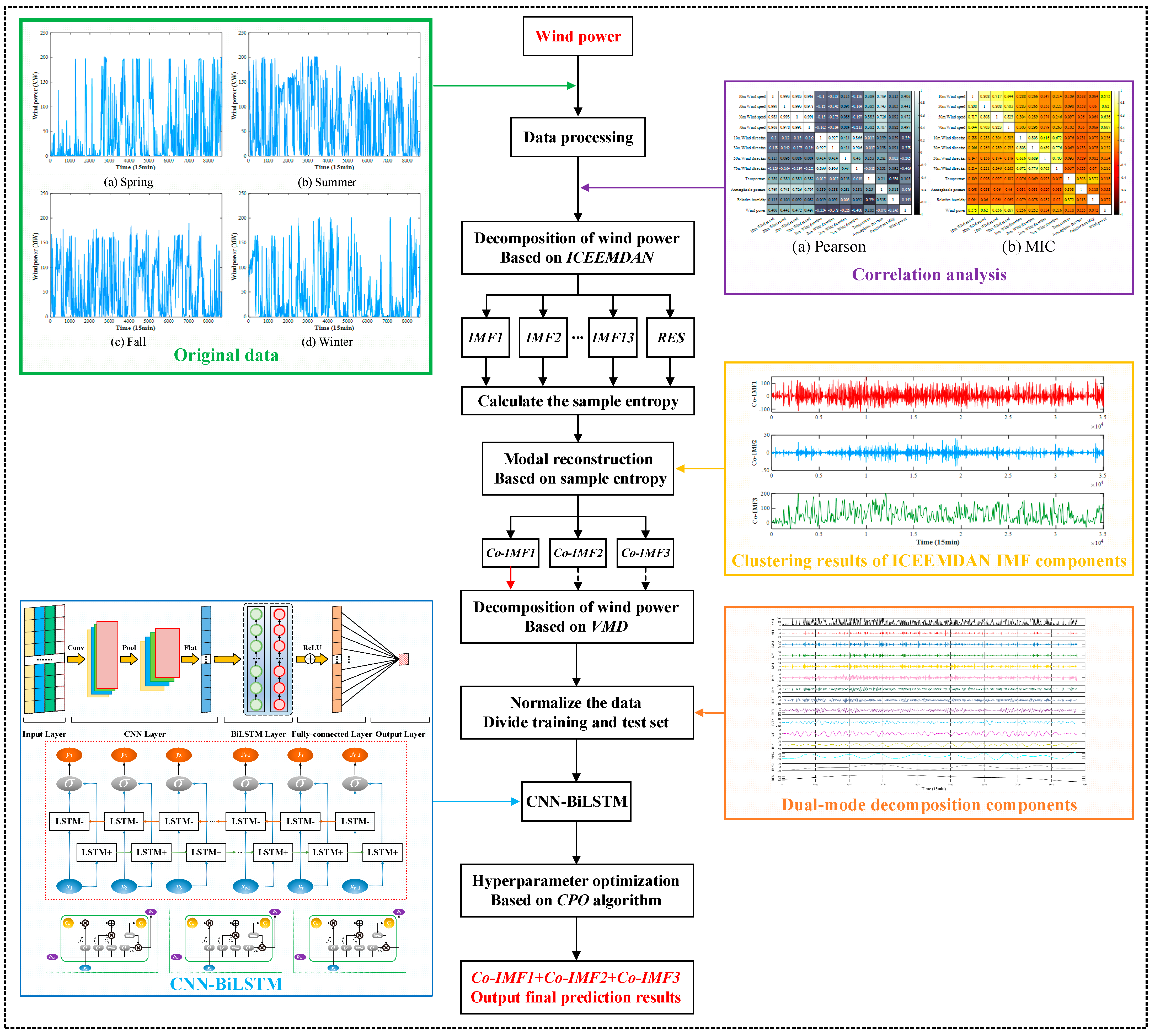
• An adaptive dual-stage signal preprocessing framework is proposed. Unlike conventional cascade decomposition methods that apply secondary decomposition to all components, the proposed framework uses sample entropy and K-Means clustering to assess the complexity of decomposed components. Secondary VMD is applied only to the high-frequency cluster with stronger volatility, which helps to reduce mode aliasing and avoid unnecessary decomposition of relatively stable components.
• A hybrid prediction model integrating CNN-BiLSTM with the Crested Porcupine Optimizer (CPO) is developed. CNN is used to extract local sequential features, and BiLSTM is used to capture bidirectional temporal dependencies. CPO is used to tune key hyperparameters of the prediction model, thereby reducing reliance on manual empirical parameter selection.
• The forecasting performance of the proposed method is evaluated using operational wind-farm data and benchmark models. The results indicate that the proposed framework yields lower prediction errors under the tested conditions and provides a data-driven reference for wind power forecasting, renewable-energy accommodation, and short-term power system dispatch.

2. Materials and Methods

2.1. Improved Complete Ensemble Empirical Mode Decomposition with Adaptive Noise

ICEEMDAN improves upon CEEMDAN by optimizing the customized addition of noise, significantly reducing residual noise and spurious components generated during signal decomposition. Applying the ICEEMDAN algorithm allows any signal to be decomposed into a superposition of multiple Intrinsic Mode Functions (IMFs) and a residual component, thereby enhancing the ability of the prediction model to identify characteristic information from collected wind farm data. The specific implementation process of the ICEEMDAN algorithm is as follows:

1.

As shown in Equation (1), a specific amount of white noise is added to the original signal set $x$ to obtain $x^{(i)}$.

$$x^{(i)}=x+{\beta }_0{E}_1\left(w^{(i)}\right)$$

(1)

where: $i$ is the number of noise additions ($i=1,2,\dots ,M$); $x^{(i)}$ is the signal set to be decomposed after noise addition; ${\beta }_0$ is the signal-to-noise ratio (SNR) for the initial decomposition of the signal; $w^{(i)}$ is the white noise, and $E_1(w^{(i)})$ is the first EMD component of the white noise.

2.

As shown in Equation (2), the first residual component $R_1$ is obtained.

$$R_1={\displaystyle \sum _{i=1}^{M}M\left(x^{(i)}\right)}$$

(2)

where: $M(\cdot )$ is the local mean envelope of the signal, used to determine the boundaries of the IMF.

3.

As shown in Equation (3), the initial modal component $IM{F}_1$ of ICEEMDAN is calculated.

$$IM{F}_1=x-R_1$$

(3)

4.

As shown in Equation (4), white noise is continuously added to obtain the k-th residual component $R_k$.

$$R_k={\displaystyle \sum _{i=1}^{M}M\left(R_{k-1}+{\beta }_{k-1}{E}_k\left(w^{(i)}\right)\right)} , k\ge 2$$

(4)

where: ${\beta }_{k-1}$ is the SNR for the k-th decomposition of the signal, and $E_k(w^{(i)})$ is the k-th EMD component of the white noise.

5.

As shown in Equation (5), the k-th modal component $IM{F}_k$ is calculated.

$$IM{F}_k=R_{k-1}-R_k, k\ge 2$$

(5)

6.

Step 5 is continuously executed until the signal can no longer be decomposed. When the residual part exhibits monotonicity and the threshold amplitude is greater than the residual part, the signal decomposition process is immediately stopped, yielding the final set of modal components.

2.2. Variational Mode Decomposition

VMD is an advanced signal decomposition technique possessing the capability to concurrently process both recursive and non-recursive signals. It reformulates the complex signal decomposition task into a variational problem. The specific steps of VMD are outlined as follows:

1.

As depicted in Equation (6), VMD defines its objective function as the minimization of the sum of the estimated bandwidths of the decomposed modes. For each modal component, its analytic signal $u_k(t)$ is computed via the Hilbert transform to obtain the unilateral spectrum. Subsequently, by incorporating the Gaussian smoothness of this signal, its center frequency is estimated and utilized as an exponential multiplicative factor to shift the signal to its respective baseband, thereby formulating a constrained variational problem.

$$\begin{gathered} \underset{\left\{u_k\right\},\left\{{\omega }_k\right\}}{\min }\left\{{\displaystyle \sum _k{‖{\partial }_t\left[\left(\delta (t)+\frac{j}{\pi t}\right)\ast u_k(t)\right]e^{-j{\omega }_{k}t}‖}_2^2}\right\} \\ s.t. {\displaystyle \sum _k{u}_k=f(t)} \end{gathered}$$

(6)

where: $f(t)$ is the original input signal; $u_k(t)$ and ${\omega }_k(t)$ are the k-th modal component and its center frequency, respectively; $\delta (t)$ is the Dirac delta function; and $\ast$ is the convolution operator.

2.

As shown in Equation (7), the constrained variational problem is transformed into an unconstrained one by introducing a Lagrange multiplier $\lambda (t)$ and a penalty factor $\alpha$. This transformation, particularly in the presence of Gaussian noise interference, serves to simplify the solution process and attenuate the impact of noise.

$$\begin{array}{r}L\left(\left\{u_k\right\},\left\{{\omega }_k\right\},\lambda \right)=\alpha {\displaystyle \sum _{k=1}^K{‖{\partial }_t\left[\left(\delta (t)+\frac{j}{\pi t}\right)\ast u_k(t)\right]e^{-j{\omega }_{k}t}‖}_2^2}\\ +{‖f(t)-{\displaystyle \sum _k{u}_k(t)}‖}_2^2+〈\lambda (t),f(t)-{\displaystyle \sum _k{u}_k(t)}〉\end{array}$$

(7)

3.

As shown in Equation (8), the Alternating Direction Method of Multipliers (ADMM) is applied to solve for the minimum of the augmented Lagrange expression in Equation (7). The optimal solution yields the modal components $IMF\left\{u_k\right\}$ and the center frequencies $\left\{{\omega }_k\right\}$. The iteration terminates when the convergence tolerance constraint $\epsilon$ = 1 × 10⁻⁶ is satisfied between consecutive updates.

$${\displaystyle \sum _k\frac{{‖{\widehat{u}}_k^{n+1}-{\widehat{u}}_k^n‖}_2^2}{{‖{\widehat{u}}_k^n‖}_2^2}}<\epsilon$$

(8)

4.

As shown in Equation (9), after convergence through alternating updates, the frequency bands are partitioned based on the frequency-domain characteristics of the modes, ultimately achieving the adaptive modal decomposition of the signal.

$${\widehat{u}}_k^{n+1}(\omega )={\displaystyle \frac{\widehat{x}(\omega )-{\displaystyle {\sum }_{i<k}{\widehat{u}}_i^n(\omega )+0.5\ast \widehat{\lambda }(\omega )}}{1+2\alpha {\left(\omega -{\omega }_k\right)}^2}}$$

(9)

2.3. Convolutional Neural Network

CNN is a feedforward neural network that incorporates convolutional operations and possesses a deep structure, exhibiting strong nonlinear feature extraction capabilities. It is frequently employed to address issues such as the loss of temporal information and training overfitting. CNNs are primarily composed of convolutional layers, pooling layers, and fully connected layers. Within the convolutional layers, multiple convolutional kernels are contained, and each element constituting a convolutional kernel corresponds to a weight coefficient and a bias coefficient to perform deep feature extraction.

2.4. Bi-Directional Long-Short Term Memory

To address issues such as gradient explosion inherent in traditional Recurrent Neural Networks, the LSTM network was proposed to handle long-term sequence tasks. However, during the process of sequential training, LSTM can only process feature information propagated through the forward channel, failing to maximally extract the internal correlations within wind power output sequences. Therefore, compared to the unidirectional LSTM network, employing a BiLSTM network allows for better learning of key features from bidirectional time-series data, enabling the capture of more sequence information [31]. Furthermore, BiLSTM can simultaneously extract and store bidirectional neuronal information, thereby more effectively fitting the ultra-short-term temporal dependencies in wind power. The operational principle of BiLSTM is illustrated in Figure 2.

The sequential data processing in BiLSTM comprises three gating mechanisms: the forget gate $f_t$, the input gate $i_t$, and the output gate $o_t$, as shown in Equations (10)–(15).

$$f_t=\sigma \left(W_f^{+}{x}_t+B_f^{+}+W_f^{-}{h}_{t-1}+B_f^{-}\right)$$

(10)

$$i_t=\sigma \left(W_i^{+}{x}_t+B_i^{+}+W_i^{-}{h}_{t-1}+B_i^{-}\right)$$

(11)

$$o_t=\sigma \left(W_o^{+}{x}_t+B_o^{+}+W_o^{-}{h}_{t-1}+B_o^{-}\right)$$

(12)

$${\tilde{C}}_t=\tanh \left(W_c^{+}{x}_t+B_c^{+}+W_c^{-}{h}_{t-1}+B_c^{-}\right)$$

(13)

$$c_t=f_t\odot c_{t-1}+i_t\odot {\tilde{C}}_t$$

(14)

$$h_t=o_t\odot \tanh \left(c_t\right)$$

(15)

where: $W$ represents the corresponding weight parameters, $B$ represents the corresponding bias parameters, (+) and (−) indicate the forward and backward directions, respectively; $c_t$ represents the current cell state, ${\tilde{C}}_t$ represents the candidate cell state, and $h_t$ represents the current hidden state; $\sigma$ represents the sigmoid activation function, which maps variables to the interval [0, 1].

At each time step t, the BiLSTM concatenates the forward and backward hidden states to obtain the final hidden state representation $h_t^{final}=[h_t^{+},h_t^{-}]$ for that time step. This representation is used for the final prediction output.

2.5. Crested Porcupine Optimizer (CPO)

CPO is an optimization algorithm proposed by Reference [32], inspired by the diverse defense behaviors of the Crested Porcupine (CP) in nature. Compared to conventional optimizers such as PSO or GWO, the CPO algorithm enforces a mathematical balance between exploration and exploitation through its Cyclic Population Reduction (CPR) mechanism and four distinct defense strategies [33]. This structural property mitigates premature convergence when navigating the high-dimensional hyperparameter spaces of deep neural networks. Recent offshore-wind studies have used meta-heuristic optimizers to tune fractional-order PID control and optimal control strategies, indicating that such optimizers have been applied in renewable-energy control problems [34,35]. CPO employs four distinct mechanisms: visual, auditory, olfactory, and physical attack. The first and second defense strategies reflect exploration behavior, while the third and fourth defense strategies reflect exploitation behavior.

As shown in Equation (16), CPO algorithm adopts a novel strategy based on the Cyclic Population Reduction (CPR) technique to accelerate convergence speed.

$$N=N_{\min }+\left(N^{\prime }-N_{\min }\right)\times \left(1-\left(\left(t\%{\displaystyle \frac{T_{\max }}{T}}\right)/{\displaystyle \frac{T_{\max }}{T}}\right)\right)$$

(16)

where: T is a variable that determines the number of cycles; t is the current iteration number; $T_{\max }$ is the maximum number of iterations; % represents the modulo or remainder operator; and $N_{\min }$ is the minimum allowable population size.

2.5.1. Exploration Phase

• First defensive strategy

As shown in Equation (17), when the CP becomes aware of a predator’s presence, it adopts the first defense strategy. The predator has two choices: (1) To approach, which encourages exploration of the region between the predator and the CP to accelerate convergence speed; (2) To move away, which encourages exploration of unknown regions to perform global optimization and avoid entrapment in local optima.

$$\overrightarrow{x_i^{t+1}}=\overrightarrow{x_i^t}+{\tau }_1\times \left|2\times {\tau }_2\times \overrightarrow{x_{CP}^t}-\overrightarrow{y_i^t}\right|$$

(17)

where: $\overrightarrow{x_{CP}^t}$ is the optimal solution of the evaluation function; $\overrightarrow{x_i^t}$ is the position of the i-th CP individual at iteration t; $\overrightarrow{y_i^t}$ is a vector generated between the current CP and a randomly selected CP from the population, representing the position of the predator at iteration t; ${\tau }_1$ is a random value based on a normal distribution; and ${\tau }_2$ is a random value in the interval [0, 1].

2.

Second defensive strategy

As shown in Equation (18), in this strategy, the CP creates noise and threatens the predator. When the predator approaches, the CP intensifies its vocalizations.

$$\overrightarrow{x_i^{t+1}}=\left(1-\overrightarrow{U_1}\right)\times \overrightarrow{x_i^t}+\overrightarrow{U_1}\times \left(\overrightarrow{y}+{\tau }_3\times \left(\overrightarrow{x_{r_1}^t}-\overrightarrow{x_{r_2}^t}\right)\right)$$

(18)

where: $r_1$ and $r_2$ are random numbers within the interval [1, N]; ${\tau }_3$ is a random value within the interval [0, 1]; and $\overrightarrow{U_1}$ is a binary vector containing 0 and 1, to cover all possible chosen actions.

2.5.2. Exploitation Phase

• Third defensive strategy

As shown in Equation (19), in this strategy, the CP secretes a foul odor and disseminates it in the surrounding area to deter predators from approaching.

$$\overrightarrow{x_i^{t+1}}=\left(1-\overrightarrow{U_1}\right)\times \overrightarrow{x_i^t}+\overrightarrow{U_1}\times \left(\overrightarrow{x_{r_1}^t}+S_i^t\times \left(\overrightarrow{x_{r_2}^t}-\overrightarrow{x_{r_3}^t}\right)-{\tau }_3\times \overrightarrow{\delta }\times {\gamma }_t\times S_i^t\right)$$

(19)

where: $r_3$ is a random number within the interval [1, N]; $\overrightarrow{\delta }$ is a parameter controlling the search direction; ${\gamma }_t$ is a predefined defense factor; and $S_i^t$ is a predefined odor diffusion factor.

2.

Fourth defensive strategy

As shown in Equation (20), in this strategy, the CP initiates a physical attack, during which two objects undergo an inelastic collision.

$$\overrightarrow{x_i^{t+1}}=\overrightarrow{x_{CP}^t}+\left(a\left(1-{\tau }_4\right)+{\tau }_4\right)\times \left(\delta \times \overrightarrow{x_{CP}^t}-\overrightarrow{x_i^t}\right)-{\tau }_5\times \delta \times {\gamma }_t\times \overrightarrow{F_i^t}$$

(20)

where: $a$ is a predefined convergence speed factor; ${\tau }_4$ and ${\tau }_5$ are random values in the interval [0, 1]; and $\overrightarrow{F_i^t}$ is the average force of the CP affecting the i-th predator, provided by the laws of inelastic collision.

As shown in the pseudo-code Algorithm 1 [32], the procedure for optimizing and tuning the CNN-BiLSTM model using the CPO algorithm is presented.

Algorithm 1 Pseudo-code of CPO: Hyperparameter optimization of CNN-BiLSTM

Input: hyperparameter optimization range for the CNN-BiLSTM Set parameters: convergence speed factor $\alpha$; trade-off coefficient $T_f$; current iteration number T; Initialize the solutions’ positions randomly; While $t\le T_{max}$     Evaluate fitness values for the candidate solutions;     Determine the best ($\overrightarrow{x_{CP}^t}$) solution so far;     Update the defense factor $y_t$     Update the population size N

For $i=1 :N$ Update the m, S, F, $\overrightarrow{\delta }$ Generate two random numbers ${\tau }_8$ and ${\tau }_9$ If ${\tau }_8<{\tau }_9$//Turn to Exploration phase             Generate two random numbers ${\tau }_6$ and ${\tau }_7$

If ${\tau }_6<{\tau }_7$, Apply Equation (17)//Turn to First defense strategy

Else Apply Equation (18)//Turn to Second defense strategy

Else//Turn to Exploration phase             Generate a random number ${\tau }_{10}$      If ${\tau }_{10}<T_f$, Apply Equation (19)//Turn to Third defense strategy

Else Apply Equation (20)//Turn to Fourth defense strategy          End If          If $f\left({\overrightarrow{x}}_i^{t+1}\right)>f\left({\overrightarrow{x}}_i^t\right)$             ${\overrightarrow{x}}_i^{t+1}={\overrightarrow{x}}_i^t$          End If          $t=t+1$ End For End While Return the best solution ($\overrightarrow{x_{CP}^t}$)

Output: optimal hyperparameter combination of CNN-BiLSTM

3. Results

3.1. Data Description and Experimental Environment

The experimental data in this paper were sourced from the China Xinjiang Guohua Jingxia North Wind Farm and the local meteorological bureau. The experimental dataset, spanning from 1 January 2019 to 31 December 2019, encompasses wind power data and meteorological data. The data were sampled at 15 min intervals, with wind power measured in MW, yielding a total of 35,040 data points. The time series of original wind power data for each season is shown in Figure 3. During the experimental process, the dataset was partitioned into training and testing sets at an 8:2 ratio. The wind farm comprises 133 wind turbines, each with 1.5 MW capacity, and total installed capacity of 199.5 MW.

The computational platform was primarily configured with a Windows 11 operating system, a 12th Gen Intel^® Core™ i7-12700H CPU, an RTX 3070Ti GPU, and 16 GB of RAM. The development of the prediction model proposed in this paper was implemented using MATLAB 2024b programming.

Table 1. Model and algorithm parameter settings.

Method	Parameter	Value
CNN-BiLSTM	Sequence-input Layer	/
	Sequence-folding Layer	/
	Convolution Layer	filters = 16, size = [3, 1]
	Batch-normalization Layer	/
	Activation function	ReLU
	Max-pooling Layer	size = [2, 1]
	Sequence-unfolding Layer	/
	Flatten Layer	/
	Dropout ratio	0.1
	Fully connected Layer	1
	Regression Layer	/
	Optimizer	Adam
ICEEMDAN-VMD	Noise Standard Deviation	0.2
	Number of Realizations	50
	Max Iteration	1000
	Signal-to-Noise Ratio Flag	1
	Number of Clustering	3
	IMFs Number	5
	Penalty Factor	2500

details the architecture of the employed neural networks and their specific algorithmic parameters. Other hyperparameters, such as the learning rate, regularization parameters, and the number of hidden units, were determined via a hyperparameter optimization algorithm, thereby avoiding the weak interpretability and unscientific nature of manual parameter tuning.

To prevent temporal data leakage, all data normalization scalers and signal decomposition baseline parameters were fitted solely on the training set and subsequently applied to the testing set via a sliding window protocol. The model utilizes a rolling 1-step ahead forecasting horizon, which corresponds to a 15-min ahead prediction based on the data sampling interval. During the model training phase, the batch size is set to 64, the maximum number of training epochs is 100, and the Adam optimizer is utilized. A linear activation function is applied in the final fully connected layer preceding the continuous regression output. The termination criterion for the CPO algorithm is set to reach the predefined maximum number of iterations.

3.2. Data Preprocessing

In this section, Pearson correlation analysis is employed to examine the linear relationships between wind power and wind speed, wind direction, temperature, air pressure, and humidity. However, as nonlinear, deep internal connections also exist between wind power and these features, the MIC algorithm is subsequently utilized for nonlinear correlation analysis. The Pearson coefficient is presented in Equation (21), and the MIC is presented in Equations (22) and (23).

$$P(x_i,y_i)={\displaystyle \frac{{\displaystyle \sum _{i=1}^N(x_i-\overline{x})(y_i-\overline{y})}}{\sqrt{{\displaystyle \sum _{i=1}^N{(x_i-\overline{x})}^2{(y_i-\overline{y})}^2}}}}$$

(21)

$$I(x_i,y_i)={\displaystyle \int p(x_i,y_i){\log }_2}{\displaystyle \frac{p(x_i,y_i)}{p(x_i)p(y_i)}}dxdy$$

(22)

$$f_{mic}(x_i,y_i)=\underset{ab<B}{\max }{\displaystyle \frac{I(x_i,y_i)}{{\log }_2\min (a,b)}}$$

(23)

where: $x_i$ and $y_i$ are the variables under analysis; $p(x_i,y_i)$ is the joint probability of the variables; $f_{mic}$ is the maximal information coefficient; a and b are the dimensions (number of bins) of the grid partition; B is the sample size raised to the power of 0.6.

The specific results of the correlation analysis are presented in Figure 4 and

Table 2. Correlation analysis.

Feature	Correlation Coefficient
	Pearson	Value
10 m Wind speed	0.406	0.575
30 m Wind speed	0.441	0.620
50 m Wind speed	0.472	0.656
70 m Wind speed	0.497	0.667
10 m Wind direction	−0.354	0.256
30 m Wind direction	−0.378	0.252
50 m Wind direction	−0.205	0.134
70 m Wind direction	−0.406	0.216
Temperature	0.105	0.118
Atmospheric pressure	−0.076	0.055
Relative humidity	−0.145	0.072

. Using $\left|P\right|>0.3$ and $f_{mic}>0.2$ as comprehensive screening thresholds, features with weaker correlation coefficients are eliminated, and the remaining parameters are selected as input features.

Subsequently, the ICEEMDAN-VMD algorithm is employed to decompose the wind power sequence after feature selection, thereby attenuating residual noise in the data and providing more regular input features for the CNN-BiLSTM prediction model.

First, the original wind power sequence is subjected to an initial decomposition using the Improved Complete Ensemble Empirical Mode Decomposition with Adaptive Noise (ICEEMDAN) algorithm, as specified in Equations (1)–(5). This process yields a set of Intrinsic Mode Function (IMF) components and a residual (RES), which are illustrated in Figure 5. Subsequently, to group these components based on their physical characteristics, the sample entropy of each IMF is calculated. The K-Means clustering algorithm (with K = 3) is then employed to categorize the IMFs into three distinct clusters: a high-frequency component (Co-IMF1), a medium-frequency component (Co-IMF2), and a low-frequency component (Co-IMF3). The results of this clustering are shown in Figure 6: Co-IMF1 encapsulates the most volatile and random fluctuations, Co-IMF2 represents relatively stable periodicities, and Co-IMF3 captures the primary trend of the wind power signal.

Applying VMD to all decomposed modes increases computational burden and risks altering the stable low-frequency trend components (Co-IMF3). The high-frequency cluster (Co-IMF1), however, contains a mixture of stochastic meteorological noise and abrupt signal variations. Therefore, a secondary decomposition using Variational Mode Decomposition (VMD) is performed exclusively on Co-IMF1 in accordance with Equations (6)–(9). This targets localized high-frequency complexity without degrading the primary power generation trends. This step refines the high-frequency signal into a set of sub-modes (Co-IMF1(1), Co-IMF1(2), Co-IMF1(3)), as depicted in Figure 7. Finally, the sub-modes derived from the VMD of Co-IMF1 are combined with the original Co-IMF2 and Co-IMF3 components. This consolidated set of multi-scale features constitutes the final input for the subsequent prediction model.

As observed from the decomposition results in Figure 6 and Figure 7, the proposed ICEEMDAN-VMD dual-decomposition strategy effectively deconstructs the original non-stationary wind power sequence into a series of modal components, each exhibiting distinct frequency scales and fluctuation characteristics. The secondary VMD applied to the high-frequency component, Co-IMF1, markedly improves the stationarity and regularity of its sub-modes while successfully isolating high-frequency noise. Concurrently, the medium- and low-frequency components clearly reveal the primary trends and periodic features of the wind power signal at different time scales. By alleviating the non-stationarity and non-linearity of the original signal and attenuating noise interference, this decomposition strategy empowers the model to more effectively capture the complex dynamics of wind power, thereby enhancing prediction accuracy on ultra-short-term time scales.

3.3. Evaluation Criteria

To objectively evaluate the model performance of the proposed prediction method, Root Mean Square Error (RMSE) is used as the metric for the optimization algorithm to select the optimal hyperparameter combination. RMSE, Mean Absolute Error (MAE), Mean Absolute Percentage Error (MAPE), and R-squared (R²) are employed to quantify the model’s prediction performance, serving as evaluation metrics for the accuracy of the prediction model, as shown in Equations (24)–(27).

$$RMSE=\sqrt{{\displaystyle \frac{1}{N}}{\displaystyle \sum _{i=1}^N{\left({\tilde{y}}_i-y_i\right)}^2}}$$

(24)

$$MAE={\displaystyle \frac{1}{N}}{\displaystyle \sum _{i=1}^N\left|{\tilde{y}}_i-y_i\right|}$$

(25)

$$MAPE={\displaystyle \frac{100\%}{N}}{\displaystyle \sum _{i=1}^N\left|\frac{{\tilde{y}}_i-y_i}{y_i}\right|}$$

(26)

$$R^2=1-\sqrt{{\displaystyle \sum _{i=1}^N{\left({\tilde{y}}_i-y_i\right)}^2}}/\sqrt{{\displaystyle \sum _{i=1}^N{\left(y_i-{\overline{y}}_i\right)}^2}}$$

(27)

3.4. Case Study Analysis

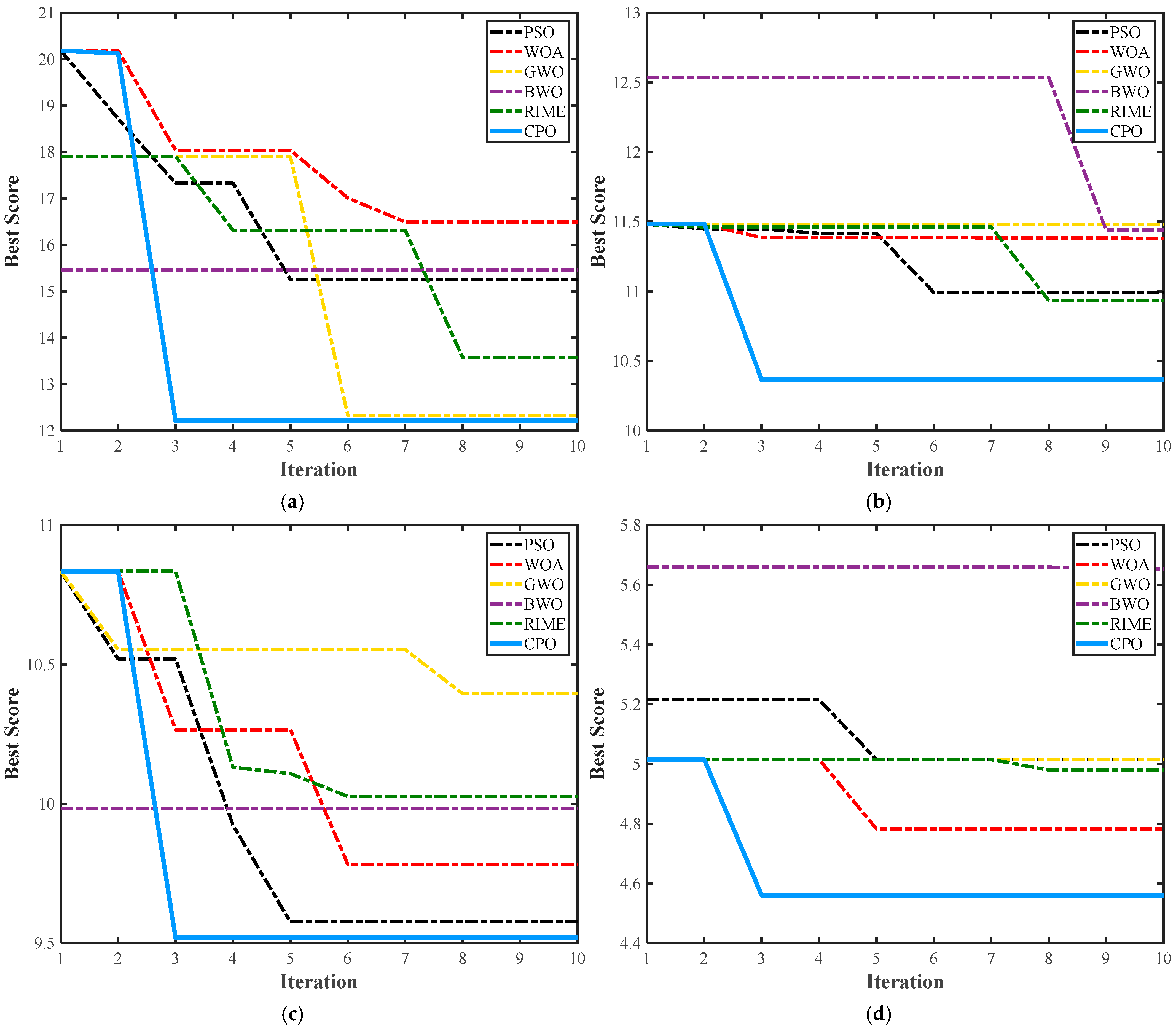
3.4.1. Analysis of Optimization Algorithm

This section aims to evaluate the performance of different heuristic optimization algorithms in the hyperparameter optimization task for the CNN-BiLSTM model and to validate the superiority of the CPO algorithm adopted in this paper. For comparison, five other algorithms, namely PSO [36], WOA [37], GWO [38], BWO [39] and RIME [40], were selected. RMSE was utilized as the metric to assess the optimization effectiveness of each algorithm across different seasons.

Table 3. Optimization algorithm performance metrics (RMSE ↓).

Algorithm	Spring	Summer	Fall	Winter
PSO	15.251	10.991	9.576	5.015
WOA	16.493	11.379	9.783	4.783
GWO	12.329	11.481	10.396	5.015
BWO	15.456	11.441	9.982	5.652
RIME	13.576	10.936	10.026	4.980
CPO	12.215	10.365	9.520	4.560

↓ indicates decrease.

lists the lowest RMSE values achieved by the six optimization algorithms after optimizing the CNN-BiLSTM model on the datasets for the four seasons, and Figure 8 illustrates their corresponding fitness iteration curves. The CPO algorithm achieved the minimum RMSE on the datasets for all seasons compared to the other evaluated algorithms. Furthermore, the convergence curves indicate that the CPO algorithm converges to the lowest fitness value and exhibits a faster convergence rate in these test cases. In the spring and autumn datasets, the algorithm reaches lower fitness values in earlier iterations. These results indicate that, when searching the hyperparameter space of the CNN-BiLSTM model, the CPO algorithm maintains a balance between global exploration and local exploitation. It avoids premature convergence to local optima, thereby identifying a hyperparameter configuration that corresponds to lower prediction errors.

3.4.2. Analysis of Forecasting Result

This section aims to evaluate the overall performance of the proposed method in the ultra-short-term wind power forecasting task. To this end, datasets from two representative seasons, summer and winter, were selected for simulation experiments. Through ablation studies, the proposed method was compared with four benchmark or simplified models: CNN-BiLSTM, VMD-CNN-BiLSTM, CEEMDAN-CNN-BiLSTM, and CEEMDAN-VMD-CNN-BiLSTM, to validate the effectiveness of each component and the superiority of the overall model.

The comparison of various evaluation metrics for wind power forecasting in the summer and winter seasons is presented in

Table 4. Comparison of predictive evaluation criteria (summer).

Model	RMSE (↓)	MAE (↓)	MAPE (↓)	R2 (↑)
CNN-BiLSTM	11.8376	8.5917	16.1973%	91.9533%
VMD-CNN-BiLSTM	9.1406	6.7407	11.7021%	95.3463%
CEEMDAN-CNN-BiLSTM	8.5515	6.3423	7.2675%	95.8008%
CEEMDAN-VMD-CNN-BiLSTM	8.3916	6.2549	10.0738%	95.9564%
CPO-ICEEMDAN-VMD-CNN-BiLSTM	7.5262	5.5792	9.0575%	96.7473%

↑ and ↓ indicate increase and decrease.

and

Table 5. Comparison of predictive evaluation criteria (winter).

Model	RMSE (↓)	MAE (↓)	MAPE (↓)	R2 (↑)
CNN-BiLSTM	21.0519	15.3371	16.6057%	83.7359%
VMD-CNN-BiLSTM	14.3166	11.4413	9.2967%	92.5754%
CEEMDAN-CNN-BiLSTM	16.0613	11.2530	10.6153%	90.5331%
CEEMDAN-VMD-CNN-BiLSTM	10.5157	7.9958	7.9199%	95.9419%
CPO-ICEEMDAN-VMD-CNN-BiLSTM	9.2353	6.9161	7.3790%	96.8699%

↑ and ↓ indicate increase and decrease.

; the time-series prediction comparison curves are shown in Figure 9 and Figure 10; the absolute error violin plots are depicted in Figure 11; and the prediction error distributions (relative error) are illustrated in Figure 12.

1.

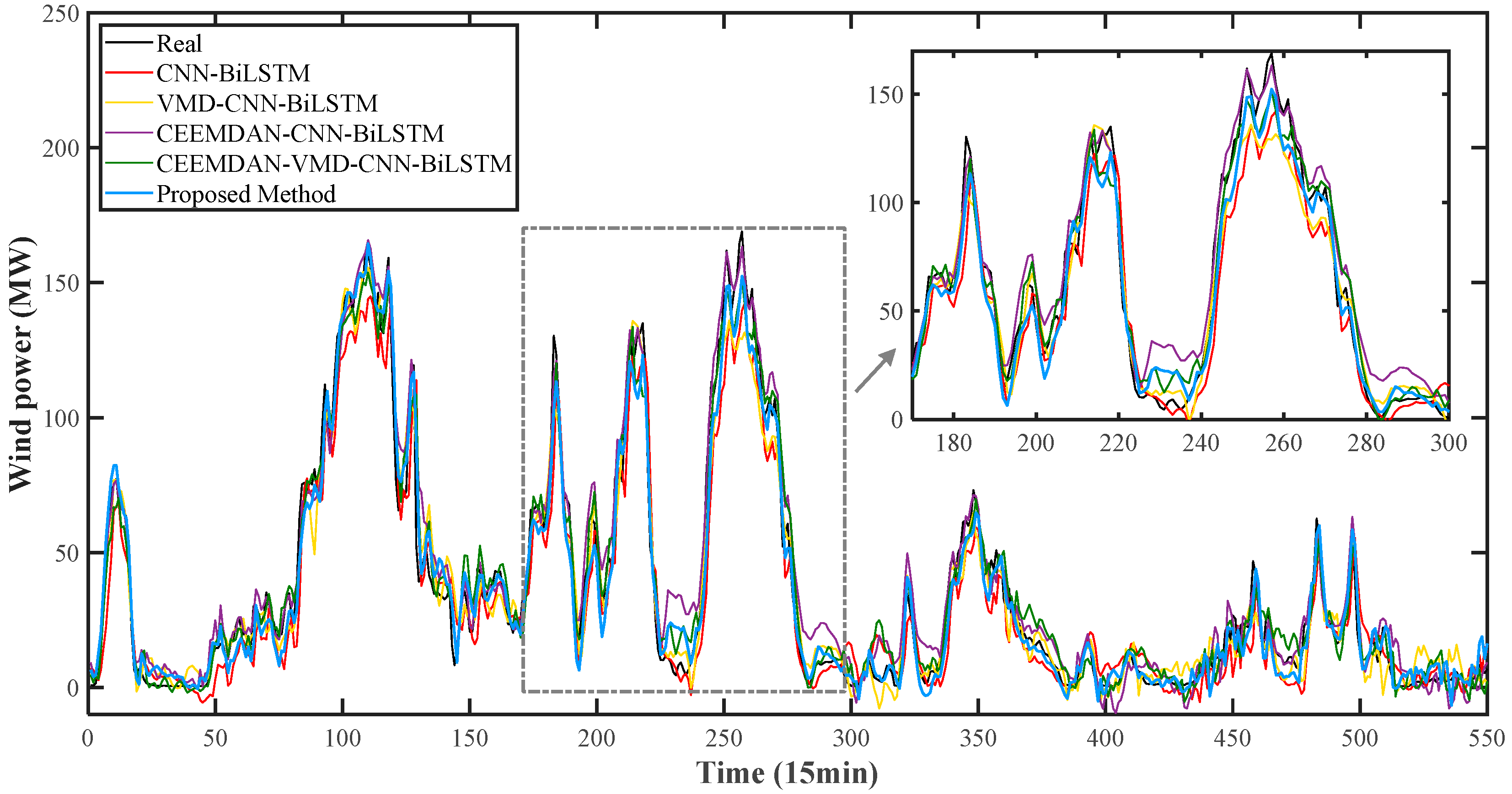
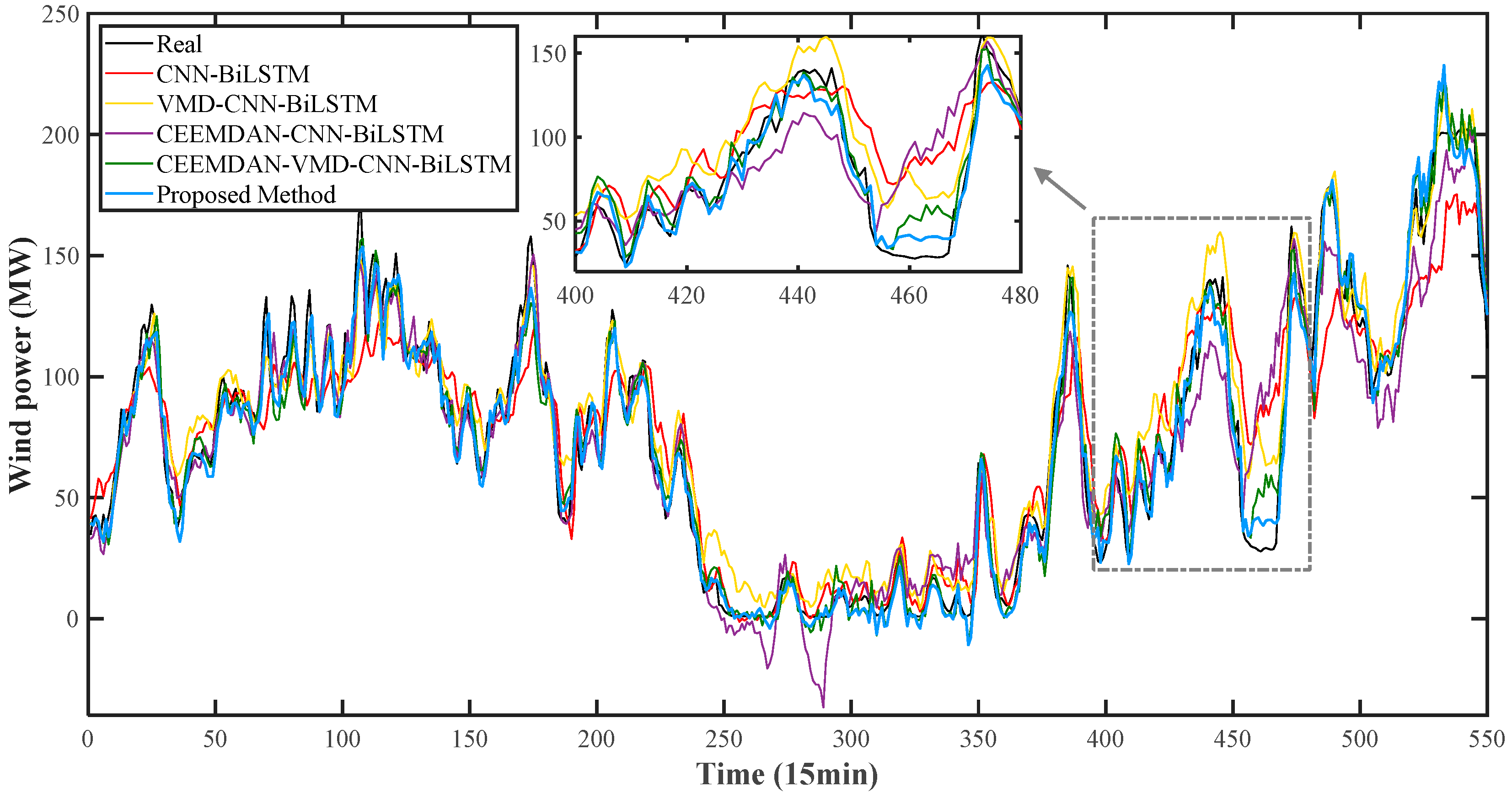
Regarding quantitative metrics, in both seasons, the evaluation metrics of the proposed method were lower in error and higher in R² compared to the other four models. Compared to the basic CNN-BiLSTM model, the proposed method reduced RMSE, MAE, and MAPE by approximately 36.4%, 35.1%, and 44.1%, respectively, and increased R² by approximately 5.2% in summer. In winter, RMSE, MAE, and MAPE decreased by approximately 56.1%, 54.9%, and 55.6%, respectively, and R² increased by approximately 15.7%. The ablation study results indicate that introducing VMD or CEEMDAN decomposition individually, or adopting the CEEMDAN-VMD dual decomposition strategy, all reduce prediction errors to varying degrees, with the CEEMDAN-VMD dual decomposition strategy yielding lower errors than single decomposition methods. The combination of the CPO optimization algorithm and the ICEEMDAN-VMD decomposition method corresponds to the lowest prediction errors among the tested models.

2.

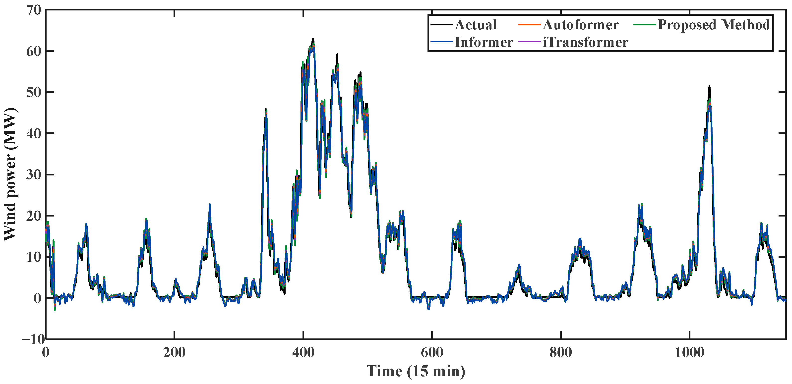
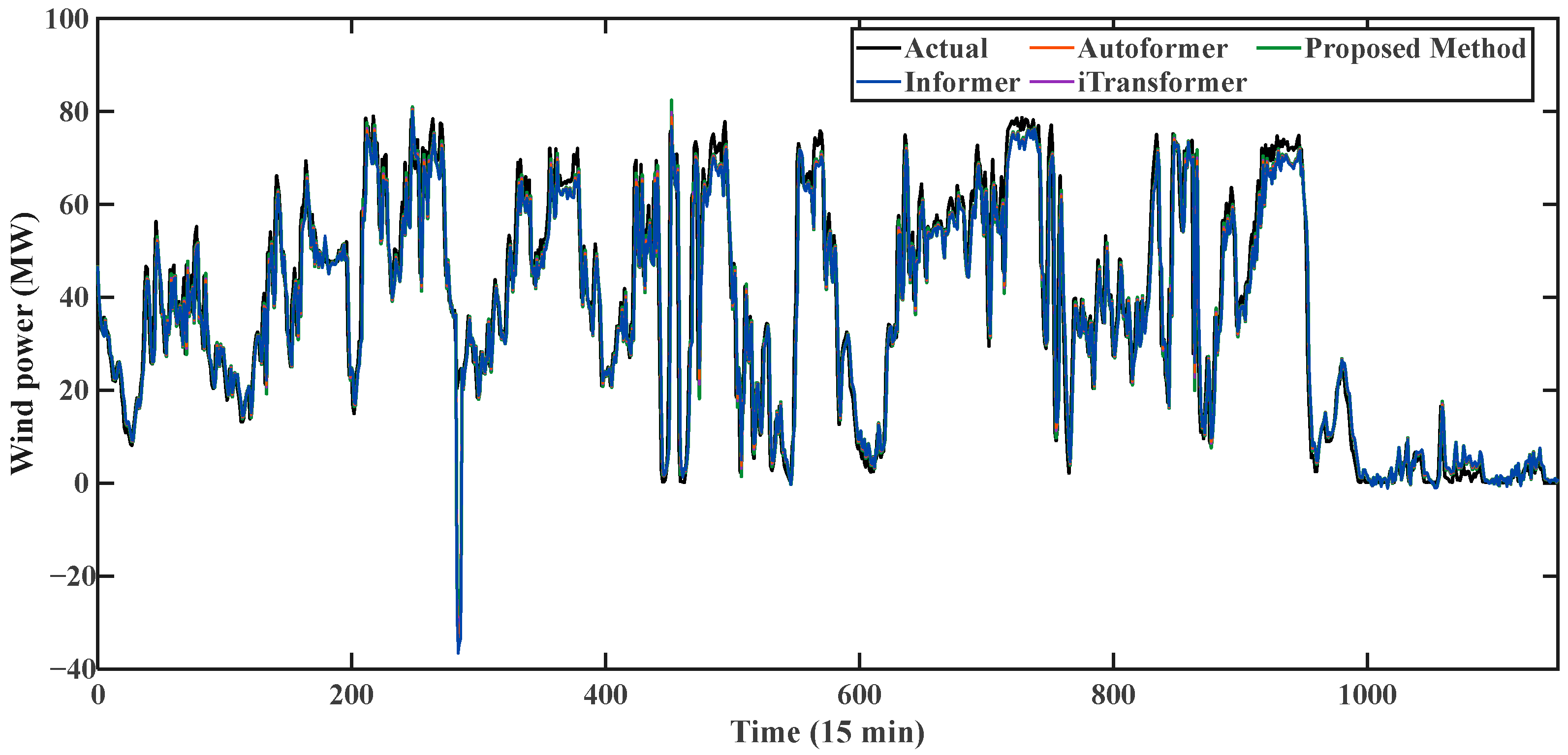
Regarding prediction curve fitting, the prediction curve of the proposed method (shown as the blue curve in Figure 9 and Figure 10) tracks the actual wind power fluctuations in both summer and winter seasons, including during periods of intense power fluctuation, which corresponds to the higher R² values reported.

3.

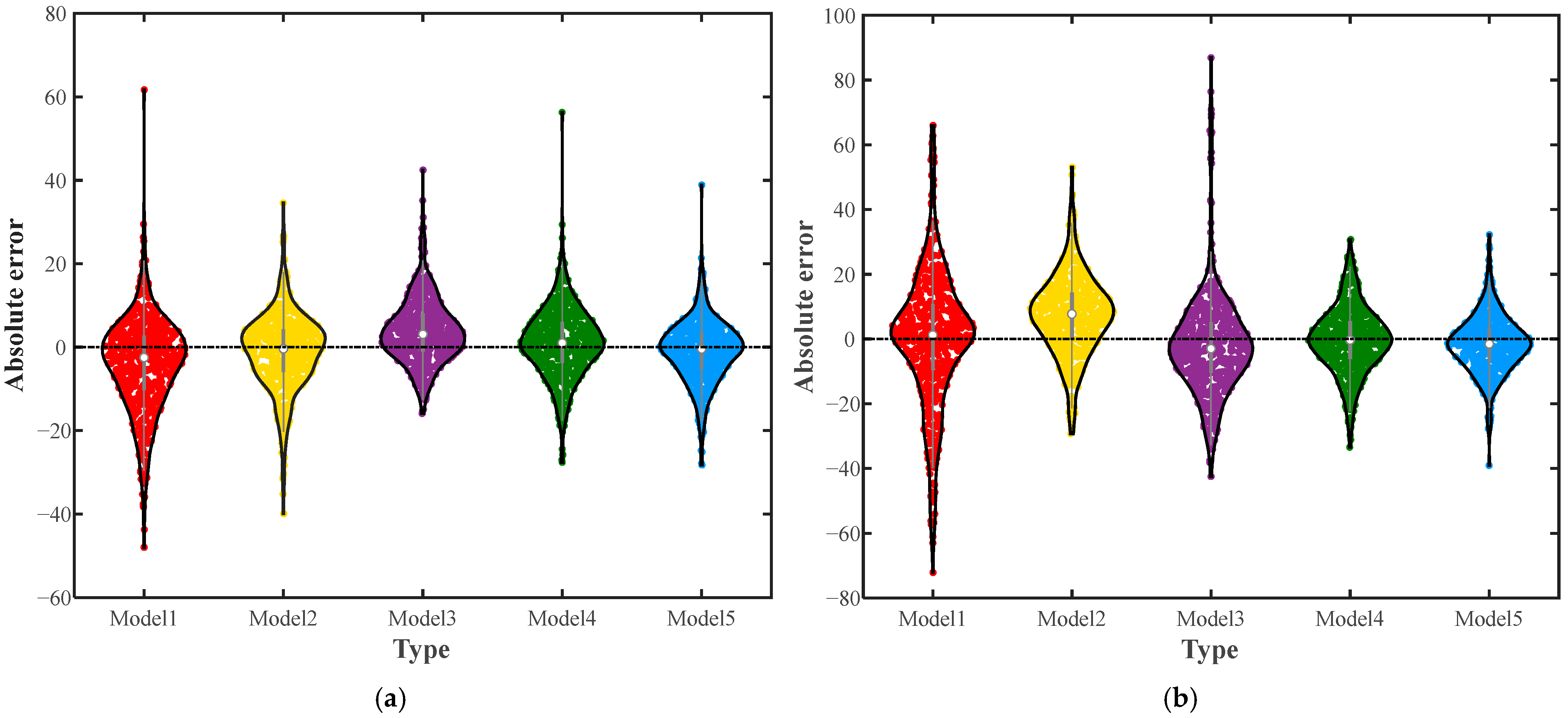
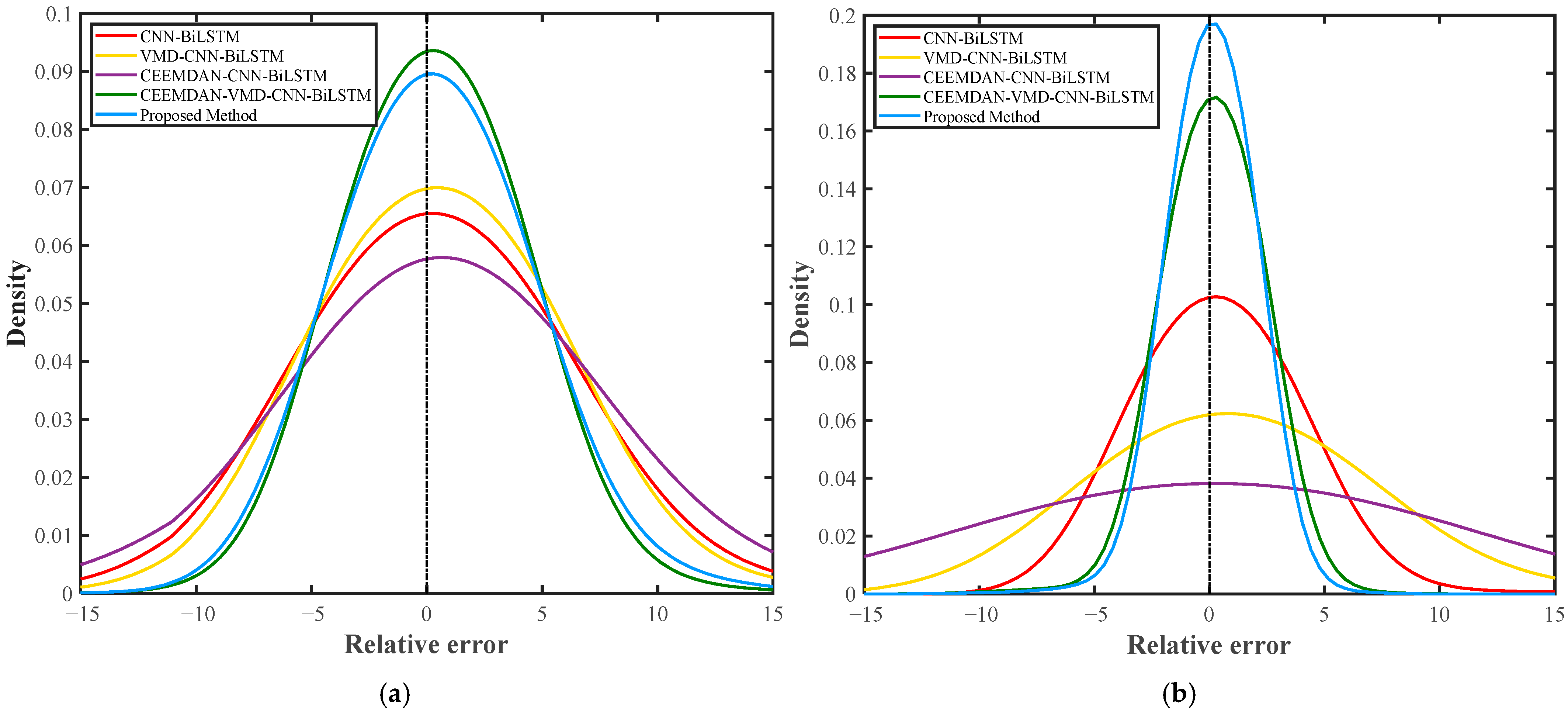
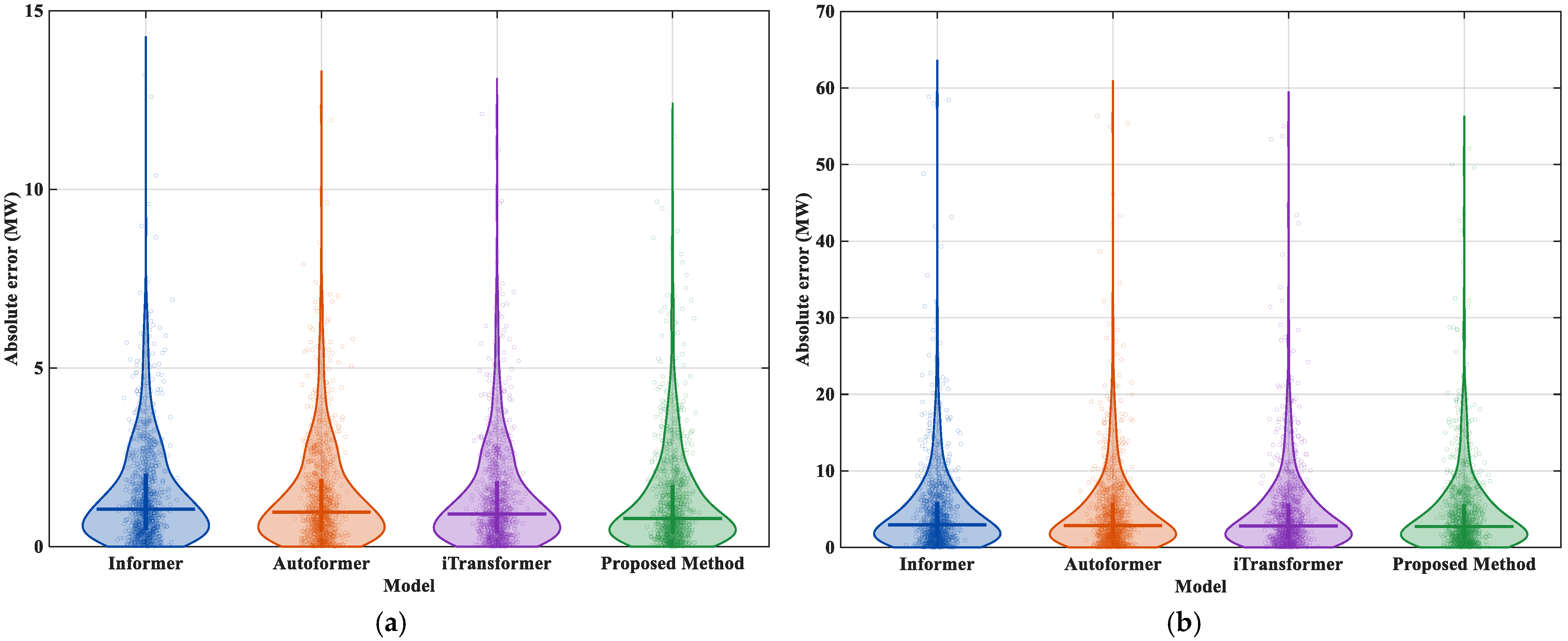
Concerning error distribution characteristics, the absolute error violin plots in Figure 11 show that the absolute error distribution of the proposed method is more concentrated in both seasons, with its median error and interquartile range being smaller than those of the comparative models. Furthermore, observing the probability density distribution of relative prediction errors (after Gaussian smoothing) shown in Figure 12: In the winter dataset, the error distribution curve of the proposed method exhibits the highest peak and the narrowest tails, indicating smaller prediction bias and a lower frequency of large errors compared to other models. In the summer dataset, although the peak of the Proposed Method’s error distribution curve is slightly lower than that of the CEEMDAN-VMD-CNN-BiLSTM model, its overall error distribution maintains a smaller interquartile range and overall bias relative to the basic models.

3.5. Advanced Baseline Comparison on External Datasets

To evaluate model generalization and compare with other baseline models, additional experiments were conducted on an external wind-power dataset sourced from [41]. Case 1 uses the Winter-2019 segment and Case 2 uses the Summer-2019 segment from Wind farm site 1, with a nominal capacity of 99 MW. These two seasonal cases provide additional scenarios to examine the proposed method.

The benchmark models include Informer [42], Autoformer [43], and iTransformer [44]. These models represent recent Transformer-based forecasting architectures.

Table 6. Advanced baseline comparison on two external wind-power cases.

Case	Model	RMSE (↓)	MAE (↓)	R2 (↑)
Case 1	Informer	2.0921	1.4825	0.9786
	Autoformer	2.0140	1.4067	0.9801
	iTransformer	1.9749	1.3654	0.9809
	Proposed Method	1.9194	1.2858	0.9820
Case 2	Informer	7.5379	4.6623	0.9041
	Autoformer	7.4193	4.5909	0.9071
	iTransformer	7.3605	4.5550	0.9085
	Proposed Method	7.2498	4.4948	0.9113

↑ and ↓ indicate increase and decrease.

presents the forecasting metrics of the Informer, Autoformer, iTransformer, and the proposed method across two external datasets, identified as Case 1 (Winter-2019) and Case 2 (Summer-2019). In Case 1, the proposed method yields an RMSE of 1.9194, an MAE of 1.2858, and an R² of 0.9820. These data points represent the lowest error metrics and the highest coefficient of determination among the tested models, followed by the iTransformer with an RMSE of 1.9749 and an R² of 0.9809. In Case 2, the proposed method achieves an RMSE of 7.2498, an MAE of 4.4948, and an R² of 0.9113. The Informer, Autoformer, and iTransformer models report RMSE values ranging from 7.3605 to 7.5379 and R² values ranging from 0.9041 to 0.9085.

Figure 13 and Figure 14 plot the prediction curves of the four models against the measured wind-power output for Case 1 and Case 2, respectively. Figure 15 displays the violin plots of the absolute prediction errors, illustrating the error distribution shapes, median values, and data dispersion ranges for each model.

3.6. Statistical Significance Test with DM Test

To examine whether the observed performance differences are statistically meaningful, the Diebold–Mariano (DM) test was further employed [45]. The null hypothesis $H_0$ assumes that the proposed method and a benchmark model have equal predictive accuracy, whereas the alternative hypothesis $H_1$ assumes that the proposed method has lower prediction loss.

For each benchmark, the loss differential sequence is defined as:

$$d_t=L\left(e_{b,t}\right)-L\left(e_{p,t}\right)$$

(28)

where: $L\left(\cdot \right)$ denotes the squared-error loss, $e_{b,t}$ is the prediction error of the benchmark model, and $e_{p,t}$ is the prediction error of the proposed method. The DM statistic is calculated as:

$$DM={\displaystyle \frac{\overline{d}}{\sqrt{\widehat{V}\left(d_t\right)/N}}}$$

(29)

Because the added experiment follows the same forecasting setting defined in Section 3.1, the long-run variance $\widehat{V}\left(d_t\right)$ was estimated with lag 0. A positive and statistically significant DM statistic indicates that the proposed method has lower prediction loss than the corresponding benchmark model.

Table 7. Diebold–Mariano test statistics on two external wind-power cases.

Case	Benchmark Model	DM Value	p-Value
Case 1	Informer	4.368 ***	1.25 × 10−5
	Autoformer	3.290 ***	1.00 × 10−3
	iTransformer	2.578 ***	9.94 × 10−3
Case 2	Informer	2.757 ***	5.83 × 10−3
	Autoformer	2.561 **	1.04 × 10−2
	iTransformer	2.436 **	1.49 × 10−2

Note: The asterisks denote statistical significance levels: ** p < 0.05, and *** p < 0.01.

details the DM test statistics and corresponding p-values used to evaluate the statistical significance of the performance differences between the models. The test compares the proposed method against the Informer, Autoformer, and iTransformer models. For Case 1, the DM values are 4.368 against the Informer, 3.290 against the Autoformer, and 2.578 against the iTransformer. The associated p-values are 1.25 × 10⁻⁵, 1.00 × 10⁻³, and 9.94 × 10⁻³, respectively. For Case 2, the DM values are 2.757 (p-value = 5.83 × 10⁻³) against the Informer, 2.561 (p-value = 1.04 × 10⁻²) against the Autoformer, and 2.436 (p-value = 1.49 × 10⁻²) against the iTransformer. All recorded DM statistics across both cases are positive, and all corresponding p-values are below the 0.05 threshold.

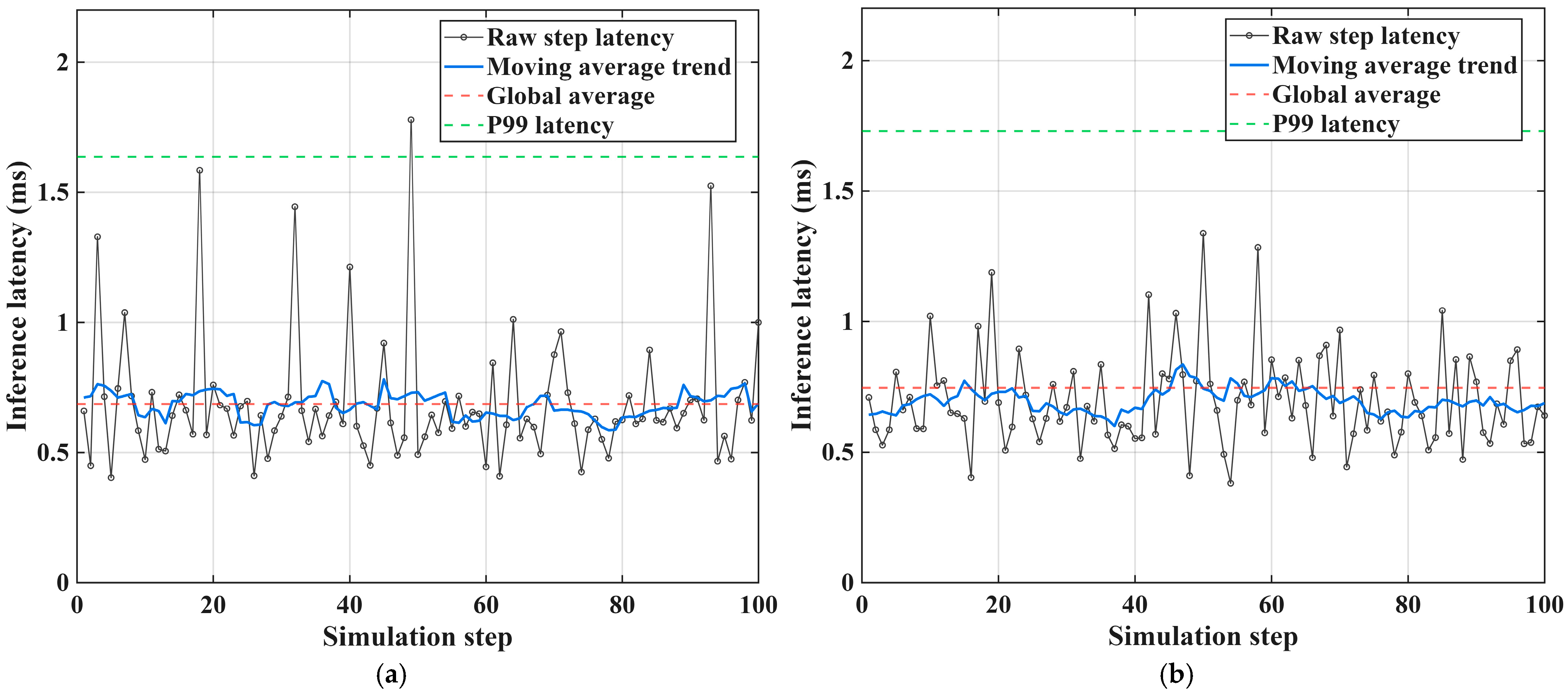
3.7. Computational Efficiency and Practical Implementation

To assess the feasibility of applying the proposed framework in wind-power forecasting systems, this section evaluates the computational cost and simulates a rolling forecasting process. The analysis separates the offline decomposition and optimization stages from the online prediction stage. ICEEMDAN, VMD, and CPO-based hyperparameter search are used for model preparation and are not repeatedly executed at each dispatch instant.

3.7.1. Computational Complexity Analysis

Table 8. Comparison of computational complexity and efficiency among forecasting models.

Model	Parameters (M)	Training Time (s/Epoch)	Inference Time (ms/Sample)
Informer	1.2840	0.6843	0.2386
Autoformer	1.5260	0.7925	0.2634
iTransformer	0.9360	0.5481	0.1912
CNN-BiLSTM	0.4120	0.2367	0.1185
Proposed Method	0.4380	0.2814	0.1268

summarizes the computational complexity of representative forecasting models in terms of trainable parameter count, training time, and inference time.

Regarding the signal-decomposition stage,

Table 9. Comparison of computational efficiency among decomposition strategies.

Algorithm	Processing Time (s/Day)	Overhead (ms/Sample)
VMD	1.8421	0.1184
CEEMDAN	5.9763	0.3842
ICEEMDAN	6.4138	0.4017
VMD-ICEEMDAN	6.9214	0.4365
CPO-ICEEMDAN-VMD	7.3846	0.4629

compares the execution efficiency of different decomposition strategies on a one-day wind-power window.

As shown in Table 8, the proposed method has a moderate parameter size of 0.4380 M because the online predictor is based on a CNN-BiLSTM component model rather than a full Transformer architecture. Its inference time is 0.1268 ms per sample, which is lower than the tested Transformer-based baselines and remains compatible with the forecasting setting considered in this study. For the signal decomposition shown in Table 9, the proposed CPO-ICEEMDAN-VMD strategy requires more processing time than a single VMD stage because it includes selective two-stage decomposition and offline parameter search. However, the average one-day processing time is 7.3846 s. Since this step is performed offline or during scheduled recalibration, the computational load is manageable for practical forecasting operations.

3.7.2. Real-Time Deployment Framework

To further examine practical feasibility, a real-time deployment simulation was conducted using a rolling forecasting mechanism on the test sets of the two external wind-power cases. The simulation imitates a dispatch scenario in which the system continuously receives data streams and performs point-by-point forecasting.

Table 10. Latency stability analysis of real-time rolling simulation.

Case	Test N	Avg. (ms)	Max (ms)	P99 (ms)	Occupancy (%)
Case 1	1151	0.6874	4.2800	1.6360	0.8210
Case 2	1151	0.7456	5.1700	1.7299	0.8211
Mean	/	0.7165	4.7250	1.6830	0.8210

summarizes the latency stability results, and Figure 16 visualizes the inference latency variations.

The data in Table 10 indicate that the average inference latency remains below 0.75 ms in both cases. The maximum latency does not exceed 5.17 ms, and the P99 latency remains below 1.73 ms. Even when the offline one-day decomposition preparation time is considered, the worst-case computational occupancy is approximately 0.8211% of the corresponding dispatch window, leaving a sufficient time margin for practical operation. Furthermore, as shown in Figure 16, the latency curves fluctuate around the average baseline without a sustained upward trend. This indicates that the online inference process does not show cumulative computational delay during the rolling forecasting procedure. Therefore, after offline preparation, the proposed framework can provide fast forecasting and serve as a reference for edge-computing or cloud-based deployment.

3.7.3. Zero-Generation and Deployment Interpretation

The proposed framework contains both offline model-preparation stages and online prediction stages. Feature screening, ICEEMDAN decomposition, sample-entropy grouping, VMD design, and CPO-based hyperparameter search are conducted during offline model training or scheduled recalibration. In contrast, the trained CNN-BiLSTM predictor is used for online inference. Therefore, the computationally heavier preprocessing and optimization procedures are not repeated at every dispatch instant.

In addition, the original wind-power sequence contains low-output and near-zero-generation intervals caused by low wind speed, turbine operating conditions, or possible maintenance-related shutdowns. These intervals were retained in both training and testing datasets rather than being removed as outliers. This treatment allows the reported performance metrics to reflect practical low-output operating conditions. Since the final fully connected layer uses a linear output before the regression layer, the model is not restricted by activation function saturation (such as sigmoid, tanh, or ReLU) at the final prediction stage. This structural design is suitable for continuous wind-power prediction, including near-zero values.

4. Conclusions

This paper proposes an ultra-short-term wind power forecasting method based on a hybrid CPO-ICEEMDAN-VMD-CNN-BiLSTM architecture. The method is designed to address the high nonlinearity, volatility, and non-stationarity of wind power series. By decomposing and reconstructing the wind power series using an adaptive ICEEMDAN-VMD strategy and utilizing a CNN-BiLSTM network for feature extraction and prediction, the framework aims to reduce forecasting errors and provide a data-driven reference for power system operation and renewable energy integration. The main conclusions are as follows:

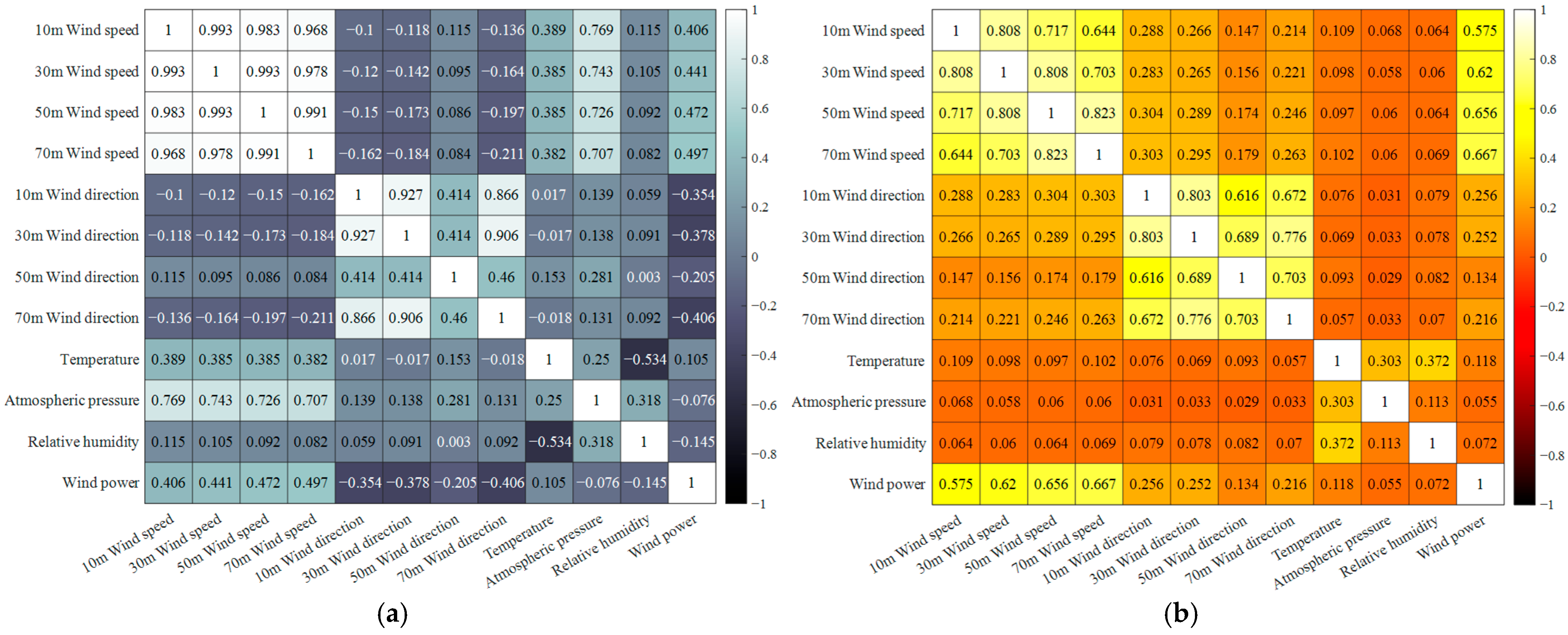
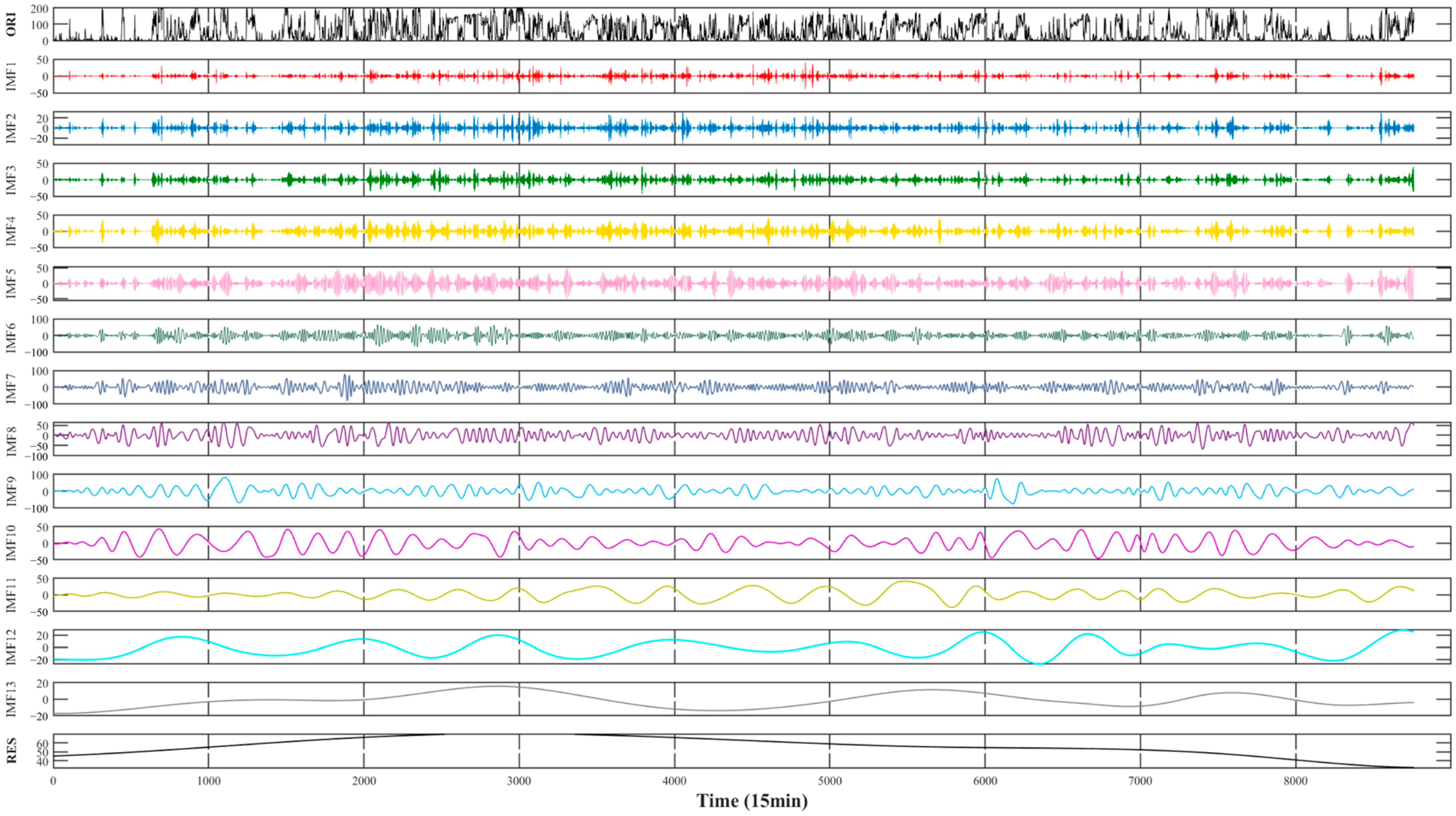
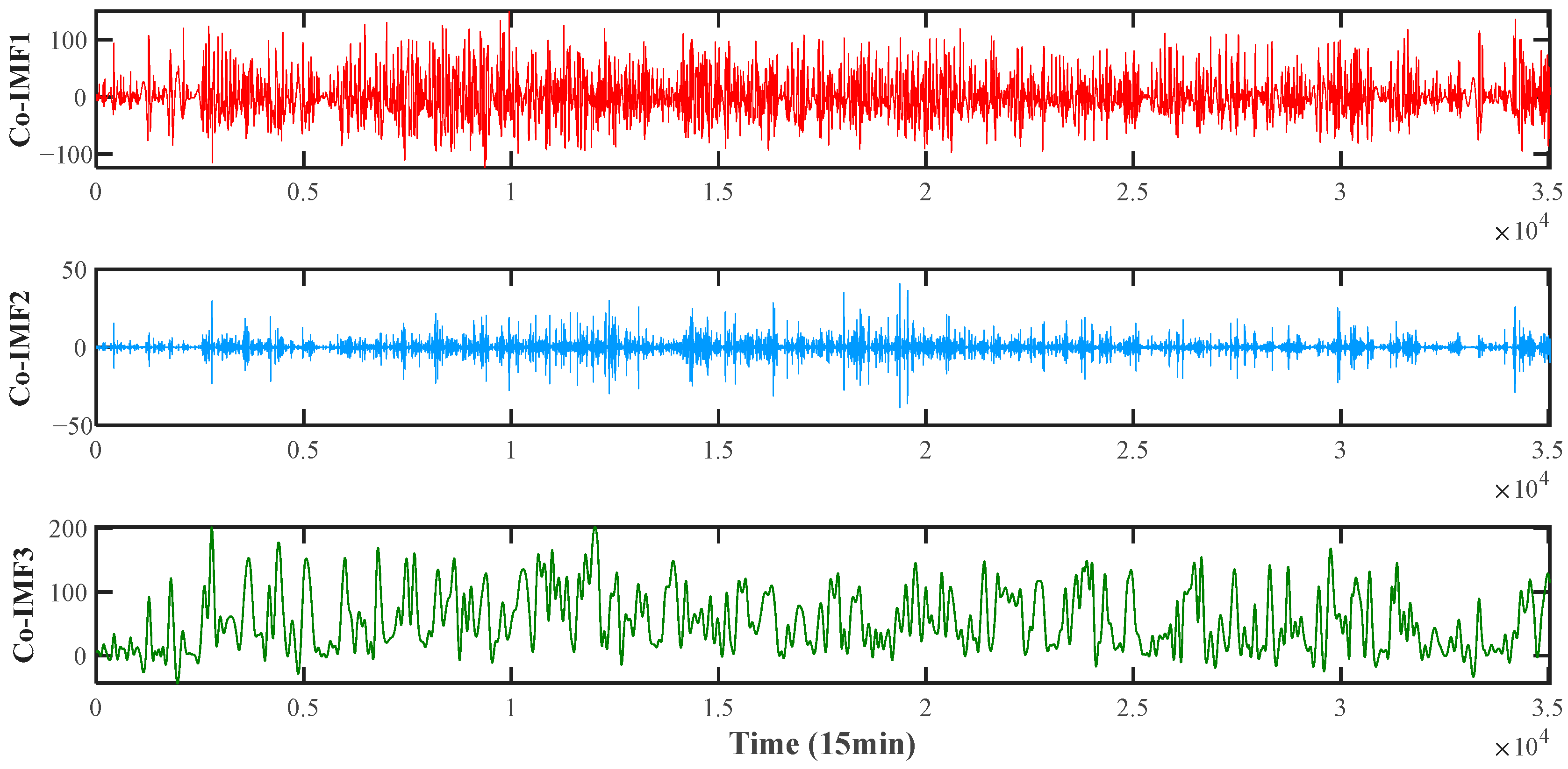
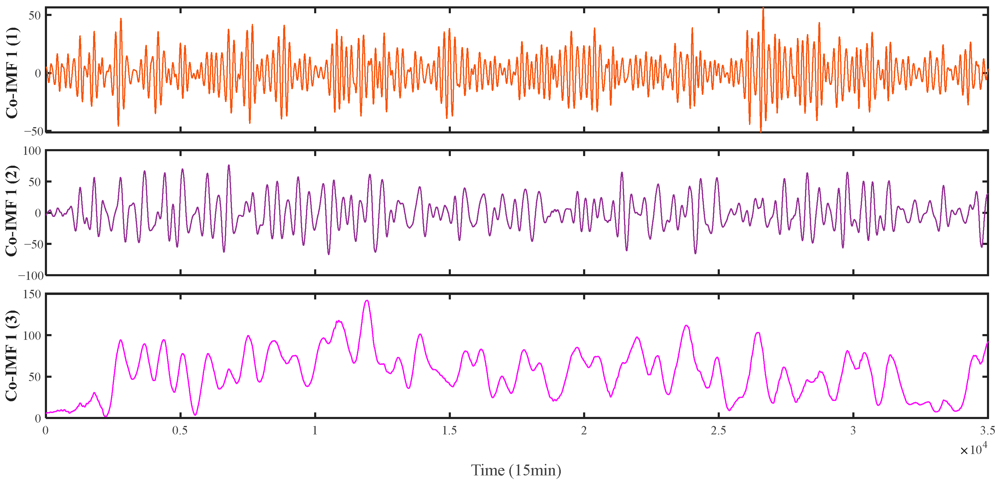
• Feature selection is performed using Pearson and MIC correlation coefficients to effectively reduce data dimensionality. The improved ICEEMDAN algorithm is employed for preliminary decomposition of the original wind power series, combined with sample entropy to quantify complexity and K-Means clustering to categorize IMF components into high, medium, and low frequency groups. VMD is applied exclusively to the high-frequency components for secondary decomposition, which extracts regular sub-modes and attenuates residual noise without over-decomposing the primary physical trend.
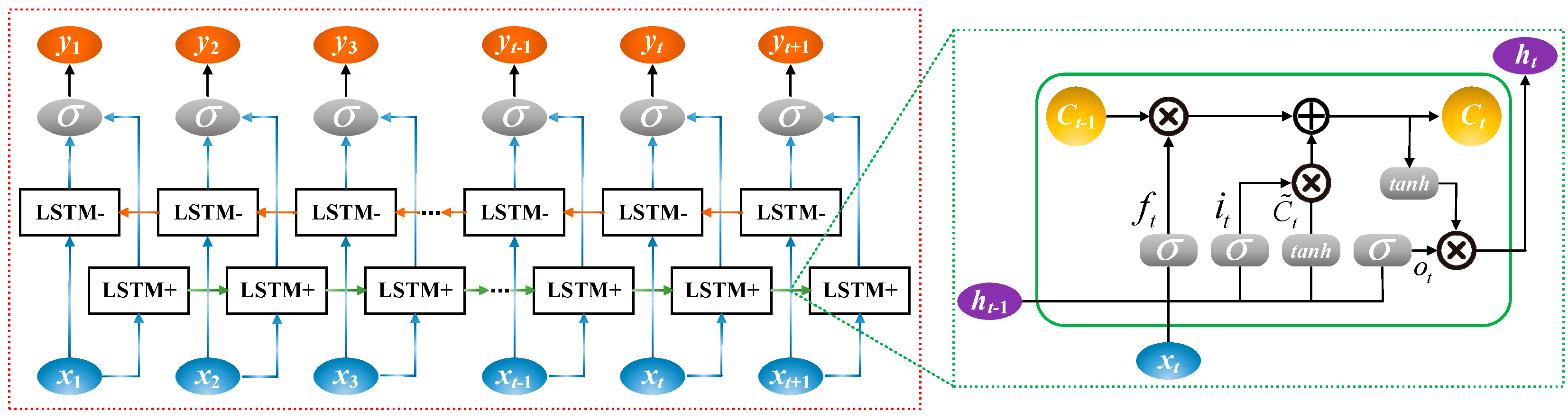
• The CNN module extracts local spatial features from the reconstructed modal components. The processed feature maps are then evaluated by the BiLSTM network to capture bidirectional temporal dependencies for the final continuous power prediction.
• The CPO algorithm adaptively optimizes key hyperparameters of the CNN-BiLSTM model, including the initial learning rate, regularization parameters, and hidden layer sizes. This automated configuration mechanism replaces empirical tuning and mathematically balances global exploration with local exploitation during the training phase.

Experimental results, including validations on independent external datasets across different seasonal scenarios, demonstrate that the proposed method yields lower prediction errors compared to basic deep learning models, single-decomposition variants, and recent Transformer-based architectures. Regarding practical operations, the forecasting precision of this architecture can assist grid operators in optimizing spinning reserve allocation, minimizing penalty costs in real-time balancing markets, and maintaining overall power system flexibility under varying generation conditions. In future research, advanced deep learning time-series forecasting architectures will be investigated, and automatic feature engineering techniques for handling extreme meteorological patterns will be explored to further validate the model’s transferability across diverse geographic environments.

References

- Lund, P.D.; Lindgren, J.; Mikkola, J.; Salpakari, J. Review of energy system flexibility measures to enable high levels of variable renewable electricity. Renew. Sustain. Energy Rev. 2015, 45, 785–807. [Google Scholar] [CrossRef] [Scilit]
- Shen, X.; Shen, J.; Wang, Y.; Wu, H. A deep reinforcement learning-based reactive power optimization method for distribution networks considering electric vehicle charging load prediction. Sustain. Energy Grids 2025, 43, 101777. [Google Scholar] [CrossRef] [Scilit]
- ENTSO-E. Final Report on the Grid Incident in Spain and Portugal on 28 April 2025; European Network of Transmission System Operators for Electricity (ENTSO-E): Brussels, Belgium, 2026; Available online: https://www.entsoe.eu/publications/blackout/28-april-2025-iberian-blackout/ (accessed on 7 June 2026).
- Shen, X.; Shen, J.; Zhang, T.; Zhang, Y.; Wang, Y. A two-stage framework for photovoltaic power forecasting: Integrating adaptive hybrid decomposition with a novel predictor. Eng. Appl. Artif. Intel. 2026, 174, 114469. [Google Scholar] [CrossRef] [Scilit]
- Zhang, J.; Cui, M.; Hodge, B.; Florita, A.; Freedman, J. Ramp forecasting performance from improved short-term wind power forecasting over multiple spatial and temporal scales. Energy 2017, 122, 528–541. [Google Scholar] [CrossRef] [Scilit]
- Wang, Y.; Pang, P.; Qi, B.; Wang, X.; Zhao, Z. A two-stage optimal pre-scheduling strategy for power system inertia assessment and replenishment under extreme weather events. Sustain. Comput.-Inform. 2025, 45, 101079. [Google Scholar] [CrossRef] [Scilit]
- Wang, Y.; Zhao, Z.; Qi, B.; Cheng, Y.; Tang, K.; Li, B. Vulnerability analysis of an electric vehicle fleet for car-sharing service under cyber attacks. Sustain. Energy Grids 2024, 37, 101207. [Google Scholar] [CrossRef] [Scilit]
- Li, J.; Zhang, S.; Yang, Z. A wind power forecasting method based on optimized decomposition prediction and error correction. Electr. Power Syst. Res. 2022, 208, 107886. [Google Scholar] [CrossRef] [Scilit]
- Abdollahi, A.; Samadi Gazijahani, F.; Alizadeh, A.; Taghizadegan Kalantari, N. Chance-constrained CAES and DRP scheduling to maximize wind power harvesting in congested transmission systems considering operational flexibility. Sustain. Cities Soc. 2019, 51, 101792. [Google Scholar] [CrossRef] [Scilit]
- Teleke, S.; Baran, M.E.; Bhattacharya, S.; Huang, A.Q. Optimal Control of Battery Energy Storage for Wind Farm Dispatching. IEEE Trans. Energy Conver. 2010, 25, 787–794. [Google Scholar] [CrossRef] [Scilit]
- He, X.; He, B.; Qin, T.; Lin, C.; Yang, J. Ultra-short-term wind power forecasting based on a dual-channel deep learning model with improved coot optimization algorithm. Energy 2024, 305, 132320. [Google Scholar] [CrossRef] [Scilit]
- Zhang, J.; Yan, J.; Infield, D.; Liu, Y.; Lien, F. Short-term forecasting and uncertainty analysis of wind turbine power based on long short-term memory network and Gaussian mixture model. Appl. Energy 2019, 241, 229–244. [Google Scholar] [CrossRef] [Scilit]
- Neshat, M.; Nezhad, M.M.; Abbasnejad, E.; Mirjalili, S.; Tjernberg, L.B.; Astiaso Garcia, D.; Alexander, B.; Wagner, M. A deep learning-based evolutionary model for short-term wind speed forecasting: A case study of the Lillgrund offshore wind farm. Energy Convers. Manag. 2021, 236, 114002. [Google Scholar] [CrossRef] [Scilit]
- Han, Q.; Meng, F.; Hu, T.; Chu, F. Non-parametric hybrid models for wind speed forecasting. Energy Convers. Manag. 2017, 148, 554–568. [Google Scholar] [CrossRef] [Scilit]
- Li, D.; Yu, X.; Liu, S.; Dong, X.; Zang, H.; Xu, R. Wind power prediction based on PSO-Kalman. Energy Rep. 2022, 8, 958–968. [Google Scholar] [CrossRef] [Scilit]
- Shi, J.; Teh, J.; Lai, C. Wind power prediction based on improved self-attention mechanism combined with Bi-directional Temporal Convolutional Network. Energy 2025, 322, 135666. [Google Scholar] [CrossRef] [Scilit]
- Wang, Y.; Zou, R.; Liu, F.; Zhang, L.; Liu, Q. A review of wind speed and wind power forecasting with deep neural networks. Appl. Energy 2021, 304, 117766. [Google Scholar] [CrossRef] [Scilit]
- Shahid, F.; Zameer, A.; Muneeb, M. A novel genetic LSTM model for wind power forecast. Energy 2021, 223, 120069. [Google Scholar] [CrossRef] [Scilit]
- Xiao, Y.; Zou, C.; Chi, H.; Fang, R. Boosted GRU model for short-term forecasting of wind power with feature-weighted principal component analysis. Energy 2023, 267, 126503. [Google Scholar] [CrossRef] [Scilit]
- Zhang, J.; Jiang, X.; Chen, X.; Li, X.; Guo, D.; Cui, L. Wind Power Generation Prediction Based on LSTM, New York, NY, USA, 2019-1-1; ACM: New York, NY, USA, 2019; pp. 85–89. [Google Scholar]
- Ko, M.S.; Lee, K.; Kim, J.K.; Hong, C.W.; Dong, Z.Y.; Hur, K. Deep Concatenated Residual Network with Bidirectional LSTM for One-Hour-Ahead Wind Power Forecasting. IEEE Trans. Sustain. Energy 2021, 12, 1321–1335. [Google Scholar] [CrossRef] [Scilit]
- Zhang, Y.; Wang, H. Multi-head attention-based probabilistic CNN-BiLSTM for day-ahead wind speed forecasting. Energy 2023, 278, 127865. [Google Scholar] [CrossRef] [Scilit]
- Liu, Y.; Dai, J.; Chen, G.; Cao, Q.; Jiang, F.; Wang, W. Integrating signal pairing evaluation metrics with deep learning for wind power forecasting through coupled multiple modal decomposition and aggregation. Knowl.-Based Syst. 2025, 317, 113394. [Google Scholar] [CrossRef] [Scilit]
- Sun, Q.; Che, J.; Hu, K.; Qin, W. Deterministic and probabilistic wind speed forecasting using decomposition methods: Accuracy and uncertainty. Renew. Energy 2025, 243, 122515. [Google Scholar] [CrossRef] [Scilit]
- Yu, Z.; Li, Y.; Du, X.; Liu, Y. Threshing cylinder unbalance detection using a signal extraction method based on parameter-adaptive variational mode decomposition. Biosyst. Eng. 2024, 244, 26–41. [Google Scholar] [CrossRef] [Scilit]
- Wang, J.; Zhang, W.; Li, Y.; Wang, J.; Dang, Z. Forecasting wind speed using empirical mode decomposition and Elman neural network. Appl. Soft Comput. 2014, 23, 452–459. [Google Scholar] [CrossRef] [Scilit]
- He, Y.; Wang, Y. Short-term wind power prediction based on EEMD–LASSO–QRNN model. Appl. Soft Comput. 2021, 105, 107288. [Google Scholar] [CrossRef] [Scilit]
- Lv, P.; Shu, Y.; Xu, J.; Wu, Q. Modal decomposition-based hybrid model for stock index prediction. Expert Syst. Appl. 2022, 202, 117252. [Google Scholar] [CrossRef] [Scilit]
- Han, L.; Jing, H.; Zhang, R.; Gao, Z. Wind power forecast based on improved Long Short Term Memory network. Energy 2019, 189, 116300. [Google Scholar] [CrossRef] [Scilit]
- Zeng, H.; Wu, B.; Fang, H.; Lin, J. Interpretable wind speed forecasting through two-stage decomposition with comprehensive relative importance analysis. Appl. Energy 2025, 392, 126015. [Google Scholar] [CrossRef] [Scilit]
- Shen, X.; Shen, J.; Zhang, Y.; Wu, H.; Wang, Y. A multi-source feature engineering-enhanced framework for mid-to-long-term EV charging load forecasting: Integrating self-adaptive optimization and BiLSTM-iTransformer predictor. Energy 2025, 339, 139020. [Google Scholar] [CrossRef] [Scilit]
- Abdel-Basset, M.; Mohamed, R.; Abouhawwash, M. Crested Porcupine Optimizer: A new nature-inspired metaheuristic. Knowl.-Based Syst. 2024, 284, 111257. [Google Scholar] [CrossRef] [Scilit]
- Fan, S.; Li, W.; Xie, R. Self-tuning trajectory tracking control for concrete pouring construction robots based on PID-NFTSMC and CPO algorithm. PLoS ONE 2025, 20, e0324550. [Google Scholar] [CrossRef] [Scilit] [PubMed]
- Shaheen, M.A.M.; Hasanien, H.M.; Mekhamer, S.F.; Talaat, H.E.A. Walrus optimizer-based optimal fractional order PID control for performance enhancement of offshore wind farms. Sci. Rep. 2024, 14, 17636. [Google Scholar] [CrossRef] [Scilit] [PubMed]
- Shaheen, M.A.M.; Hasanien, H.M.; Mekhamer, S.F.; Talaat, H.E.A. A chaos game optimization algorithm-based optimal control strategy for performance enhancement of offshore wind farms. Renew. Energy Focus 2024, 49, 100578. [Google Scholar] [CrossRef] [Scilit]
- Kennedy, J.; Eberhart, R. Particle swarm optimization. In Proceedings of the ICNN’95—International Conference on Neural Networks, Perth, WA, Australia, 27 November–1 December 1995; pp. 1942–1948. [Google Scholar]
- Mirjalili, S.; Lewis, A. The Whale Optimization Algorithm. Adv. Eng. Softw. 2016, 95, 51–67. [Google Scholar] [CrossRef] [Scilit]
- Mirjalili, S.; Mirjalili, S.M.; Lewis, A. Grey Wolf Optimizer. Adv. Eng. Softw. 2014, 69, 46–61. [Google Scholar] [CrossRef] [Scilit]
- Zhong, C.; Li, G.; Meng, Z. Beluga whale optimization: A novel nature-inspired metaheuristic algorithm. Knowl.-Based Syst. 2022, 251, 109215. [Google Scholar] [CrossRef] [Scilit]
- Su, H.; Zhao, D.; Heidari, A.A.; Liu, L.; Zhang, X.; Mafarja, M.; Chen, H. RIME: A physics-based optimization. Neurocomputing 2023, 532, 183–214. [Google Scholar] [CrossRef] [Scilit]
- Chen, Y.; Xu, J. Solar and wind power data from the Chinese State Grid Renewable Energy Generation Forecasting Competition. Sci. Data 2022, 9, 577. [Google Scholar] [CrossRef] [Scilit] [PubMed]
- Zhou, H.; Zhang, S.; Peng, J.; Zhang, S.; Li, J.; Xiong, H.; Zhang, W. Informer: Beyond Efficient Transformer for Long Sequence Time-Series Forecasting. In Proceedings of the AAAI Conference on Artificial Intelligence, Virtual Conference, 2–9 February 2021; AAAI Press: Palo Alto, CA, USA, 2021; Volume 35, pp. 11106–11115. [Google Scholar] [CrossRef] [Scilit]
- Wu, H.; Xu, J.; Wang, J.; Long, M. Autoformer: Decomposition Transformers with Auto-Correlation for Long-Term Series Forecasting. In Advances in Neural Information Processing Systems, Virtual Conference, 6–14 December 2021; Curran Associates, Inc.: Red Hook, NY, USA, 2021; Volume 34, pp. 22419–22430. [Google Scholar]
- Liu, Y.; Hu, T.; Zhang, H.; Wu, H.; Wang, S.; Ma, L.; Long, M. iTransformer: Inverted Transformers Are Effective for Time Series Forecasting. In Proceedings of the International Conference on Learning Representations, Vienna, Austria, 7–11 May 2024; OpenReview: London, UK, 2024. [Google Scholar]
- Diebold, F.X.; Mariano, R.S. Comparing Predictive Accuracy. J. Bus. Econ. Stat. 1995, 13, 253–263. [Google Scholar] [CrossRef] [Scilit]