Annual and Spatial Variation in the Diet of Juvenile Pacific Cod in Mutsu Bay, Japan

Abstract

To evaluate Mutsu Bay as a nursery habitat for Pacific cod (Gadus macrocephalus Tilesius, 1810), we analyzed settled age-0 juveniles collected with a small bottom otter trawl over 10 years. The three stations with the highest juvenile densities were targeted, and prey-specific feeding intensity (SCIi), its sum (SCI), and the relative condition factor (Kn) were quantified, followed by examining their relationships with juvenile attributes and environmental variables. Diets varied among stations and shifted ontogenetically from small-sized calanoid copepods to larger planktonic and benthic prey. SCI was highest at stations where juveniles consumed medium-sized plankton (0.1–1.0 mg ind⁻¹), including Calanus pacificus, Mesocalanus tenuicornis, Metridia pacifica, Anomura zoeae, and Euphausiacea furciliae, and lower where other prey dominated. High-SCI individuals were rarely observed, likely reflecting enhanced digestion at high temperatures near the upper habitat limit (~12 °C) and consistently low prey density independent of temperature. Kn increased with body size and SCI and tended to be higher in cooler water and closer to the bay mouth, suggesting coupled environmental and physiological constraints. These results suggest that after late May, juveniles may benefit from moving toward the bay mouth, where prey encounter rates are likely higher, including relatively larger prey, which may improve feeding opportunities and condition.

1. Introduction

The population dynamics of many fish species are strongly influenced by survival fluctuations during early life stages, including the egg, larval, and juvenile periods. Since Hjort’s critical period and transport hypotheses were proposed [1], numerous hypotheses have been advanced to explain recruitment variability. These include the match–mismatch hypothesis [2], the predation hypothesis [3,4], the growth and growth–predation hypotheses [5,6,7,8,9,10,11,12], the bigger-is-better hypothesis, and maternal effects [13,14,15,16]. Currently, no single hypothesis universally explains survival across species and populations; therefore, it is necessary to identify the factors influencing the survival for each species and population.

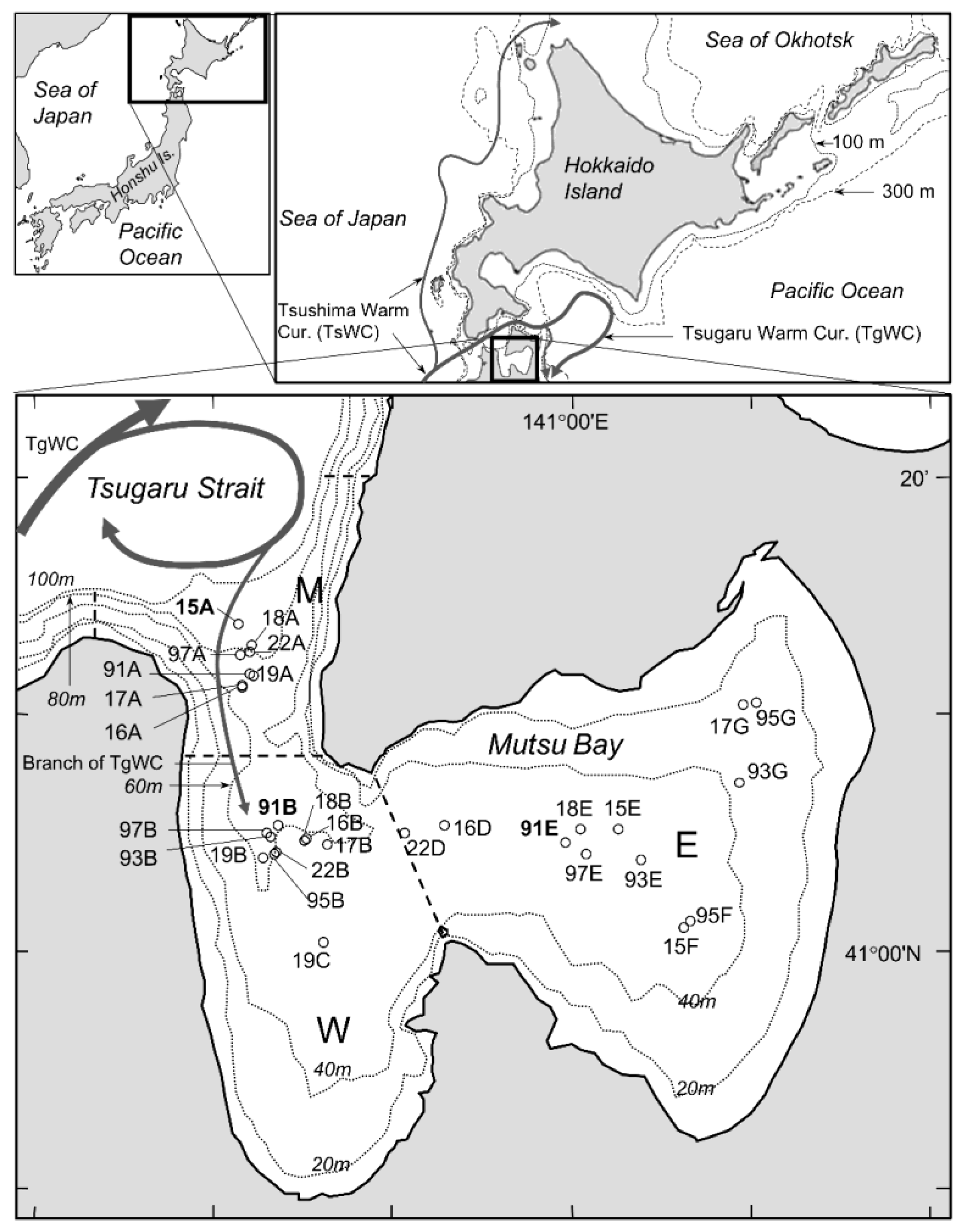
Pacific cod, Gadus macrocephalus Tilesius, 1810, is a cold-water demersal fish distributed across the continental shelf and slope of the North Pacific, from the Yellow Sea to the coast of California [17]. In Japan, it is harvested using various fishing methods in the Sea of Japan, the Sea of Okhotsk, and the Pacific Ocean off the northern part of Honshu and Hokkaido. Mutsu Bay is a major spawning ground for Pacific cod around Hokkaido Island and lies near the southern limit of their habitat in a relatively warm area [18] (Figure 1). From early December to mid-February, adults migrate into the bay from offshore depths of 100–300 m when water temperature in the bay and the bay mouth fall below 12 °C [19,20]. After hatching from demersal eggs, larvae ascend in the water column and are transported by a branch of the Tsugaru Warm Current (TgWC) [21] to the inner bay between February and March [18]. Large larvae and small juveniles are pelagic and occur at mid-water depths in April, while juveniles settle after late May [22]. Feeding habits shift with growth: first-feeding larvae (4.4–7.0 mm total length, TL) consume copepod nauplii; larger larvae (7–25 mm TL) and juveniles (26–70 mm TL) feed mainly on calanoid copepodites; and juveniles opportunistically feed on planktonic Gastropoda, Caridea (shrimp) zoeae, Brachyura (crab) megalopae, benthic Gammarida, and Pisces (fish) juveniles [23]. A survey from 1990 to 1997 revealed that survival rate variability was greater during the demersal juvenile stage (April–June) than that during larval and pelagic juvenile stages (February–April) [22,24]. In the eastern Bering Sea, pelagic age-0 Pacific cod primarily feed on large zooplankton and larval fishes, and the study demonstrated that climate-driven variation in prey quality strongly affects their energetic condition and potential overwinter survival [25]. In Alaska, demersal age-0 Pacific cod juveniles in coastal nurseries feed mainly on small Calanoida copepods, Mysidacea, and Gammarida, whereas shelf-associated juveniles may shift toward larger prey, particularly Euphausiacea, later in the growing season [26,27,28,29]. During marine heatwaves, juvenile diets shift toward greater reliance on mysids, and only a small number of large individuals may persist [29]. However, the relationship between the annual variation in feeding habits and nutritional condition during the settlement period (late May to June) in Mutsu Bay remains poorly understood. For many animals, food intake is the sole source of nutrition, and food quantity and quality strongly influence nutritional conditions and survival. Although extensive research has focused on feeding initiation in larvae, fewer studies have examined these relationships during the juvenile stage. While daily survival rates are generally higher in juveniles than in larvae, the juvenile stage lasts longer, making it unclear which stage contributes more to cumulative survival rate at recruitment [5].

In this study, the annual variation in feeding habits and nutritional condition of juvenile Pacific cod during settlement was examined to evaluate the roles of prey consumption, species, and size in population fluctuations. Specifically, we assessed daytime feeding to examine whether juveniles were able to secure sufficient food intensity, and we further investigated the prey taxa and body sizes that increased feeding levels. Further, we analyzed how juvenile body length, feeding intensity, and prey size in the stomach, together with water temperature and distance from the bay mouth, affected the nutritional condition of juveniles to identify key factors underlying the importance of this area as a nursery habitat for Pacific cod.

2. Materials and Methods

2.1. Overview of the Marine Environment of Mutsu Bay

The Tsugaru Strait connects the Sea of Japan to the west and the Pacific Ocean on the east (Figure 1). A part of the Tsushima Warm Current (TsWC) enters the strait, becomes the TgWC, and flows into the Pacific Ocean. The TgWC flows consistently from west to east, except during slack water at spring tide, which occurs once monthly [30]. North of the mouth of Mutsu Bay, part of the TgWC forms a clockwise eddy, while another part flows southward into the bay. The retention time of this water mass is approximately 1 month in the western bay (W; Figure 1) and 3 months in the eastern bay (E) [21]. Bottom water temperature in Mutsu Bay ranges annually from approximately 4–5 °C in March to 17–18 °C in October [21]. The maximum depths are 63 m in the western bay and 54 m in the eastern bay. Subarctic water exists in the deep layer beneath the TsWC in the Sea of Japan; consequently, cold-water zooplankton ascending from these deep layers are transported into the Mutsu Bay by the TgWC during the relatively cooler winter to spring months. As a result, cold-water and coastal planktons coexist within the bay.

2.2. Field Sampling

Samplings were conducted aboard the training ship T/S Ushio-maru (128 tons), Faculty of Fisheries, Hokkaido University, in Mutsu Bay from late May to early June in 2015–2019 and 2022 (

Table 1. The number of sampling stations and samples for Pacific cod Gadus macrocephalus juveniles collected by T/S Ushio-maru in Mutsu Bay, Japan. Data of 1991–1997 are quoted from Takatsu [22,24].

Dates	Number of Sampling Stations	Mean Density of Juveniles (10,000 inds. km−2) *
11–14 June 1991	5	12.22 ± 9.30
22–24 June 1993	6	0.79 ± 1.49
7–8 June 1995	6	4.51 ± 8.01
3–6 June 1997	7	6.77 ± 6.82
1–2 June 2015	8	0.21 ± 0.39
30 May–2 June 2016	8	5.86 ± 10.56
29 May–1 June 2017	8	52.3 ± 135.6
28–30 May 2018	8	190.8 ± 323.8
27–29 May 2019	8	31.7 ± 58.0
23–25 May 2022	8	57.8 ± 86.1

* ± standard deviation.

). Juveniles were collected using a small bottom otter trawl (4.4 m × 5.9 m mouth, 90 mm mesh, and 12 mm cod end mesh) [31] at eight stations. This trawl was towed along the seafloor for 5.3–31.3 min at approximately 1.5 m s⁻¹, as most Pacific cod juveniles had settled after late May [22]. Net contact with the seafloor was confirmed using an acoustic device attached to the net, and towing distance was measured using a standard Doppler device. Onboard, Pacific cod juveniles were already dead in almost all cases by the time they were brought onboard, were counted, and up to 300 individuals (all 298 individuals in 2015) were immediately fixed with 5–10% buffered formalin in seawater, then transferred to 70% ethanol after 24–36 h. The length shrinkage of juveniles due to fixation and preservation were not considered. Juvenile density (number of individuals per km²) at each sampling station was calculated from the net mouth width (5.9 m) and towing distance, assuming 100% filtration efficiency. Bottom water temperature 2 m above the seafloor at the sampling station (Tmp) was measured using a CTD.

Zooplankton were collected using vertical tows with flow meters, using two plankton nets of different diameters (45 cm in 1991–1997 and 80 cm in 2015–2022; both 0.335 mm mesh). Net mouth diameter varied among periods because of changes in survey objectives. Beginning in the 2000s, the net mouth diameter was expanded to 80 cm to increase filtered volume and thereby improve pelagic fish larvae collection, in addition to zooplankton. Data were missing at station 19A due to human error. Plankton samples were fixed onboard with 5% neutral formalin and later analyzed in the laboratory. No sampling was conducted to estimate the environmental densities of relatively larger-sized prey organisms (e.g., benthic Gammarida, Gastropoda, Polychaeta, Caridea juveniles, and Pisces juveniles).

2.3. Biological Measurements and Dietary Analyses

The TL of 20 juveniles from each of the three stations with the highest densities per year was measured to the nearest 0.01 mm using a digital caliper (Mitutoyo, Kawasaki, Japan) (except for station 15F in 2015, where only seven juveniles were collected). Their body weight (Bwt) and stomach-content weight (Scw) were measured to the nearest 0.001 g using an electronic balance (Mettler-Toledo, Greifensee, Switzerland).

Stomach contents were identified and counted under a stereomicroscope, with methylene blue staining used to detect appendicularians [32]. Frequently consumed calanoid copepods were identified at the species or genus level. Copepodite stages 2–5 (C2–C5) of Neocalanus plumchrus (Neo) were distinguished from N. flemingeri by the relative length of the second maxilla to prosome [33], and Metridia pacifica (Met), a species of calanoid copepods, was distinguished from M. lucens based on morphology [34]. The skeleton shrimp Caprella acanthogaster (Cap), present as plankton around Hokkaido Island during spring [35], was classified as plankton because the muddy seafloor in Mutsu Bay lacks suitable attachment substrates [22]. Prey items in the juvenile stomachs were dried on filter paper for 1–2 min and weighed to 0.1 mg using the same balance.

To evaluate feeding intensity, the stomach-content index, excluding digested materials (SCI, ‰), and prey-specific index (SCIi, ‰) were calculated using the following equations:

$${SCI}_i=1000·{Scw}_i/(Bwt-Scw)$$

(1)

$$SCI=\sum {SCI}_i$$

(2)

where Bwt, Scw, and Scw_i are body weight [g]; total stomach-content weight, including digested materials [g]; and the weight of prey item i [g], respectively. SCI represents the sum of SCIi and serves as an indicator of feeding intensity, excluding digested material. In this study, we considered prey weight in stomach contents to be the most relevant indicator of juvenile nutritional condition, rather than occurrence frequency or numerical composition. Furthermore, to account for differences in feeding intensity associated with individual body size, we used energy intake standardized by body weight. Compared with %W (mentioned later), SCI and SCIi reduce bias from individuals consuming unusually large prey because these indicies are standardized by predator body weight.

The mean prey weight for prey item i (Mpwp_i [mg ind⁻¹]) across all sampling stations was calculated using the following formula:

$${Mpwp}_i=\sum {Scw}_i/\sum n_i$$

(3)

where Scw_i is the stomach-content weight of prey item i [mg], and n_i is the number of individuals of prey item i observed in the stomach.

Mean prey weight per juvenile (Mpw_j [mg ind⁻¹]) at each station was calculated using the following formula:

$$Mpwj={\displaystyle {\sum }_{j=1}^m}\left({Scw}_j/n_j\right)/m$$

(4)

where Scw_j is the stomach-content weight [mg], excluding digested material; n_j is the total number of prey items in the stomach of juvenile, j; and m is the number of juveniles examined at the sampling station.

Stomach-content composition was also expressed as percent frequency of occurrence (%F, representing the percentage of juveniles that consumed a particular type of prey; Tables S1 and S4), numerical percent (%N, indicating the percentage of each prey type relative to the number of prey items; Tables S2 and S5), and weight percent (%W, indicating the percentage of each prey type relative to the weight of prey items; Tables S3 and S6). However, these metrics were not directly used in the analyses. Data from June surveys in 1991, 1993, 1995, and 1997 [24] (Table 2) were reanalyzed together with data from the years 2015–2019 and 2022. Specifically, the data from the 1990s were collected using the same vessel, sampling nets, towing procedures, and specimen preservation methods as in the present study. Data of Paracalanus parvus (1991–1997) were reclassified as P. orientalis following analyses conducted since 2015. Insects that came from land and sank from the sea surface in the stomach contents did not appear between 2015 and 2022 and were negligible (3.0 mg total, three individuals), and thus, they were excluded from this study. Prey items with %W ≤5% were grouped as other planktons (OPk: Bivalvia larvae, Cladocera, non-calanoid Copepoda, Euphausia pacifica calyptopis larvae, and Crustacean eggs) and other benthos (OBn: benthic Bivalvia, Oligocaeta, Monstrilloida, Cumacea, Isopoda, and Brachyura juveniles).

Table 2. Mean stomach-content weight index for prey item i (SCIi; ‰) of Pacific cod G. macrocephalus juveniles by sampling station in Mutsu Bay, Japan, in 1991, 1993, 1995, and 1997. Original data are quoted from Takatsu [24]. Prey taxa are arranged in ascending order of mean prey weight (Mpwp; Table 3) observed in stomach contents. The attributes of juveniles used for stomach-content analysis are also provided.

Sampling Year		1991			1993			1995			1997
Prey Items/Sampling Station	Abb. name	Stn.A	Stn.B	Stn.E	Stn.B	Stn.E	Stn.G	Stn.B	Stn.F	Stn.G	Stn.A	Stn.B	Stn.E
Other planktonic items	OPk	0	0.14	0.38	0.18	0.52	0	0	0.62	0	0	0	0.13
Appendicularia	Apn	0	0	0	0	0	0	0	0	0	0	0	0
Small-sized Calanoida (<0.1 mg ind−1)	CaS	0	1.72	6.40	0.41	3.77	0.77	1.92	2.92	1.35	0	0.05	0.09
Gastropoda larva	GaL	0	0	0	0	0	0	0	10.86	0	0	0	0.26
Metridia pacifica	Met	0	0.03	0	0	0	0	0	0	0	0.00	0	0
Brachyura (crab) zoea	BrZ	0	0	0.03	0.30	0.03	0.05	0	0.03	0	0.13	0.03	0
Euphausiacea furcilia	EuF	0.02	3.07	0.03	0.46	0	0	0	0.05	0	0.17	0	0
Medium-sized Calanoida (0.1–1.0 mg ind−1)	CaM	0.02	5.12	2.38	10.48	0.80	6.06	0.10	0.03	0.30	0.23	0	0.03
Anomura zoea	AnZ	0	0	0.03	0	0	0	0	0	0.15	0.04	0	0
Pisces (fish) egg and larva	PEL	0	0	0	0.04	0.03	0.05	0.10	0	0	0	0	0
Caridea (shrimp) zoea	CrZ	0.06	0.29	0	0.05	1.01	4.35	0.02	0	0.05	0	0.46	0.09
Sagittoidea	Sag	0.11	0	0	1.10	0	0	0	0.28	0	0	0.51	0
Hyperiidea	Hyp	0	0	0	0.06	0	0	0.11	0	0	1.69	0.73	0.02
Polychaeta larva	PoL	0	0	0	0	0	0	0	0.09	0.10	0	0	0.25
Ostracoda	Ost	0	0	0	0	0	0	0	0	0	0	0	0
Other benthos	OBn	0.05	0.16	0.07	0	0	0.06	0	0	0	0.50	1.00	0.20
Neocalanus plumchrus	Neo	0	0	0	0	0	0	0	0	0	0	0.03	0.05
Caprella acanthogaster (plankton)	Cap	0	0.07	0	0.32	0.23	0	0	0	0.88	0	2.96	0.70
Annomura megalopa	AnM	0	0	0	0	0	0	0.07	0	0	0.46	2.97	0.58
Gammarida (benthos)	Gam	0.11	0	0	0	0.07	0	0.42	0.08	0.06	1.10	0.99	0.01
Brachyura (crab) megalopa	BrM	0	0	0.02	0	0	0.07	0.64	0	0.65	0	3.00	1.64
Gastropoda (benthos)	GaB	0	0	0	0	0	0	0	0	0	0	0.89	0
Polychaeta (benthos)	PoB	0	0	0	0	0	0	0	0	0	0	0.32	0
Caridea (shrimp) juvenile	CrJ	0.43	0	0	0.92	0	0	0.26	0	0.31	0.76	1.15	0
Pisces (fish) juvenile	PJv	0	0	0	0	0.09	0	0.07	0	1.53	0.22	0.34	0
Sample size of juvenile stomachs		20	20	20	22	20	13	20	20	20	32	30	32
Mean total length of juveniles (TL; mm)		72.48	66.80	68.79	69.02	66.04	72.56	64.54	59.30	73.75	61.92	65.44	66.74
Minimum total length of juveniles (TL; mm)		65.48	52.74	55.48	56.39	56.70	66.86	45.48	41.59	57.64	38.69	47.35	49.70
Maximum total length of juveniles (TL; mm)		81.38	78.01	81.48	84.31	84.69	86.09	92.85	82.42	92.56	86.70	82.88	90.21
Mean body weight of juveniles [g]		2.15	1.95	1.91	1.99	1.66	2.10	1.09	1.26	2.36	1.64	1.57	1.75
Mean stomach contents weight (Scw; mg) *		3.15	22.1	26.8	30.9	12.3	25.5	4.8	14.8	18.9	7.5	31.4	20.8
Mean stomach contents index (SCI; ‰)		0.79	10.62	9.33	14.33	6.55	11.40	3.71	14.97	5.38	5.30	15.43	4.05
Mean number of prey (number of prey ind.)		4.85	95.8	218.8	86.9	117.6	78.5	36.2	246.2	35.0	4.91	11.0	13.9
Mean prey weight for juvenile (Mpwj; mg ind−1)		1.498	0.189	0.089	0.386	0.218	0.369	0.143	0.089	1.804	4.073	4.000	2.719
Mean relative condition factor (Kn) **		2.03	2.26	2.40	2.18	2.04	1.86	1.94	2.25	1.97	2.10	2.21	2.08
Juvenile density (JuvDens; 10,000 ind km−2)		13.71	28.71	11.42	4.12	0.28	0.18	1.31	1.93	22.37	9.74	6.80	21.71
Water temperature near bottom (Tmp; °C)		9.06	8.91	7.79	10.79	10.43	11.64	10.51	9.61	8.92	10.11	9.91	9.79
Bottom depth (m)		75	61	48	59	44	36	58	42	30	78	60	49
Distance from Stn.15A (nm)		2.27	8.61	20.99	9.09	24.33	28.87	9.81	27.31	31.03	1.27	8.92	21.93

“0” indicates 0, and “0.00” indicates a per mille of less than 0.005; * inclusive of digested materials. ** Kn = (body weight [g]—stomach contents weight [g])/total length [mm]^3.533.

Table 2. Mean stomach-content weight index for prey item i (SCIi; ‰) of Pacific cod G. macrocephalus juveniles by sampling station in Mutsu Bay, Japan, in 1991, 1993, 1995, and 1997. Original data are quoted from Takatsu [24]. Prey taxa are arranged in ascending order of mean prey weight (Mpwp; Table 3) observed in stomach contents. The attributes of juveniles used for stomach-content analysis are also provided.

Sampling Year		1991			1993			1995			1997
Prey Items/Sampling Station	Abb. name	Stn.A	Stn.B	Stn.E	Stn.B	Stn.E	Stn.G	Stn.B	Stn.F	Stn.G	Stn.A	Stn.B	Stn.E
Other planktonic items	OPk	0	0.14	0.38	0.18	0.52	0	0	0.62	0	0	0	0.13
Appendicularia	Apn	0	0	0	0	0	0	0	0	0	0	0	0
Small-sized Calanoida (<0.1 mg ind−1)	CaS	0	1.72	6.40	0.41	3.77	0.77	1.92	2.92	1.35	0	0.05	0.09
Gastropoda larva	GaL	0	0	0	0	0	0	0	10.86	0	0	0	0.26
Metridia pacifica	Met	0	0.03	0	0	0	0	0	0	0	0.00	0	0
Brachyura (crab) zoea	BrZ	0	0	0.03	0.30	0.03	0.05	0	0.03	0	0.13	0.03	0
Euphausiacea furcilia	EuF	0.02	3.07	0.03	0.46	0	0	0	0.05	0	0.17	0	0
Medium-sized Calanoida (0.1–1.0 mg ind−1)	CaM	0.02	5.12	2.38	10.48	0.80	6.06	0.10	0.03	0.30	0.23	0	0.03
Anomura zoea	AnZ	0	0	0.03	0	0	0	0	0	0.15	0.04	0	0
Pisces (fish) egg and larva	PEL	0	0	0	0.04	0.03	0.05	0.10	0	0	0	0	0
Caridea (shrimp) zoea	CrZ	0.06	0.29	0	0.05	1.01	4.35	0.02	0	0.05	0	0.46	0.09
Sagittoidea	Sag	0.11	0	0	1.10	0	0	0	0.28	0	0	0.51	0
Hyperiidea	Hyp	0	0	0	0.06	0	0	0.11	0	0	1.69	0.73	0.02
Polychaeta larva	PoL	0	0	0	0	0	0	0	0.09	0.10	0	0	0.25
Ostracoda	Ost	0	0	0	0	0	0	0	0	0	0	0	0
Other benthos	OBn	0.05	0.16	0.07	0	0	0.06	0	0	0	0.50	1.00	0.20
Neocalanus plumchrus	Neo	0	0	0	0	0	0	0	0	0	0	0.03	0.05
Caprella acanthogaster (plankton)	Cap	0	0.07	0	0.32	0.23	0	0	0	0.88	0	2.96	0.70
Annomura megalopa	AnM	0	0	0	0	0	0	0.07	0	0	0.46	2.97	0.58
Gammarida (benthos)	Gam	0.11	0	0	0	0.07	0	0.42	0.08	0.06	1.10	0.99	0.01
Brachyura (crab) megalopa	BrM	0	0	0.02	0	0	0.07	0.64	0	0.65	0	3.00	1.64
Gastropoda (benthos)	GaB	0	0	0	0	0	0	0	0	0	0	0.89	0
Polychaeta (benthos)	PoB	0	0	0	0	0	0	0	0	0	0	0.32	0
Caridea (shrimp) juvenile	CrJ	0.43	0	0	0.92	0	0	0.26	0	0.31	0.76	1.15	0
Pisces (fish) juvenile	PJv	0	0	0	0	0.09	0	0.07	0	1.53	0.22	0.34	0
Sample size of juvenile stomachs		20	20	20	22	20	13	20	20	20	32	30	32
Mean total length of juveniles (TL; mm)		72.48	66.80	68.79	69.02	66.04	72.56	64.54	59.30	73.75	61.92	65.44	66.74
Minimum total length of juveniles (TL; mm)		65.48	52.74	55.48	56.39	56.70	66.86	45.48	41.59	57.64	38.69	47.35	49.70
Maximum total length of juveniles (TL; mm)		81.38	78.01	81.48	84.31	84.69	86.09	92.85	82.42	92.56	86.70	82.88	90.21
Mean body weight of juveniles [g]		2.15	1.95	1.91	1.99	1.66	2.10	1.09	1.26	2.36	1.64	1.57	1.75
Mean stomach contents weight (Scw; mg) *		3.15	22.1	26.8	30.9	12.3	25.5	4.8	14.8	18.9	7.5	31.4	20.8
Mean stomach contents index (SCI; ‰)		0.79	10.62	9.33	14.33	6.55	11.40	3.71	14.97	5.38	5.30	15.43	4.05
Mean number of prey (number of prey ind.)		4.85	95.8	218.8	86.9	117.6	78.5	36.2	246.2	35.0	4.91	11.0	13.9
Mean prey weight for juvenile (Mpwj; mg ind−1)		1.498	0.189	0.089	0.386	0.218	0.369	0.143	0.089	1.804	4.073	4.000	2.719
Mean relative condition factor (Kn) **		2.03	2.26	2.40	2.18	2.04	1.86	1.94	2.25	1.97	2.10	2.21	2.08
Juvenile density (JuvDens; 10,000 ind km−2)		13.71	28.71	11.42	4.12	0.28	0.18	1.31	1.93	22.37	9.74	6.80	21.71
Water temperature near bottom (Tmp; °C)		9.06	8.91	7.79	10.79	10.43	11.64	10.51	9.61	8.92	10.11	9.91	9.79
Bottom depth (m)		75	61	48	59	44	36	58	42	30	78	60	49
Distance from Stn.15A (nm)		2.27	8.61	20.99	9.09	24.33	28.87	9.81	27.31	31.03	1.27	8.92	21.93

“0” indicates 0, and “0.00” indicates a per mille of less than 0.005; * inclusive of digested materials. ** Kn = (body weight [g]—stomach contents weight [g])/total length [mm]^3.533.

Table 3. Mean prey weight by prey item (Mpwp; mg ind⁻¹) in the stomach contents of Pacific cod G. macrocephalus juveniles in Mutsu Bay.

Prey Items	Abb. Name	Mpwp ± Standard Deviation (mg ind−1)	n
Other planktonic items	OPk	0.017 ± 0.109	371
Appendicularia	Apn	0.050 ± 0.069	82
Small-sized Calanoida (<0.1 mg ind−1)	CaS *	0.083 ± 0.081	540
Gastropoda larva	GaL *	0.174 ± 0.461	77
Metridia pacifica	Met *	0.187 ± 0.230	73
Brachyura (crab) zoea	BrZ *	0.211 ± 0.382	65
Euphausiacea furcilia	EuF *	0.242 ± 0.364	135
Medium-sized Calanoida (0.1–1.0 mg ind−1)	CaM *	0.246 ± 0.231	154
Anomura zoea	AnZ *	0.37 ± 0.43	71
Pisces (fish) egg and larva	PEL	0.38 ± 0.45	11
Caridea (shrimp) zoea	CrZ *	0.42 ± 0.53	127
Sagittoidea	Sag *	0.45 ± 0.72	79
Hyperiidea	Hyp	0.546 ± 0.85	109
Polychaeta larva	PoL	0.549 ± 1.97	26
Ostracoda	Ost	0.83 ± 0.57	4
Other benthos	OBn	1.13 ± 1.60	33
Neocalanus plumchrus	Neo *	1.24 ± 0.60	53
Caprella acanthogaster (plankton)	Cap *	1.49 ± 2.63	169
Annomura megalopa	AnM	2.13 ± 1.99	38
Gammarida (benthos)	Gam	2.19 ± 2.45	50
Brachyura (crab) megalopa	BrM	3.97 ± 4.56	55
Gastropoda (benthos)	GaB	4.50 ± 3.42	4
Polychaeta (benthos)	PoB	5.14 ± 8.96	8
Caridea (shrimp) juvenile	CrJ	16.44 ± 28.65	19
Pisces (fish) juvenile	PJv	35.92 ± 89.12	12

* Environmental densities of 11 plankton taxa were estimated from plankton-net samples (Figure 9).

Table 3. Mean prey weight by prey item (Mpwp; mg ind⁻¹) in the stomach contents of Pacific cod G. macrocephalus juveniles in Mutsu Bay.

Prey Items	Abb. Name	Mpwp ± Standard Deviation (mg ind−1)	n
Other planktonic items	OPk	0.017 ± 0.109	371
Appendicularia	Apn	0.050 ± 0.069	82
Small-sized Calanoida (<0.1 mg ind−1)	CaS *	0.083 ± 0.081	540
Gastropoda larva	GaL *	0.174 ± 0.461	77
Metridia pacifica	Met *	0.187 ± 0.230	73
Brachyura (crab) zoea	BrZ *	0.211 ± 0.382	65
Euphausiacea furcilia	EuF *	0.242 ± 0.364	135
Medium-sized Calanoida (0.1–1.0 mg ind−1)	CaM *	0.246 ± 0.231	154
Anomura zoea	AnZ *	0.37 ± 0.43	71
Pisces (fish) egg and larva	PEL	0.38 ± 0.45	11
Caridea (shrimp) zoea	CrZ *	0.42 ± 0.53	127
Sagittoidea	Sag *	0.45 ± 0.72	79
Hyperiidea	Hyp	0.546 ± 0.85	109
Polychaeta larva	PoL	0.549 ± 1.97	26
Ostracoda	Ost	0.83 ± 0.57	4
Other benthos	OBn	1.13 ± 1.60	33
Neocalanus plumchrus	Neo *	1.24 ± 0.60	53
Caprella acanthogaster (plankton)	Cap *	1.49 ± 2.63	169
Annomura megalopa	AnM	2.13 ± 1.99	38
Gammarida (benthos)	Gam	2.19 ± 2.45	50
Brachyura (crab) megalopa	BrM	3.97 ± 4.56	55
Gastropoda (benthos)	GaB	4.50 ± 3.42	4
Polychaeta (benthos)	PoB	5.14 ± 8.96	8
Caridea (shrimp) juvenile	CrJ	16.44 ± 28.65	19
Pisces (fish) juvenile	PJv	35.92 ± 89.12	12

* Environmental densities of 11 plankton taxa were estimated from plankton-net samples (Figure 9).

To evaluate the nutritional condition of cod juveniles, the relative condition factor (Kn) was calculated using the following equation:

Kn = (Bwt − Scw)/TL^b

(5)

where b is a coefficient specific to this paper, and TL is total length [mm]. The coefficient b is 3.532, estimated from the allometric equation estimated for the relationship between TL and (Bwt–Scw) of all juveniles used in this study (log(Bwt − Scw)) = 3.532 log(TL) − 6.22 (r² = 0.974, n = 825). Kn is the deviation from the mean weight–length relationship [36] and reduces size-related bias compared with Fulton’s K (b = 3).

2.4. Data Analysis

Water temperature 2 m above the seafloor (Tmp [°C]), mean TL of juveniles (TL [mm]), relative condition factor (Kn), and horizontal distance from station 15A at the bay mouth (Dist [nautical miles]) were used as explanatory variables in subsequent statistical analyses (Table 2 and

Table 4. Mean stomach-content weight index for prey item i (SCIi; ‰) of Pacific cod G. macrocephalus juveniles by sampling station in Mutsu Bay (2015–2019 and 2022). The prey taxa are arranged in ascending order of mean prey weight (Mpwp; Table 3) observed in the stomach contents. The attributes of juveniles used for stomach-content analysis are also provided.

Sampling Year		2015			2016			2017			2018			2019			2022
Prey Items/Sampling Station	Abb. Name	Stn.A	Stn.E	Stn.F	Stn.A	Stn.B	Stn.D	Stn.A	Stn.B	Stn.G	Stn.A	Stn.B	Stn.E	Stn.A	Stn.B	Stn.C	Stn.A	Stn.B	Stn.D
Other planktonic items	OPk	0.13	0.00	0.0	0.0	0.00	0.01	0.01	0.08	0.07	0.06	0.04	0.01	0.02	0.14	0.00	0.08	0.02	0.00
Appendicularia	Apn	0.09	0.04	0.0	0.02	0.00	0.00	2.51	0	0.0	0.57	0.11	0.98	0.11	0.00	0	0.03	0.00	0.00
Small-sized Calanoida (<0.1 mg ind−1)	CaS	0.32	10.78	7.77	0.07	2.81	4.61	1.62	2.22	6.36	0.85	0.05	5.28	0.97	7.67	5.72	4.02	5.49	8.32
Gastropoda larva	GaL	0.00	0	0	0.01	0	0	0.03	0	0	0.18	0	0.36	0.04	0	0	0.08	0	0
Metridia pacifica	Met	0.04	0.00	0	29.79	0.08	0	5.58	0	0	0.59	0.07	0.03	0.10	0.00	0	0.07	0	0
Brachyura (crab) zoea	BrZ	0	0	0	0.01	0	0.01	0	0	0	0.01	0	0	0.57	0	0	0.00	0	0
Euphausiacea furcilia	EuF	0.01	0.10	0	0.65	0	0.14	0.02	0.55	0.19	0.39	0.00	0.38	0.44	0.11	0.01	0.21	0.02	0
Medium-sized Calanoida (0.1–1.0 mg ind−1)	CaM	0.11	0.80	0.11	2.46	0.01	0.04	0.09	0.20	2.03	1.66	0	1.55	0.13	0.08	0.05	0.77	0.01	0
Anomura zoea	AnZ	0.02	0.00	0	12.27	0.12	0.02	0	0.30	0	7.69	0.09	0.15	0.40	0.10	0	0.06	0.02	0
Pisces (fish) egg and larva	PEL	0.02	0.01	0	0	0	0	0	0	0	0	0	0	0	0	0	0.02	0	0
Caridea (shrimp) zoea	CrZ	0	0.19	0.29	2.03	0.03	0.34	0	0.04	0.01	0.17	0	0.00	0.20	0.02	0.06	0.02	0.01	0.04
Sagittoidea	Sag	0	0.59	0	1.53	0.03	0.02	0	0	0	0.46	0	2.92	0	0	0	0.03	0	0
Hyperiidea	Hyp	0	0.00	0	2.29	0.05	0.09	0.87	0	0.05	1.76	0.02	0.14	1.61	0.65	0.01	0.05	0	0
Polychaeta larva	PoL	0	0.00	0	0.01	0	0	0	0.12	0	0	0	0	0.00	0	0	0.01	0	0
Ostracoda	Ost	0.20	0	0	0.01	0	0	0	0	0	0	0	0	0	0	0	0	0	0
Other benthos	OBn	0.04	0	0	0.00	0	0	0.01	0	0	0	0	0	0	0	0	0	0	0
Neocalanus plumchrus	Neo	0	0	0	0.29	0	0	0.11	0	1.05	0.63	10.84	3.79	0.06	0	0	0	0	0
Caprella acanthogaster (plankton)	Cap	0.06	0.07	0.21	0.18	2.26	2.69	0	0.15	0	1.21	0	0.96	0	0.14	0.01	0.26	0.61	0.82
Annomura megalopa	AnM	0.05	0	0	0.20	0.00	0	0.14	0.11	0	0.16	0.08	0	0.07	0	0	0	0	0
Gammarida (benthos)	Gam	0	0	0	0.11	0.01	0	0.29	0	0.16	0.06	0	0	0.44	0	0	0.01	0	0
Brachyura (crab) megalopa	BrM	0	0.04	0	0	0	0.3	0	0.18	0	0	0	0	1.06	0	0	0	0	0
Gastropoda (benthos)	GaB	0	0	0	0	0	0	0	0	0	0	0	0	0	0	0	0.09	0	0
Polychaeta (benthos)	PoB	0	0	0	0	0	1.1	0	0	0	0	0	0	0	0	0	0	0	0
Caridea (shrimp) juvenile	CrJ	0.02	0	0	0	0	0	0	0	0	0.30	0	0	0	0	0	0	0	0
Pisces (fish) juvenile	PJv	0	0	0	1.84	0	0	0	0	0	0	0	0	0	0	0	0	0	0
Sample size of juvenile stomachs		20	20	7	20	20	20	20	20	20	20	20	20	20	20	20	20	20	20
Mean total length of juveniles (TL; mm)		58.52	63.67	58.39	57.22	55.53	61.61	60.80	56.74	59.19	56.82	59.28	56.77	47.30	50.52	45.63	46.13	44.31	40.88
Minimum total length of juveniles (TL; mm)		50.22	56.23	45.76	46.06	42.56	49.24	50.83	43.77	47.59	48.21	49.20	46.53	34.36	39.60	39.21	37.74	38.73	35.86
Maximum total length of juveniles (TL; mm)		67.55	70.42	64.26	87.15	69.19	84.42	66.85	70.11	75.78	65.87	74.43	75.00	56.46	56.35	49.54	54.97	53.06	43.78
Mean body weight of juveniles [g]		1.06	1.44	1.17	1.29	0.83	1.28	1.24	1.02	1.00	1.10	1.29	1.06	0.48	0.62	0.40	0.42	0.39	0.28
Mean stomach contents weight (Scw; mg) *		2.84	20.31	12.17	54.56	7.50	12.73	16.38	5.53	10.03	22.23	14.50	16.85	4.73	5.46	2.80	3.10	2.53	3.41
Mean stomach contents index (SCI; ‰)		1.12	12.63	8.38	53.76	5.39	9.38	11.28	3.95	9.92	16.74	11.31	16.56	6.20	8.91	5.86	5.80	6.17	9.19
Mean number of prey (number of prey ind.)		11.75	174.0	191.6	180.5	48.5	86.2	76.45	33.5	146.8	57.65	14.55	68.8	21.2	86.0	49.3	60.7	64.2	72.8
Mean prey weight for juvenile (Mpwj; mg ind−1)		0.132	0.099	0.050	0.533	0.473	1.329	0.266	0.223	0.126	0.564	0.821	0.434	0.329	0.077	0.047	0.039	0.033	0.034
Mean relative condition facor (Kn) **		1.97	2.05	2.21	2.35	1.87	1.89	2.09	2.13	1.80	2.31	2.32	2.16	1.90	2.00	1.89	1.81	1.98	1.90
Juvenile density (JuvDens; 10,000 ind km−2)		1.22	0.26	0.08	33.2	5.5	5.3	411.0	2.1	2.1	220.3	1030.2	117.0	15.5	183.8	26.7	272.1	43.9	97.3
Water temperature near bottom (Tmp; °C)		10.19	9.54	10.61	10.16	9.68	11.56	10.37	9.98	10.49	10.15	9.93	9.37	9.57	9.80	10.77	9.87	8.88	8.39
Bottom depth (m)		91	46	43	73	59	52	70	58	32	80	57	47	73	60	52	77	58	53
Distance from Stn.15A (nm)		0	23.20	27.29	2.67	9.57	15.77	2.59	10.10	30.54	1.05	9.58	21.63	2.20	9.98	13.98	1.31	9.79	14.10

“0” indicates 0, and “0.00” indicates a per mille of <0.005; * inclusive of digested materials; ** Kn = (body weight [g]—stomach contents weight [g])/total length [mm]^3.533.

). Dist was calculated as follows: for stations A and B, straight-line distance from 15A—the outermost station; 91 m in depth (Figure 1)—was used; for stations C, D, and E, distance via 91B was used; and for stations F and G, distance via both 91B and 91E was used. All routes followed the deepest possible paths, reflecting the tendency of juveniles to migrate toward the bay mouth along deeper waters while avoiding temperatures above 12 °C [22].

All analyses were conducted in R (v4.5.1) [37]. Ordination analyses used vegan [38]; generalized linear models (GLMs) were fitted with base R functions (stats package), and diagnostics and model selection were performed with car and MuMIn [39,40]. Figures were generated using ggplot2 and pheatmap [41,42], and hierarchical clustering used dendextend [43].

To compare stomach-content composition among sampling stations, hierarchical clustering using Ward’s method [44] with Euclidean distance was applied to mean SCIi. Mean SCIi data were Hellinger-transformed to ensure consistency with subsequent RDA [45]. The number of clusters was determined using the simple structure index (SSI) [46] to measure the span of cluster centers, along with the silhouette coefficients, which indicate the cohesiveness of each cluster [47,48]. Calanoid copepods were classified by prey weight into the following groups: (1) large-sized Calanoida–N. plumchrus (Neo; Mpwp = 1.24 mg ind⁻¹); (2) medium-sized cold-water Calanoida–M. pacifica (Met; 0.187 mg ind⁻¹); (3) medium-sized warm-water Calanoida (CaM; 0.1–1.0 mg ind⁻¹), including mainly Calanus pacificus and Mesocalanus tenuicornis; and (4) small-sized Calanoida (CaS; <0.1 mg ind⁻¹), including mainly Pseudocalanus newmani, Paracalanus orientalis, and Centropages abdominalis (Table 3).

For each cluster, the medians of SCI and Kn were calculated. Group differences were assessed using the Kruskal–Wallis test (two or more groups) or Mann–Whitney U test (two groups), with Steel–Dwass post hoc comparisons for samples with n ≥ 3. The medians of SCI and Kn were compared among the bay mouth (M: Stn. A), western bay (W: Stns. B and C), and eastern bay (E: Stns. D–G; Figure 1) using the Kruskal–Wallis and Steel–Dwass tests if necessary.

To elucidate the relationships between mean SCIi composition by sampling station and environmental gradients, ordination analyses were performed using RDA and CCA [49]. RDA assumes linear species–environment relationships (Euclidean space after Hellinger transformation), whereas CCA assumes unimodal responses (χ² distances). Following Lepš and Šmilauer [50], detrended correspondence analysis (DCA) [51] was first applied to select the appropriate model.

Explanatory variables used for RDA and CCA were Kn, Tmp, TL, and Dist. Given that Mpwj and SCI are parameters derived from dietary analysis, they were not used as explanatory variables in RDA and CCA for determining dietary trends. As Dist deviated from normality (Shapiro–Wilk test; p = 0.014), it was transformed using the Yeo–Johnson method to reduce skewness and approximate normality (λ = 0.444; Dist_YJ). Variance inflation factors (VIFs) were calculated to assess multicollinearity among predictors.

For CCA, untransformed, square-root-transformed, and fourth-root-transformed mean SCIi data were analyzed, whereas for RDA, Hellinger-transformed mean SCIi data were used. Additionally, given the high proportion of zeros in the mean SCIi data and aiming to assess robustness under non-Euclidean metrics, distance-based RDA (dbRDA) [52] using Bray–Curtis dissimilarity was also performed. Model fit and significance were evaluated using adjusted R² and permutation tests (999 runs) [53], and marginal effects were used to assess variable contributions independent of order.

Correlations of explanatory variables were obtained using the envfit function with permutation-based p-values. Results were visualized with species and station labels, including significant environmental vectors. The significance of each RDA and CCA axis was assessed using permutation tests.

To assess the relative importance of factors influencing Kn, an indicator of juvenile nutritional conditions, a GLM with a gamma distribution and log link was fitted, as Kn is strictly positive and exhibited a mean–variance relationship consistent with the gamma family. In addition to the Tmp, mean TL, and Dist_YJ used in the RDA and CCA, Mpwj and SCI were included. Sampling year (Year; a fixed effect) was excluded because preliminary analyses indicated negligible interannual variation in Kn: the random-effect variance for Year was effectively zero (ICC = 0), and models including Year did not improve model fit (ΔAIC < 2). Mpwj was Box–Cox transformed (λ = −0.121; Mpwj_BC), and SCI was Yeo–Johnson-transformed (λ = 0.040; SCI_YJ). All predictors were then mean-centered (e.g., $Dist\text{\_}YJ\text{\_}c=Dist\text{\_}YJ-\overline{Dist\text{\_}YJ}$) to allow meaningful comparisons of main effects across variables with different scales and means. The candidate model set included five main-effect predictors and all possible two-way interactions (10 terms):

$$\log \left(Kn\right)={\beta }_0+{\sum }_{j=1}^5{\beta }_j{X}_j+{\sum }_{j<k}{\beta }_{jk}{X}_j{X}_k$$

(6)

where X₁ = Tmp_c, X₂ = TL_c, X₃ = Dist_YJ_c, X₄ = Mpwj_BC_c, and X₅ = SCI_YJ_c. In this model, β_j is the main effect of predictor X_j on log(Kn), while β_jk is the corresponding two-way interaction. Because of the log link, exp(β_j) indicates the multiplicative change in Kn per unit increase in X_j. The intercept β₀ represents the expected log(Kn) at mean predictor values. A strong hierarchical constraint was imposed, allowing interaction terms only when corresponding main effects were included. Model selection relied on AICc and BIC, with AICc used as the primary criterion due to the small sample size (n = 30), and BIC was examined to evaluate model parsimony. Models with ΔAICc ≤ 2 were considered to have comparable support [54], indicating substantial model uncertainty. Model averaging using Akaike weights (w_i) was calculated as

$${∆}_i={\mathrm{A}\mathrm{I}\mathrm{C}\mathrm{c}}_i-\min \left(\mathrm{A}\mathrm{I}\mathrm{C}\mathrm{c}\right),$$

(7)

$$w_i=\mathrm{e}\mathrm{x}\mathrm{p}\left({-0.5∆}_i\right)/{\sum }_{k=1}^K\mathrm{e}\mathrm{x}\mathrm{p}\left({-0.5∆}_k\right)$$

(8)

with ${\sum }_i{w}_i=1$ [54,55,56]. These weights represent the relative support for each candidate model. Parameter estimates were therefore averaged across models using full model averaging, in which a parameter absent from a model, $M_i$, is treated as zero. Model-averaged coefficients were calculated as

$$\overline{\beta }={\sum }_{i=1}^K{w}_i{\widehat{\beta }}_i .$$

(9)

We summarized model fit using explained deviance (DevExpl), defined as the proportional reduction in deviance relative to the intercept-only null model [57]:

$$DevExpl=1-\frac{residual deviance}{null deviance}.$$

(10)

Because the GLM used a log link, each coefficient corresponds to a change in the log of the mean Kn. To express the effect size on the response scale, the model-averaged coefficient was converted to a percent change using the following formula:

$$pct=\left\{\mathrm{e}\mathrm{x}\mathrm{p}\left(\overline{\beta }\right) - 1\right\}\times 100$$

(11)

This yields the proportional change in Kn associated with a one-unit increase in the corresponding explanatory variable. For visualization, Dist_YJ and SCI_YJ were inverse-transformed to their original scales when generating contour plots. SCI reflects short-term feeding activity (~1 day), whereas Kn reflects cumulative energy balance over several days. Given that water-mass residence times in the Mutsu Bay are approximately 1 month in W and approximately 3 months in E [21], water temperature on the sea-bottom likely remains stable over several days. Although no study has tracked prey plankton density at a fixed station in Mutsu Bay over multiple days to test its stability, prey availability was assumed relatively stable, such that SCI reflects short-term feeding conditions influencing Kn.

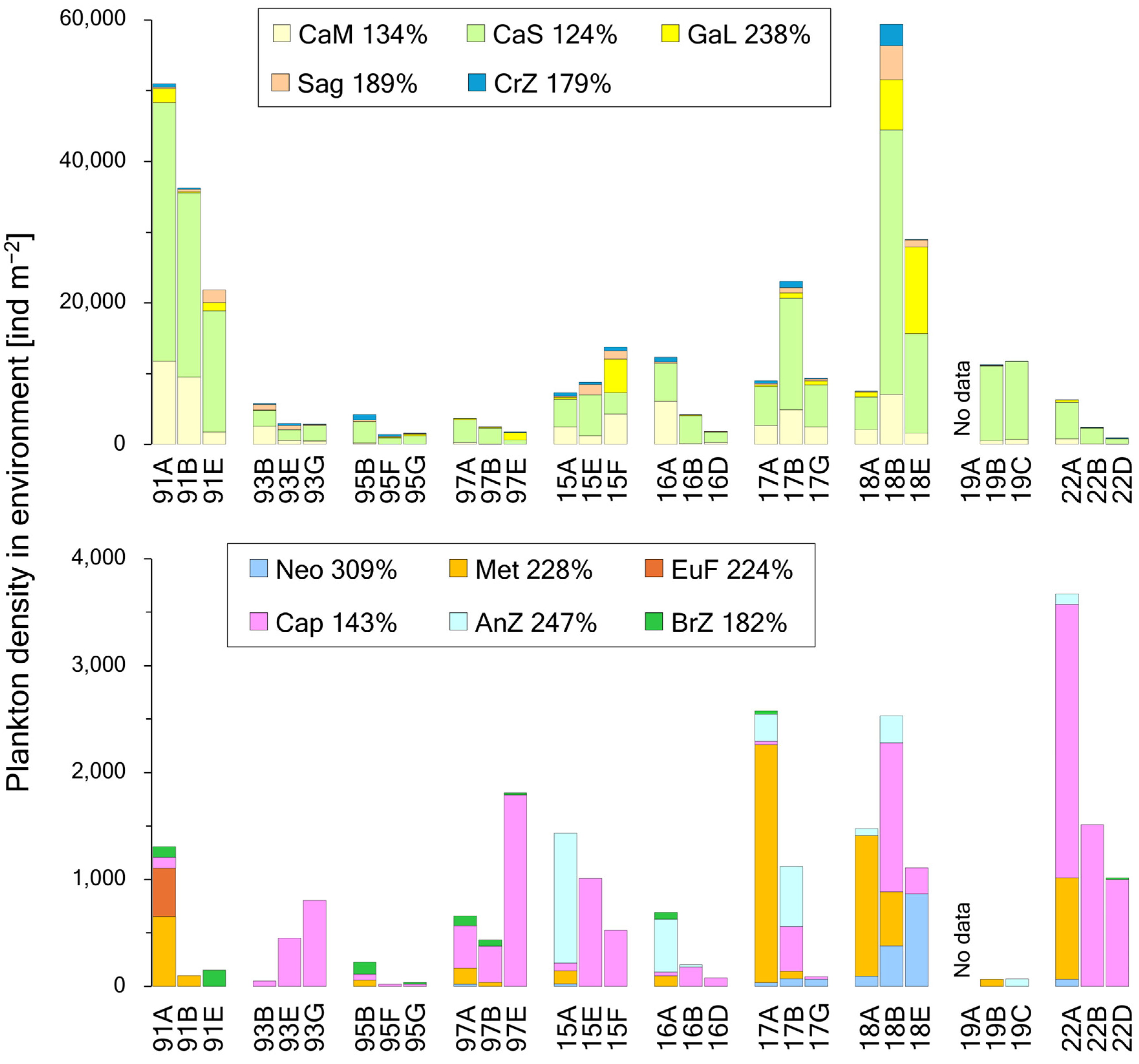
Zooplankton samples were subsampled using a plankton splitter (Available online: http://hdl.handle.net/2115/21829, accessed on 14 March 2026) [58], and >300 individuals were identified and counted under a stereomicroscope. For 11 taxa found among the prey items of Pacific cod juveniles (Table 3), densities (ind m⁻²) were estimated based on the filtered-water volume, which was calculated from flowmeter readings and towing length. Spatial variability in these densities among stations was assessed using the coefficient of variation (CV% = standard deviation × 100/mean). Differences in densities among regions (M, W, and E) were tested using the Kruskal–Wallis test with Steel–Dwass post hoc comparisons. Other prey items were not sufficiently sampled for analysis.

3. Results

3.1. Diet Composition in Pacific Cod Juveniles

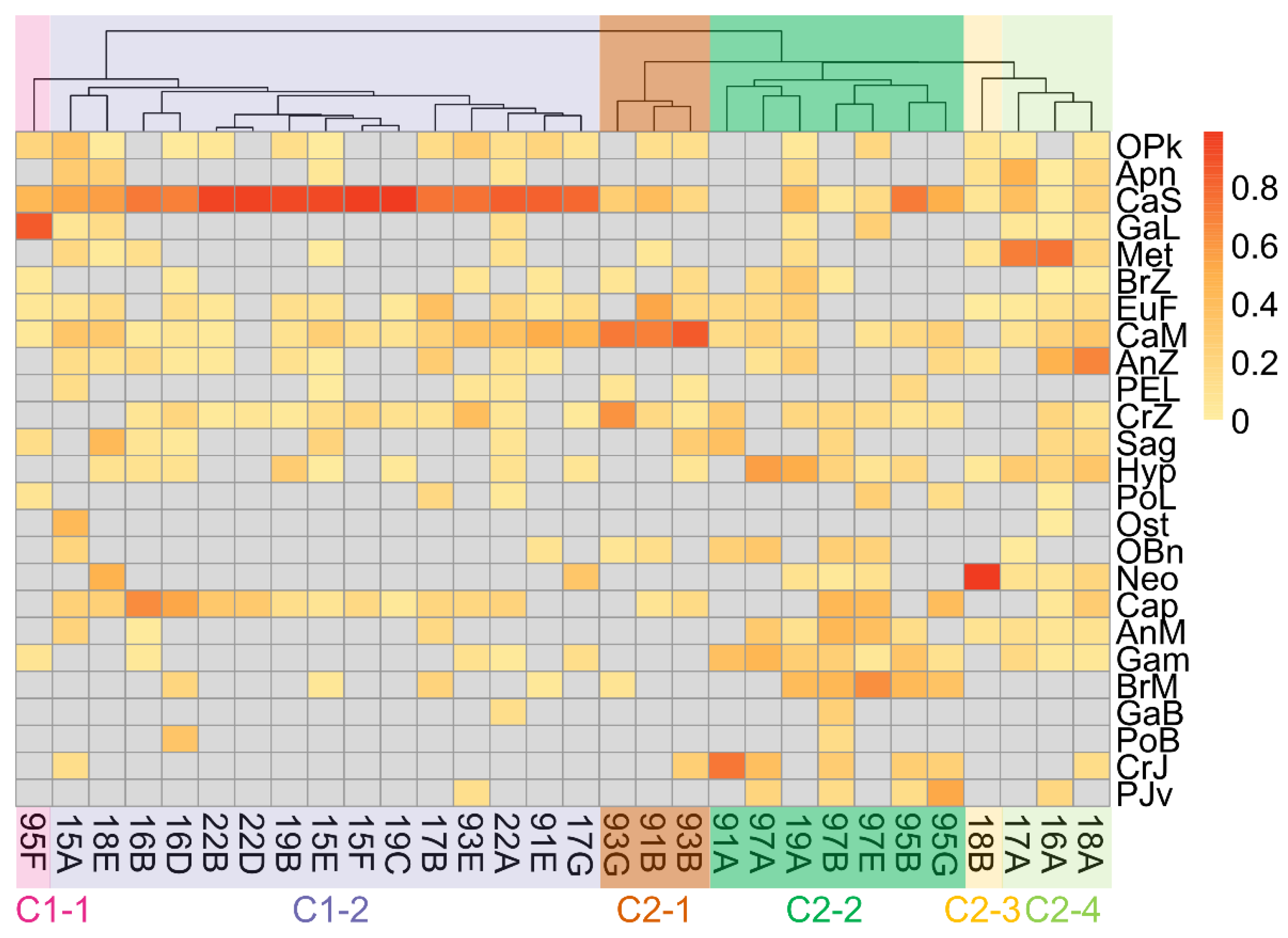
For the SCIi values in the stomach contents of Pacific cod juveniles collected at 30 stations at depths of 30–91 m (Table 2 and Table 4), the SSI [46] was highest (0.068) when the number of clusters k was 2 (Figure S1). The silhouette coefficients [47] were highest (0.236) at k = 6, with similar values for k = 4–7 (0.231–0.234). Accordingly, the stations were divided into two clusters and six subclusters (Figure 2). Subcluster 1-1 (C1-1) comprised station 95F in the innermost part of E (1995), where Gastropoda larvae (GaL) had the highest SCIi (10.86), followed by CaS (2.92; Table 2, Figure 2). C1-2 comprised 15 stations where CaS had the highest SCIi, with CaM or the planktonic ghost shrimp C. acanthogaster (Cap) ranking second. Thus, Cluster 1 (C1) comprised stations in which prey items with low Mpwp values represented the highest proportion (Table 3). The remaining 14 stations formed Cluster 2 (C2), where the prey item with the highest SCIi varied among stations. C2-1 comprised three stations in W and E (1991 and 1993) where CaM (C. pacificus and M. tenuicornis) had the highest SCIi. C2-2 was characterized by high SCIi of relatively large-sized prey (Table 2), including Pisces juveniles (PJv), Caridea juveniles (CrJ), Brachyura (crab) megalopae (BrM), benthic Gammarida (Gam), Anomura megalopae (AnM), and Hyperiidea (Hyp). C2-3 comprised only station 18B in W (2018), where cod juveniles fed on Neo, specifically on female copepodite stages 4 (19%) and 5 (81%). Neo was detected at two of the 16 C1 stations and at seven of the 14 C2 stations. C2-4 comprised three stations in M (16A, 17A, and 18A), where Anomura zoeae (AnZ) and Met had high SCIi values.

At k = 7, C2-2 split into two subclusters: (91A, 97A, and 19A) and (97B, 97E, 95B, and 95G). At k = 5, C1-1 and C1-2 formed a single cluster (i.e., C1). At k = 4, C2-3 and C2-4 merged into one subcluster.

3.2. Differences in Median SCI, Kn, and Tmp Values Between Subclusters and Areas

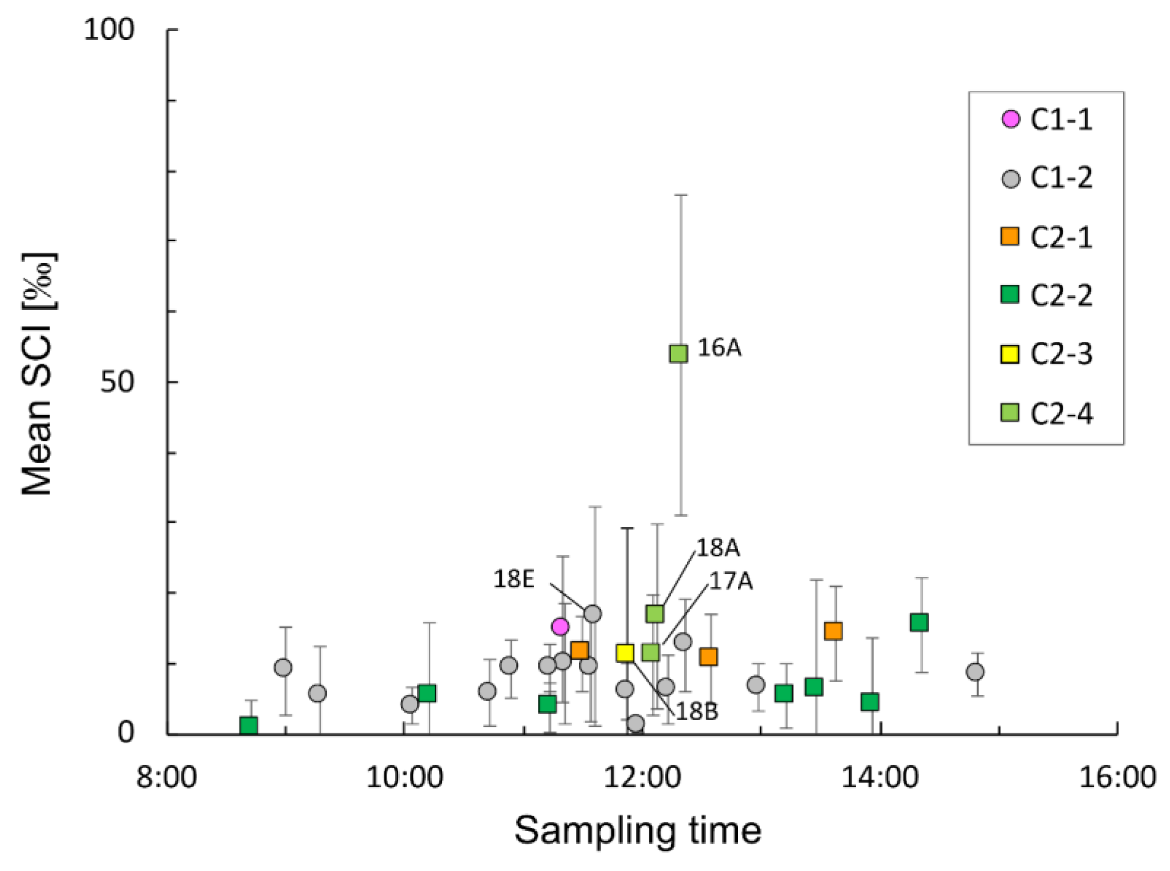
Although many fish species exhibit diel feeding rhythms and adult Pacific cod feed actively between 06:00 and 12:00 [59], no significant correlation was detected between the sampling time and feeding intensity in cod juveniles in the Mutsu Bay (Spearman’s r_s = 0.20, p = 0.15; Figure 3). At station 16A in C2-4, sampled at 12:20, juveniles showed an exceptionally high SCI (53.8‰), with high SCIi for Met (29.8‰) and AnZ (12.3‰) (Table 4; Figure 2). Stations 18A (sampled at 12:08) and 18E (sampled at 11:36) had the second- and third-highest SCI values (16.7‰ and 16.6‰, respectively). At 18A in C2-4, AnZ had high SCIi (7.7‰), whereas at 18E in C1-2, juveniles fed relatively frequently on CaS (5.3‰), Neo (3.8‰), and an arrowworm Parasagitta elegans (Sag; 2.9‰).

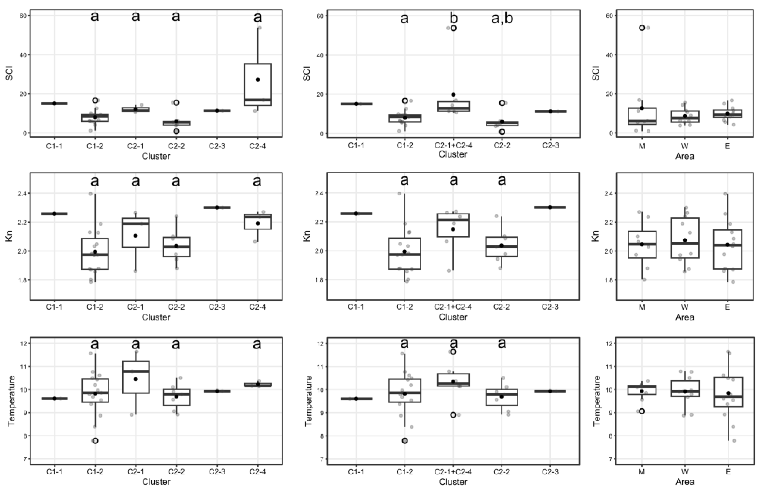
The median SCI differed insignificantly between the C1 and C2 (Mann–Whittney U test: p = 0.56), and no pairwise differences were detected among four subclusters with n ≥ 3 (C1-2: 8.4, C2-1: 11.4, C2-2: 5.3, and C2-4: 16.7; Steel–Dwass test: all p > 0.10; Figure 4). Because C2-1 and C2-4 both showed relatively high SCIi for medium-sized plankton, they were combined (C2-1 + C2-4). A significant difference was then detected between C1-2 (8.4) and C2-1 + C2-4 (12.9; Steel–Dwass test: p = 0.011), whereas not between C1-2 and C2-2 (p = 0.078) and between C2-1 + C2-4 and C2-2 (p = 0.16; Figure 4). Median SCI differed insignificantly among the three areas (M, W, and E; Kruskal–Wallis test: p = 0.59).

No significant differences in Kn and Tmp were found among subclusters (Steel–Dwass test: Kn p > 0.17; Tmp p > 0.52; Figure 4) or among the three areas (Kruskal–Wallis test: p = 0.90 and 0.91).

3.3. Ordination of Diet Composition

Across all five ordination models, VIF for Kn, Tmp, TL, and Dist_YJ was 1.11–1.35, well below the commonly cited threshold for considerable collinearity (VIF ≥ 2.5) [60]. The mean TL decreased with sampling year (r = −0.82, p < 0.001; Figure S2). Therefore, sampling year was excluded as an explanatory variable.

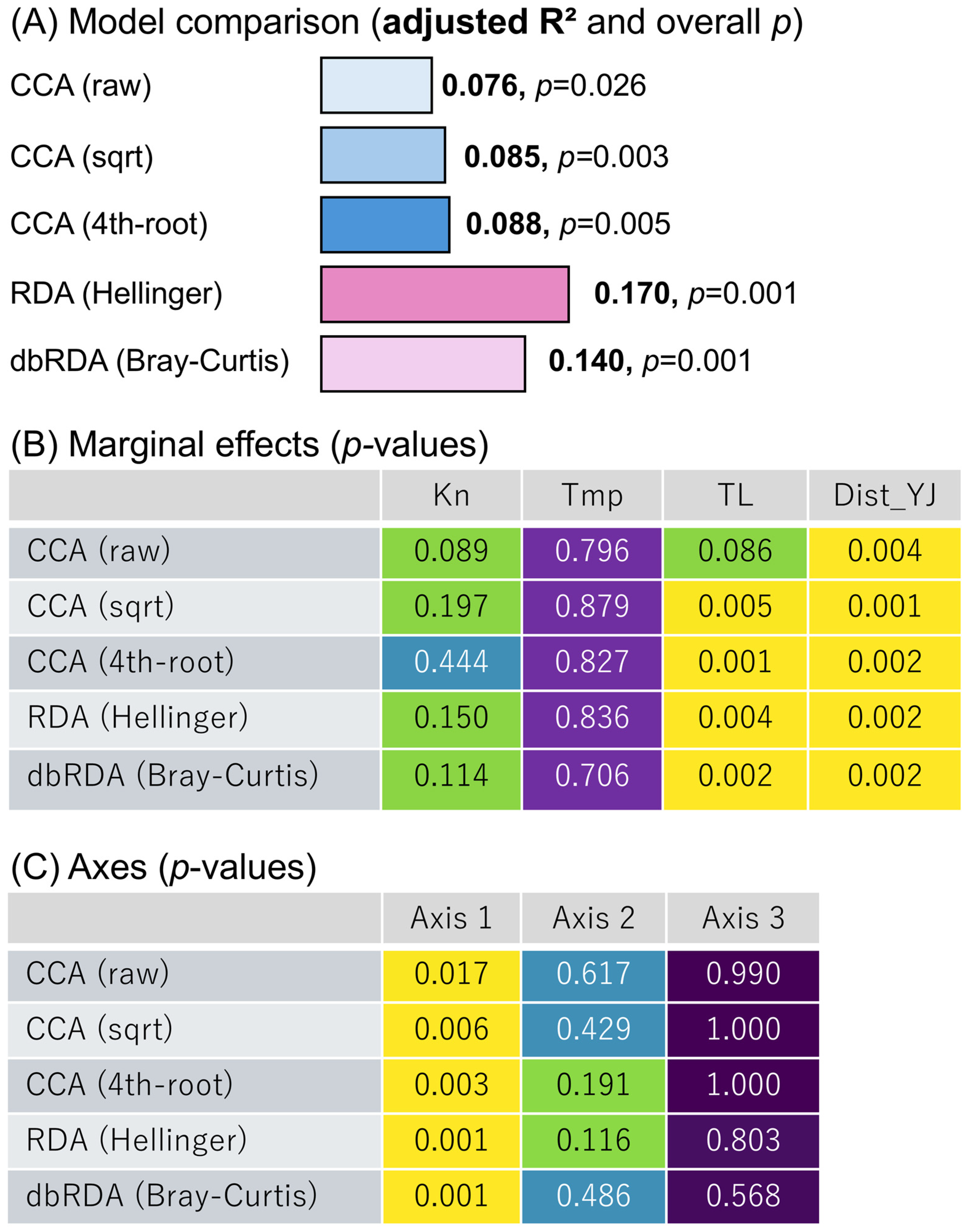
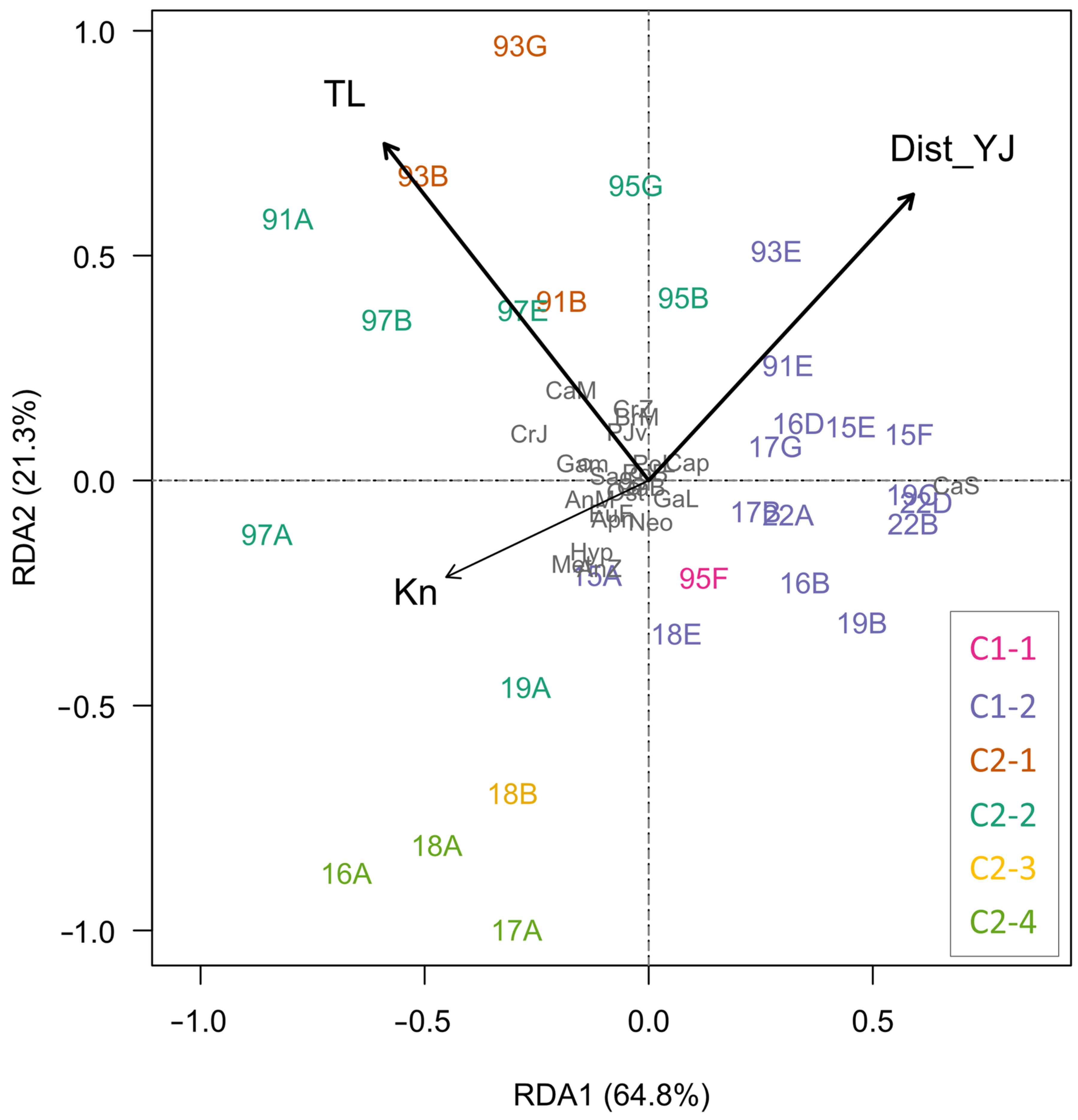
The length of the first DCA axis was 3.95 standard deviation (SD) units. Following Lepš and Šmilauer [50], both RDA (<3 SD) and CCA (>4 SD) approaches were evaluated. The Hellinger-transformed RDA showed the highest adjusted R² (0.170) and was significant overall (p = 0.001; Figure 5). In marginal tests, TL (p = 0.004) and Dist_YJ (p = 0.002) were significant, whereas Tmp and Kn were not (p = 0.84 and p = 0.15, respectively). Axis 1 was significant (p = 0.001), but Axis 2 was not (p = 0.12). TL, Kn, and Dist_YJ were correlated with Axis 1 (r = −0.50, −0.38, and +0.50; p = 0.005, 0.039, and 0.005, respectively; Figure 6), indicating that sampling stations with lower Axis 1 scores had larger TL and higher Kn and were located closer to the bay mouth. Prey distributions followed a similar pattern: smaller-sized CaS and GaL plotted positively on Axis 1, whereas the relatively larger-sized CrJ, CaM, Met, Gam, AnM, AnZ, and Sag plotted negatively.

3.4. Factors Affecting the Relative Condition Factor (Kn) and Their Effect Sizes

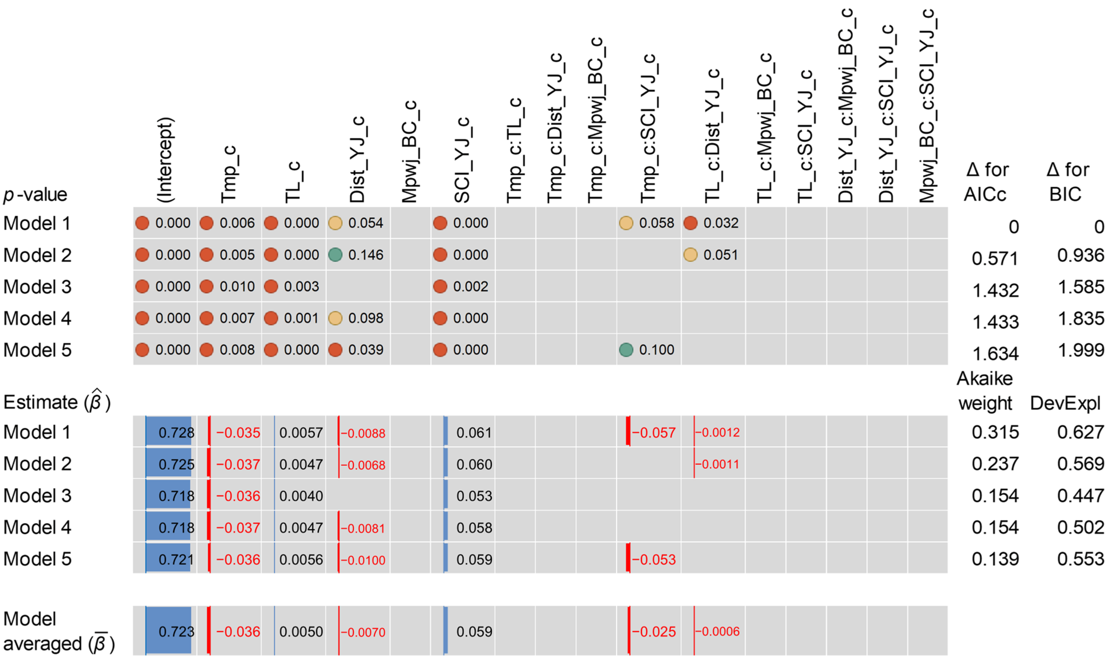
The best GLM explaining temporal changes in Kn across three stations over 10 years was Model 1 (ΔAICc = 0), which was also selected as the minimum model by BIC. In Model 1, the interaction between TL_c and Dist_YJ_c (TL_c:Dist_YJ_c) was negative and significant ($\widehat{\beta }$ = −0.0012, p = 0.032), while interaction term Tmp_c:SCI_YJ_c was negative and marginally significant ($\widehat{\beta }$= −0.057, p = 0.058; Figure 7). Four main-effect terms included Tmp_c, TL_c, Dist_YJ_c, and SCI_YJ_c and were significant or marginally significant ($\widehat{\beta }$ = −0.035–0.061, p = 0.000–0.054). Mpwj_BC_c was not selected for the final model; however, TL and Mpwj_BC were significantly positively correlated (r = 0.60, p = 0.0004; Figure S2).

Among the candidate models, four (Models 2–5) had ΔAICc ≤2 and were subsets of Model 1. Two of these models included one negative interaction term each (TL_c:Dist_YJ_c: $\widehat{\beta }$ = −0.0011 p = 0.051; Tmp_c:SCI_YJ_c: $\widehat{\beta }$ = −0.053 p = 0.10). The main effects were consistent across Models 1–5: Tmp_c had negative effects ($\widehat{\beta }$ = −0.037–−0.035, p = 0.005–0.010); TL_c had positive effects ($\widehat{\beta }$ = 0.0040–0.0057, p = 0.000–0.003), SCI_YJ_c had positive effects ($\widehat{\beta }$ = 0.053–0.061, p = 0.000–0.002), and Dist_YJ_c had negative effects ($\widehat{\beta }$ = −0.010–−0.007, p = 0.039–0.146). Among the top five models, improvement over the intercept-only (null) model, as measured by deviance explained (DevExpl), ranged from 44.7% to 62.7%.

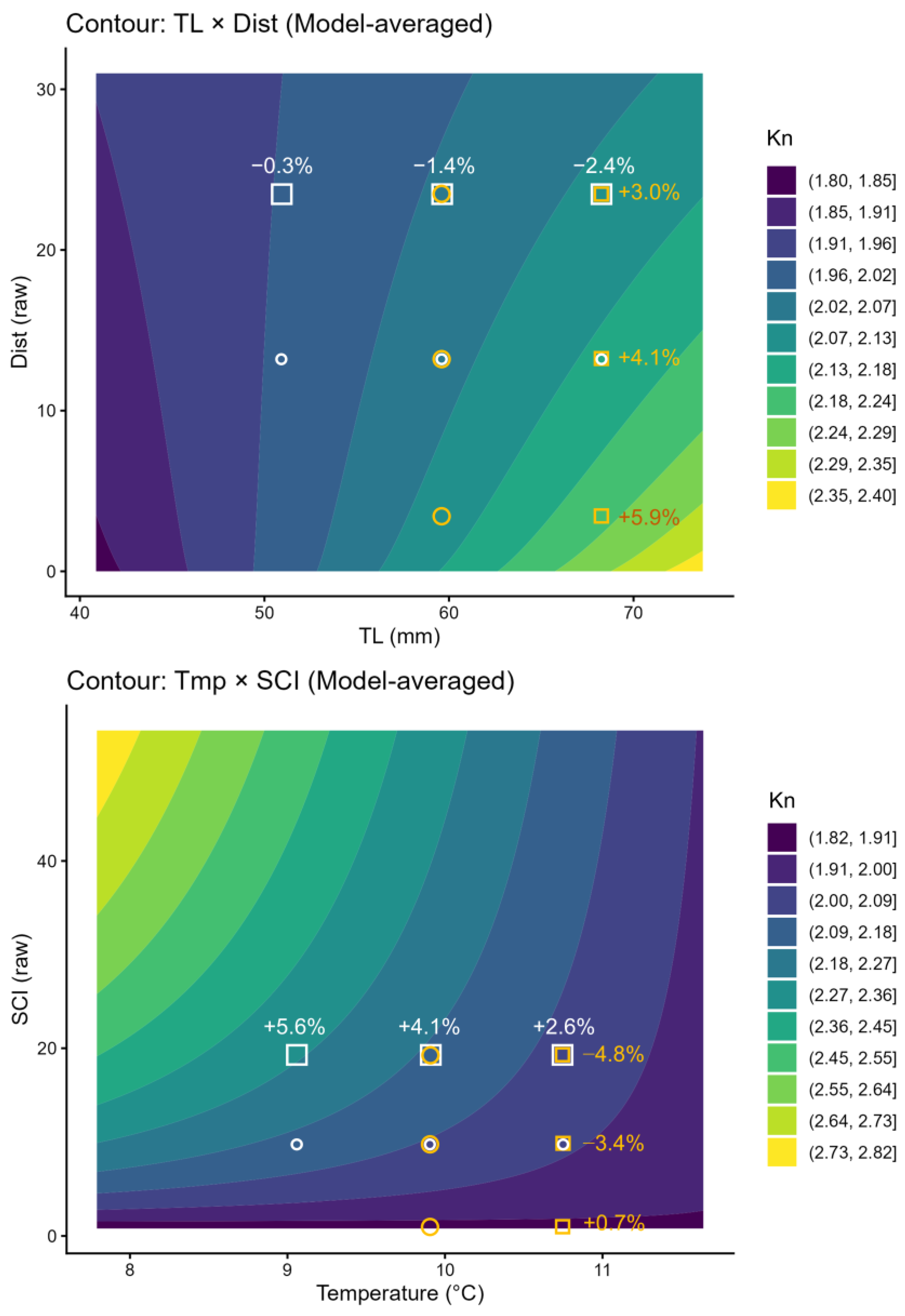
Model averaging across Models 1–5, based on Akaike weights, indicated weak antagonistic interactions between TL and Dist ($\widehat{\beta }$ = −0.0006) and between Tmp and SCI ($\widehat{\beta }$ = −0.025; Figure 7). The positive effect of TL on Kn decreased with increasing distance from station 15A in M, while the negative effect of distance strengthened for larger-sized juveniles (Figure 8). Higher SCI amplified the negative effect of Tmp on Kn, and the positive effect of SCI weakened under warmer conditions. For the main effects under mean + one-unit conditions, TL (59.5 + 8.68 mm: +4.1%) and SCI (10.15 + 9.30‰: +4.1%) had stronger positive effects on Kn than the negative effects of Dist (13.33 + 9.99 mile: −1.4%) and Tmp (9.89 °C + 0.84 °C: −3.4%; Figure 8).

3.5. Geographical Differences of Zooplankton Density in Plankton-Net Samples

The densities of 11 major planktonic prey items at 29 stations (excluding 19A, where data were missing) varied significantly by sampling year and location (Figure 9). Among the stations, the CV% was highest for Neo (309%) and lowest for CaS, CaM, and Cap (124%, 134%, and 143%, respectively). Among the sampling areas (M, W, and E), three plankton groups commonly consumed by cod juveniles (Met, AnZ, and EuF) showed significant regional differences (Kruskal–Wallis test: p < 0.001, 0.049, and <0.001, respectively). In all three cases, median densities were highest in M, with no individuals collected in E. Although Neo showed no significant difference in median density across the three areas (Kruskal–Wallis test: p = 0.28), its occurrence frequency differed significantly among regions (G-test: G_adj. = 6.18, p = 0.046). Neo occurred in five of seven stations in M, but only in two of 10 stations in W and two of 12 stations in E, indicating higher occurrence in M. To evaluate the potential effects of net mouth diameter on density estimates, we compared the total plankton density between the 45 and 80 cm nets. The median total density was 4153 ind m⁻² for the 45 cm net and 10,817 ind m⁻² for the 80 cm net, with no statistically significant difference between the nets (Mann–Whitney U test: p = 0.11).

Figure 9. Densities (ind m⁻²) and coefficients of variation (CV%) of the major planktonic taxa consumed by juvenile Pacific cod, based on vertical tows using two plankton nets with different mouth diameters (mesh aperture: 0.335 mm; 45 cm diameter in 1991–1997 and 80 cm diameter in 2015–2022). The 2019 data for station A are missing. The six taxa with maximum density < 3000 ind m⁻² (Neo: N. plumchrus, Met: M. pacifica, EuF: E. pacifica, Cap: C. acanthogaster, ArZ: Anomura zoea, and BrZ: Brachyura zoea) are shown in the lower panel, whereas the five taxa with maximum density of ≥3000 ind m⁻² (CaM, CaS, GaL: Gastropoda larva, Sag: P. elegans, and CrZ: Caridea zoea) are shown in the upper panel.

Figure 9. Densities (ind m⁻²) and coefficients of variation (CV%) of the major planktonic taxa consumed by juvenile Pacific cod, based on vertical tows using two plankton nets with different mouth diameters (mesh aperture: 0.335 mm; 45 cm diameter in 1991–1997 and 80 cm diameter in 2015–2022). The 2019 data for station A are missing. The six taxa with maximum density < 3000 ind m⁻² (Neo: N. plumchrus, Met: M. pacifica, EuF: E. pacifica, Cap: C. acanthogaster, ArZ: Anomura zoea, and BrZ: Brachyura zoea) are shown in the lower panel, whereas the five taxa with maximum density of ≥3000 ind m⁻² (CaM, CaS, GaL: Gastropoda larva, Sag: P. elegans, and CrZ: Caridea zoea) are shown in the upper panel.

4. Discussion

4.1. Diet Patterns and Spatial Structure

Most diet research on early survival in marine fishes has focused on whether larvae successfully initiate feeding (e.g., [61,62]), a stage when larvae are morphologically underdeveloped and weak swimmers, and feeding success is still regarded as a stage in which recruitment variability is strongly influenced. In contrast, many demersal fishes are pelagic during the larval stage and settle to the seabed from the late larval to early juvenile stages, accompanied by dietary shifts [23]. However, relationships between diet and nutritional condition immediately after settlement remain poorly studied [63]. In the present study, we examined settled age-0 Pacific cod juveniles in Mutsu Bay. Using 10 years of data from the three stations with the highest juvenile densities per year, we quantified the SCIi and evaluated its relationships with juvenile attributes and environmental factors. We further modeled Kn using juvenile attributes, SCI, and environmental factors, thereby assessing the relationship between feeding level and nutritional condition.

During the settlement period in Mutsu Bay, juveniles primarily consumed CaS (<0.1 mg ind⁻¹ in Mpwp) at 16 of the 30 stations; CaM (0.1–1.0 mg ind⁻¹), Met, and AnZ at six stations; N. plumchrus (Neo; 1.24 mg ind⁻¹) at one station; and various relatively larger prey, including benthos (>2 mg ind⁻¹), at seven stations (Figure 2). Station-specific diets were broadly classified into C1 (a high proportion of relatively small-sized plankton) and C2 (characterized by mixtures including relatively larger prey). RDA ordination similarly separated C1 (positive RDA1) and C2 (negative RDA1), indicating that RDA1 reflects prey size, predator TL, and distance from sampling station to M 15A (Figure 6). Because TL correlated positively with Mpwj_BC (r = 0.60; Figure S2), RDA1 likely also represented an ontogenetic index of dietary shifting. Medium-sized plankton (Met, AnZ, and Euphausiacea furciliae (EuF)) and large-sized Calanoida (N. plumchrus; Neo), frequently consumed in C2-1, C2-3, and C2-4, had higher densities in plankton-net samples from M and W (Figure 9), suggesting that prey availability partly influenced juvenile diets.

Although six subclusters were identified (Figure S1), silhouette coefficients for k = 4–7 were similar (0.231–0.234), indicating weak structure [47]. In subclusters C1-1, C1-2, and C2-1, the prey item with the highest SCIi was consistent across stations, whereas C2-4 showed interchange between top-ranked and second-ranked prey by SCIi, and C2-2 exhibited higher variability in dominant prey. Thus, C2-2 and C2-4 were not clearly distinct, and the small differences in silhouette coefficients within C2 suggest that SCIi composition varied along a continuum. Nevertheless, C2-2 consistently included large prey items with high Mpwp (Table 3) and were distributed broadly on the negative side of RDA1 (Figure 6). Because five of the seven C2-2 stations were located in M or W, larger prey, including benthos (>2 mg ind⁻¹), may have been more available or more readily exploited in these areas. Although environmental abundance data for these large prey were lacking, Gam specimens collected by grab sampling are reported to be common on the seafloor in M [22]. In the Chukchi Sea, age-0 Pacific cod collected using a demersal trawl fed on a wide variety of benthic and near-benthic taxa, including polychaetes, amphipods, nematodes, and epibenthic copepods, demonstrating high dietary diversity comparable to that found in Mutsu Bay in this study [28]. Cooper et al. [28] further discussed that such dietary differences primarily reflect habitat selection. In this study, juveniles that consumed relatively large prey fed on a wide variety of prey taxa, showing a similar pattern of opportunistic feeding on prey encountered in their habitat.

4.2. Feeding Limitation and Condition Dynamics

Mutsu Bay has been considered a nursery habitat for Pacific cod because adults migrate into the bay from December to February to spawn, and settled juveniles occur at high abundance from late May to June [22]. However, our results indicate that, across all years examined, settled juveniles rarely consumed sufficiently large amounts of prey, suggesting that the post-settlement period may represent a stage of increased risk for reduced survival. Juveniles showed an extremely high mean SCI at only one station (53.8‰ at 16A; Table 2 and Table 4; Figure 3), indicating that comparable feeding intensity might be achievable at other stations under favorable conditions. In reality, however, SCI values at the other 29 stations remained low (≤16.7‰). In a previous study from April 1990 in Mutsu Bay, pelagic larvae and small juveniles (20.9–42.7 mm TL) showed an SCI value (Scw × 100/Bwt, including digested material) of 29‰ ± 13.4‰ [23], which exceeds values observed at the 29 stations in our study, excluding station 16A (53.8‰), after late May. Moreover, SCI did not increase during daytime for settled juveniles after late May (Figure 3). These patterns suggest that prey density was insufficient and/or that higher water temperatures caused gastric evacuation and digestion rates to exceed prey intake more readily [64,65,66].

At the six stations in C2-1 and C2-4, juveniles consumed medium-sized plankton, and median SCI tended to be higher, yet median Kn and Tmp did not differ from those of other subclusters (Figure 4). This discrepancy likely reflects the fact that Kn is influenced by multiple factors beyond SCI, including Tmp, juvenile body size, and the probability of encountering relatively large prey. In the GLM-based comparisons using ±1-unit changes from mean values, Kn increased with juvenile body size (TL: +4.1%) and feeding intensity (SCI: +4.1%), whereas water temperature showed a somewhat weaker negative effect (Tmp: −3.4%), and distance from M showed a weak negative effect (Dist: −1.4%; Figure 8). A maximum effect of +4.1% is not large in absolute terms; however, Mutsu Bay during this period represents a high-temperature environment close to the upper thermal limit for this species. Under such conditions, even small individual differences in body condition may have a substantial effect on survival. Additionally, both estimated interaction terms (TL_c:Dist_YJ_c and Tmp_c:SCI_YJ_c) were negative (Figure 7), indicating antagonistic (offsetting) patterns. Specifically, the positive effect of increasing TL on Kn was reduced in the inner bay where Dist was larger, and the positive effect of SCI reduced as Tmp increased. Because Met, AnZ, and EuF—among the medium-sized prey—were scarcely distributed in the inner bay (Figure 9), feeding opportunities were likely more limited farther into the bay. Pacific cod juveniles rarely occur at stations warmer than 12 °C, which is considered an upper thermal habitat limit [22]. In this study, Kn reduced as Tmp approached this upper limit, even when prey consumption increased (Figure 8), suggesting that high metabolic rates under warm condition hinder energy accumulation. Therefore, earlier movement toward M is likely beneficial for juvenile Pacific cod in the Mutsu Bay, particularly for larger-sized juveniles. Occupying cooler stations may also help juveniles maintain higher Kn and improve survival. The bay mouth provides easier access to offshore areas with greater depths and expected lower water temperatures; thus, this area was considered advantageous for survival. Kd tended to increase with TL in the present study (Figure 8), whereas Farley et al. [25] demonstrated that juvenile body size is not always a reliable indicator of energetic condition, indicating that nutritional condition is more strongly influenced by prey type and quality than by body length alone.

Among the taxa examined, N. plumchrus (Neo) showed the highest among-station variability in density (CV% = 309%), suggesting a patchy distribution and that encounters are infrequent. In Mutsu Bay, the inflow of the TgWC varies substantially depending on the water-mass density between bay water and inflowing TgWC, and copepod community composition can change markedly across years [18]. N. plumchrus, like M. pacifica (Met), primarily inhabits offshore waters [67,68] and is likely transported into the by the TgWC, expanding its distribution from winter to spring. Thus, interannual variation in TgWC inflow may underlie the high variability in zooplankton abundance. However, N. plumchrus was detected in juvenile stomachs at only nine of the 30 stations, limiting the assessment of its effects on SCI or Kn.

4.3. Limitations of This Study and Future Perspectives

Median SCI did not differ among most clusters; a difference was detected only when stations dominated by medium-sized prey (C2-1 and C2-4 combined; 12.9) were compared with C1-2 (8.4). In C1-2, juveniles primarily consumed small CaS. Previous studies suggest that, given the costs of feeding, successfully consuming prey of moderate and appropriate size relative to predator body size may be most important for net energy gain and energy storage, even at similar feeding levels [69,70,71]. Pepin [72] further distinguished between “high-feeding-ability” and “low-feeding-ability” individuals within narrow size classes across 11 larval fish species, showing that strong foragers preferentially consumed smaller prey and exhibited higher responsiveness and attack probability following encounters. Therefore, future studies should include rearing experiments and behavioral observations of juvenile Pacific cod to quantify prey selection, handling time, oxygen consumption, and individual physiological state using bioenergetic models to identify traits associated with higher survival. Additionally, relatively larger-sized prey items consumed by juveniles in C2-2 with Mpwp >2.0 mg ind⁻¹, including Anomura megalopae (AnM), Brachyura megalopae, Caridea juveniles, and Pisces juveniles (PJv) (Figure 2), were not adequately sampled by the plankton nets, preventing accurate estimation of their environmental abundances. Clarifying the abundances of these relatively larger prey organisms should therefore be an important objective for future studies.

5. Conclusions

Our long-term analysis revealed that feeding conditions during settlement are associated with the nutritional condition of demersal juvenile fish. In juvenile Pacific cod in Mutsu Bay, stomach-content weight (SCI) reached 53.8‰ of body weight at one station near the bay mouth and 16.7‰ at the other 29 stations; no clear diel feeding periodicity was detected. These results indicate that many juveniles did not accumulate prey in the stomach during the day. Kn increased with juvenile TL and SCI and appeared to be higher in cooler, bay-mouth areas, but did not consistently increase in juveniles dominated by any single prey taxon. After settlement, juveniles likely face demands to rapidly shift their feeding strategy to match habitat conditions; however, juveniles may not always encounter prey of an appropriate size that contributes to growth. Together, these patterns indicate that spatial variation in prey encounter opportunities (indexed by distance from the bay mouth) and elevated temperatures that increase metabolic demand may limit net energy accumulation, with potential implications for recruitment dynamics and nursery-habitat evaluation. Continued warming may shorten the period during which juveniles of this cold-water species can remain within this nursery habitat and may weaken its nursery function.

References

1. Hjort, J. Fluctuations in the great fisheries of northern Europe viewed in the light of the biological research. Rapp. p.v. Reun. Cons. Int. Explor. Mer. 1914, 20, 1–228. [Google Scholar]
2. Cushing, D.H.; Dickson, R.R. The biological response in the sea to climatic change. Adv. Mar. Biol. 1976, 14, 1–112. [Google Scholar]
3. Hunter, J.R. Feeding ecology and predation of marine fish larvae. In Marine Fish Larvae; Lasker, R., Ed.; Washington Sea Grant Program: Washington, DC, USA, 1981; pp. 33–77. [Google Scholar]
4. van der Veer, H.W.; Bergman, M.J.N. Predation by crustaceans on a newly settled 0-group plaice Pleuronectes platessa population in the western Wadden Sea. Mar. Ecol. Prog. Ser. 1987, 35, 201–215. [Google Scholar] [CrossRef]
5. Houde, E.D. Fish early life dynamics and recruitment variability. Am. Fish. Soc. Symp. 1987, 2, 17–29. [Google Scholar]
6. Anderson, J.T. A review of size dependent survival during pre-recruit stages of fishes in relation to recruitment. J. Northw. Atl. Fish. Sci. 1988, 8, 55–66. [Google Scholar] [CrossRef]
7. Litvak, M.K.; Leggett, W.C. Age and size-selective predation on larval fishes: The bigger-is-better hypothesis revisited. Mar. Ecol. Prog. Ser. 1992, 81, 13–24. [Google Scholar] [CrossRef]
8. Pepin, P.; Shears, T.H.; de Lafontaine, Y. Significance of body size to the interaction between a larval size (Mallotus villosus) and a vertebrate predator (Gasterosteus aculeatus). Mar. Ecol. Prog. Ser. 1992, 81, 1–12. [Google Scholar] [CrossRef]
9. Watanabe, Y.; Zenitani, H.; Kimura, R. Population decline of the Japanese sardine Sardinops melanostictus owing to recruitment failures. Can. J. Fish. Aquat. Sci. 1995, 52, 1609–1616. [Google Scholar] [CrossRef]
10. Campana, S.E. Year-class strength and growth rate in young Atlantic cod Gadus morhua. Mar. Ecol. Prog. Ser. 1996, 135, 21–26. [Google Scholar] [CrossRef]
11. Takasuka, A.; Aoki, I.; Mitani, I. Evidence of growth-selective predation on larval Japanese anchovy Engraulis japonicus in Sagami Bay. Mar. Ecol. Prog. Ser. 2003, 252, 223–238. [Google Scholar] [CrossRef]
12. Joh, M.; Nakaya, M.; Yoshida, N.; Takatsu, T. Interannual growth differences and growth-selective survival in larvae and juveniles of marbled sole Pseudopleuronectes yokohamae. Mar. Ecol. Prog. Ser. 2013, 494, 267–279. [Google Scholar] [CrossRef][Green Version]
13. Chambers, R.C.; Waiwood, K.G. Maternal and seasonal differences in egg sizes and spawning characteristics of captive Atlantic cod, Gadus morhua. Can. J. Fish. Aquat. Sci. 1996, 53, 1986–2003. [Google Scholar] [CrossRef]
14. Kjesbu, O.S.; Solemdal, P.; Bratland, P.; Fonn, M. Variation in annual egg production in individual captive Atlantic cod (Gadus morhua). Can. J. Fish. Aquat. Sci. 1996, 53, 610–620. [Google Scholar] [CrossRef]
15. Higashitani, T.; Takatsu, T.; Nakaya, M.; Joh, M.; Takahashi, T. Maternal effects and larval survival of marbled sole Pseudopleuronectes yokohamae. J. Sea Res. 2007, 58, 78–89. [Google Scholar] [CrossRef]
16. Kajiwara, K.; Nakaya, M.; Suzuki, K.; Kano, Y.; Takatsu, T. Effect of egg size on the growth rate and survival of wild walleye pollock Gadus chalcogrammus larvae. Fish. Oceanogr. 2022, 31, 238–254. [Google Scholar] [CrossRef]
17. Ketchen, K.S. Observations on the ecology of the Pacific cod (Gadus macrocephalus) in Canadian waters. J. Fish. Res. Board. Can. 1961, 18, 513–558. [Google Scholar] [CrossRef]
18. Takatsu, T.; Nakatani, T.; Miyamoto, T.; Kooka, K.; Takahashi, T. Spatial distribution and feeding habits of Pacific cod (Gadus macrocephalus) larvae in Mutsu Bay, Japan. Fish. Oceanogr. 2002, 11, 90–101. [Google Scholar] [CrossRef]
19. Fukuda, S.; Yokoyama, K.; Hayakawa, Y.; Nakanishi, H. On tagging experiments of adult Pacific cod in the entrance of Mutsu Bay, Aomori Prefecture. Saibai Gyogyo Gijutsu Kaihatsu Kenkyu 1985, 14, 71–77. (In Japanese) [Google Scholar]
20. Sakurai, Y.; Takahashi, T. (Hokkaido University, Hakodate, Hokkaido, Japan). 1991; Unpublished work.
21. Ohtani, K.; Terao, T. Oceanographic structure of the Mutsu Bay. Bull. Fac. Fish. Hokkaido Univ. 1974, 24, 100–131. (In Japanese) [Google Scholar]
22. Takatsu, T.; Yoshida, Y.; Kooka, K.; Sugimoto, K.; Takahashi, T. Spatial and temporal distribution of Pacific cod Gadus macrocephalus juveniles in Mutsu Bay, Japan. Bull. Jpn. Soc. Fish. Oceanogr. 2001, 65, 6–14. [Google Scholar]
23. Takatsu, T.; Nakatani, T.; Mutoh, T.; Takahashi, T. Feeding habits of Pacific cod larvae and juveniles in Mutsu Bay, Japan. Fish. Sci. 1995, 61, 415–422. [Google Scholar] [CrossRef]
24. Takatsu, T. Early Life History of Gadus macrocephalus in Mutsu Bay. Ph.D. Dissertation, Hokkaido University, Hakodate, Japan, 25 December 1998. Available online: https://hdl.handle.net/2115/32724 (accessed on 14 March 2026). (In Japanese) [CrossRef]
25. Farley, E.V., Jr.; Heintz, R.A.; Andrews, A.G.; Hurst, T.P. Size, diet, and condition of age-0 Pacific cod (Gadus macrocephalus) during warm and cool climate states in the eastern Bering Sea. Deep Sea Res. Part II Top. Stud. Oceanogr. 2016, 134, 247–254. [Google Scholar] [CrossRef]
26. Abookire, A.A.; Duffy-Anderson, J.T.; Jump, C.M. Habitat associations and diet of young-of-the-year Pacific cod (Gadus macrocephalus) near Kodiak, Alaska. Mar. Biol. 2007, 150, 713–726. [Google Scholar] [CrossRef]
27. Strasburger, W.W.; Hillgruber, N.; Pinchuk, A.I.; Mueter, F.J. Feeding ecology of age-0 walleye pollock (Gadus chalcogrammus) and Pacific cod (Gadus macrocephalus) in the southeastern Bering Sea. Deep Sea Res. Part II Top. Stud. Oceanogr. 2014, 109, 172–180. [Google Scholar] [CrossRef]
28. Cooper, D.W.; Cieciel, K.; Copeman, L.; Emelin, P.O.; Logerwell, E.; Ferm, N.; Jesse, L.; Levine, R.; Axler, K.; Woodgate, R.A.; et al. Pacific cod or tikhookeanskaya treska (Gadus macrocephalus) in the Chukchi Sea during recent warm years: Distribution by life stage and age-0 diet and condition. Deep Sea Res. Part II Top. Stud. Oceanogr. 2023, 208, 105241. [Google Scholar] [CrossRef]
29. Thalmann, H.L.; Laurel, B.J.; Almeida, L.Z.; Osborne, K.E.; Marshall, K.; Miller, J.A. Marine heatwaves alter the nursery function of coastal habitats for juvenile Gulf of Alaska Pacific cod. Sci. Rep. 2024, 14, 14018. [Google Scholar] [CrossRef]
30. Odamaki, M. Tides and currents. In Japan National Coastal Oceanography; Editorial Committee of the “Coastal Ocean Journal” of the Coastal Ocean Research Division of the Japan Society of Oceanography, Ed.; Tokai University Press: Tokyo, Japan, 1985; pp. 145–149. (In Japanese) [Google Scholar]
31. Maeda, T.; Nakatani, T.; Takahashi, T.; Ueno, M. Transport and migration of the walleye pollack larvae in the coastal waters. Bull. Jap. Soc. Fish. Oceanogr. 1979, 34, 81–85. (In Japanese) [Google Scholar]
32. Takatsu, T.; Suzuki, Y.; Shimizu, A.; Imura, K.; Hiraoka, Y.; Shiga, N. Feeding habits of larval stone flounder Platichthys bicoloratus in Mutsu Bay, Japan. Fish. Sci. 2007, 73, 142–155. [Google Scholar] [CrossRef]
33. Tsuda, A.; Saito, H.; Kasai, H. Life histories of Neocalanus femingeri and Neocalanus plumchrus (Calanoida: Copepoda) in the western subarctic Pacific. Mar. Biol. 1999, 135, 533–544. [Google Scholar] [CrossRef]
34. Hirai, J.; Chen, F.; Itoh, H.; Tadokoro, K.; Lemay, M.A.; Hunt, B.P.V.; Tuda, A. Molecular and morphological analyses to improve taxonomic classification of Metridia lucens/pacifica in the North Pacific. J. Plankton Res. 2022, 44, 454–463. [Google Scholar] [CrossRef]
35. Hosono, T.; Sakurai, Y. Life history of Caprella acanthogaster (Amphipoda, Crustacea), a fouling organism on fishery facilities. Aquac. Sci. 2006, 54, 107–114. [Google Scholar]
36. Le Cren, E.D. The length-weight relationship and seasonal cycle in gonad weight and condition in the perch (Perca fluviatilis). J. Anim. Ecol. 1951, 20, 201–219. [Google Scholar] [CrossRef] [PubMed]
37. R Core Team. R: A Language and Environment for Statistical Computing. R Foundation for Statistical Computing. 2025. Available online: https://www.R-project.org/ (accessed on 13 August 2025).
38. Oksanen, J.; Simpson, G.L.; Blanchet, F.G.; Kindt, R.; Legendre, P.; Minchin, P.R.; O’hara, R.B.; Solymos, P.; Stevens, M.H.H.; Szoecs, E.; et al. vegan: Community Ecology Package, R package version 2.7-3. 2026. Available online: https://cran.r-project.org/web/packages/vegan/index.html (accessed on 14 March 2026).
39. Fox, J.; Weisberg, S. An R Companion to Applied Regression; Sage Publications: Thousand Oaks, CA, USA, 2019. [Google Scholar]
40. Bartoń, K. MuMIn: Multi-Model Inference, R Package Version 1.48.11. 2025. Available online: https://CRAN.R-project.org/package=MuMIn (accessed on 1 June 2025).
41. Wickham, H. ggplot2: Elegant Graphics for Data Analysis; Springer: New York, NY, USA, 2016. [Google Scholar]
42. Kolde, R. pheatmap: Pretty Heatmaps, Version 1.0.13. 2025. Available online: https://cran.r-project.org/web/packages/pheatmap/index.html (accessed on 13 August 2025).
43. Galili, T. dendextend: An R package for visualizing, adjusting and comparing trees of hierarchical clustering. Bioinformatics 2015, 31, 3718–3720. [Google Scholar] [CrossRef]
44. Ward, J.H., Jr. Hierarchical grouping to optimize an objective function. J. Am. Stat. Assoc. 1963, 58, 236–244. [Google Scholar] [CrossRef]
45. Rao, C.R. The use and interpretation of principal component analysis in applied research. Sankhyā Indian J. Stat. Ser. A 1964, 26, 329–358. [Google Scholar]
46. Dolnicar, S.; Grabler, K.; Mazanec, J.A. A tale of three cities: Perceptual charting for analyzing destination images. In Consumer Psychology of Tourism, Hospitality and Leisure; Woodside, A.G., Crouch, G.I., Mazanec, J.A., Oppermann, M., Sakai, M.Y., Eds.; CAB International: Oxon, UK, 2000; pp. 39–62. [Google Scholar]
47. Rousseeuw, P.J. Silhouettes: A graphical aid to the interpretation and validation of cluster analysis. J. Comp. Appl. Math. 1987, 20, 53–65. [Google Scholar] [CrossRef]
48. Jackson, D.A.; Walker, S.C.; Poos, M.S. Cluster analysis of fish community data: “New” tools for determining meaningful groupings of sites and species assemblages. Am. Fish. Soc. Symp. 2010, 73, 503–527. [Google Scholar]
49. Ter Braak, C.J. Canonical correspondence analysis: A new eigenvector technique for multivariate direct gradient analysis. Ecology 1986, 67, 1167–1179. [Google Scholar] [CrossRef]
50. Lepš, J.; Šmilauer, P. Multivariate Analysis of Ecological Data Using CANOCO; Cambridge University Press: Cambridge, UK, 2003. [Google Scholar]
51. Hill, M.O.; Gauch, H.G. Detrended Correspondence Analysis: An improved ordination technique. Vegetatio 1980, 42, 47–58. [Google Scholar] [CrossRef]
52. Legendre, P.; Anderson, M.J. Distance-based redundancy analysis: Testing multispecies responses in multifactorial ecological experiments. Ecol. Monogr. 1999, 69, 1–24. [Google Scholar] [CrossRef]
53. Legendre, P.; Oksanen, J.; ter Braak, C.J.F. Testing the significance of canonical axes in redundancy analysis. Methods Ecol. Evol. 2011, 2, 269–277. [Google Scholar] [CrossRef]
54. Burnham, K.P.; Anderson, D.R. Multimodel inference: Understanding AIC and BIC in model selection. Sociol. Methods Res. 2004, 33, 261–304. [Google Scholar] [CrossRef]
55. Symonds, M.R.E.; Moussalli, A.A. brief guide to model selection, multimodel inference and model averaging in behavioural ecology using AIC. Behav. Ecol. 2010, 21, 886–897. [Google Scholar]
56. Wargenmakers, E.J.; Farrell, S. AIC model selection using Akaike weights. Psychon. Bull. Rev. 2004, 11, 192–196. [Google Scholar] [CrossRef]
57. Nelder, J.A.; Wedderburn, R.W.M. Generalized linear models. J. R. Stat. Soc. A Stat. Soc. 1972, 135, 370–384. [Google Scholar] [CrossRef]
58. Motoda, S. Device of simple plankton apparatus. Mem. Fac. Fish. Hokkaido Univ. 1959, 7, 73–94. Available online: http://hdl.handle.net/2115/21829 (accessed on 14 March 2026).
59. Yamamura, O.; Watanabe, K.; Shimazaki, K. Feeding habits of Pacific cod, Gadus chalcogrammus, off eastern Hokkaido, north Japan. Proc. NIPR Symp. Polar. Biol. 1993, 6, 44–54. [Google Scholar]
60. Johnston, R.; Jones, K.; Manley, D. Confounding and collinearity in regression analysis: A cautionary tale and an alternative procedure, illustrated by studies of British voting behaviour. Qual. Quant. 2018, 52, 1957–1976. [Google Scholar] [CrossRef]
61. Pepin, P.; Robert, D.; Bouchard, C.; Dower, J.F.; Falardeau, M.; Fortier, L.; Jenkins, G.P.; Leclerc, V.; Levesque, K.; Llopiz, J.K.; et al. Once upon a larva: Revisiting the relationship between feeding success and growth in fish larvae. ICES J. Mar. Sci. 2015, 72, 359–373. [Google Scholar] [CrossRef]
62. Duffy-Anderson, J.; Deary, A.; Juanes, F.; Le Pape, O. The early life stages of marine fishes. In Ecology of Marine Fish; Cabral, H., Le Gage, M., Lobry, J., Le Pape, O., Eds.; Elsevier: Amsterdam, The Netherlands, 2025; pp. 47–64. [Google Scholar]
63. Kobayashi, Y.; Takatsu, T.; Yamaguchi, H.; Joh, M. Comparisons of diet and nutritional condition in Pseudopleuronectes herzensteini juveniles between two nursery grounds off northern Hokkaido, Japan. Fish. Sci. 2015, 81, 463–472. [Google Scholar] [CrossRef]
64. Bromley, P.J.; Watson, T.; Hislop, J.R.G. Diel feeding patterns and the development of food webs in pelagic 0-group cod (Gadus morhua L.), haddock (Melanogrammus aeglefinus L.), whiting (Merlangius merlangus L.), saithe (Pollachius virens L.), and Norway pout (Trisopterus esmarkii Nilsson) in the northern North Sea. ICES J. Mar. Sci. 1997, 54, 846–853. [Google Scholar]
65. Knutsen, I.; Salvanes, A.G.V. Temperature-dependent digestion handling time in juvenile cod and possible consequences for prey choice. Mar. Ecol. Prog. Ser. 1999, 181, 61–79. [Google Scholar] [CrossRef][Green Version]
66. Volkoff, H.; Rønnestad, I. Effects of temperature on feeding and digestive processes in fish. Temperature 2020, 7, 307–320. [Google Scholar] [CrossRef] [PubMed]
67. Kobari, T.; Ikeda, T. Ontogenetic vertical migration and life cycle of Neocalanus plumchrus (Crustacea: Copepoda) in the Oyashio region with notes on regional variation in body sizes. J. Plankton Res. 2001, 23, 287–302. [Google Scholar] [CrossRef]
68. Gao, T.; Yamaguchi, A. Analysis of imaging data on seasonal changes in the population structure and vertical distribution of two dominant planktonic copepod species in the western subarctic Pacific. PeerJ 2025, 13, e19956. [Google Scholar] [CrossRef]
69. Werner, E.E.; Hall, D.J. Optimal foraging and the size selection of prey by the bluegill sunfish (Lepomis macrochirus). Ecology 1974, 55, 1042–1052. [Google Scholar] [CrossRef]
70. Gill, A.B.; Hart, P.J.B. Feeding behaviour and prey choice of the three-spined stickleback: The interacting effects of prey size, fish size and stomach fullness. J. Fish. Biol. 1996, 48, 120–133. [Google Scholar]
71. Pepin, P.; Penney, R.W. Patterns of prey size and taxonomic composition in larval fish: Are there general size-dependent models? J. Fish. Biol. 1997, 51, 84–100. [Google Scholar] [CrossRef]
72. Pepin, P. Foraging by larval fish: A full stomach is indicative of high performance but random encounters with prey are also important. ICES J. Mar. Sci. 2024, 81, 790–806. [Google Scholar] [CrossRef]
Figure 1. Location of Mutsu Bay, major ocean current pathways, and sampling stations for the collections of Pacific cod Gadus macrocephalus juveniles. The stations shown in bold (15A, 91B, and 91E) indicate intermediate reference points used to measure distances from station 15A to each sampling location.
Fishes 11 00302 g001
Figure 2. Heat map of Hellinger-transformed SCIi values (dimensionless) for stomach contents of juvenile Pacific cod by station (columns) and prey taxa (rows). Stations are clustered using Ward’s method with Euclidean distance, and prey taxa are arranged in ascending order of prey size (Mpwp; Table 3). Zeros are shown in gray.
Fishes 11 00302 g002
Figure 3. Diurnal variation in mean stomach-content index (SCI) of Pacific cod juveniles across subclusters.
Fishes 11 00302 g003
Figure 4. Box-and-whisker plots of SCI (Upper), Kn (middle), and Tmp (Lower) by subcluster (Left), combined subcluster (Middle), and area (Right). Boxes show Q1–Q3 around the median (IQR = Q3 − Q1); solid circles indicate means; gray circles indicate individual values; and open circles denote outliers (>1.5 × IQR). Letters indicate significant pairwise differences (Steel–Dwass test, p < 0.05) among subclusters or combined subclusters with n ≥ 3.
Fishes 11 00302 g004
Figure 5. Summary of five ordination analyses.
Fishes 11 00302 g005
Figure 6. RDA ordination plot based on Hellinger-transformed SCIi values. Each sampling station is color-coded according to its subcluster.
Fishes 11 00302 g006
Figure 7. GLM results for the top five AICc-ranked models. (Top) p-values for each term in each model (red: p ≤ 0.05; yellow: p > 0.05 to ≤0.10; green: p > 0.10 to ≤0.15; and gray: p > 0.15). (Middle, Bottom) Warm colors indicate positive coefficients; cool colors indicate negative coefficients; gray denotes p-values of >0.10. Estimated coefficients for each term–model combination (Middle) and model-averaged estimates (Bottom).
Fishes 11 00302 g007
Figure 8. Model-averaged contour plots showing the interactive effects of TL:Dist (Upper) and Tmp:SCI (Lower) on the relative body condition Kn. Circles indicate mean conditions, and squares indicate + one-unit (standard deviation) shifts.
Fishes 11 00302 g008