Multi-Class Marine Organism Detection Using Multi-Scale Attention-Enhanced YOLO11n

Abstract

Monitoring marine organisms plays a vital role in biodiversity conservation, marine environmental management, and fisheries resource management. However, the underwater environment is often low-light and turbid, leading to indistinct target boundaries. Moreover, the wide variety of marine organisms—with significant differences in color, scale, texture, and morphology—can easily result in missed detections. To address these challenges, this paper proposes a multi-class marine organism detection method using multi-scale attention-enhanced You Only Look Once 11 nano (YOLO11n). The method incorporates the Convolutional Block Attention Module (CBAM) into the YOLO11n network, enabling the model to better focus on key feature regions while effectively suppressing background noise interference in complex marine environments. In addition, the model is trained using the Complete Intersection over Union (CIoU) loss function, which enhances bounding box regression accuracy, especially in handling targets of varying scales. The effectiveness of the proposed method is validated on the publicly available BrackishMOT dataset. The proposed model achieves an overall mAP@0.5 of 0.481, computed as the average AP across six organism categories. Category-wise results indicate stronger performance on visually distinguishable targets, such as Jellyfish, Starfish, and Small fish, with AP values of 0.808, 0.678, and 0.677, respectively. In contrast, performance remains limited for rare or visually ambiguous categories. These results suggest that the proposed method is effective for multi-class marine organism detection, particularly when discriminative visual features are present.

1. Introduction

With the change in the global ecological environment, the conservation of marine ecological resources has become increasingly important. In this context, the conservation of marine biodiversity is an important topic in the protection of marine ecological resources [1,2]. Monitoring the population dynamics of marine organisms—such as fish, shrimp, and crabs—not only enables the timely detection of species decline and the spread of invasive species, but also provides essential data for the protection of endangered species and fragile ecosystems. In addition, information on population size and reproductive cycles can be used to establish scientifically sound fishing limits, helping to prevent the overexploitation of fishery resources [3,4]. Therefore, this paper proposes a multi-class marine organism detection using multi-scale attention-enhanced YOLO11n for monitoring different categories of marine organisms to support the conservation and sustainable development of marine biodiversity.

While eDNA-based methods are widely used for biodiversity monitoring, vision-based approaches provide complementary advantages by enabling spatially explicit and visually interpretable observations [5,6]. In recent years, the rapid development of computer technology and deep learning technology has provided new ideas for automated monitoring [1,7]. Owing to its non-invasive nature, low cost, and ability to enable continuous monitoring, computer vision-based marine organism detection technology has become an important tool for marine ecological monitoring, fisheries management, and scientific research [8,9].

Computer vision-based marine organism detection techniques can generally be categorized into classification-based methods, density map-based methods, and detection-based methods. [10,11]. Classification-based methods usually input the image as a whole into the model, which is simple to implement and less computationally expensive than density map-based and detection-based methods, as it only requires predicting a global category label without performing complex bounding box regression or pixel-level density estimation. Zhou et al. [12] proposed the EchoAI model to classify marine echinoderms at the level of order, phylum, family, genus, and species, and the accuracies reached 0.980, 0.876, 0.738, 0.612, and 0.469, respectively. Li et al. [13] proposed a Teacher–Knowledge Distillation (T-KD) method that improves fish species identification by enforcing multi-scale feature consistency through inter-layer feature alignment. This approach enhances model generalization via a similarity-preserving loss. The inability of image-based classification methods to handle multiple targets in an image limits their application in practical monitoring [14,15].

Instead of directly detecting individual organisms, the density map-based method predicts the distribution density of organisms in the image and is suitable for clustered targets. Tarling et al. [16] counted wild Le Blanche mullet schools (Mugil liza) in low-resolution sonar images based on a density regression method, which introduces an uncertainty quantification and provides a corresponding metric for predicting uncertainty. Yu et al. [17] proposed a deep learning network model based on a multi-module and attentional mechanism for counting farmed fish, where a density map estimation module is used to predict the distribution and number of fish in the image. However, this type of method requires manual labeling of dense regions and high cost of training data acquisition.

Detection-based approaches aim to localize and identify specific marine organisms from images or videos and are currently the dominant approach for computer vision-based marine biodiversity monitoring [18]. Underwater object detection faces significant challenges due to image degradation caused by light absorption and scattering, leading to low contrast, color distortion, and blurred object boundaries. To address these issues, existing studies have explored several directions. Some approaches incorporate image enhancement techniques as a pre-processing step to improve visual quality before detection; however, these methods often introduce additional computational overhead and may not generalize well under severe turbidity [19]. Other works focus on improving feature extraction and multi-scale representation to better handle small and densely distributed objects, though their performance can still degrade in low-visibility environments [20]. More recent methods integrate attention mechanisms or modified detection heads to improve robustness [21]. Recent studies have introduced various improvements to enhance YOLO performance in underwater environments. For example, MAS-YOLOv11 integrates multi-scale dilated attention and adaptive feature fusion to improve detection under complex conditions such as occlusion and scale variation; however, these enhancements increase model complexity and reduce inference efficiency [22]. AquaYOLO employs hierarchical feature extraction and multi-scale fusion to improve detection under varying environmental conditions, but still struggles with small or distant targets [23]. Mobile-YOLO introduces lightweight architectural designs to improve efficiency under degraded visual conditions; however, its evaluation is limited to relatively small-scale datasets, raising concerns about generalization [24]. These limitations motivate the need for a more balanced approach that can improve detection robustness while maintaining efficiency in challenging underwater environments.

To address the visual degradations (e.g., blurriness, low contrast) and significant scale variations inherent in these complex scenarios, we introduce enhancements to the baseline YOLO11n. The main contributions of this paper are as follows:

(1)

By introducing the Convolutional Block Attention Module (CBAM), the model is able to focus more on the target feature information during the detection process. This effectively addresses issues such as fuzzy boundaries and low contrast.

(2)

The Complete Intersection over Union (CIoU) loss function is employed to enhance the accuracy of bounding box regression. This approach effectively adapts to the boundary sizes of targets at various scales and successfully addresses the challenge of detecting targets of different types and sizes.

(3)

The effectiveness of the proposed method was validated using the real-world BrackishMOT dataset [25], which is designed to detect six different classes of marine organisms.

2. Methodology

2.1. Overall Framework

To accommodate the variations in shape and scale of marine organisms, the YOLO11n detection framework is utilized for its excellent detection speed and multi-scale adaptability. Building on this, the introduction of the CBAM is used to enhance the features of small-scale targets, effectively addressing challenges posed by complex backgrounds, such as dim lighting, turbid water, and low contrast. In addition, the CIoU loss function is used to optimize the accuracy of bounding box regression by considering geometric factors such as overlapping area, centroid distance, and aspect ratio, thereby enhancing the positioning accuracy for different species and multi-scale marine organisms [26,27,28].

Figure 1 illustrates the optimized YOLO11n network architecture, which consists of three main components:

Backbone (Backbone Feature Extraction): This component is responsible for extracting image features at different semantic levels. It is constructed using lightweight convolution and the C3k2 module, progressively extracting feature maps and outputting three feature layers at varying scales (80 × 80, 40 × 40, and 20 × 20), labeled as Feature1, Feature2, and Feature3, respectively.

Neck (Feature Fusion): This component employs specialized layers to aggregate and enhance feature representations across different scales.

Head (Detection Output): This component integrates the PANet and detection head structure, enabling multi-scale feature fusion and prediction output.

The detection head fuses the three feature groups and generates outputs at 1/8, 1/16, and 1/32 of the input image resolution. These outputs correspond to feature maps suitable for marine organisms of different apparent sizes.

CBAM combines channel and spatial attention to emphasize informative feature channels and target-relevant spatial regions. This design helps the model distinguish marine organism boundaries under blurred edges, occlusion, and complex underwater backgrounds.

The CBAM is integrated into two specific layers of the YOLO11n backbone.

(1)

The first CBAM is inserted after the initial C3 module with a feature map resolution of 40 × 40, aiming to enhance the mid-level features’ responsiveness to local textures and object edge information.

(2)

The second CBAM is placed after the final C3 module in the backbone, where the feature map resolution is 20 × 20, in order to strengthen the semantic focus and spatial localization capabilities of high-level features.

These modifications allow the network to better capture abstract semantic representations, which are essential for marine organism detection in complex underwater environments.

2.2. Multiscale Attention Enhancement

To reduce missed detections in complex seabed backgrounds, CBAM was integrated into the backbone. Its sequential channel and spatial attention mechanisms refine feature responses in visually degraded underwater scenes, including blurred, dim, or turbid images.

The structure of CBAM is illustrated in Figure 2. CBAM consists of two sequential submodules: the Channel Attention Module and the Spatial Attention Module [24]. The channel attention module reweights feature channels to emphasize informative feature responses, while the spatial attention module assigns weights to spatial locations to highlight target-relevant regions. In this way, CBAM refines convolutional features by emphasizing both informative channels and important spatial regions, thereby improving feature discrimination in complex underwater scenes.

In underwater images, global average pooling and global max pooling provide complementary information for channel attention. Global average pooling captures the overall response of each feature channel and is useful for representing global texture, color, and low-contrast appearance patterns under turbid or low-light conditions. In contrast, global max pooling emphasizes the strongest local activation, such as object edges, body parts, or shape-related cues, which may be sparse for small or partially occluded marine organisms. Therefore, using both pooling operations allows the channel attention module to combine global contextual information with salient local features, improving feature discrimination in visually degraded underwater environments.

(1) Channel Attention Mechanisms

The channel attention module captures inter-channel feature importance through global average pooling and maximum pooling, and generates attention weights through a shared MLP. The channel attention is computed as:

$$\mathrm{M}(\mathrm{F})=\sigma (\mathrm{MLP}(\mathrm{AvgPool}(\mathrm{F}))+\mathrm{MLP}(\mathrm{MaxPool}(\mathrm{F})))$$

(1)

where $\mathrm{F}\in {ℝ}^{C\times H\times W}$ is the input feature map and σ denotes the Sigmoid function. MLP is multi-layer perceptron, AvgPool is the average pooling function, and MaxPool is the max pooling function.

(2) Spatial attention mechanisms

The channel attention weighted feature maps F′ are input to the spatial attention module, which captures spatial hierarchical information through pooling operations and extracts spatial correlations through convolution:

$${\mathrm{M}}_{\mathrm{s}}({\mathrm{F}}^{\prime })=\sigma (f^{7\times 7}([\mathrm{AvgPool}({\mathrm{F}}^{\prime });\mathrm{MaxPool}({\mathrm{F}}^{\prime })]))$$

(2)

where ${\mathrm{F}}^{\prime }$ denotes the channel-refined feature map generated by the channel attention module, and ${\mathrm{M}}_{\mathrm{s}}({\mathrm{F}}^{\prime })$ represents the spatial attention map. $\mathrm{A}\mathrm{v}\mathrm{g}\mathrm{P}\mathrm{o}\mathrm{o}\mathrm{l}\left({\mathrm{F}}^{\prime }\right)$ and $\mathrm{M}\mathrm{a}\mathrm{x}\mathrm{P}\mathrm{o}\mathrm{o}\mathrm{l}\left({\mathrm{F}}^{\prime }\right)$ denote average-pooling and max-pooling operations performed along the channel dimension, respectively. The symbol [;] denotes concatenation along the channel dimension. $f^{7\times 7}$ represents a convolution operation with a $7\times 7$ kernel, and $\sigma$ denotes the sigmoid activation function used to normalize the spatial attention weights.

(3) CBAM output

The final output of the CBAM is:

$${\mathrm{F}}^{″}={\mathrm{M}}_{\mathrm{s}}(F\otimes {\mathrm{M}}_{\mathrm{c}}(\mathrm{F}))\otimes (F\otimes {\mathrm{M}}_{\mathrm{c}}(\mathrm{F}))$$

(3)

where $\otimes$ denotes element-wise multiplication. F″ is the final refined output, $\mathrm{F}\in {ℝ}^{C\times H\times W}$ is the input feature map. M_c is the channel attention operation and M_s is the spatial attention.

2.3. Bounding Box Regression Optimization

In object detection, the bounding-box regression loss measures the deviation between the predicted box and the ground-truth box, and it is one of the key factors affecting localization accuracy and convergence stability. Traditional IoU loss mainly reflects the overlap between the predicted and ground-truth boxes. However, when the predicted box and the ground-truth box do not overlap sufficiently, or when their center positions and aspect ratios are poorly aligned, IoU-based optimization provides limited geometric guidance. In the default YOLO11 training framework, the Task-Aligned Assigner (TAL) is mainly used for positive-sample assignment, while Distribution Focal Loss (DFL) models bounding-box boundary distributions. In contrast, CIoU explicitly introduces geometric constraints, including overlap area, center-point distance, and aspect-ratio consistency, which are particularly useful for marine organisms.

Therefore, aiming at the characteristics that marine organisms often present irregular shapes, such as starfish and jellyfish, CIoU introduces the centroid-distance term and aspect-ratio penalty term on the basis of traditional IoU, enabling more accurate bounding-box regression. CIoU further incorporates an aspect-ratio consistency term. This makes CIoU more suitable for targets with different apparent sizes and shapes in underwater images. Therefore, this study introduces the CIoU loss function into the YOLO11n model to improve the accuracy and stability of bounding-box regression.

The CIoU loss function integrates three factors: the area of IoU overlap between the predicted frame and the real frame, the distance from the center point, and the consistency of the aspect ratio. Its calculation formula is as follows:

$${\mathrm{L}}_{\mathrm{CIoU}}=1-\mathrm{IoU}+{\displaystyle \frac{{\rho }^2(\mathrm{b},{\mathrm{b}}^{\mathrm{gt}})}{c^2}}+\alpha \nu$$

(4)

where IoU measures the degree of overlap between the target box and the real box, ${\rho }^2(\mathrm{b},{\mathrm{b}}^{\mathrm{gt}})$ denotes the Euclidean distance between the center point of the prediction box b and the center point of the real box b^gt, c is the diagonal length of the smallest outer rectangle that can encompass both the prediction box and the real box, α is an adjustment factor and ν denotes the consistency term of the width-to-height ratio, which is computed by the formula:

$$\nu = {\displaystyle \frac{4}{{\pi }^2}}(\arctan ({\displaystyle \frac{w^{\mathrm{gt}}}{h^{\mathrm{gt}}}})-\arctan ({\displaystyle \frac{w}{h}}))$$

(5)

The adjustment factor α is computed using the following equation.

$$\alpha = {\displaystyle \frac{\nu }{(1-\mathrm{IoU})+\nu }}$$

(6)

where IoU measures the degree of overlap between the target box and the real box. ${\displaystyle \frac{{\rho }^2}{c^2}}$ measures the degree of offset of the center point, and αν measures the difference between the width-to-height ratios. CIoU loss integrates the synergistic constraints between spatial alignment, dimensional alignment, and area overlap, and thus possesses stronger convergence and accuracy in bounding box fitting.

The adoption of the CIoU loss function improves the model’s localization accuracy of target boundaries and contributes to more stable detection performance in visually degraded scenes with low light and blurred boundaries. After further combining the CBAM attention mechanism, the model obtains a synergistic enhancement in the overall detection performance, which verifies the complementary optimization effect of the loss function and the attention mechanism in the detection task. In summary, the introduction of the CIoU loss function not only improves the regression quality of the target frame but also provides a guarantee for the stable training of the model in complex underwater environments.

2.4. Evaluation Methodology

In this study, the performance of the marine organism detection model was evaluated using standard metrics commonly applied in object detection. Specifically, mean Average Precision (mAP), precision, and recall were assessed at an Intersection over Union threshold of 0.5.

Precision refers to the proportion of correctly detected targets (true positives) among all detected targets, while recall measures the proportion of correctly detected targets among all actual targets. The corresponding formulas are as follows:

$$\mathrm{Precision} = {\displaystyle \frac{\mathrm{TP}}{\mathrm{TP}+\mathrm{FP}}}$$

(7)

$$\mathrm{Recall} = {\displaystyle \frac{\mathrm{TP}}{\mathrm{TP}+\mathrm{FN}}}$$

(8)

$$\mathrm{AP} = {\displaystyle {\int }_0^1\mathrm{P}(\mathrm{R})d\mathrm{R}}$$

(9)

$$\mathrm{mAP} = {\displaystyle \frac{{\displaystyle \sum _{c=1}^C{\mathrm{AP}}_c}}{C}}$$

(10)

where AP (Average Precision) is defined as the area under the Precision-Recall (P-R) curve. The mAP (mean Average Precision) is calculated by averaging the AP values across all C categories. Additionally, True Positives (TPs) refer to correctly detected targets, False Positives (FPs) represent incorrect detections (false alarms), and False Negatives (FNs) denote ground-truth targets that were missed by the model.

Confusion Matrix Normalized: a normalized confusion matrix is one in which each value in the confusion matrix is converted to a proportional form such that the sum of the values in each row is 1. This helps in comparing the classification performance of different categories, especially when the number of samples in the categories varies widely.

F1-Confidence Curve: displays the F1 scores under different confidence thresholds. F1 score is the reconciled average of Precision and Recall, which is used to measure the classification performance of the model under different confidence levels. The higher the F1 score, the better the classification performance of the model.

3. Experimental Setup and Results

3.1. Dataset Selection and Experimental Setup

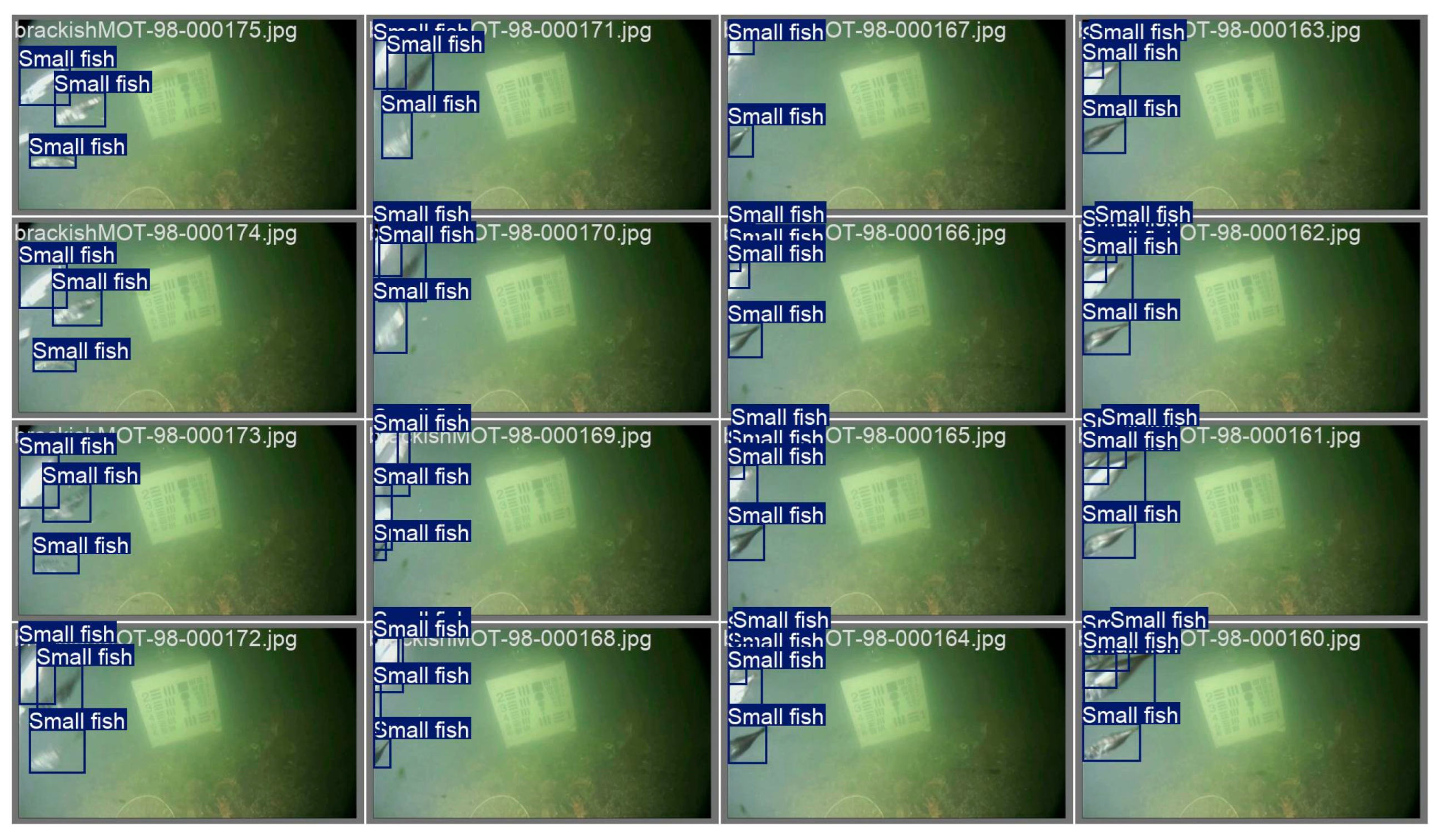
To evaluate the performance of the proposed method, experiments were conducted on the BrackishMOT dataset [25]. It contains real underwater video sequences captured in brackish and visually degraded environments. These scenes include turbidity, low contrast, background interference, and densely distributed aquatic organisms, which are consistent with the visual challenges targeted in this study. In addition, the dataset provides bounding-box annotations for six coarse organism categories, including fish, small fish, crab, shrimp, starfish, and jellyfish, making it suitable for evaluating multi-class underwater object detection rather than single-species fish detection.

(1) Experimental environment

The experiments were implemented using the YOLO11n model within the Ultralytics (v8.3.55) framework. The hardware platform comprised an Intel Core i5-11400H CPU, 16 GB RAM, and an NVIDIA GeForce RTX 3050 GPU (4 GB VRAM). The software stack included Python 3.8.12, PyTorch 1.9.0, CUDA 11.1, and cuDNN 8.0.5, running on NVIDIA driver 470.141.03. To enhance computational efficiency, automatic mixed-precision (AMP) was employed for memory optimization. The entire environment was managed via Conda to ensure dependency consistency and experimental reproducibility.

(2) Experimental setup

The main parameter settings used in this experiment are listed in

Table 1. Training and Evaluation Settings.

Category	Parameter Name	Parameter Value
Data augmentation	Mosaic probability	1.0
	Translation scale	0.1
	Scaling Ratio	0.5
	Flip probability	0.5
	HSV augmentation	True
Training	Initial learning rate	0. 01
	Number of epochs	100
	Batch size	16
	Exponential moving average (EMA)	Enabled
	Weight decay	5 × 10−4
	Momentum	0.937
	Image size	640 × 640
	Mixed precision training	Enabled
	Warm-up epoch	3
	Number of workers	8
	Early stopping patience	50
Inference	Image size	640 × 640
	Confidence threshold	0.3
	NMS threshold	0.7

. Specifically, the HSV color space transformation parameters are set as follows: the hue offset range is 0.015, the saturation adjustment range is 0.7, and the brightness adjustment range is 0.4.

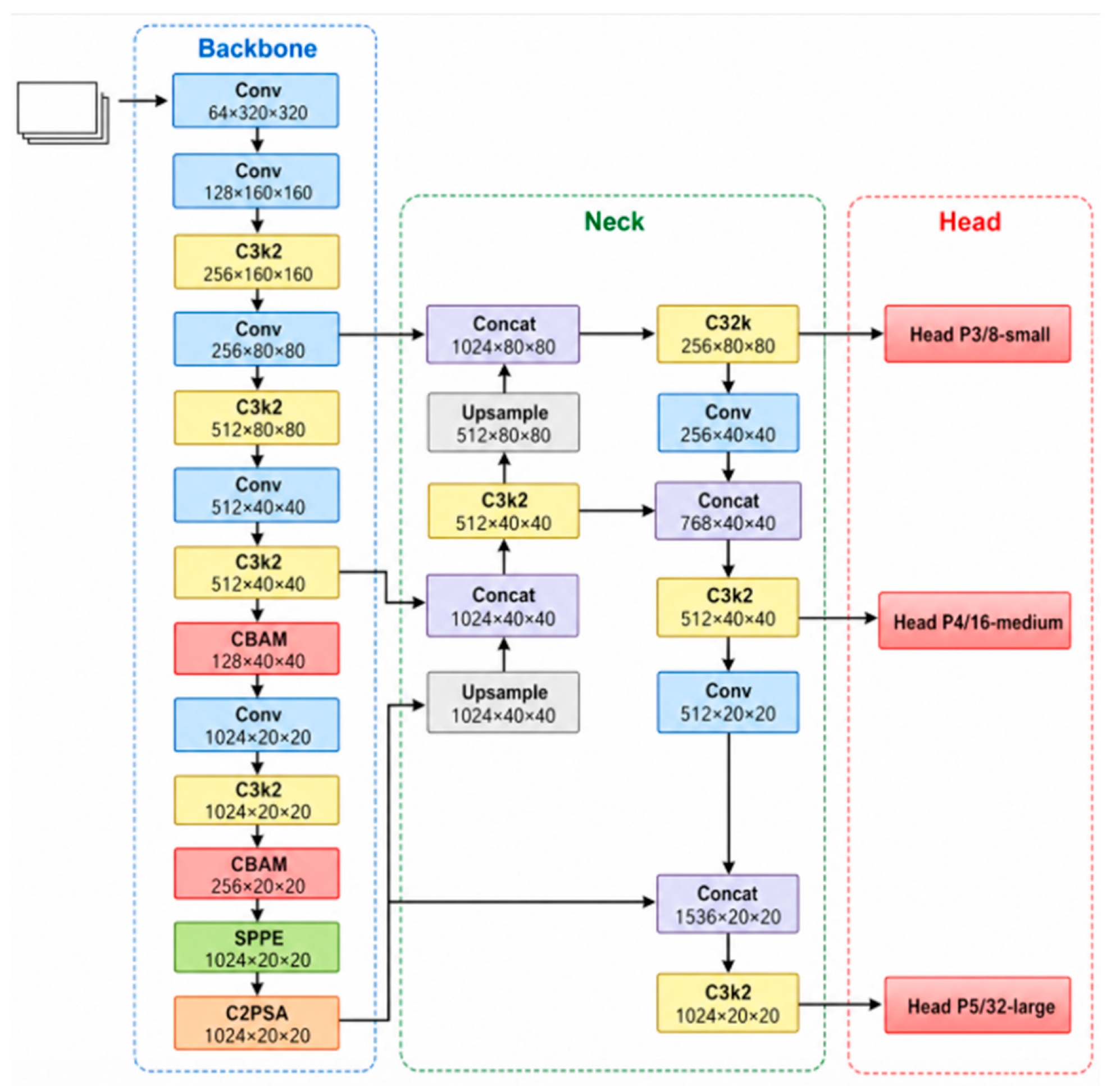
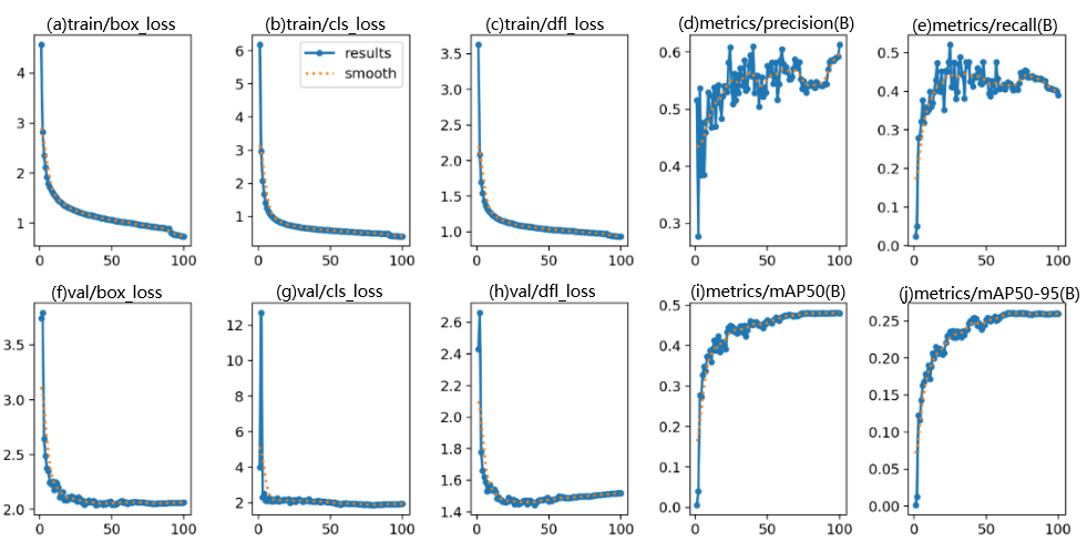
The proposed marine organism detection model, which incorporates multi-scale attention into the YOLO11n architecture, was trained on the BrackishMOT dataset for 100 epochs [25].

When the batch size is set to 16, the peak GPU memory usage reaches 3.2 GB, which is close to the hardware limit of 4 GB memory capacity of the NVIDIA GeForce RTX 3050 graphics card. The relationship between the batch size and the learning rate follows a linear scaling rule:

$${\eta }_{\mathrm{eff}}={\eta }_{\mathrm{base}}\times {\displaystyle \frac{batch}{64}}$$

(11)

where η_base is the base learning rate, η_eff is the effective learning rate, and batch is the number of data samples processed simultaneously during one forward propagation and one backpropagation during the training process.

When the batch size is scaled by a factor of k, the base learning rate is adjusted proportionally to maintain a comparable gradient noise scale. Although this linear scaling rule was originally proposed for large-batch distributed training, it is used here as a practical guideline for adjusting the learning rate under different batch-size settings. Furthermore, early stopping was used to prevent overfitting. The validation mAP was monitored with a patience value of 10, meaning that training was stopped if no improvement was observed for 10 consecutive epochs. The system automatically saves the current optimal weights and terminates the training when the fluctuation of the validation indexes in 10 consecutive epochs is less than ±0.15%. The strategy incorporates the exponentially weighted moving average (EWMA) algorithm to smooth the validation curve, effectively avoiding the misjudgment caused by local fluctuations.

3.2. Data Split, Class Distribution, and Dataset Analysis

The class distributions of the predefined training and validation subsets were counted from the annotation files. The training subset contains 10,999 annotated label files and 34,692 object instances, while the validation subset contains 3018 annotated label files and 14,670 object instances. The class-level instance counts are summarized in

Table 2. Class distribution of BrackishMOT training and validation subsets.

Class	Training Instances	Validation Instances	Total Instances
Fish	2824	497	3321
Crab	9577	3078	12,655
Shrimp	522	26	548
Starfish	6793	1586	8379
Small fish	14,459	9363	23,822
Jellyfish	517	120	637
Total	34,692	14,670	49,362

.

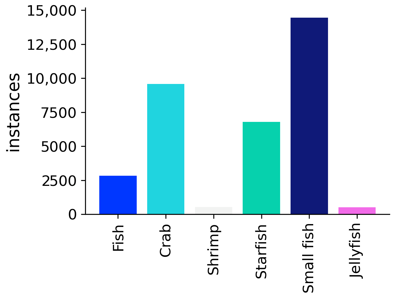
The BrackishMOT dataset exhibits a clear long-tailed class distribution, as illustrated in Figure 3. Small fish accounts for the largest number of annotated instances, with 23,822 instances, followed by Crab with 12,655 instances and Starfish with 8379 instances. Fish contains 3321 instances, whereas Jellyfish and Shrimp are substantially underrepresented, with only 637 and 548 instances, respectively. This imbalance is also reflected in the validation subset. Such a long-tailed distribution may bias the model toward data-abundant categories and reduce the stability of performance estimation for rare categories.

Regarding the class-imbalance issue, the main experiments retained the original class distribution of BrackishMOT. Standard YOLO data augmentations, including Mosaic, translation, scaling, flipping, and HSV color-space augmentation, were applied consistently to all classes. No additional random frame-level re-splitting was performed.

(1) Spatial characterization

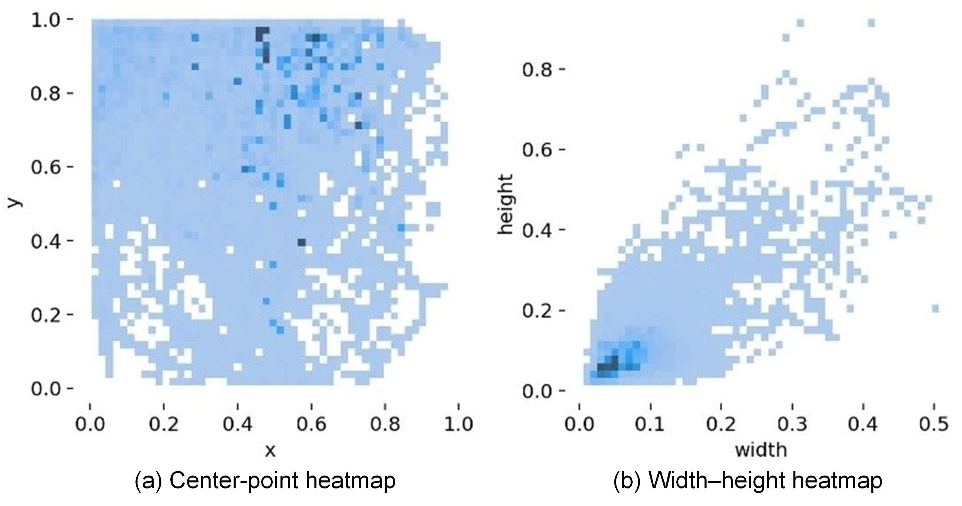
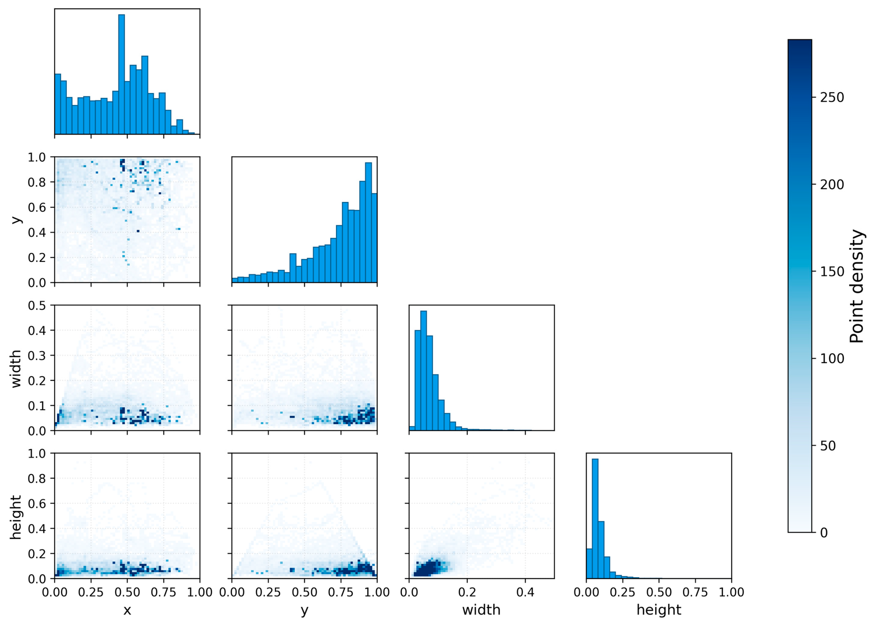
Figure 4 shows the results of the spatial characterization of the dataset, where the spatial distribution is represented by a heat map (x-y coordinate scatter plot).

As can be seen from Figure 4, the target object shows a relatively uniform distribution pattern in the image space, covering the entire image area (normalized coordinate range of 0.0–1.0). This distribution feature indicates that the dataset has good spatial representativeness, which is conducive to the model learning the target features at different locations.

From the width–height distribution graph in Figure 4, it can be observed that the geometric features of the target objects show the following patterns: in terms of size distribution, most of the target objects are concentrated in smaller size ranges, and the width and height are mainly distributed in the normalized range of 0.0–0.4, which is in line with the characteristics of small and medium-sized targets that are dominant in the task of detecting marine organisms; in terms of the aspect ratio features, the target objects show a diverse aspect ratio distribution, indicating that the dataset contains marine organisms with different morphologies, which helps to improve the generalization ability of the model.

(2) Characterization of geometric distribution

Figure 5 shows the results of the statistical analysis of the geometric features of the target frames in the dataset.

The statistical analysis of the geometric features in Figure 5 shows that the dataset has good spatial distribution characteristics and dimensional diversity. In terms of positional distribution, both the x-coordinate and y-coordinate show nearly uniform distribution, and the edge histogram shows smooth coordinate distribution without obvious aggregation or blank area, which confirms the good coverage of the target in the image space. In terms of size distribution, both width and height show right-skewed distribution characteristics, with the peak of width concentrated in the range of 0.0–0.2, and the height of most targets is less than 0.4. This distribution pattern is consistent with the actual needs of the marine life detection task, and highlights the importance of accurate detection of small-sized targets. Correlation analysis shows that there is a positive but not completely linear correlation between width and height, indicating that the dataset contains a variety of morphologically proportional target objects, while the position coordinates do not show a strong correlation with the size parameter, indicating that the target size is relatively independent of its position in the image, and these features together constitute a balanced and representative marine organism detection dataset.

Based on the above statistical analysis, the dataset is suitable for evaluating underwater multi-scale detection because target centers cover a wide image area, most bounding boxes fall within small to medium size ranges, and the aspect ratios vary across organism categories. However, the dataset should not be regarded as class-balanced. The long-tailed class distribution is therefore explicitly considered in the category-wise evaluation and discussion, rather than being hidden by the overall mAP value.

3.3. Model Training Results

Figure 6 illustrates the loss function and evaluation metric changes during training.

Figure 6 shows the training process and convergence behavior of the proposed model. The model was trained from scratch using the YOLO11n architecture defined by the YAML configuration file, rather than being initialized from pretrained weights. The training losses gradually decreased and the validation metrics stabilized in the later epochs, indicating stable convergence under the current training settings.

3.4. Ablation Experiments

Ablation experiments were designed to evaluate the contribution of each individual component to the overall performance. Four configurations were tested:

(1)

Baseline: The original YOLO11n model without any enhancements, used as a performance benchmark.

(2)

YOLO11n + CBAM: The CBAM is introduced alone to assess the impact of the attention mechanism on detection performance.

(3)

YOLO11n + CIoU Loss: The original IoU-based loss function is replaced with the CIoU loss to evaluate its effect on bounding box regression accuracy.

(4)

YOLO11n + CBAM + CIoU Loss: All improvement strategies are applied simultaneously to form the final optimized model.

Through this systematic experimental design, the independent contributions of each improvement component as well as their synergistic effects can be quantitatively assessed, providing a scientific basis for model optimization.

Table 3. Model performance for different optimizations.

Experimental Setup	GFLOPs	mAP@0.5	mAP@0.5:0.95	Precision	Recall
Baseline	6.4	0.465	0.248	0.555	0.431
+CBAM	7.2	0.472	0.253	0.563	0.451
+CIoU Loss	6.4	0.477	0.251	0.582	0.473
+CBAM + CIoU Loss	7.2	0.481	0.260	0.614	0.482

demonstrates the results of model performance under different optimization strategies.

In Table 3, mAP@0.5 denotes the mAP at an IoU threshold of 0.5, while mAP@0.5:0.95 is a stricter metric averaged over IoU thresholds from 0.50 to 0.95. The GFLOP reports the computational cost under an input size of 640 × 640. Since the CIoU loss function only modifies the training objective and does not change the inference architecture, the YOLO11n + CIoU Loss configuration has the same GFLOPs as the baseline model. After introducing CBAM, GFLOPs increase from 6.4 to 7.2. Meanwhile, the number of parameters increases only slightly from 2.591 M to 2.596 M, corresponding to an increase of approximately 0.19%. Therefore, the proposed model improves detection performance with a limited increase in parameter count and a moderate increase in computational cost.

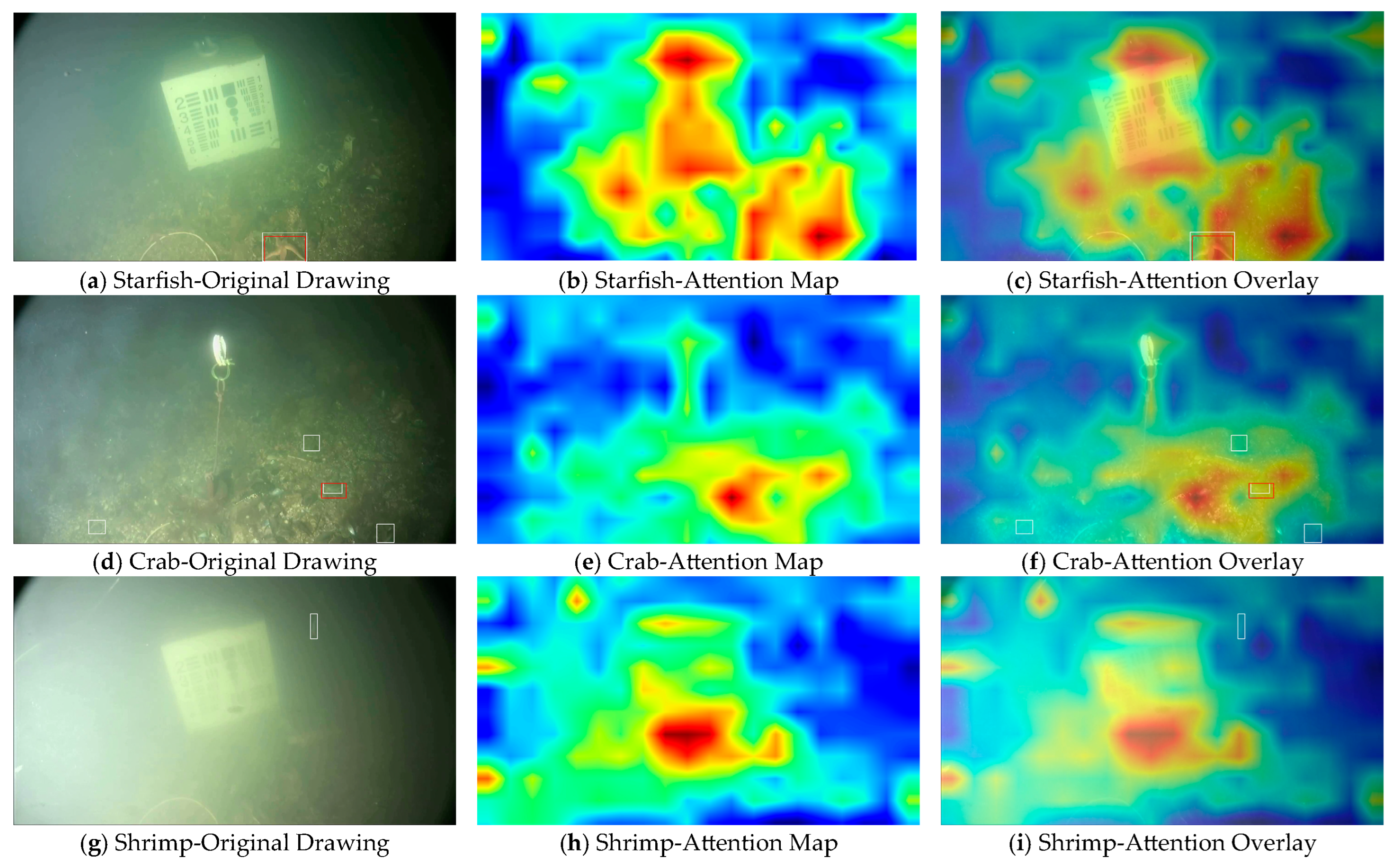
Compared with the baseline YOLO11n model, introducing the CBAM attention module increased mAP@0.5 from 0.465 to 0.472, corresponding to a relative improvement of 1.5%. Precision increased from 0.555 to 0.563, and recall increased from 0.431 to 0.451. These results suggest that CBAM helps the model focus more effectively on informative target regions in complex underwater scenes.

When the CIoU loss function was used, mAP@0.5 increased from 0.465 to 0.477, corresponding to a relative improvement of 2.6%. The mAP@0.5:0.95 value also increased from 0.248 to 0.251, indicating a modest improvement in bounding-box localization under stricter IoU thresholds.

After introducing the CBAM, the model parameters increased from 2,591,010 to 2,595,878, an increase in only 4868 parameters, or approximately 0.19%. Meanwhile, the ablation experiment showed that mAP@0.5 improved from 0.465 to 0.472, precision from 0.555 to 0.563, and recall from 0.431 to 0.451, suggesting that CBAM improves feature representation with limited additional model complexity.

The complete model, which combines CBAM and CIoU loss, achieved the highest overall performance among the tested configurations. Specifically, mAP@0.5 reached 0.481, representing a relative improvement of 3.4% over the baseline model. The mAP@0.5:0.95 value increased from 0.248 to 0.260, corresponding to a relative improvement of 4.8%. Precision and recall also increased to 0.614 and 0.482, respectively. The consistent improvements across the evaluated metrics indicate that the proposed optimization strategy has a positive effect on detection performance. This result suggests that the combined use of CBAM and CIoU loss improves the model’s bounding-box localization and overall detection performance.

To determine the optimal insertion positions for the Convolutional Block Attention Module (CBAM), a series of ablation experiments were conducted. Considering that different feature map resolutions capture varying levels of spatial and semantic information, we evaluated the integration of CBAM after the 80 × 80, 40 × 40, and 20 × 20 feature layers, as well as after all three feature layers respectively. The results are summarized in

Table 4. Ablation experiment on CBAM insertion positions.

CBAM Insertion Position	mAP@0.5	Recall	Precision
After 20 × 20 backbone layer	0.433	0.487	0.493
After 40 × 40 backbone layer	0.444	0.429	0.553
After 80 × 80 backbone layer	0.436	0.423	0.544
After 80 × 80, 40 × 40, and 20 × 20 backbone layers	0.438	0.403	0.553
Proposed setting	0.472	0.451	0.563

.

The results show that the 40 × 40 insertion achieved the highest mAP@0.5 among the single-layer settings, suggesting that mid-level features are particularly useful for detecting small or blurred marine organisms because they retain spatial and edge information while containing more discriminative semantic cues than the shallow 80 × 80 layer. The 20 × 20 insertion produced a relatively high recall, but its lower precision indicates that high-level semantic features alone are less stable for separating targets from complex underwater backgrounds.

When CBAM was inserted into all three feature scales, mAP@0.5 reached 0.438 and recall decreased to 0.403, indicating that adding attention modules indiscriminately does not necessarily improve detection. Excessive attention constraints may suppress useful low-level details or amplify background interference. Therefore, the final 40 × 40 + 20 × 20 setting was adopted to balance mid-level spatial detail enhancement and high-level semantic feature refinement. This ablation experiment provides the empirical basis for the selected CBAM insertion positions.

3.5. Comparative Experiments

Three recent YOLO-based underwater detection models, MAS-YOLOv11 [22], AquaYOLO [23], and Mobile-YOLO [24], were included in the comparison due to their focus on underwater image degradation, multi-scale feature representation, and efficient deployment in aquatic object detection tasks.

All compared models were evaluated under the same BrackishMOT data protocol and evaluation metrics used for the proposed model.

Table 5. Comparative experiments of different detection models.

Model	mAP@0.5	mAP@0.5:0.95	Precision	Recall
Mobile-YOLO	0.398	0.216	0.562	0.389
MAS-YOLOv11	0.327	0.156	0.479	0.303
AquaYOLO	0.374	0.194	0.558	0.346
Ours	0.481	0.260	0.614	0.482

demonstrates the results of the performance comparison of different models on the marine organism detection task. The best results are highlighted in bold.

As shown in Table 5, the proposed model achieves the highest mAP@0.5 (0.481), recall (0.482), and precision (0.614). These results indicate that the combined CBAM and CIoU strategy provides stronger adaptation to the BrackishMOT multi-class underwater detection task than the selected recent aquatic/underwater YOLO variants.

To further examine whether the performance gain was specifically associated with the selected attention design, additional experiments were conducted by replacing CBAM with other representative attention mechanisms using the proposed 40 × 40 and 20 × 20 insertion positions while keeping the same training protocol. The results are presented in

Table 6. Comparison of different attention mechanisms at the same insertion positions.

Model	Params (M)	GFLOPs	Precision	Recall	mAP@0.5	mAP@0.5:0.95
YOLO11n baseline	2.591	6.4	0.555	0.431	0.465	0.248
+CBAM	2.596	7.2	0.563	0.451	0.472	0.253
+C2PSA_MSDA	46.132	105.7	0.519	0.401	0.399	0.222
+SE	3.440	10.8	0.496	0.347	0.354	0.182
+C2f_LSKA_Attention	2.855	6.7	0.509	0.382	0.383	0.194

. The best results are highlighted in bold.

As shown in Table 6, CBAM achieves the highest mAP@0.5 and mAP@0.5:0.95 among the tested attention mechanisms while introducing only a small increase in parameters. In contrast, C2PSA_MSDA substantially increases the parameter count and GFLOPs but does not improve detection accuracy under the current setting. SE and C2f_LSKA_Attention also show lower performance than CBAM. These results suggest that CBAM provides a better balance between feature enhancement and model complexity for the BrackishMOT underwater detection task.

In addition to the attention-module comparison, we further evaluated different bounding-box regression losses to justify the use of CIoU in the proposed model. The same YOLO11n baseline architecture and training protocol were used, and only the bounding-box regression loss was changed. The results are shown in

Table 7. Comparison of different bounding-box regression losses on BrackishMOT.

Loss Setting	Precision	Recall	mAP@0.5	mAP@0.5:0.95
IoU	0.555	0.431	0.465	0.248
GIoU	0.510	0.327	0.357	0.186
DIoU	0.521	0.334	0.347	0.179
CIoU	0.582	0.473	0.477	0.251

. The best results are highlighted in bold.

Table 7 shows that CIoU achieves the best overall performance among the tested loss settings, with an mAP@0.5 of 0.477 and an mAP@0.5:0.95 of 0.251. Compared with IoU, GIoU, and DIoU, CIoU provides more stable improvements across precision, recall, and mAP metrics. This may be attributed to the fact that CIoU jointly considers overlap area, center distance, and aspect ratio, which is beneficial for handling small and irregularly shaped marine organisms.

3.6. Cross-Dataset Evaluation

To evaluate the generalization ability of the proposed method, we further conduct cross-dataset experiments on the DePondFi dataset [29]. The results are shown in

Table 8. Cross-dataset results on the DePondFi underwater fish detection dataset.

Experimental Setup	Params (M)	Precision	Recall	mAP@0.5	mAP@0.5:0.95
Baseline	2.582	0.870	0.762	0.854	0.456
+CBAM	2.582	0.875	0.748	0.856	0.460
+CIoU Loss	2.587	0.852	0.771	0.857	0.461
+CBAM + CIoU Loss	2.587	0.865	0.769	0.859	0.463

. The best results are highlighted in bold.

The consistent improvements across datasets demonstrate that the proposed method exhibits good generalization ability.

4. Discussion

4.1. Category-Wise Performance and Class Imbalance

The category-wise results reveal that the proposed model performs unevenly across different organism classes, mainly due to the long-tailed class distribution of the BrackishMOT dataset.

Table 9. Detection accuracy of different types.

Class	mAP@0.5	Precision	Recall
Fish	0.564	0.613	0.499
Crab	0.141	0.424	0.126
Shrimp	0.015	0.0468	0.374
Starfish	0.678	0.812	0.465
Small fish	0.677	0.739	0.599
Jellyfish	0.808	0.802	0.775

shows the model’s recognition performance for different classes of marine organisms in the dataset.

Table 9 indicates that the model performs unevenly across categories. The strongest results are obtained for Jellyfish (mAP@0.5 = 0.808, precision = 0.802, recall = 0.775), Starfish (mAP@0.5 = 0.678), and Small fish (mAP@0.5 = 0.677). The highest performance for Jellyfish is likely related to its distinctive visual appearance in the images. Although Jellyfish has a relatively small number of instances, its translucent body, rounded outline, and relatively coherent texture provide recognizable visual cues that distinguish it from benthic backgrounds. Compared with Shrimp and Crab, which are often small, low-contrast, or camouflaged with seabed structures, Jellyfish tends to present a more separable silhouette and a clearer region-level appearance. These characteristics allow the attention module to emphasize target-related spatial regions more consistently, which may explain why Jellyfish achieves the strongest category-level performance despite its limited sample size. Starfish also benefits from relatively stable shape cues, such as its radial morphology and clearer contour, but its recall remains lower than Jellyfish, indicating that its detection is still affected by background variation and partial visibility. These results suggest that the proposed model can extend detection beyond fish-only targets and can recognize some non-fish marine organisms when their visual features are sufficiently distinguishable in the annotated images. Notably, although Jellyfish has a relatively small number of annotated instances, it still achieves the highest category-level performance, which suggests that visual distinctiveness, rather than sample size alone, also plays an important role in detection performance.

However, the category-wise breakdown also shows that the model does not perform uniformly across all organism classes. Shrimp has a very low mAP@0.5 of 0.015 and precision of 0.0468, despite a recall value of 0.374. This result is closely related to its extremely small number of annotated instances, especially in the validation subset, where only 26 shrimp instances are available. Therefore, the performance estimate for Shrimp is likely to be unstable and strongly affected by class scarcity. Crab also performs poorly, with mAP@0.5 = 0.141 and recall = 0.126. Unlike Shrimp, Crab is not a rare category in terms of annotation count, so its weaker performance is more likely associated with visual ambiguity, camouflage with benthic backgrounds, and confusion with rocks, sand, or other seabed structures. These results imply that the proposed architecture improves the feasibility of multi-class marine organism detection, but it should not be interpreted as providing equally reliable detection for all categories. In particular, rare, small, or visually camouflaged organisms remain challenging under the current experimental setting. These observations identify a clear direction for future work, where class-aware strategies, such as targeted augmentation, class-balanced sampling, and class-weighted loss functions, could be explored to improve the detection of underrepresented or visually ambiguous categories.

Figure 7 shows the confusion matrix for the detection of different categories of marine organisms.

As shown in Figure 7, the diagonal elements of the normalized confusion matrix represent the proportion of ground-truth objects in each category that are correctly predicted. Jellyfish shows the strongest category-level performance, which suggests that its translucent but distinctive shape can still provide recognizable visual cues. In contrast, Shrimp and Crab are frequently confused with the background or other benthic structures. For Shrimp, the main difficulty is the extremely small number of annotated instances and its small apparent size. For Crab, the low recall is more likely related to camouflage with sand, rocks, and seabed textures, rather than class frequency alone. Therefore, the error patterns suggest that both data imbalance and visual ambiguity contribute to the category-wise performance gap.

For Small fish, which has the largest number of annotated instances, the remaining errors are likely caused by two factors:

(1)

Motion-induced blur. In underwater video, the rapid movement of small fish may blur body boundaries and reduce fine edge details, making the target less distinguishable from the surrounding background. In this study, the term “turbulent water-column background” refers to visually irregular background textures caused by water movement, suspended particles, and illumination variation. Because blurred fish edges and turbulent background textures may both appear as low-contrast and fuzzy regions, the model may confuse fast-moving small fish with the background.

(2)

Target adhesion triggered by group aggregation. Small fish have strong group behavior characteristics. When multiple individuals overlap or are closely arranged, the bounding box detection algorithm is difficult to accurately segment individual targets, and is prone to misidentifying multiple small fish as a single large target or background noise. In addition, the shadowing effect and illumination changes during group swimming further exacerbate the ambiguity of the target boundary, reducing the model’s recognition accuracy of individual small fish.

Figure 8 shows the F1-Confidence curves for the different categories of marine organisms detected as well as the average curves for all categories.

As shown in Figure 8, the average F1 score across all categories reaches its maximum value of 0.48 at a confidence threshold of 0.183. The Small fish, Starfish, and Jellyfish categories maintain relatively higher F1 scores across a wider confidence range, indicating more stable predictions. In contrast, the F1 curves for Shrimp and Crab remain low, which is consistent with the category-wise results in Table 8 and confirms that these two categories are the main bottlenecks of the current model.

4.2. Visualization and Practical Implications

Minnows make up the largest number in the dataset, and Figure 9 shows a sample display of the minnows that the model recognizes as aggregated.

In Figure 9, the detected small-fish instances are labeled in each image. The text “Small fish” in each bounding box indicates the predicted category. The labeled boxes generally align with visible organisms, suggesting stable localization for this visually distinguishable category. In addition, the sample images contain complex backgrounds and noticeable lighting variations, indicating that the model can support preliminary underwater video screening and organism localization under challenging visual conditions.

Attention in the underwater marine-organism detection task is illustrated using heat-map visualization, as shown in Figure 10.

The first and second rows show representative successful cases for Starfish and Crab, respectively, including the original image, the attention map, and the attention-overlay result. The third row shows a representative failure case for Shrimp. Warmer colors indicate stronger feature responses, whereas cooler colors indicate weaker responses. The Shrimp example illustrates that the model response around the annotated target is weak or spatially displaced, which helps explain the missed detection under small size, low contrast, and background camouflage.

The improved YOLO11n model achieves an overall mAP@0.5 of 48.1%, mAP@0.5:0.95 of 26.0%, precision of 61.4%, and recall of 48.2% on the BrackishMOT validation subset. Since BrackishMOT contains visually degraded brackish-water scenes with turbidity, low contrast, and background interference, these results suggest the model’s potential adaptability to challenging underwater conditions.

The attention visualizations provide qualitative evidence that the model can focus on target-related regions for visually distinguishable categories such as Starfish. In contrast, the much lower performance for Shrimp indicates that attention enhancement alone is not sufficient when the target class is visually subtle, small in size, and severely underrepresented in the training data. This observation motivates several concrete directions for future work. First, Focal Loss or class-weighted loss can be introduced to reduce the dominance of majority classes during training. Second, class-balanced sampling and targeted augmentation can be used to increase the exposure of rare categories such as Shrimp. Third, synthetic sample generation may further enrich the visual diversity of underrepresented classes and improve feature learning for rare marine organisms.

4.3. Limitations and Future Work

Although the proposed multi-scale attention-enhanced YOLO11n model improves overall detection performance, the category-wise Shrimp is severely underrepresented in the BrackishMOT dataset, particularly in the validation subset, which contains only 26 annotated instances. This limited sample size leads to unstable performance estimation and insufficient feature learning. Based on these observations, future work will focus on more targeted improvements. For underrepresented categories such as Shrimp, class-balanced sampling and synthetic data generation will be explored to increase effective training diversity and improve feature learning.

Furthermore, while this study focuses on detection accuracy and ablation analysis, future work will also evaluate computational efficiency and deployment feasibility on embedded platforms to assess real-time applicability in practical underwater monitoring scenarios.

4.4. Application Scope

The proposed object detection method can be incorporated into broader underwater monitoring systems. In real-world applications, detection outputs can serve as inputs to downstream tasks. For example, detected regions can be further analyzed to achieve fine-grained species recognition, while temporal tracking can support population estimation and behavioral analysis.

In its current form, the proposed model is most suitable for two practical scenarios. First, it can support preliminary video screening and relative abundance indexing under standardized underwater survey conditions. In brackish or highly turbid environments where direct visual census is difficult, automated detection can help reduce manual annotation effort and provide a more consistent basis for comparing changes in organism occurrence across time or sites. This use is consistent with video-based survey approaches that rely on standardized image or video observations for monitoring fish assemblages [30]. Second, the lightweight YOLO11n-based architecture is suitable for near-real-time monitoring in aquaculture or fixed-camera underwater observation systems, where rapid detection of organism presence, movement, or spatial distribution can support fisheries and farm management. Similar computer-vision-based fish counting and monitoring systems have been explored for aquaculture and fisheries management applications [31].

Overall, the current model can serve as a preliminary detection and screening tool that supports manual review, relative abundance estimation, and real-time observation in visually challenging underwater environments.

5. Conclusions

In this study, a multi-class marine organism detection using multi-scale attention-enhanced YOLO11n is proposed to address the challenges posed by variable target scales and complex underwater environments in marine organism detection tasks. The method incorporates the CBAM attention mechanism to enhance the extraction of small target features, effectively managing the complexities of underwater environments. Additionally, the CIoU loss function is utilized to optimize bounding box regression, which improves the detection accuracy of multi-scale marine organisms by applying geometric constraints.

The experimental results show that the proposed optimized YOLO11n model achieves performance improvement on the BrackishMOT dataset. Compared to the baseline YOLO11n model, the mAP@0.5 increased from 0.465 to 0.481, marking a 3.4% improvement. The mAP@0.5:0.95 rose from 0.248 to 0.260, reflecting a 4.8% increase. Additionally, accuracy improved from 0.555 to 0.614, a 10.6% enhancement, and the recall rate increased from 0.431 to 0.482, which is an 11.8% gain. This method enhances adaptability to targets with varying morphologies and sizes while maintaining efficient detection speed, effectively identifying and localizing a wide range of marine organism targets.