

An Ensemble Learning for Automatic Stroke Lesion Segmentation Using Compressive Sensing and Multi-Resolution U-Net


Abstract
1. Introduction
- It provides a network to protect the private content of data by utilizing the compressed version of the input medical image.
- The proposed network provides an ensemble approach to train the compressed version of the input image.
- It represents a combination of compressive sensing and an ensemble of parallel learners to extract the stroke lesion.
- It provides a novel ensemble multi-resolution U-shaped network for segmenting the medical stroke CT dataset. The term multi-resolution, as used in this study, describes the convolutional structure of the model in which multiple branches with distinct kernel sizes operate in parallel. This allows the network to extract both fine-grained and coarse-grained spatial features from CT scans, which is particularly beneficial for capturing stroke lesions with varying sizes and textures.
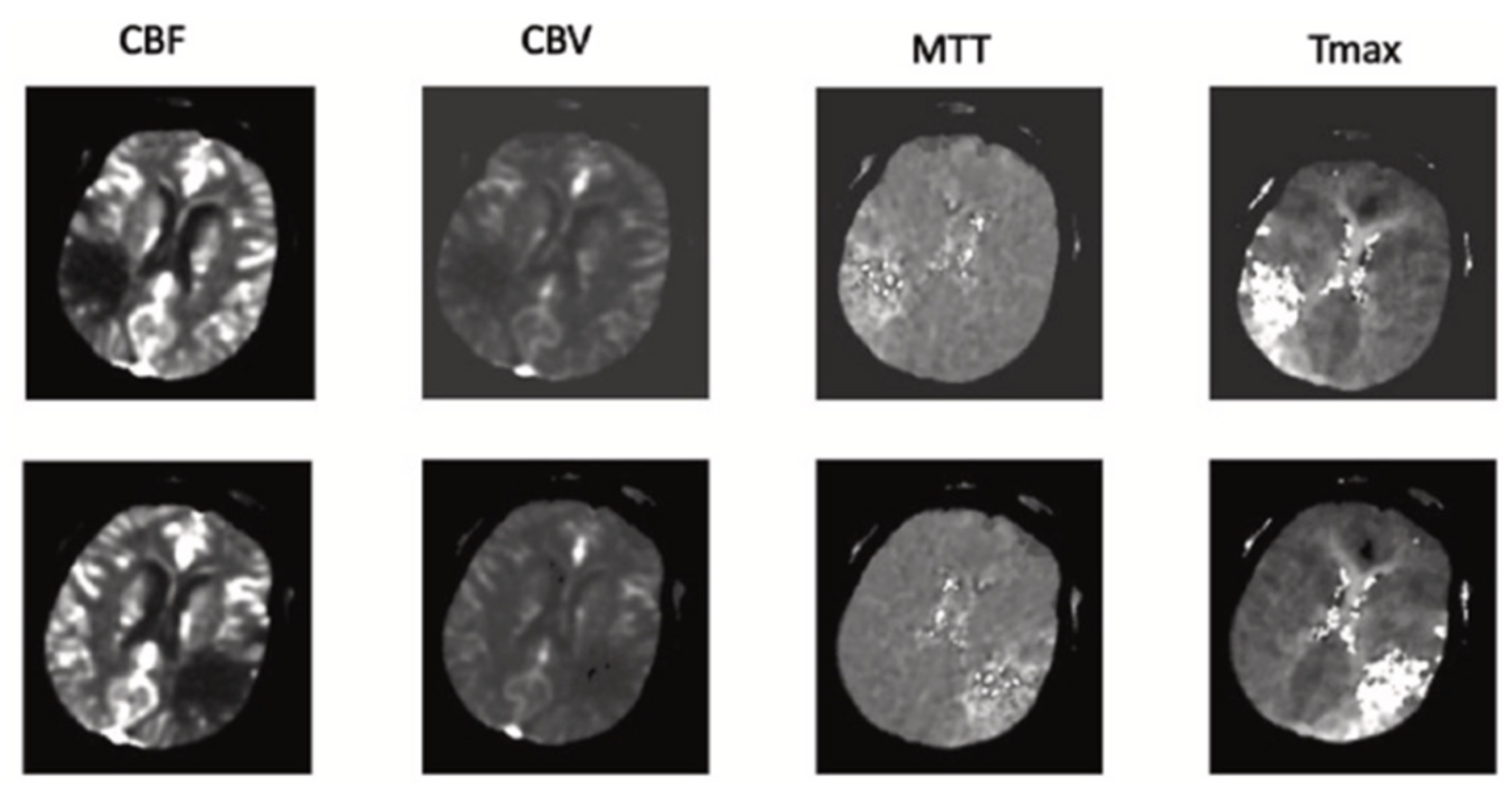
- The proposed network utilizes a channel of perfusion maps, including CBV, CBF, MTT, Tmax, and CT slice, to efficiently extract the stroke lesion.
2. Materials and Methods
2.1. ISLES Database
2.2. CS Theory
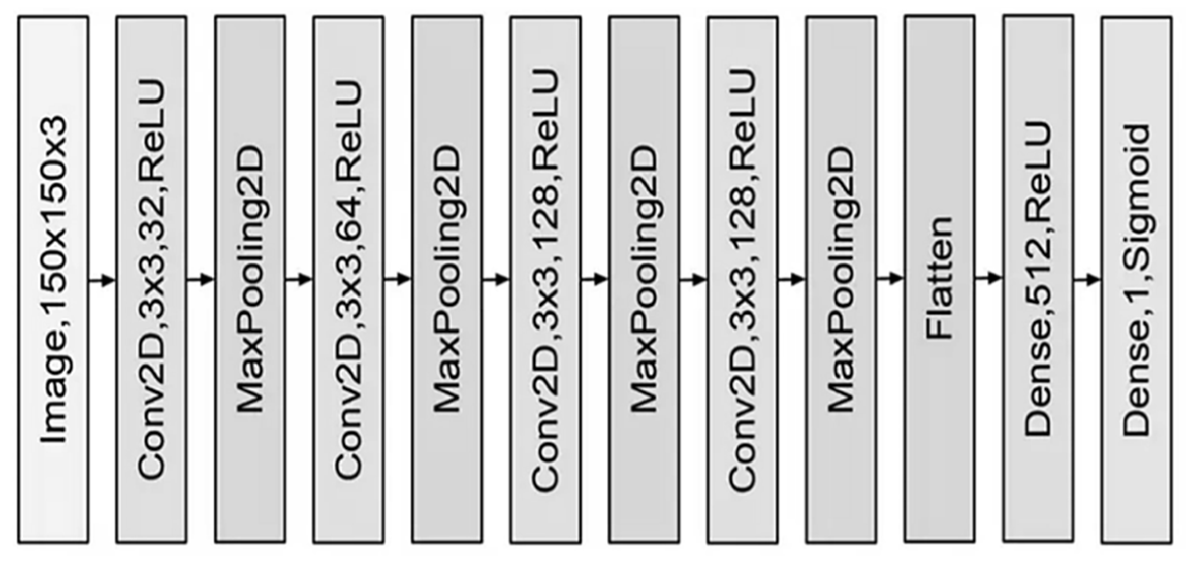
2.3. Convolutional Networks
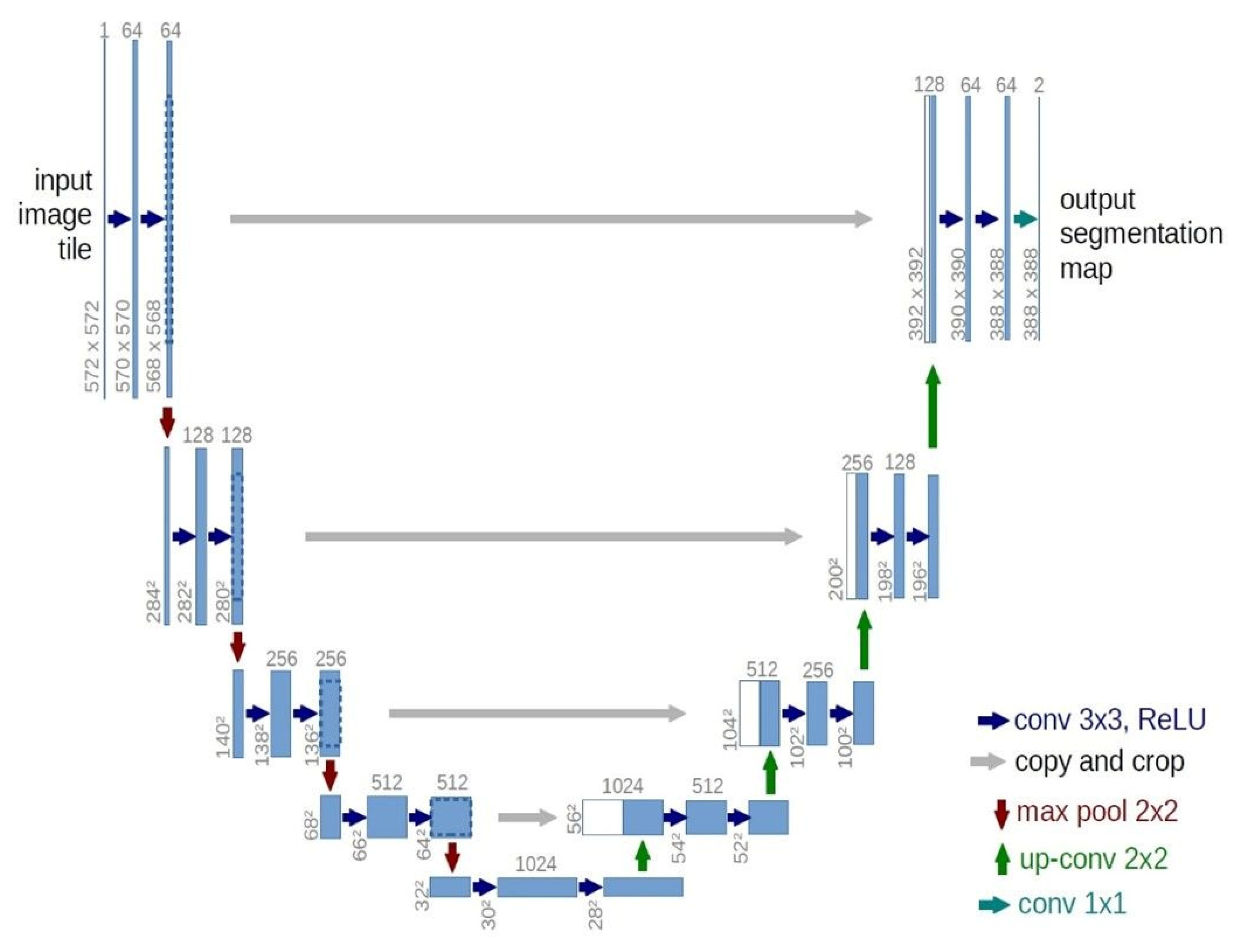
2.4. U-Net
3. Proposed Model
3.1. Pre-Processing of Data
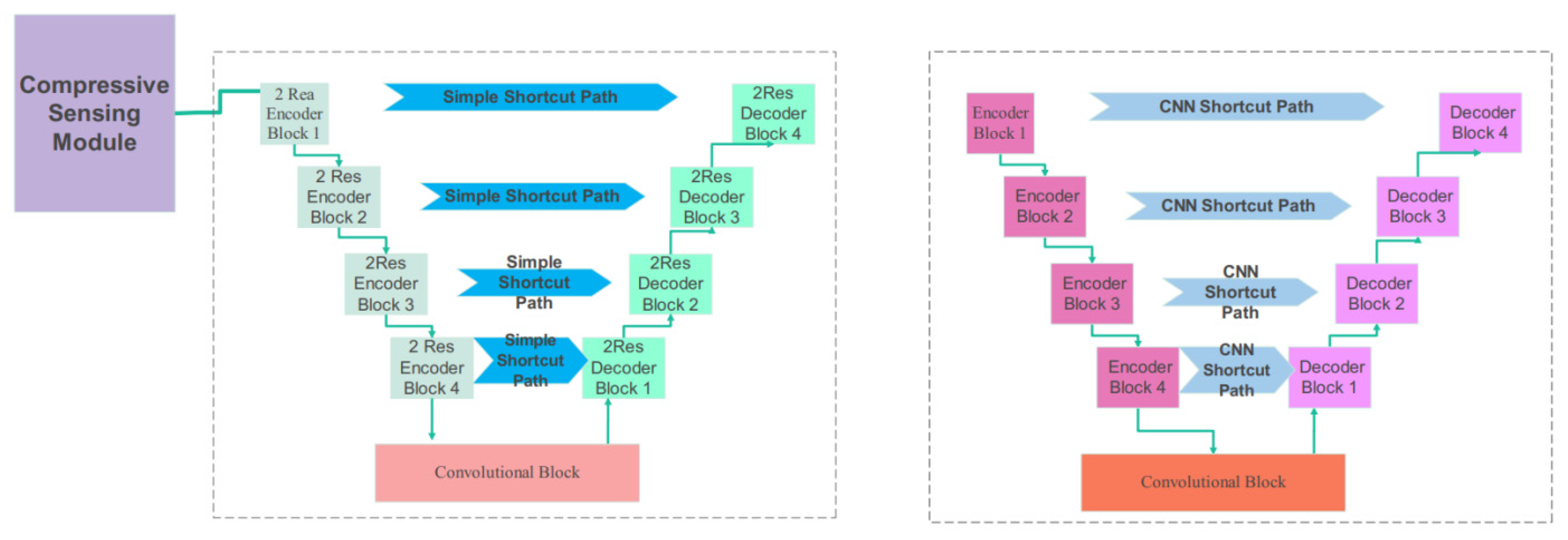
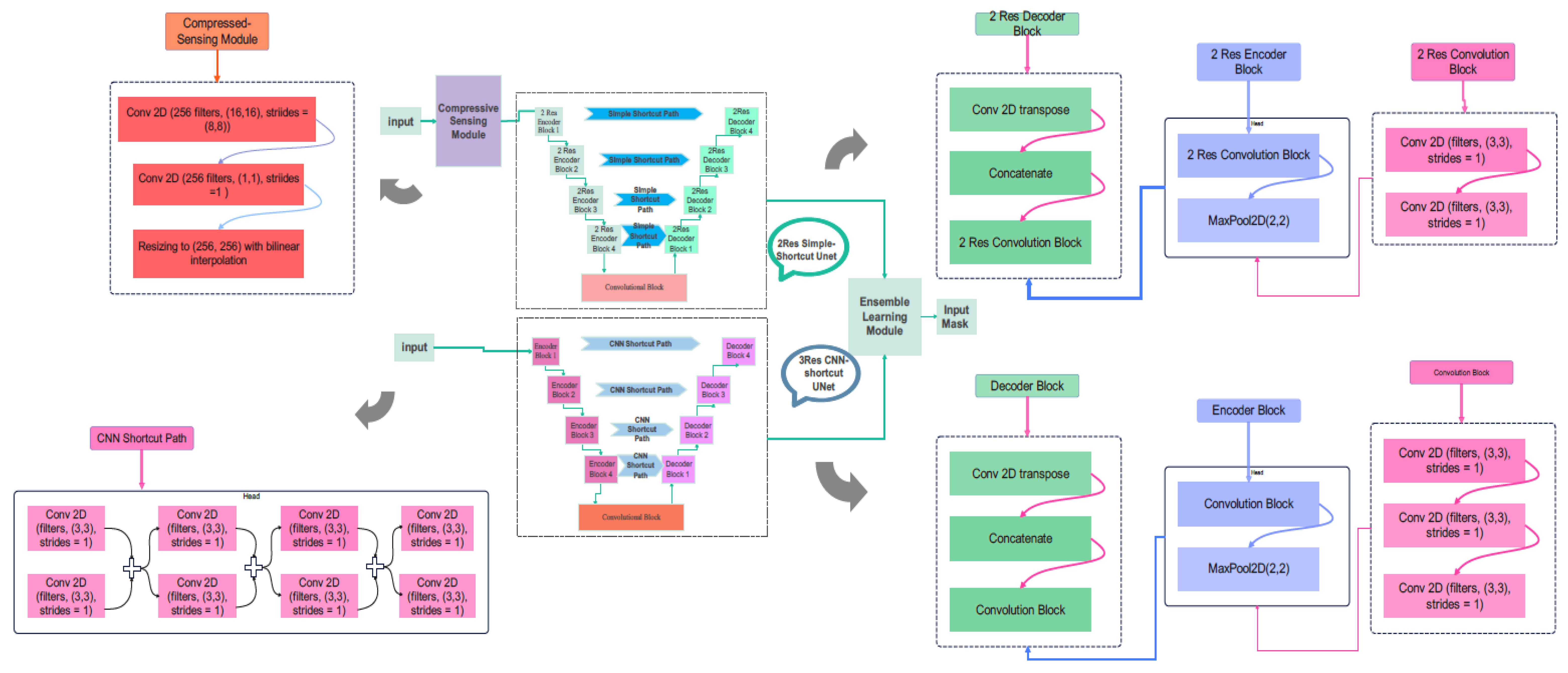
3.2. Proposed Compressive Sensing-Based Ensemble Net (CS-Ensemble Net)
3.3. Proposed CS-Ensemble Net Architecture
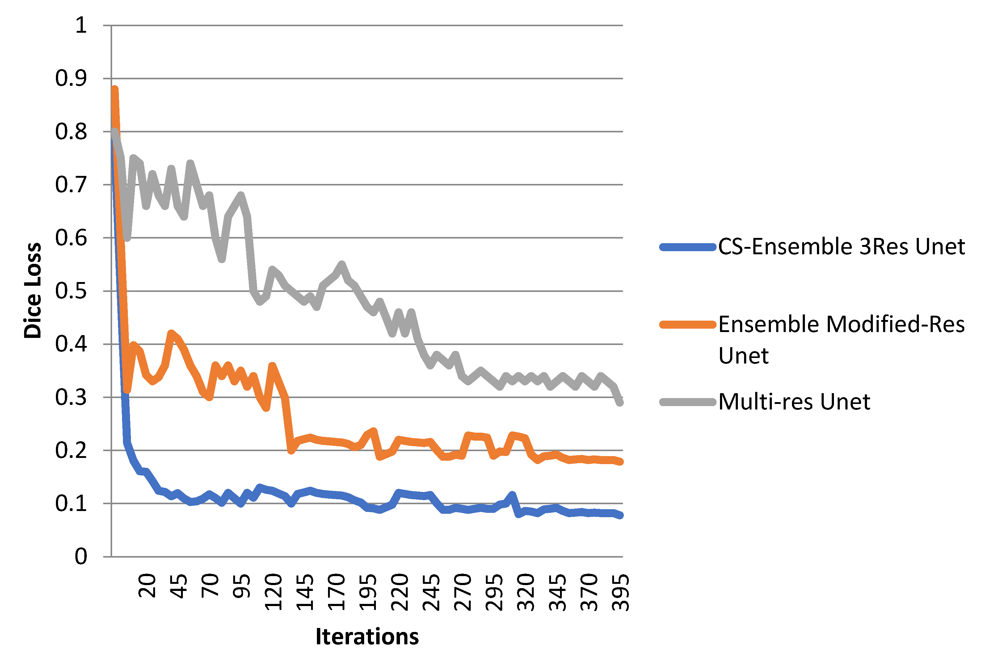
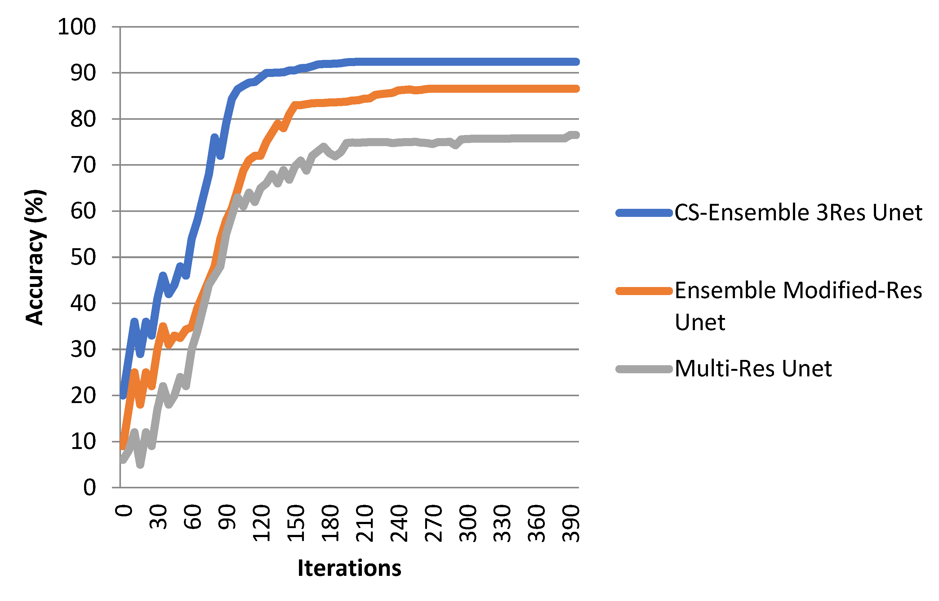
3.4. Training and Evaluation of the CS-Ensemble Net
4. Experimental Results
5. Discussion
6. Conclusions
Author Contributions
Funding
Institutional Review Board Statement
Informed Consent Statement
Data Availability Statement
Conflicts of Interest
References
- Maier, O.; Schröder, C.; Forkert, N.D.; Martinetz, T.; Handels, H. Classifiers for ischemic stroke lesion segmentation: A comparison study. PLoS ONE 2015, 10, e0145118. [Google Scholar] [CrossRef]
- Entezami, M.; Basirat, S.; Moghaddami, B.; Bazmandeh, D.; Charkhian, D. Examining the Importance of AI-Based Criteria in the Development of the Digital Economy: A Multi-Criteria Decision-Making Approach. J. Soft Comput. Decis. Anal. 2025, 3, 72–95. [Google Scholar] [CrossRef]
- Rekik, I.; Allassonnière, S.; Carpenter, T.K.; Wardlaw, J.M. Medical image analysis methods in MR/CT-imaged acute-subacute ischemic stroke lesion: Segmentation, prediction and insights into dynamic evolution simulation models. A critical appraisal. NeuroImage Clin. 2012, 1, 164–178. [Google Scholar] [CrossRef] [PubMed]
- Zhou, Y.; Huang, W.; Dong, P.; Xia, Y.; Wang, S. D-UNet: A dimension-fusion U shape network for chronic stroke lesion segmentation. IEEE/ACM Trans. Comput. Biol. Bioinform. 2019, 18, 940–950. [Google Scholar] [CrossRef] [PubMed]
- Wang, Y.; Katsaggelos, A.K.; Wang, X.; Parrish, T.B. In A deep symmetry convnet for stroke lesion segmentation. In Proceedings of the 2016 IEEE International Conference on Image Processing (ICIP), Phoenix, AZ, USA, 25–28 September 2016; pp. 111–115. [Google Scholar]
- Mitra, J.; Bourgeat, P.; Fripp, J.; Ghose, S.; Rose, S.; Salvado, O.; Connelly, A.; Campbell, B.; Palmer, S.; Sharma, G. Lesion segmentation from multimodal MRI using random forest following ischemic stroke. NeuroImage 2014, 98, 324–335. [Google Scholar] [CrossRef]
- Maier, O.; Wilms, M.; von der Gablentz, J.; Krämer, U.M.; Münte, T.F.; Handels, H. Extra tree forests for sub-acute ischemic stroke lesion segmentation in MR sequences. J. Neurosci. Methods 2015, 240, 89–100. [Google Scholar] [CrossRef]
- Zhang, Y.; Liu, S.; Li, C.; Wang, J. Application of deep learning method on ischemic stroke lesion segmentation. J. Shanghai Jiaotong Univ. (Sci.) 2022, 27, 99–111. [Google Scholar] [CrossRef]
- Qi, K.; Yang, H.; Li, C.; Liu, Z.; Wang, M.; Liu, Q.; Wang, S. In X-net: Brain stroke lesion segmentation based on depthwise separable convolution and long-range dependencies. In Medical Image Computing and Computer Assisted Intervention–MICCAI 2019: 22nd International Conference, Shenzhen, China, 13–17 October 2019; Proceedings, Part III 22; Springer: Berlin/Heidelberg, Germany, 2019; pp. 247–255. [Google Scholar]
- Guerrero, R.; Qin, C.; Oktay, O.; Bowles, C.; Chen, L.; Joules, R.; Wolz, R.; Valdés-Hernández, M.d.C.; Dickie, D.A.; Wardlaw, J. White matter hyperintensity and stroke lesion segmentation and differentiation using convolutional neural networks. NeuroImage Clin. 2018, 17, 918–934. [Google Scholar] [CrossRef]
- Soltanpour, M.; Greiner, R.; Boulanger, P.; Buck, B. In Ischemic stroke lesion prediction in ct perfusion scans using multiple parallel u-nets following by a pixel-level classifier. In Proceedings of the 2019 IEEE 19th International Conference on Bioinformatics and Bioengineering (BIBE), Athens, Greece, 28–30 October 2019; pp. 957–963. [Google Scholar]
- Liu, P. Stroke lesion segmentation with 2D novel CNN pipeline and novel loss function. In International MICCAI Brainlesion Workshop; Springer: Berlin/Heidelberg, Germany, 2018; pp. 253–262. [Google Scholar]
- Dolz, J.; Ben Ayed, I.; Desrosiers, C. In Dense multi-path U-Net for ischemic stroke lesion segmentation in multiple image modalities. In Brainlesion: Glioma, Multiple Sclerosis, Stroke and Traumatic Brain Injuries: 4th International Workshop, BrainLes 2018, Held in Conjunction with MICCAI 2018, Granada, Spain, 16 September 2018, Revised Selected Papers, Part I 4; Springer: Berlin/Heidelberg, Germany, 2019; pp. 271–282. [Google Scholar]
- Wang, G.; Song, T.; Dong, Q.; Cui, M.; Huang, N.; Zhang, S. Automatic ischemic stroke lesion segmentation from computed tomography perfusion images by image synthesis and attention-based deep neural networks. Med. Image Anal. 2020, 65, 101787. [Google Scholar] [CrossRef]
- Talebian, S.; Golkarieh, A.; Eshraghi, S.; Naseri, M.; Naseri, S. Artificial Intelligence Impacts on Architecture and Smart Built Environments: A Comprehensive Review. Adv. Civ. Eng. Environ. Sci. 2025, 2, 45–56. [Google Scholar] [CrossRef]
- Ghnemat, R.; Khalil, A.; Abu Al-Haija, Q. Ischemic stroke lesion segmentation using mutation model and generative adversarial network. Electronics 2023, 12, 590. [Google Scholar] [CrossRef]
- Raju, C.S.P.; Kirupakaran, A.M.; Neelapu, B.C.; Laskar, R.H. Ischemic Stroke Lesion Segmentation in CT Perfusion Images Using U-Net with Group Convolutions, International Conference on Computer Vision and Image Processing; Springer: Berlin/Heidelberg, Germany, 2022; pp. 276–288. [Google Scholar]
- Soltanpour, M.; Greiner, R.; Boulanger, P.; Buck, B. Improvement of automatic ischemic stroke lesion segmentation in CT perfusion maps using a learned deep neural network. Comput. Biol. Med. 2021, 137, 104849. [Google Scholar] [CrossRef] [PubMed]
- Isles Challenge 2018 Ischemic Stroke Lesion Segmentation. Available online: www.isles-challenge.org (accessed on 29 July 2025).
- Lustig, M.; Donoho, D.L.; Santos, J.M.; Pauly, J.M. Compressed sensing MRI. IEEE Signal Process. Mag. 2008, 25, 72–82. [Google Scholar] [CrossRef]
- Bi, D.; Xie, Y.; Ma, L.; Li, X.; Yang, X.; Zheng, Y.R. Multifrequency compressed sensing for 2-D near-field synthetic aperture radar image reconstruction. IEEE Trans. Instrum. Meas. 2017, 66, 777–791. [Google Scholar] [CrossRef]
- Goodfellow, I.; Bengio, Y.; Courville, A. Deep Learning; MIT Press: Cambridge, MA, USA, 2016. [Google Scholar]
- LeCun, Y.; Bengio, Y.; Hinton, G. Deep learning. Nature 2015, 521, 436–444. [Google Scholar] [CrossRef]
- Krithika Alias AnbuDevi, M.; Suganthi, K. Review of semantic segmentation of medical images using modified architectures of UNET. Diagnostics 2022, 12, 3064. [Google Scholar] [CrossRef]
- Jha, S.; Kumar, R.; Priyadarshini, I.; Smarandache, F.; Long, H.V. Neutrosophic image segmentation with dice coefficients. Measurement 2019, 134, 762–772. [Google Scholar] [CrossRef]
- Setiawan, A.W. Image segmentation metrics in skin lesion: Accuracy, sensitivity, specificity, dice coefficient, Jaccard index, and Matthews correlation coefficient. In Proceedings of the 2020 International Conference on Computer Engineering, Network, and Intelligent Multimedia (CENIM), Surabaya, Indonesia, 17–18 November 2020; pp. 97–102. [Google Scholar]
- Alom, M.Z.; Hasan, M.; Yakopcic, C.; Taha, T.M.; Asari, V.K. Recurrent residual convolutional neural network based on u-net (r2u-net) for medical image segmentation. arXiv 2018, arXiv:1802.06955. [Google Scholar]
- Clerigues, A.; Valverde, S.; Bernal, J.; Freixenet, J.; Oliver, A.; Lladó, X. Acute ischemic stroke lesion core segmentation in CT perfusion images using fully convolutional neural networks. Comput. Biol. Med. 2019, 115, 103487. [Google Scholar] [CrossRef]
- Wang, P.; Chen, P.; Yuan, Y.; Liu, D.; Huang, Z.; Hou, X.; Cottrell, G. In Understanding convolution for semantic segmentation. In Proceedings of the 2018 IEEE Winter Conference on Applications of Computer Vision (WACV), Lake Tahoe, NV, USA, 12–15 March 2018; pp. 1451–1460. [Google Scholar]
- Pourasghar, A.; Mehdizadeh, E.; Wong, T.C.; Hoskoppal, A.K.; Brigham, J.C. A Computationally Efficient Approach for Estimation of Tissue Material Parameters from Clinical Imaging Data Using a Level Set Method. J. Eng. Mech. 2024, 150, 04024075. [Google Scholar] [CrossRef]
- Mohammadabadi, S.M.S.; Zawad, S.; Yan, F.; Yang, L. Speed Up Federated Learning in Heterogeneous Environments: A Dynamic Tiering Approach. IEEE Internet Things J. 2024, 12, 5026–5035. [Google Scholar] [CrossRef]
- Sadeghi, S.; Niu, C. Augmenting Human Decision-Making in K-12 Education: The Role of Artificial Intelligence in Assisting the Recruitment and Retention of Teachers of Color for Enhanced Diversity and Inclusivity. Leadersh. Policy Sch. 2024, 1–21. [Google Scholar] [CrossRef]
- Ahmadirad, Z. The Beneficial Role of Silicon Valley’s Technological Innovations and Venture Capital in Strengthening Global Financial Markets. Int. J. Mod. Achiev. Sci. Eng. Technol. 2024, 1, 9–17. [Google Scholar] [CrossRef]
- Golkarfard, A.; Sadeghmalakabadi, S.; Talebian, S.; Basirat, S.; Golchin, N. Ethical Challenges of AI Integration in Architecture and Built Environment. Curr. Opin. 2025, 5, 1136–1147. [Google Scholar]
- Kavianpour, S.; Haghighi, F.; Sheykhfard, A.; Das, S.; Fountas, G.; Oshanreh, M.M. Assessing the Risk of Pedestrian Crossing Behavior on Suburban Roads Using Structural Equation Model. J. Traffic Transp. Eng. (English Ed.) 2024, 11, 853–866. [Google Scholar] [CrossRef]
- Mohaghegh, A.; Huang, C. Feature-Guided Sampling Strategy for Adaptive Model Order Reduction of Convection-Dominated Problems. arXiv 2025, arXiv:2503.19321. [Google Scholar]
- Narimani, P.; Abyaneh, M.D.; Golabchi, M.; Golchin, B.; Haque, R.; Jamshidi, A. Digitalization of Analysis of a Concrete Block Layer Using Machine Learning as a Sustainable Approach. Sustainability 2024, 16, 7591. [Google Scholar] [CrossRef]
- Dehghanpour Abyaneh, M.; Narimani, P.; Javadi, M.S.; Golabchi, M.; Attarsharghi, S.; Hadad, M. Predicting Surface Roughness and Grinding Forces in UNS S34700 Steel Grinding: A Machine Learning and Genetic Algorithm Approach to Coolant Effects. Physchem 2024, 4, 495–523. [Google Scholar] [CrossRef]
- Du, T.X.; Jorshary, K.M.; Seyedrezaei, M.; Uglu, V.S.O. Optimal Energy Scheduling of Load Demand with Two-Level Multi-Objective Functions in Smart Electrical Grid. Oper. Res. Forum 2025, 6, 66. [Google Scholar] [CrossRef]
- Mirbakhsh, A.; Lee, J.; Besenski, D. Development of a Signal-Free Intersection Control System for CAVs and Corridor Level Impact Assessment. Future Transp. 2023, 3, 552–567. [Google Scholar] [CrossRef]
- Amiri, N.; Honarmand, M.; Dizani, M.; Moosavi, A.; Kazemzadeh Hannani, S. Shear-Thinning Droplet Formation Inside a Microfluidic T-Junction Under an Electric Field. Acta Mech. 2021, 232, 2535–2554. [Google Scholar] [CrossRef]
- Afsharfard, A.; Jafari, A.; Rad, Y.A.; Tehrani, H.; Kim, K.C. Modifying Vibratory Behavior of the Car Seat to Decrease the Neck Injury. J. Vib. Eng. Technol. 2023, 11, 1115–1126. [Google Scholar] [CrossRef]
- Mohammadabadi, S.M.S.; Yang, L.; Yan, F.; Zhang, J. Communication-Efficient Training Workload Balancing for Decentralized Multi-Agent Learning. In Proceedings of the 2024 IEEE 44th International Conference on Distributed Computing Systems (ICDCS), Jersey City, NJ, USA, 23–26 July 2024; pp. 680–691. [Google Scholar]
- Mahdavimanshadi, M.; Anaraki, M.G.; Mowlai, M.; Ahmadirad, Z. A Multistage Stochastic Optimization Model for Resilient Pharmaceutical Supply Chain in COVID-19 Pandemic Based on Patient Group Priority. Syst. Inform. Eng. Des. Symp. 2024, 382–387. [Google Scholar] [CrossRef]
- Espahbod, S. Intelligent Freight Transportation and Supply Chain Drivers: A Literature Survey. In Proceedings of the Seventh International Forum on Decision Sciences; Springer: Singapore, 2020; pp. 49–56. [Google Scholar]
- Ahmadirad, Z. Evaluating the Influence of AI on Market Values in Finance: Distinguishing Between Authentic Growth and Speculative Hype. Int. J. Adv. Res. Hum. Law 2024, 1, 50–57. [Google Scholar] [CrossRef]
- Mansouri, S.; Mohammed, H.; Korchiev, N.; Anyanwu, K. Taming Smart Contracts with Blockchain Transaction Primitives: A Possibility? In Proceedings of the 2024 IEEE International Conference on Blockchain (Blockchain), Copenhagen, Denmark, 19–22 August 2024; pp. 575–582. [Google Scholar]
- Sadeghi, S.; Marjani, T.; Hassani, A.; Moreno, J. Development of Optimal Stock Portfolio Selection Model in the Tehran Stock Exchange by Employing Markowitz Mean-Semivariance Model. J. Financ. Issues 2022, 20, 47–71. [Google Scholar] [CrossRef]
- Abbasi, E.; Dwyer, E. The Efficacy of Commercial Computer Games as Vocabulary Learning Tools for EFL Students: An Empirical Investigation. Sunshine State TESOL J. 2024, 16, 24–35. [Google Scholar]
- Ahmadirad, Z. The Role of AI and Machine Learning in Supply Chain Optimization. Int. J. Mod. Achiev. Sci. Eng. Technol. 2025, 2, 1–8. [Google Scholar]
- Sajjadi Mohammadabadi, S.M. From Generative AI to Innovative AI: An Evolutionary Roadmap. arXiv 2025, arXiv:2503.11419. [Google Scholar]


| CT Stroke Lesion | Category | Total Images | Dimension | Number of Train Images | Number of Test Images |
|---|---|---|---|---|---|
| 1 | CBV | 502 | 256*256 | 450 | 52 |
| 2 | CBF | 502 | 256*256 | 450 | 52 |
| 3 | MTT | 502 | 256*256 | 450 | 52 |
| 4 | Tmax | 502 | 256*256 | 450 | 52 |
| 5 | CT | 502 | 256*256 | 450 | 52 |
| Layer | Layer Name | Activation Function | Output Dimension | Size of Kernel | Strides | Number of Kernels | Number of Weights |
|---|---|---|---|---|---|---|---|
| 1 | Convolution 2-D | ReLU | (16, 31, 31, 256) | 16 × 16 | 8 × 8 | 256 | 65,792 |
| 2 | Convolution 2-D | ReLU | (16, 31, 31, 256) | 1 × 1 | 1 × 1 | 256 | 65,792 |
| 3 | Resizing | - | (16, 256, 256, 256) | - | - | - | 0 |
| Total number of parameters | 131,584 |
| Layer | Layer Name | Activation Function | Output Dimension | Size of Kernel | Stride Shape | Number of Kernels | Number of Weights |
|---|---|---|---|---|---|---|---|
| 1 | Conv2-D | ReLU | (16, 256, 256, 64) | 3 × 3 | 1 × 1 | 64 | 640 |
| 2 | Conv2-D | ReLU | (16, 256, 256, 64) | 3 × 3 | 1 × 1 | 64 | 36,928 |
| 3 | MaxPooling 2-D | - | (16, 128, 128, 64) | 64 | 0 | ||
| 4 | Conv2-D | ReLU | (16, 128, 128, 128) | 3 × 3 | 1 × 1 | 128 | 73,856 |
| 5 | Conv2-D | ReLU | (16, 128, 128, 128) | 3 × 3 | 1 × 1 | 128 | 147,584 |
| 6 | MaxPooling 2-D | - | (16, 64, 64, 128) | 128 | 0 | ||
| 7 | Conv2-D | ReLU | (16, 64, 64, 256) | 3 × 3 | 1 × 1 | 256 | 295,168 |
| 8 | Conv2-D | ReLU | (16, 64, 64, 256) | 3 × 3 | 1 × 1 | 256 | 590,080 |
| 9 | MaxPooling 2-D | - | (16, 32, 32, 256) | 256 | 0 | ||
| 10 | Conv2-D | ReLU | (16, 32, 32, 512) | 3 × 3 | 1 × 1 | 512 | 1,180,160 |
| 11 | Conv2-D | ReLU | (16, 32, 32, 512) | 3 × 3 | 1 × 1 | 512 | 2,359,808 |
| 12 | MaxPooling 2-D | - | (16, 16, 16, 512) | 512 | 0 | ||
| 13 | Conv2-D | ReLU | (16, 16, 16, 1024) | 3 × 3 | 1 × 1 | 1024 | 4,719,616 |
| 14 | Conv2-D | ReLU | (16, 16, 16, 1024) | 3 × 3 | 1 × 1 | 1024 | 9,438,208 |
| 15 | Conv2-D transpose | ReLU | (16, 32, 32, 512) | 2 × 2 | 2 × 2 | 512 | 2,097,664 |
| 16 | concatenate | (16, 32, 32, 1024) | - | 0 | |||
| 17 | Conv2-D | ReLU | (16, 32, 32, 512) | 3 × 3 | 1 × 1 | 512 | 4,719,104 |
| 18 | Conv2-D | ReLU | (16, 32, 32, 512) | 3 × 3 | 1 × 1 | 512 | 2,359,808 |
| 19 | Conv2-D transpose | ReLU | (16, 64, 64, 256) | 2 × 2 | 2 × 2 | 256 | 524,544 |
| 20 | concatenate | (16, 64, 64, 512) | - | 0 | |||
| 21 | Conv 2-D | ReLU | (16,64,64,256) | 3 × 3 | 1 × 1 | 256 | 1,179,904 |
| 22 | Conv2-D | ReLU | (16, 64, 64, 256) | 3 × 3 | 1 × 1 | 256 | 590,080 |
| 23 | Conv2-D transpose | ReLU | (16, 128, 128, 128) | 2 × 2 | 2 × 2 | 128 | 131,200 |
| 24 | concatenate | (16, 128, 128, 256) | - | 0 | |||
| 25 | Conv 2-D | ReLU | (16, 128, 128, 128) | 3 × 3 | 1 × 1 | 128 | 295,040 |
| 26 | Conv2-D | ReLU | (16, 128, 128, 128) | 3 × 3 | 1 × 1 | 128 | 147,584 |
| 27 | Conv2-D transpose | ReLU | (16, 256, 256, 64) | 2 × 2 | 2 × 2 | 64 | 32,832 |
| 28 | concatenate | (16, 256, 256, 128) | - | 0 | |||
| 29 | Conv 2-D | ReLU | (16, 256, 256, 64) | 3 × 3 | 1 × 1 | 64 | 73,792 |
| 30 | Conv2-D | ReLU | (16, 256, 256, 64) | 3 × 3 | 1 × 1 | 64 | 36,928 |
| 31 | Conv2-D | ReLU | (16, 256, 256, 1) | 2 × 2 | 2 × 2 | 65 |
| Layer Name | Total Number of Trainable Parameters |
|---|---|
|
Conv2-D Concatenate MaxPooling 2-D Conv2-D Transpose | 84,632,001 |
| Parameters | Search Scope | Optimal Value |
|---|---|---|
| Optimizer of first part | Adam | Adam |
| Cost function of first part | MAE, Dice Loss | Dice Loss |
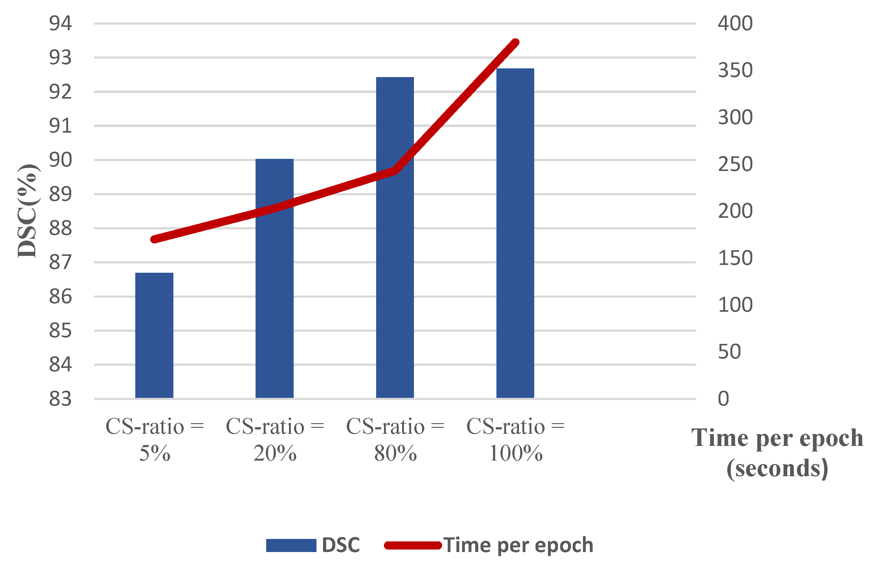
| CS ratio | 5%, 25%, 80%, 100% | 80% |
| Learning rate of first part of Ensemble Net | 0.1, 0.01, 0.001 | 0.001 |
| Shortcut path of second part | Simple, CNN | CNN |
| Optimizer of MA | Adam | Adam |
| Learning rate of second part of Ensemble Net | 0.01, 0.001, 0.0001, 0.00001 | 0.0001 |
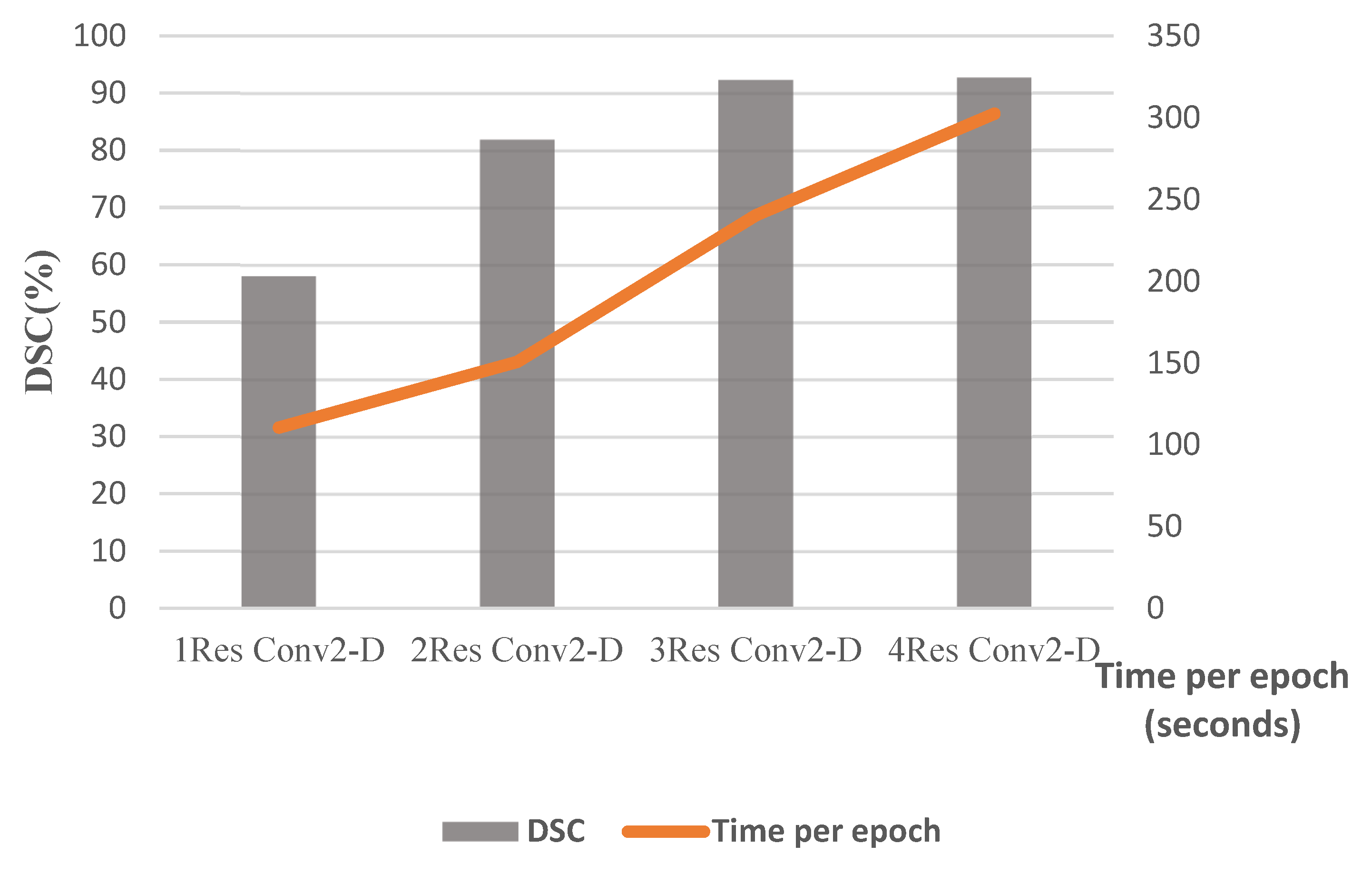
| Number of transposed 2D-convolution layers of decoders | 1, 2, 3, 4 | 3 |
| Number of 2D-convolution layers of encoders | 1, 2, 3, 4 | 3 |
| CTP Mode | Methods | Accuracy (%) | Sensitivity (%) | Dice-Coeff (%) | Mean-IoU (%) |
|---|---|---|---|---|---|
| CBV | MultiresUNet | 73.12 | 70.09 | 71.12 | 65.59 |
| Ensemble Net | 84.03 | 81.95 | 82.23 | 77.84 | |
| CS-Ensemble Net | 89.09 | 86.64 | 87.65 | 84.56 | |
| CBF | MultiresUNet | 70.14 | 68.52 | 68.96 | 63.79 |
| Ensemble Net | 79.96 | 76.89 | 78.56 | 73.84 | |
| CS-Ensemble Net | 85.62 | 84.23 | 84.51 | 82.09 | |
| MTT | MultiresUNet | 71.45 | 69.76 | 70.64 | 63.79 |
| Ensemble Net | 80.62 | 78.89 | 78.96 | 77.59 | |
| CS-Ensemble Net | 87.93 | 85.29 | 86.75 | 83.09 | |
| Tmax | MultiresUNet | 73.43 | 72.44 | 72.69 | 70.86 |
| Ensemble Net | 82.34 | 80.05 | 81.96 | 79.92 | |
| CS-Ensemble Net | 89.34 | 86.91 | 87.73 | 85.64 | |
| [CBV, CBF, MTT, Tmax, CTSlice] | MultiresUNet | 76.52 | 73.09 | 75.12 | 71.19 |
| Ensemble Net | 86.61 | 84.13 | 84.98 | 77.67 | |
| CS-Ensemble Net | 92.43 | 90.14 | 91.66 | 86.16 |
| CS-Ratio | CTP Mode | Accuracy (%) | Sensitivity (%) | Dice-Coeff (%) | Mean-IoU (%) |
|---|---|---|---|---|---|
| 5% | [CBV, CBF, MTT, Tmax, CTSlice] | 86.69 | 85.09 | 85.41 | 81.99 |
| 20% | 90.03 | 87.77 | 88.02 | 86.35 | |
| 80% | 92.43 | 91.30 | 91.83 | 87.82 |
| CTP Mode | Methods | Accuracy (%) | Sensitivity (%) | Dice-Coeff (%) | Mean-IoU (%) |
|---|---|---|---|---|---|
| CBV with noise | MultiresUnet | 76.52 | 74.18 | 75.93 | 73.03 |
| Ensemble Net | 80.15 | 77.29 | 79.02 | 76.04 | |
| CS-Ensemble Net | 85.02 | 83.98 | 83.99 | 84.2 |
Disclaimer/Publisher’s Note: The statements, opinions and data contained in all publications are solely those of the individual author(s) and contributor(s) and not of MDPI and/or the editor(s). MDPI and/or the editor(s) disclaim responsibility for any injury to people or property resulting from any ideas, methods, instructions or products referred to in the content. |
© 2025 by the authors. Licensee MDPI, Basel, Switzerland. This article is an open access article distributed under the terms and conditions of the Creative Commons Attribution (CC BY) license (https://creativecommons.org/licenses/by/4.0/).
Share and Cite
Emami, M.; Tinati, M.A.; Musevi Niya, J.; Danishvar, S. An Ensemble Learning for Automatic Stroke Lesion Segmentation Using Compressive Sensing and Multi-Resolution U-Net. Biomimetics 2025, 10, 509. https://doi.org/10.3390/biomimetics10080509
Emami M, Tinati MA, Musevi Niya J, Danishvar S. An Ensemble Learning for Automatic Stroke Lesion Segmentation Using Compressive Sensing and Multi-Resolution U-Net. Biomimetics. 2025; 10(8):509. https://doi.org/10.3390/biomimetics10080509
Chicago/Turabian StyleEmami, Mohammad, Mohammad Ali Tinati, Javad Musevi Niya, and Sebelan Danishvar. 2025. "An Ensemble Learning for Automatic Stroke Lesion Segmentation Using Compressive Sensing and Multi-Resolution U-Net" Biomimetics 10, no. 8: 509. https://doi.org/10.3390/biomimetics10080509
APA StyleEmami, M., Tinati, M. A., Musevi Niya, J., & Danishvar, S. (2025). An Ensemble Learning for Automatic Stroke Lesion Segmentation Using Compressive Sensing and Multi-Resolution U-Net. Biomimetics, 10(8), 509. https://doi.org/10.3390/biomimetics10080509