Abstract
Remarkable chiral activity is donated to a copper deposit surface by magneto-electrodeposition, whose exact mechanism has been clarified by the three-generation model. In copper deposition under a vertical magnetic field, a macroscopic tornado-like rotation called the vertical magnetohydrodynamic (MHD) flow (VMHDF) emerges on a disk electrode, inducing the precessional motions of various chiral microscopic MHD vortices: First, chiral two-dimensional (2D) nuclei develop on an electrode by micro-MHD vortices. Then, chiral three-dimensional (3D) nuclei grow on a chiral 2D nucleus by chiral nano-MHD vortices. Finally, chiral screw dislocations are created on a chiral 3D nucleus by chiral ultra-micro MHD vortices. These three processes constitute nesting boxes, leading to a limiting enantiomeric excess (ee) ratio of 0.125. This means that almost all chiral activity of copper electrodes made by this method cannot exceed 0.125. It also became obvious that chirality inversion by chloride additive arises from the change from unstable to stable nucleation by the specific adsorption of it.
1. Introduction
In recent years, it has been found that ionic vacancies are produced in solution phases as byproducts of electrode reactions [1,2]. Ionic vacancies are charged particles created to keep the conservations of linear momentum and electricity during electron transfers in electrode reactions. The initially created embryo vacancies are similar to ions isolated in free space, energetically unstable in solution phases. In accordance with the Debye–Hückel theory, ions in solution phases are stabilized by the solvation, surrounded by ionic clouds. At the same time, from the ionic clouds, the solvation energies are liberated, producing entropies around the ions. This is the reason why the activities of ions are less than 1.0. In the same way, the embryo vacancies are also stabilized by the solvation, surrounded by ionic clouds. However, since embryo vacancies are composed of minute free spaces, the liberated solvation energies are not dispersed as heat but used for the dynamic works to enlarge their free-space cores, and stored in the cores. As a result, it is concluded that in the solvation, ionic vacancies do not produce entropies. As shown in Figure 1a,b, a solvated ionic vacancy is a charged free space of the order of nm, surrounded by polarized solvent molecules and an ionic cloud with opposite charges. Though collided by surrounding solvent molecules in a collision time of 10−10 s, a solvated ionic vacancy keeps an intrinsic lifetime of 1 s [3,4], which is, compared with the collision time, extraordinarily long. This result strongly suggests that an ionic vacancy behaves as an iso-entropic particle without entropy production during transfer. Plainly, an ionic vacancy plays a role of an atomic scale lubricant, so that a vacancy layer formed on the electrode provides a free surface without friction, and the viscosity of the layer drastically decreases to zero. Such features have been validated by various experiments [3,4,5,6].
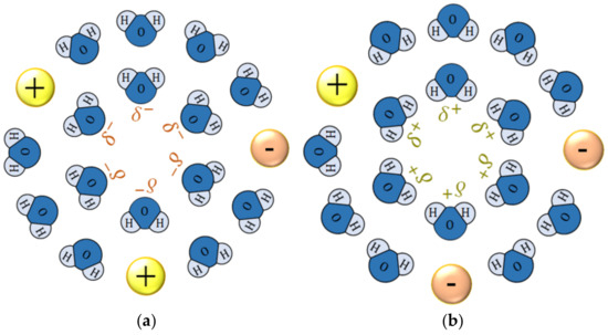
Figure 1.
Solvated ionic vacancies. (a) Negative ionic vacancy. (b) Positive ionic vacancy. H, proton; O, oxygen atom; and , partial polarized charges of water molecules surrounding the free spaces; ⊕, cation; ⊝, anion.
In an electrode reaction under a vertical magnetic field, as shown in Figure 2, a macroscopic tornado-like rotation called the vertical magnetohydrodynamic (MHD) flow (VMHDF) emerges over a disk electrode with a fringe (fringed vertical MHD electrode (fringed-VMHDE)). In the preceding papers [5,6], the processes of the MHD rotation and the resulting mass transfer have been clarified. The electrode surface is covered with ionic vacancies, providing a free surface without friction. A fringed-VMHDF is divided by an upper rotational layer and a lower radial flow layer. The rotation of the upper layer is driven by the Lorentz force, and the radial flow arises from the pressure difference on the fringe of the electrode. By removing the fringe, we will find only a rotating piston-like flow without the radial flow layer.
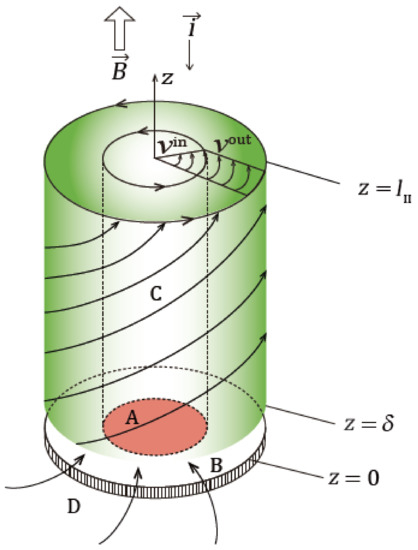
Figure 2.
Schematic of a VMHDF on a fringed-VMHDE [6]. A, copper disk electrode; B, doughnut-shaped fringe of VMHDE; C, rotational-boundary-layer-flow; D, radial-boundary-layer-flow., the thickness of the radial boundary layer (~0.1 mm); , the height of the rotational boundary layer (~several mm); , inner tangential velocity on the electrode; , outer tangential velocity on the fringe; , magnetic flux density; , current density; , -axis. Reproduced with permission from Takagi, S.; Asada, T.; Oshikiri, Y.; Miura, M.; Morimoto, R.; Sugiyama, A.; Mogi, I.; Aogaki, R., Journal of Electroanalytical Chemistry; published by Elsevier B.V., 2022.
Mogi and co-workers have been experimentally clarifying the chirality-emerging processes of copper electrodeposition under VMHDFs [7,8,9,10,11,12,13,14,15,16,17,18]. Chiral deposit films of copper were fabricated by chiral microscopic vortices called micro- and nano-MHD flows, formed on and in vacancy layers, which have chiral activities for enantiomeric reactions of amino acids. By changing the direction of the magnetic field and electrochemical conditions, various modes of chirality emergence are possible. The most important point of this process is that microscopic chiral vortices create chiral screw dislocations with chiral activities. Such chirality of the vortices is caused by the precession from the VMHDF [8,19]. The rotational direction of the VMHDF is determined by the direction of the vertical magnetic field [5,6]; upward and downward magnetic fields provide the anticlockwise (ACW) and clockwise (CW) rotations, respectively. From these experimental results, it is concluded that the rotation of a VMHDF induces chiral precessions of the micro- and nano-MHD flows, which in turn produce chiral screw dislocations with chiral activities. From the hydrodynamic point of view, such microscopic vortices are only permitted in the case of a drastic decrease of viscosity or zero viscosity, i.e., the viscosity of the ordinary solution is too high for them to rotate. However, fortunately, the ionic vacancies mentioned above assist the vortex rotations with zero viscosity.
However, several important problems are still open to us; the scale of the length of a VMHDF (~1 mm) is 107 times as large as that of a screw dislocation (~0.1 nm). The first question is—how are such chiral screw dislocations created by the rotation of the VMHDF despite extremely different scales of length? (Q1). Generally, nucleation in electrodeposition is classified into 2D nucleation of the order of 0.1 mm, 3D nucleation of the order of 0.1 μm, and screw dislocations of the order of 0.1 nm. Therefore, the emergence of the chiral activity would be composed of the three generations of chiral nuclei, i.e., chiral 2D nucleus, chiral 3D nucleus, and chiral screw dislocation. A chiral screw dislocation is created on a chiral 3D nucleus, which in turn grows on a chiral 2D nucleus developing under a VMHDF. These three processes form a nesting-boxes structure. As will be clarified later, based on a simple evidence, the fact that the chiral activity arises from the three generations is validated from both theoretical and experimental aspects. As for 2D and 3D nuclei, the nucleation processes under parallel magnetic fields have been established [20,21,22,23], so in the present papers, we should examine how chiral 2D and 3D nuclei emerge under VMHDF rotations.
The chiral activity of the electrode is estimated by the enantiomeric excess (ee) ratio introduced by Mogi [9,10,11,12,13,14,15,16,17,18]. A characteristic fact derived from the previous experimental results is that the obtained ee ratios are distributed around 0.1. Does such a not-so-high ratio mean the low efficiency of this method? To tell the truth, it is important evidence for the three-generation model.
Furthermore, to receive the precessional motions from VMHDF rotations, vortices must revolve around a vertical axis with the VMHDF, whereas to create chiral nuclei fixed on the electrode, the vortices must keep their positions constant without any transfer. The second question is—how should such incompatible situations concerning the vortices be solved? That is, how do the fixed vortices without revolution receive the precessions from the VMHDF? (Q2).
Since the microscopic vortices are activated from a stationary state in the lower layer, to conserve their total angular momentums, the evolution probabilities of the vortices with ACW rotations must be equal to that of the vortices with CW rotations. Individual vortices have ACW or CW rotation, and adjoining vortices form a pair of vortices with opposite rotations. Even if one of a pair of the vortices receives the precession, due to the continuity of vortex motion, the opposite rotation of the other vortex is also enhanced. If the pair were composed of equivalent vortices with opposite rotations, we could not discriminate the selectivity of the precession, and would always observe achiral activities. To overcome such a contradiction, i.e., for either vortex to receive the precession, we must have two different types of vortices. If both kinds of vortices had similar properties, chirality breakdown would easily occur. The third question is—how are the two kinds of vortices self-organized? How is the precession selectively donated to either of them? (Q3).
From the above Mogi reports [9,10,11,12,13,14,15,16,17,18], the phenomenon that the chiral activity changes with the direction of an applied magnetic field is called “odd chirality”. Namely, the copper films deposited under antiparallel (upward) and parallel (downward) magnetic fields provide D- (CW) and L- (ACW) chiral activities, respectively, which are opposed to the rotational chirality of the VMHDF mentioned above [18]. The fourth question is—why are the chiral activities of the electrode not consistent with the rotational chirality of the VMHDF? (Q4).
Then, Mogi also reported that by adding chloride additives, D-chiral activity changes to L-chiral activity, showing L-activity in both magnetic-field directions (the breakdown of odd chirality) [10,13]. The final and fifth question is—what is the mechanism of such a chirality change? (Q5).
To examine the microscopic processes mentioned above, it is necessary to precisely analyze the vertical MHD flow based on hydrodynamic and MHD theories. Fortunately, in magnetoelectrochemistry, we have already obtained various useful means for the analysis of electrochemical reactions under a magnetic field. Over five decades, many researchers have been struggling to develop magnetoelectrochemistry [24,25,26,27,28,29,30,31,32]. In electrode reactions under magnetic fields, two kinds of forces, i.e., Lorentz force and gradient field force (Kelvin force) appear. The Lorentz force often overwhelms the gradient field force, yielding a macroscopic convection called MHD flow. In accordance with Fahidy [27,28,29], MHD flow decreases the thickness of the diffusion layer, promoting mass transfer in the electrode reaction (MHD effect). As will be mentioned later, such a magnetic field effect on micro-electrodes was, as shown below, theoretically analyzed by Olivier [30,31,32]. Regarding the MHD flow in a channel electrode, called the MHD electrode, the diffusion current equations of the boundary layer flow and viscous flow were proposed by Aogaki [33,34,35].
Mutschke and co-workers examined electrodepositions in cuboid cells under magnetic fields accompanied by 3D convections affected by a gravitational field, which were numerically simulated in various cases [36,37]. Another important aspect of the MHD effect can influence the phase composition of composite metals (Olivier, Alemany, Daltin, Chopart, Hinds, Coey, Zabiński) [38,39,40,41,42,43,44,45,46].
The heterogeneous magnetic field yields magneto-convection by the gradient field force in a paramagnetic solution, enhancing the mass transfer process [47,48,49]. For the MHD effect under magnetic gradient fields, it has been clarified that a superimposed Lorentz force provides more complicated effects to deposit the pattern and composition (Tschulik, Uhlemann, Mutschke, Dunne, Coey) [50,51,52,53,54].
For the analysis of the electrochemical reaction using a micro-disk-electrode under a magnetic field, we can refer to some important achievements as follows: By using a micro-disk-electrode, Olivier established electrochemical impedance spectroscopy in a magnetic field [30,55,56], and at the same time found that the steady-state currents measured under parallel magnetic fields are proportional to , where is the magnetic flux density and is the concentration of the electroactive species. White and coworkers [57,58,59] performed the investigation of magneto-electrochemical effects at ultra-micro-disk electrodes. The magnetic field effects on the limiting (steady-state) current were studied by using cyclic voltammetry in non-aqueous systems containing organic reactants acting as electroactive species. They concluded that the magnetic field effect was attributed to the convective flow caused by the viscous drag of the electrolyte ions accelerated by the magnetic force.
Recently, Mutschke and coworkers studied the electrodeposition of copper on a conically shaped diamagnetic electrode under the influence of a vertical magnetic field [60]. Using magnet arrays of small cylindrical magnets, Dunne and Coey studied deposit patterns of cathodic electrodeposition reflecting the non-uniform magnetic field [51,61].
The MHD electrode proposed by Aogaki was composed of a rectangular channel with two open edges, and a rectangular cathode and anode pair were face-to-face embedded on the inner walls. This type of electrode has been used for the measurement of the excess heat production by the pair annihilation of ionic vacancies with opposite signs created in cathodic and anodic reactions [62,63]. As for MHDE, the instability theory of nonequilibrium fluctuations in copper electrodeposition under a uniform parallel magnetic field has been first established, and examined for various deposition modes, especially concerning the effect of specific adsorption of ions [22]. Moreover, for measuring the lifetime of ionic vacancy, we have developed a new type of MHDE called cyclotron MHD electrode (CMHDE) [4,64], which is composed of a pair of partly shielded concentric cylindrical electrodes operated under a magnetic field. Ionic vacancies created in an electrode reaction circulate with an electrolyte solution by the Lorentz force.
Based on these various preceding attempts, in Part 1 of the present papers, we first formulate the theoretical equations of the microscopic vortex motions and mass transfer process under a vertical magnetic field. Then, by using the equations, characteristic morphological patterns called micro-mystery circles formed by 2D nucleation under a vertical magnetic field are calculated, and at the same time, the questions mentioned above are solved. The effect of chloride additive on the chirality is also examined. In Part 2, with the theoretical equations obtained in Part 1, the chiral 3D nucleation on a 2D nucleus will be treated.
2. Theory
In accordance with a vertical MHD flow (VMHDF) examined elsewhere [6], we introduce a simple model applicable to the three generations under assumptions of continuous fluid: On the electrode surface, as shown in Figure 3a, two types of solution layers are formed; the upper thick layer rotates around a -axis, and in view of the pinning effect of the downward vortices, the thin lower layer is assumed stationary. The electrode surface is covered with ionic vacancies produced by electrode reactions, which are iso-entropic, making the surface free without friction in 2D nucleation. In the case of 3D nucleation as well as screw dislocation, due to smaller sizes than the thickness of the vacancy layer, the solution viscosity around vortices is assumed zero, if possible. The electrode surface or a flat surface of a nucleus is taken as an plane, and the -axis is defined at the center in the upper direction so that the electrode phase is defined by , whereas the area of corresponds to the solution phase. The downward electrolytic current density in a metal deposition is thus defined as negative, so according to Mogi’s definition, let us call upward (positive) and downward (negative) magnetic fields as antiparallel and parallel magnetic fields, respectively.
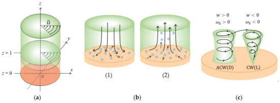
Figure 3.
Chiral vortex formation under a rotating fluid layer. (a) Two layers model of the chiral nucleation. (b) Two kinds of vortices. (1) Downward vortex; (2) upward vortex. (c) Continuity of vortex motion and fluid flow. , , and stand for the non-dimensional coordinates normalized by the average size of vortices.
Adopting the notation of a right-handed system, we can define anticlockwise (ACW) and clockwise (CW) rotations in a bird’s eye view as positive and negative, respectively. In the lower layer, microscopic vortices are first activated by the vertical magnetic field. As will be discussed precisely, they are composed of numerous pairs of vortices with upward and downward flows, respectively. As shown in Figure 3b, a downward vortex blows away ionic vacancies by the downward flow at the bottom, locally exposing rigid surfaces with friction. It works as a kind of pin to fix the vortex at a given point. In view of a nesting-boxes structure, the locally exposed surfaces correspond to the bottoms of the smaller-level vortices with downward flows. Since the positions are kept constant, at the bottoms of the vortices, chiral nuclei develop with time (1). An upward vortex pumps up ionic vacancies with the upward flow from the electrode surface so that its bottom is covered with ionic vacancies, forming a free surface without friction. The bottom of an upward vortex, differently from a downward vortex, rotates on the free surface, providing a flat surface without chiral nuclei. Though such a self-rotation, due to the pinning effect of the downward vortices, the upward vortex also does not move with the VMHDF, keeping the position constant (2). That is, downward vortices work as pins to stop the lower layer vortices to revolve with the upper layer, whereas the upward vortices supply free surfaces covered with ionic vacancies. Such different types of surfaces provide the different growth rates of vortices determining which vortices receive the precessions. At the same time, Figure 3c shows an important fact that, from the continuity of the vortex motion, a pair of adjoining upward and downward vortices must rotate in opposite directions. Then, as will be shown in Figure 4a, the individual vortex motions in the lower layer are transferred to the upper layer, where the newly induced vortices rotate with the upper layer, receiving the precessions. The precessional motions of the vortices in the upper layer are donated to the vortices in the lower layer.
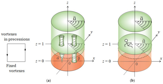
Figure 4.
Two-layer model of chiral nucleation. (a) A feedback cycle between the vortices in the lower and upper layers. (b) An observer on a frame of reference rotating with the upper layer. , , and stand for the non-dimensional coordinates normalized by the average size of vortices.
2.1. Vortex Motions in the Stationary Lower Layer
First, we consider explicitly the inertial frame with a static magnetic field. Because the sizes of fluctuations are much smaller than the belonging area of the electrode, a Cartesian coordinate system is taken for the special area, i.e., the electrode surface for the 2D nucleation or the surface of a 2D nucleus for the 3D nucleation.
Then, we consider an incompressible fluid at a uniform temperature, so the basic equations are given in the following (Appendix B) [65]. The momentum equation is in tensor notation,
where . is the velocity component of vortices (), and the Cartesian coordinate is expressed by and are the kinematic viscosity and the density, respectively. P is the pressure, and is the magnetic permeability. is the magnetic flux density, and is the i-component of .
In view of an incompressible fluid, the continuity equation is obtained.
In an electrolytic solution, the electricity is carried by diffusion as well as conductivity of ionic species, so that the current density will be given by
where is the electric field, and is the electrical conductivity defined by
where is the charge number, including the sign, is the mobility, is the Faraday’s constant, is the concentration of ionic species i, and is the diffusion coefficient. The equation of magnetic flux density is simply written in the tensor notation as follows.
where is the resistivity defined by
and implies .
As the reaction proceeds, the magnetic flux density first fluctuates, expressed by (Appendix C)
where is the external magnetic flux density in the absence of the reaction and is the fluctuation by the reaction. The fluctuation of the Lorentz force is written as
The concentration of the metallic ion is expressed by
where and are the concentration in the absence of fluctuation and the concentration fluctuation, respectively.
The mass transfer equation of the fluctuation is written as
where is the -component of the velocity, is the average concentration gradient in the diffusion layer.
where implies the concentration difference between the bulk and the surface and is the average thickness of a diffusion layer.
The i-component of the current density fluctuation is in tensor notation.
where denotes the transposition of the tensor. Then, the i-component of the vorticity is given by
Then, we shall restrict our discussion of this problem to the case where magnetic flux density is imposed vertically to the electrode.
where is the vertical magnetic flux density with the sign. Therefore, we obtain the fluctuation equations.
2.2. Amplitude Equations of the Fluctuations in the Lower Layer
For the fluctuations including vortex motions, we assume the following 2D plane waves (Appendix D).
Substituting Equations (D1a)–(D1e) into Equations (C7) and (C20a)–(C20e), we obtain the amplitude equations. Since the fluctuations are at quasi-steady states, neglecting the time-differential terms, we finally have
Substituting Equation (D3b) into Equation (D3c), and using Equation (B14) in Appendix B, we have
Then, the substitution of Equation (D3a) into Equation (D3d) leads to
where the magneto-induction coefficient is defined by
Here, we introduce a representative length . Then, let be the wavenumber in a non-dimensional unit. We shall, however, let , , and stand for the non-dimensional coordinates normalized by , so that the following parameter and operator are changed as follows.
2.3. Vortex Motions Induced in the Rotating Upper Layer
The upper layer is a reservoir of the vortices activated in the lower layer. In the lower layer, the activated vortices, due to the pinning effect of the downward vortices, keep their positions constant. On the contrary, in the upper layer, due to the rotation of the upper layer, the vortices induced by the vortices in the lower layer change their positions, revolving with the upper layer. At the same time, they start precessional motions. Then, through the upper boundary between the upper and lower layers, the motions conferred by the upper-layer rotation are transferred to the lower-layer vortices. All these processes, as shown in Figure 4a, form a positive feedback cycle.
Due to the low electric conductivity of an electrolytic solution, the electromagnetic induction by the upper layer vortices is neglected, so for simplicity, we only think of the effects of Coriolis force and centrifugal force. As shown in Figure 4b, let us consider an incompressible fluid of the upper layer rotating with an angular velocity In a frame of reference rotating with the same angular velocity, an observer at rest recognizes two kinds of acceleration (Appendix E) [65], i.e.,
where denotes the vector of the angular velocity, is the vector of the velocity, and is the position vector.
The term represents the Coriolis acceleration and the term is the centrifugal force. The velocity is expressed by the main flow component of the rotation and the activated vortex flow , i.e.,
However, since the observer is rotating with the upper layer, it follows that
The acceleration in Equation (E1) is fluctuated, expressed in the tensor notation.
where the first and second terms on the right-hand side of Equation (E5) denote the contributions of the Coriolis and centrifugal forces, respectively, where the second term is equal to zero without fluctuation.
Considering that a vector of rotation is an axial vector with -axis, we can write down the following notation,
where is the angular velocity of the upper layer. Therefore, we obtain the equations of the -components of the vorticity and velocity for the vortices.
and
Substituting Equations (D1a) and (D1b) in Appendix D into Equations (E15) and (E16), and considering that the fluctuations are in a quasi-steady state, we disregard the time differential terms. Then, let be the wavenumber in the non-dimensional. We shall, however, let , , and stand the coordinates in the new unit of length . As a result, Equations (E15) and (E16) are changed to
and
where is defined by the new coordinate as , and the rotation coefficient is expressed by
At the boundary between the upper and lower layers, the lower-layer vortices will receive the precessional motions from the upper-layer vortices shown in Equations (E20a) and (E20b).
2.4. Boundary Conditions
2.4.1. Hydrodynamic Conditions
The fluid in the lower layer is confined between the electrode and the upper layer. For convenience, the positions of the lower and upper boundaries are defined as 0 and 1 by the scale of length , which is equalized to the autocorrelation distance of the fluctuation, i.e., the average size of the vortices.
Then, regardless of the nature of the boundary surface on the electrode, rigid or free, we must require
We shall distinguish two kinds of boundary surfaces—the rigid surface on which no slip occurs and the free surface on which no tangential stress acts.
- (a)
- For the rigid surfaces:
Consider first the rigid surface. The condition that no slip occurs on the surface implies that , as well as the horizontal components of the velocity, and vanish, i.e., Since such a condition must be satisfied for all coordinates and on the surface, it follows from the continuity equation, Equation (B8) more explicitly, that
The condition of the normal component of the vorticity can also be deduced. More explicitly, is expressed by , so that we have
Substituting Equations (D1a) and (D1b) into Equations (2), (3) and (4), we obtain the following amplitude conditions.
- (b)
- For the free surfaces:
The conditions on the free surface are that the stress tensors are zero, i.e.,
Since the isotropic term has no transverse component, the condition Equation (6) is equivalent to the vanishing of the components and of the viscous stress tensor.
and
where implies the viscosity of the solution. As vanishes for all - and -coordinates on the boundary surface, it follows from Equations (6), (7a) and (7b) that
Substitution of Equation (7c) into the equation of continuity differentiated with respect to , leads to
Then, substituting Equation (7c) into the equation of (Equation (C10)) differentiated by , , we have
From Equations (2), (8) and (9), we have
- (c)
- For the upper boundary between the lower and upper layers:
Since the upper and lower layers are hydrodynamically connected, w and do not vanish at the upper boundary, and there is no slip there. The boundary conditions at the upper boundary are given by Equations (E20a) and (E20b). In the lower layer, Equations (D6a) and (D6b) are fulfilled. Therefore, from Equation (E20a), we have the upper boundary condition,
and inserting Equation (D6b) into Equation (E20b), we obtain the simpler condition.
2.4.2. Mass Transfer Conditions
In addition to the hydrodynamic conditions, we can also write down the mass transfer conditions. From Fick’s first law, we obtain the following relationship between the current density fluctuation and the concentration fluctuation .
where and are the charge number of the metallic ion and the diffusion coefficient, respectively. At the upper boundary, it is assumed that the concentration fluctuation vanishes.
As a result, using the amplitudes and , we have
and
The conditions of Equations (14a) and (14b) suggest that two arbitrary constants in the solution of the concentration fluctuation are required.
2.5. Solutions of and in the Lower Layer
From Appendix I, the general equation of the amplitude of the -component of the velocity is provided by
where , and are arbitrary constants. Then, the first and second derivatives are derived as follows:
and
The vorticity in the lower layer is affected by the precessional motions in the upper layer at the upper boundary. In view of the boundary conditions in Equations (11a) and (11b) at the upper boundary, two arbitrary constants are necessary. This means that the vorticity depends only on , so that is expressed by
where and are arbitrary constants. The first and second derivatives are
and
The individual rigid and free surface components of and are determined in the following.
- (a)
- For the rigid surface vortices:
Substituting Equations (I12), (I13) and (I14a) into Equations (5a)–(5c), we obtain
Inserting Equations (15a)–(15c) in Equations (I12) and (I13), we obtain the expressions for the rigid surface vortices,
and
where the subscript ‘r’ implies the rigid surface component. denotes the vorticity coefficient of the rigid surface vortices. Using the upper boundary conditions in Equations (11a) and (11b), we will determine the velocity coefficients and of the rigid surface vortices as the functions of .
- (b)
- For the free surface vortices:
Substituting Equations (I12), (I14b) and (I15a) into Equations (10a)–(10c), we obtain
Inserting Equations (17a)–(17c) in Equations (I12) and (I13), we obtain the expressions for the free surface vortices,
and
where the subscript ‘’ implies the free surface component. denotes the vorticity coefficient of the free surface vortices. Using the upper boundary conditions in Equations (11a) and (11b), we will determine the velocity coefficients and of the free surface vortices as the functions of .
2.6. Determination of the Velocity Coefficients and
- (a)
- For the rigid and free surface vortices at the upper boundary:
At the upper boundary, we have two relationships. First, by substituting Equations (I13), (I14a) and (I15b) into Equation (11a), we have
Then, the substitution of Equations (I14b) and (I15a) into Equation (11b) leads to
- (b)
- For the rigid surface vortices in the lower layer:
Substituting Equations (15a)–(15c) into Equations (19a) and (19b), we have
and
Equations (20a) and (20b) form simultaneous equations with respect to and , so that the following solutions are derived.
where is given by
and
where is expressed by
Here, we use the following formula.
- (c)
- For the free surface vortices in the lower layer:
Substituting Equations (17a)–(17c) into Equations (19a) and (19b), we have
and
Equations (24a) and (24b) form simultaneous equations with respect to and , so that the following solutions are derived:
where is defined by
and
where is written by
2.7. The Solution of and at the Electrode Surface
As shown in Appendix J, using the solution of in Equation (I12), we solve Equation (D3e). The general expression of is given by
We also have the first derivative with respect to z
where the mass transfer coefficient is defined by
Therefore, at the electrode surface, we have
and
where denotes an arbitrary constant. Using the amplitude equations of the current density, vorticity, and mass-flux fluctuations in Equations (D3b), (D3c) and (14a), respectively, we finally obtain the following equations, removing the arbitrary constant .
and
where the magneto-viscosity coefficient is defined by
In Equations (J14) and (J16), the coefficients are undecided, so using the conditions of the rigid and free surface vortices, we determine them in the following.
- For the rigid surface vortices:
Substituting Equations (15a)–(15c) into Equations (J14) and (J16), we have
and
Then, substitution of Equations (21a), (21b), (22a) and (22b) into Equation (27b) leads to
The residual undetermined parameter, i.e., the vorticity coefficient of the rigid surface vortex in Equations (27a)–(27c) will be determined by examining the actual formulation of 2D or 3D nucleation.
- (b)
- For the free surface vortices:
Substituting Equations (17a)–(17c) into Equations (J14) and (J16), we have
and
Then, substitution of Equations (25a), (25b), (26a) and (26b) into Equation (28b) leads to
The residual undetermined parameter, i.e., the vorticity coefficient of the free surface vortex in Equations (28a)–(28c) will be determined by the actual formulation of 2D or 3D nucleation.
3. 2D Nucleation
3.1. Asymmetrical Fluctuations in 2D Nucleation Process
The 2D nucleation proceeds in an electric double layer. As shown in Figure 5, at the inner Helmholtz plane (IHP), dehydrated metallic ions receive electrons, being adsorbed as adatoms on the electrode surface [22].
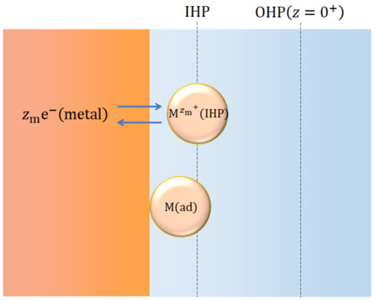
Figure 5.
The 2D nucleation in an electric double layer.
Assuming equilibrium between the metallic ions at the IHP and the adatoms at the metal surface, the electron-transfer reaction is written as
where and are the adatom and the metallic ion at the IHP, respectively, and is the free electron at the electrode.
According to Equation (29), their chemical and electrochemical potentials are related with
where implies the chemical potential of the adatom. denotes the surface deformation by 2D nucleation formed by asymmetrical fluctuations, is the electrochemical potential of the metallic ion, and is the electrochemical potential of a free electron.
At the equilibrium potential, physical quantities fluctuate toward the positive and negative sides of their equilibrium states (Figure 6a). However, when the potential is deviated from the equilibrium to the cathodic direction, the cathodic reaction proceeds, and various asymmetrical fluctuations, including 2D nucleation, develop around the electrode. As shown in Figure 6b, they one-sidedly fluctuate from their equilibrium states, i.e., whether plus or minus, their signs are kept constant. This means that in a nonequilibrium state, either side of the amplitude of an equilibrium fluctuation is cut off (phase cutting).
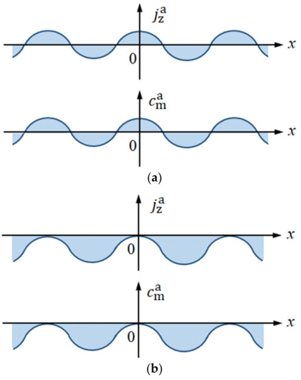
Figure 6.
Equilibrium and nonequilibrium fluctuations. (a) Equilibrium concentration fluctuation. (b) Nonequilibrium concentration fluctuation in a cathodic deposition.
Due to large mobility in light speed, the fluctuation of the electron can be neglected in steady-state, so from Equation (30), the relationship between the fluctuations is expressed by
where superscript ‘’ implies asymmetrical fluctuation. Due to the small curvature of a 2D nucleus, the chemical potential fluctuation of the adatom, which arises from the change of the surface form of the deposit can be neglected , so that we have the following condition of the electrochemical potential fluctuation of the metallic ion.
Accompanied by electrolytic current flowing, asymmetrical potential and concentration fluctuations occur. Based on Fick’s first law, at the outer Helmholtz plane (OHP), , the current density fluctuation is written by
In the presence of a large amount of supporting electrolytes, from Equation (B9), the current density fluctuation is also described by the potential fluctuation as follows:
where implies the asymmetrical fluctuation of the overpotential in the diffuse layer. From Equations (33a) and (33b), we obtain
Since both fluctuations have the same function form of , Equation (33c) supplies the equation,
At the same time, the electrochemical potential fluctuation is also represented by these fluctuations,
where and are the overpotential fluctuations at the inner Helmholtz plane (IHP) and at the surface of a 2D nucleus in the diffuse layer, respectively. is the surface concentration outside the double layer, is the universal gas constant ( J K−1 mol−1), is the absolute temperature (K), and is the Faraday constant ( C mol−1).
By expanding with respect to the -coordinate at the flat OHP without the 2D nuclei, the potential fluctuation at the surface of a 2D nucleus is expressed by
is the gradient of the electrostatic overpotential in the diffuse layer defined by [22]
where is the electrostatic overpotential at a flat OHP without 2D nuclei measured from the outer boundary of the diffuse layer , and is the Debye length equalized to the average diffuse layer thickness.
where is the dielectric constant of water (6.95, 25 °C), is the charge number including sign, and is the bulk concentration of ionic species j except for the bulk metallic-ion concentration (mol m−3).
The concentration fluctuation in the diffuse layer is correspondingly expressed by
where is the average concentration gradient of the metallic ion in the diffuse layer [66], which is defined by
Equations (35b) and (36b) have the relationship,
Here, the overpotential fluctuation of the Helmholtz layer is induced by the fluctuation , which is depicted by the differential potential coefficient in Equation (A1) in Appendix A.
Substituting for from Equation (38) in Equation (34), then inserting Equations (36a) and (37) into the resulting equation, we obtain
Under the limiting diffusion condition, the surface concentration is sufficiently small in limiting diffusion, so that substituting for from Equation (33d) in Equation (39a), we can derive the following condition:
Using Equations (35b) and (39b), we obtain the electrochemical potential fluctuation at the top of a nucleus, which is represented by
Applying the electrochemical condition Equation (32) to Equation (39c), we have the relationship between and .
Due to small wavenumbers of the fluctuations arising from large 2D nuclei, a higher order of smallness, such as surface energy, can be disregarded [22]. Considering that the surface deformation results from the mass transfer of metallic ions, we obtain
where represents the molar volume of the deposited metal (m3 mol−1).
Here, in the scale of unit length of the asymmetrical fluctuations, the coordinate of the electrode surface is equalized to the coordinate of the OHP , so that at the OHP is regarded as at the electrode surface. Therefore, the substitution of Equation (40) into Equation (41) leads to
Equation (42) is transformed in terms of Fourier transform regarding - and -coordinates, i.e.,
where implies , and is the adsorption coefficient.
3.2. Characteristic Equations of the Vorticity Coefficients and
As will be shown below, the characteristic equations of the micro-MHD flows on the rigid and free surfaces (i.e., rigid and free surface vortices) are derived as the equations of the vorticity coefficients and , which are solved under the condition,
Here, for 2D nucleation, corresponds to the angular velocity of a VMHDF. As shown in the preceding papers [5,6], according to Equation (44), the sign of , i.e., the rotational direction of a VMHDF is determined by the sign of , i.e., the direction of the magnetic field.
- (a)
- For the rigid surface vortices:
Substituting from Equation (27a) and from Equation (27c) in Equation (43a), we obtain the following characteristic equation of the vorticity coefficient for the rigid surface vortices in 2D nucleation.
where implies the amplitude factor function of the rigid surface vortices in 2D nucleation.
where, since Equation (44) is always fulfilled, has no singular point and takes positive values.
As shown in Appendix G, the coefficients , , , and are redefined in accordance with 2D nucleation as follows.
- (b)
- For the free surface vortices:
Substituting from Equation (28a) and from Equation (28c) in Equation (43a), we obtain the following characteristic equation of the vorticity coefficient for the free surface vortices:
where implies the amplitude factor function of the free surface vortices in 2D nucleation.
and
where, since Equation (44) is always fulfilled, has no singular point and takes positive values. The characteristic equation, Equation (47a), can always be solved, i.e.,
where means the amplitude factor of the free surface vortices.
From Equations (46a) and (48a), we can determine whether the activated vortices are stable or unstable. If the amplitude factors and are negative for all wavenumbers, the fluctuations, as well as the vortices, are stable, stochastically repeating activation and extinction. On the contrary, when they are positive for some of the wavenumbers, the corresponding fluctuation components once activated become unstable, deterministically developing with time.
In Figure 7, the representative function forms of and against the non-dimensional wavenumber are exhibited. As discussed above, they are always positive for , and is larger than . As will be discussed later, when the adsorption coefficient is negative, i.e., in non-specific adsorption of ions, the free surface vortices receive the precessions since the free surface vortices grow faster than the rigid surface vortices. On the other hand, in the case of specific adsorption, due to positive , the rigid surface vortices dwindle more slowly than the free surface ones, so that the rigid surface vortices will receive the precessions.
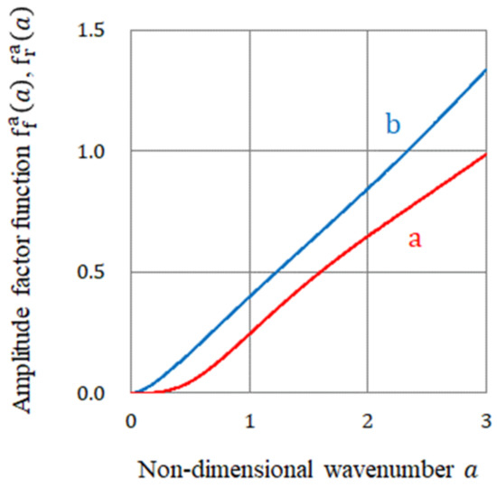
Figure 7.
Amplitude factor functions vs. non-dimensional wavenumber . a, of the fluctuations on the rigid surfaces. b, of the fluctuations on the free surfaces.
However, under some other conditions, if the difference of both functions became smaller, slight changes in the initial situation would easily lead to the inversion of the vortices receiving the precessions, i.e., breaking of chiral symmetry.
3.3. Nucleation by the Rigid and Free Surface Vortices
To calculate the nucleation with the rotations of the rigid and free surface vortices, we must solve the self-organization problem concerning two independent fluctuation components at once. This means that we must treat a two-components vector so that it is convenient to embed the amplitudes of both components in a single complex number.
We first suppose a horizontal wavenumber plane divided by 2D grids, where in the vertical -direction, a solution phase and an electrode phase are defined. Then, considering a stochastic process in multi-nucleation of electrodeposition, we introduce a unit random complex number in the following: In the vertical -direction within the autocorrelation distance of the fluctuation , i.e., in the lower layer , the same random numbers are used, so that we define the following 2D random number.
where is a uniform random number between 0 and , which is assigned to all grid points defined on the plane. As a result, the actual values of and in Equations (46a) and (48a) are expressed by
Though the same random number is used, since the two components on the rigid and free surfaces are normal to each other, they are defined independently.
According to the discussion in Appendix F, the initial concentration fluctuation is assumed to have the following Gaussian-type power spectrum.
where is defined. Substituting Equations (G7a) and (50a) into Equation (46a), we have the exact expression of .
where the power spectrum component plays a low-pass filter concerning the wavenumber for the fluctuations. The constant part of the vorticity coefficient of the rigid surface vortex in 2D nucleation is given by
where and are - and -lengths of the electrode, respectively, and is the initial ratio of the rigid surface component to the total concentration fluctuation. As discussed initially, the rigid and free surface components, as well as the vortices, distribute equally over the electrode, so that equal to that of the free surface component is assumed. For cathodic deposition, the concentration difference is fulfilled, so that is derived. Substitution of Equations (G10a) and (50b) into Equation (48a) leads to the explicit equation of the vorticity coefficient of the free surface vortices.
The constant part of the vorticity coefficient of the free surface vortex in 2D nucleation is given by
where is assumed as the initial ratio of the free surface component to the total concentration fluctuation and for deposition, is obtained. Equations (51a) and (51b) show that the vorticity coefficients are also restricted by the initial spectrum component .
After assigning the random numbers at all grid points in the solution phase and considering the stochastic effect of Equations (50a) and (50b), the amplitude of the gradients of the concentration fluctuations in Equations (G8b) and (G11b) is rewritten as
and
and must independently distribute over the electrode surface without any contradiction, which mathematically implies that they are orthogonal normal packed.
To self-consistently calculate their self-organization processes, a complex Fourier transform is used, e.g., the rigid and free surface components are embedded as the real and imaginary parts in the forms of odd and even functions, such as sine and cosine functions concerning the wavenumber, respectively. Generally, the odd and even functions are normal to each other, whose symmetries are preserved in the transform.
In accordance with the above discussion, to embed the odd and even functions into a complex space, the following operator is introduced.
or
where ‘(even)’ and ‘(odd)’ imply the even and odd functions embedded in the real and imaginary parts, and vice versa. Then, the allotment of random numbers to the 2D grids allows us to introduce random phases to the odd and even functions.
As a result, the complex amplitude of the concentration gradient function with random phases is expressed in the following.
The is transformed to the complex concentration gradient by the complex Fourier inversion, i.e.,
where it should be noted that the coordinates and are defined as non-dimensional. The Fourier transformation makes only periodic components transformed. After obtaining the result, to reproduce the actual form of the asymmetrical fluctuation, some average values regarding - and -coordinates must often be added to it. The complex amplitudes of the rigid and free surface components are transformed to the concentration gradient in a complex space in keeping their symmetries, i.e.,
where and are the rigid and free surface concentration fluctuations, respectively. The rigid and free surface components are transformed as even and odd functions with random phases of the - and -coordinates, respectively. As shown in Figure 6b, nonequilibrium fluctuations have either sign of positive or negative. For cathodic deposition, the concentration and concentration gradient fluctuations take negative and positive values, respectively. To derive the negative current density, with the root mean square (rms) values of the fluctuations, we must cut off the extra negative portions of the concentration gradient fluctuations. From Rayleigh’s theorem, the mean square value of the concentration gradient fluctuation is equalized to the mean square value of its amplitude.
For the rigid or free surface component, it follows that
where X and Y imply the - and -lengths of the electrode. From Equation (56a), the root mean square (rms) value of the concentration gradient can be calculated by the rms value of the amplitude as follows.
Therefore, by adding the root mean square value, the “phase cutting” is completed, i.e., the concentration gradient fluctuations are redefined.
The concentration gradient distributed over the electrode surface is completely reproduced by the linear combination of the rigid and free surface components of the even and odd functions with respect to - and -coordinates.
Finally, the current densities on the rigid and free surfaces are derived from Fick’s first law in the following.
and
The total current density is thus expressed by
As a result, the surface morphology of the 2D nuclei is effectively calculated by the surface height fluctuation.
where implies the molar volume of the deposit metal. Based on Equations (59a) and (59b), the surface morphology of the 2D nuclei can be divided into the rigid and free surface components, i.e.,
3.4. The Rotational Directions of the Micro-MHD Flows on the Rigid and Free Surfaces
As discussed initially, we can determine the characteristics of the rigid and free surface vortices by the signs of the -components of the velocity and vorticity fluctuations. Namely, the rigid and free surface vortices correspond to the vortices with downward and upward flows, which are expressed by the negative and positive values of the -components of the velocity fluctuation, respectively. In addition, the CW and ACW rotations are provided by negative and positive values of the -component of the vorticity.
As shown in Appendix H and Appendix K, the - and -components of the velocity are calculated by the -components of the velocity and vorticity.
- (a)
- For the rigid surfaces:
Using Equations (21a) and (22a), we redefine Equation (16a) as
Then, inserting Equation (51a) into Equation (60), we obtain
Replacing in Equation (16b) with in Equation (51a), we have
where Equations (21b) and (22b) supply the following expressions.
and
- (b)
- For the free surfaces:
Using Equations (25a) and (26a), we redefine Equation (18a) as
Inserting Equation (51b) into Equation (63), we obtain
Inserting Equation (51b) into Equation (18b), we have
where Equations (25b) and (26b) supply the expressions of and .
and
Then, the rigid and free surface components are embedded into real and imaginary parts of a complex amplitude in the forms of even and odd functions regarding the wavenumber.
and
In accordance with the above discussion of the 2D nucleation, the actual -components of the velocity and vorticity fluctuations are calculated by the following complex Fourier inversions, where the rigid and free surface components are embedded as real and imaginary parts in the forms of even and odd functions regarding - and -coordinates, respectively.
and
As discussed in Equations (55a) and (55b), the Fourier transform makes the transformation of the periodic components, so that the actual forms are reproduced by adding the average components to them. As mentioned above, the vortices are classified by four characters; the rigid and free surface components correspond to the downward flow and the upward flow , respectively. On the other hand, the rotational directions are determined by the precessions from the upper layer. CW and ACW rotations in bird’s-eye view correspond to the negative vorticity and the positive vorticity for or f, respectively. Therefore, in accordance with Equation (56c), we redefine the velocities and vorticities.
For the rigid surface vortices, we have
and
For the free surface vortices, we have
and
where and () imply the rms values of and , which are expressed by
and
Actual distributions of the velocity and vorticity are expressed by the linear combinations of rigid and free components, respectively.
and
As mentioned above, the pair of vortices are composed of the vortices with opposite -components of velocities and vorticities, and downward and upward -components of the velocity correspond to rigid and free surface vortices. Since a pair of vortices with upward and downward flows have opposite rotations, as shown in Figure 8, the vortices are simply classified into two sets, where the distributions of the phase-cut quantities in -direction are schematically exhibited.
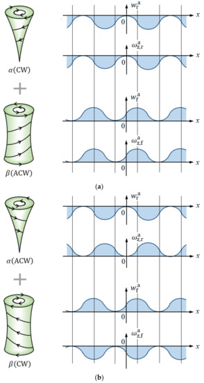
Figure 8.
Two sets of the micro-MHD vortex pair formed on the rigid and free surfaces. (a) CW-ACW vortex pair. (b) ACW-CW vortex pair. , rigid surface vortex; , free surface vortex; , -velocity component of the rigid surface vortex; , -vorticity component of the rigid surface vortex; , -velocity component of the free surface vortex; , -vorticity component of the free surface vortex.
As shown in Figure 9, the formation processes of chiral 2D and 3D nuclei plus chiral screw dislocation constitute nesting boxes, i.e., chiral 2D nuclei develop on an electrode, chiral 3D nuclei grow on a chiral 2D nucleus, and chiral screw dislocations are created on a chiral 3D nucleus. As discussed initially, for chirality to emerge, two types of vortices are necessary. One of them (i.e., the rigid surface vortex) directly contributes to the chiral nucleation, where the rigid surfaces under a vortex of the micro-MHD flow are formed by locally exposed rigid surfaces, such as a bee’s nest. Each local rigid surface corresponds to the bottom of a smaller rigid surface vortex, yielding a chiral nucleus of the next generation. On the other hand, on the free surfaces covered with ionic vacancies, due to the moving solution of a vortex at the electrode surface, such microstructures of 3D nuclei are not created.
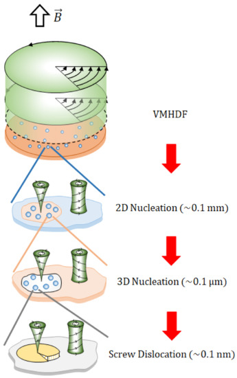
Figure 9.
Nesting-boxes structure of chiral 2D and 3D nucleation plus chiral screw dislocation.
4. Results and Discussion
4.1. Micro-Mystery Circles Formed by the Non-Specific Adsorption of Ions
Figure 10 exhibits the copper electrode surfaces deposited under a VMHDF. Through the deposition, characteristic concave round patterns with diameters of the order of 100 , called micro-mystery circles, were observed (Figure 10a). However, after encircling the VMHDE with a sheath to stop the rotation of the VMHDF, such patterns disappear on the deposit surface (Figure 10b). Since these experimental results do not directly indicate the chirality of the 2D nuclei, in the following, based on the theoretical foundation discussed above, we calculate the morphological pattern of the micro-mystery circle and examine whether such a concave pattern is theoretically reproduced or not.
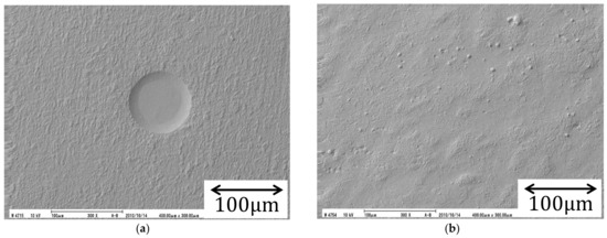
Figure 10.
SEM images of the surface morphologies of copper electrodeposition under vertical magnetic fields. (a) A micro-mystery circle formed by a VMHDF. (b) Disappearance of the micro-mystery circle by the blocking of VMHDF with a sheath. Though the applied magnetic flux density is different, i.e., (a) 3 T and (b) 1 T, the other conditions are the same. Deposition time is s. A mol m−3 CuSO4 + mol m−3 H2SO4 solution was used at room temperature.
In the preceding paper [21], it has been clarified that the MHD flow patterns formed on the copper deposit surface are reproduced after multiple nucleation. In accordance with the procedure shown in Equations (49)–(59c), we calculated the copper deposit surfaces after repeating the one hundred-times nucleation under a VMHDF: Assigning random numbers to the grid points of a defined electrode surface at the beginning of each nucleation, 2D nuclei start to develop with time, expanding two-dimensionally, so that at their borders, some disorders take place. In actual 2D nucleation, such disorders would be self-consistently reformed. However, in this theory, because the treatment of such boundary disorders is not considered, as shown in Figure 11, the disorders of the boundaries remain as they are. In the calculated images, the concave circular patterns of the same order of magnitude as the SEM image appear on the deposit surface. In the present case of nonspecific adsorption of ions, the nucleus on the rigid surface grows more slowly than the nucleus on the free surface, so we can expect that the concave part is mainly composed of the rigid surfaces of 2D nuclei involving chiral 3D nuclei. We can also suppose that chiral screw dislocations would be created on the 3D nuclei. Namely, in quite high probability, it is expected that the chiral activity exists on the concave part.
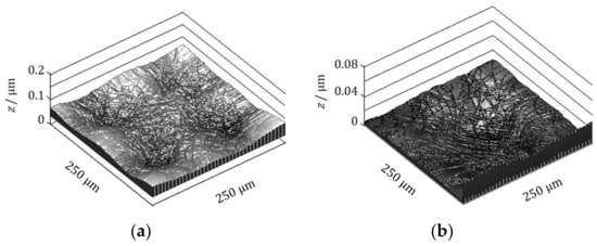
Figure 11.
Theoretical calculation of micro-mystery circles after multiple 2D nucleation. (a) The case of four circles. (b) The case of a single circle. Calculation data are as follows: , 62.8 s−1, m2 s−1, m, mol m−3. Supporting electrolyte, 500 mol m−3; applied overpotential, −0.4 V; nucleation period, 1.0 s; nucleation number, 100.
As discussed initially, due to the conservation of angular momentums of the vortices activated from a stationary state, vortices with ACW and CW rotations are equally evolved, so that half of the nuclei randomly created in each generation would be chiral ones formed on the rigid surfaces. In view of the nesting-boxes structure of the chiral nucleation shown in Figure 9, the probability that the chiral screw dislocations emerge from all active points is obtained by the product of the probability of each generation.
Equation (72) is derived from the three-generation model of chiral nucleation under the initial condition that rigid surface and free surface vortices are equally distributed over the electrode. This is a strong restriction for all the vortices in the three generations.
The created screw dislocations act as single active points for enantiomeric reagents. Figure 12 schematically exhibits D-active and L-active surfaces of a nucleus, i.e., the surfaces are uniformly covered with single and achiral active points. A single active point is active for either D- and L-reagents and inactive for the other one, whereas an achiral active point is active for both D- and L-reagents. Owing to the uniform distribution, we can calculate the reaction current of the electrode by the ratios of the single active points and achiral active points, i.e., and , respectively.
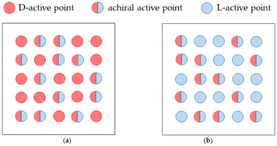
Figure 12.
D-active and L-active surfaces of a nucleus. (a) D-active surface. (b) L-active surface. Red circle, D-active point; blue circle, L-active point; semicircles of red and blue, achiral active point.
Because an achiral active point is composed of both D- and L-active portions, the probability for an enantiomeric reagent to react at the active point is equal to 1/2. Therefore, we can assume that the activity of an achiral active point is half of a single active point. In view of twice larger activity of a single active point, for the electrode active for either D- or L-reagents, the total current is written by
where implies the total current of the electrode covered with only achiral active points.
On the other hand, the single active point of the electrode is inactive for the other reagent, so that for the reagent, the current component of the single active point becomes zero, and the total current is equal to the current of the achiral active points.
Using Equations (73a) and (73b), we can calculate the absolute value of the enantiomeric excess (ee) ratio defined by Mogi, i.e.,
where the ee ratio itself is defined as positive for L-activity and negative for D-activity. The absolute value of the ee ratio is equal to the probability that the chiral screw dislocations emerge from all the active points. Since corresponds to an ideal limiting case, we can conclude that the absolute value of the ee ratio cannot exceed 0.125.
Equation (74) is supported by the experimental data of Mogi’s reports [9,10,11,12,13,14,15,16,17,18]. Namely, the three-generation model is experimentally validated. An ee ratio of is declared as the ideal limiting value obtained by the present method, which results from the fact that the evolution probability of the rigid surface vortex is equal to that of the free surface vortex.
4.2. Inversion of Chirality by the Specific Adsorption of Chloride Ions
As mentioned above, the magnetic field, current, and Lorentz force consist of a right-handed system, so that according to the law of a right-handed system, Equation (44) is always fulfilled. As a result, under a parallel magnetic field or an antiparallel magnetic field in a bird’s-eye view, the upper layer, i.e., the VMHDF rotates in a clockwise or an anticlockwise direction, respectively. Then, the vortices in the lower layer receive the precessions from the upper layer via the vortices in the upper layer. As shown in Figure 2C, due to the continuity of the vortex motion, two adjoining vortices form a pair of vortices with reverse rotations as well as downward and upward flows, so that a rigid surface vortex appears with a free surface vortex. If either of them starts a precessional motion, the other must subordinately rotate in the opposite direction. Then, the next problem is which the vortex receives the precession, rigid or free surface. There are two cases, i.e., one is an unstable case where the vortices develop with time and the other is a stable case where the vortices, once activated, dwindle with time.
As discussed in Equations (46b) and (48b), in accordance with the signs of the amplitude factors and , the micro-MHD vortices will develop or decay with time. As shown in Figure 7, the amplitude factor functions and in Equations (45b) and (47b), always take positive values for all wavenumbers, so that from Equations (46b) and (48b), the signs of (i.e., ) and (i.e., ) determined by the adsorption coefficient shown in Equation (43b), whose sign depends on the sign of the product of the differential potential coefficient and the overpotential at the OHP(). As discussed in Appendix A, as for ionic adsorption, the following conditions concerning unstable and stable growths of the fluctuations are derived.
In accordance with Appendix A, the present case shown in Equation (76a) certainly corresponds to the non-specific adsorption, whereas Equations (76b) and (76c) indicate the strong specific adsorption of chloride ions. Since the chemical bonding force of a chloride ion is stronger than the repulsive electrostatic force, it can adsorb on the copper cathodic surface. For a mol m−3 H2SO4 supporting electrolyte solution, from Equation (35c), we obtain the Debye length λ m. Using F m−2 as well as Equation (75), we have the differential potential coefficients as follows:
In view of cathodic polarization of the diffuse layer , Equation (77a) corresponds to the unstable condition Equation (A9a), whereas Equations (77b) and (77c) derive the stable condition Equation (A9b).
The differential potential coefficients in the case of the specific adsorption of chloride ions in Equations (77b) and (77c) are smaller than . These results mean that the chloride ions induce strong specific adsorption. From the discussion in Appendix A, for the non-specific and strong specific adsorptions in the cathodic deposition, the overpotentials of the diffuse layers take negative values. Assuming V, we can calculate the amplitude factors and in Equations (46b) and (48b).
As a result, in the case of the non-specific adsorptions of simple ions at the electrode surface, as shown in Figure 13a, the amplitude factors and take positive values for all wave numbers , so that the asymmetrical fluctuations, including the vortices of micro-MHD flows, become unstable, i.e., activated vortices deterministically develop with time. Due to the larger positive amplitude factor, the free surface vortices grow faster than the rigid surface ones. The precessions by the VMHDF therefore transfer to the free surface vortices, so that the rigid surface vortices creating chiral 2D nuclei rotate in the opposite direction of the VMHDF rotation, yielding 2D nuclei with opposite chirality. In unstable 3D nucleation, we can also expect that the free surface vortices on a rigid surface of a 2D nucleus are given the priority in precession. This time, due to the opposite rotational direction, the rigid surfaces of 3D nuclei and the nano-vortices will obtain the same chirality as the VMHDF. If the same process were repeated in the third generation, the screw dislocations formed on a rigid surface of 3D nucleus would obtain the opposite chirality. This means that the electrode gains the opposite chiral activity as the rotations of the VMHDF.
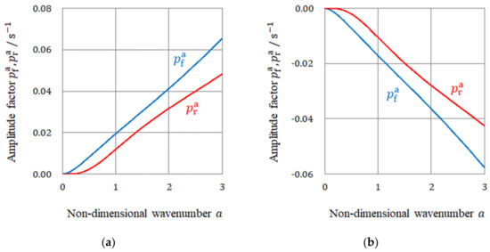
Figure 13.
Amplitude factors and for non-specific and specific adsorptions. (a) The case of non-specific adsorption. (b) The case of specific adsorption.
For the specific adsorption of chloride ions, as shown in Figure 13b, and become negative for all wavenumbers, so that the fluctuations are kept stable, i.e., an initially activated vortex dwindles to nothing with time. Such activation and extinction are stochastically repeated regarding time and location. In this case, due to the smaller negative amplitude factor, the rigid surface vortices decay more slowly than the free surface ones receiving the precessions. Therefore, in this case, 2D nuclei with the same chirality as the VMHDF rotation emerge under the rigid surface vortices. However, since 3D nuclei and screw dislocations do not grow in an electric double layer, but in a diffusion layer, their unstable free surface vortices will be again given priority in precession, so that the chirality in the first generation would be transferred to the third generation as it stands. This means that by adding a chloride additive, the electrode gains the same chiral activity as the VMHDF rotation.
As for 2D chiral nucleation, in the absence of specific adsorption of ions, it is concluded that under an upward antiparallel () or a downward parallel () magnetic field, clockwise (CW) or anticlockwise (ACW) rotations occur in the rigid surface vortices, respectively. That is, such a relationship is expressed by
where implies the representative angular velocity of the rigid surface vortices. This symmetry of rotation is consistent with the odd symmetry of chiral activity of the copper deposit surfaces.
On the other hand, for the specific adsorption, such as chloride adsorption, the amplitude factors become negative. As mentioned above, in the stable case, the rigid surface vortices rotate in the same direction as a VMHDF. Namely, in the presence of specific adsorption of ions, we can say that the rotational directions of the vortices creating chiral nuclei are reversed, i.e., upward antiparallel () and downward parallel () magnetic fields induce anticlockwise (ACW) and clockwise (CW) rotations of the rigid surface vortices, respectively, i.e.,
That is, the rotations of the rigid surface vortices of the micro-MHD flow are reversed. In this model, the chirality of the rigid surface vortices changes but the symmetry breakdown does not occur.
However, the obtained amplification factors and are not so large that both kinds of vortices would easily fluctuate between both rotational directions, giving rise to the symmetry breaking.
5. Materials and Methods
The experiment was carried out in copper electrodeposition in a 300 mol m−3 CuSO4 + 500 mol m−3 H2SO4 solution. The experimental apparatus was represented elsewhere [6]. Water was prepared by a pure water production system (MERCK KGAA, Darmstadt, Germany). The CuSO4 and H2SO4 were analytical grades (FUJIFILM Wako Pure Chemical Corporation, Osaka, Japan). The VMHDE was made of a copper disk of 8 mm diameter (oxygen-free copper, 99.99% purity, The Nilaco Corporation, Tokyo, Japan) equipped with a 5 mm-wide fringe of PTFE resin (Flonchemical Co. Ltd., Osaka, Japan). To prevent natural convection, it was set in a downward direction. The counter electrode (oxygen-free copper, 99.99% purity, The Nilaco Corporation, Tokyo, Japan) was a copper plate, 25 mm in diameter, which was placed 30 mm from the VMHDE. A copper rod (1 mm diameter) was used as a reference electrode (oxygen-free copper, 99.99% purity, The Nilaco Corporation, Tokyo, Japan). To stop the VMHDF, a sheath with an 18 mm inner diameter and an 18 mm height was attached to the electrode. By using the limiting diffusion current at an overpotential of −400 mV under a given vertical magnetic field, the experiment was performed. The whole electrode system was settled at the place of a uniform magnetic field selected in the bore space of a 10T-cryocooled superconducting magnet (HF-10-100VH, Sumitomo Heavy Industries Ltd., Tokyo, Japan). The deposited electrode surfaces were observed by a surface roughness analysis 3D scanning electron microscope (ERA-8800, ELIONIX Inc., Tokyo, Japan).
6. Conclusions
The 2D chiral nuclei are formed under the rigid surface vortices, whose chirality arises from the precessions by the VMHDF. The chiral screw dislocations grow on a chiral 3D nucleus, which in turn develops on a chiral 2D nucleus. Based on these results, the initial five questions are answered as follows.
- 1.
- Chiral screw dislocations under a VMHDF arise from the three generations of chiral nuclei, which constitute nesting boxes. Namely, chiral 2D nuclei are formed by the chiral micro-MHD vortices with rigid surfaces. Then, chiral 3D nuclei are created by the chiral nano-MHD vortices with rigid surfaces on a chiral 2D nucleus. Finally, chiral screw dislocations grow by chiral ultra-micro MHD vortices with rigid surfaces on a chiral 3D nucleus. Such a structure was validated by the fact that the observed enantiomeric excess (ee) ratios are always smaller than .
- 2.
- The chiral nucleation system is composed of a rotating upper layer and a stationary lower layer so that vortices in the lower layer can receive the precessions from the upper layer and raise chiral nuclei at fixed places.
- 3.
- For chirality to emerge, two types of vortices are necessary, having rigid surfaces with friction and free surfaces covered with ionic vacancies. Due to the rigid surface with friction, the rigid surface vortices not only work as pins to stop the migration of the vortices in the lower layer but also create chiral nuclei at fixed positions. Which vortex receives the precession depends on whether the growth mode is unstable or stable. Free surface vortices unstably grow faster than the rigid surface vortices, whereas, under stable conditions, rigid surface vortices activated dwindle with time more slowly than free surface vortices. Therefore, when unstable, free surface vortices have the priority of precession, and in stable cases, the precessions are donated to rigid surface vortices.
- 4.
- Due to fluid and vortex continuities, a pair of adjoining vortices are composed of rigid and free surface vortices with opposite rotations. To raise nuclei fixed to a solid surface, chiral nucleation must occur only under the rigid surface vortices. Since in a CuSO4 + H2SO4 solution, simple non-specific adsorption takes place, unstable copper nucleation proceeds. As a result, the rotation of a VMHDF transfers to the free surface vortices as the precessions, so that 2D nuclei with reverse chirality are formed under rigid surface vortices in the rotation opposite to that of the VMHDF. Though this result does not directly explain the chiral activity of the electrode, we can understand the mechanism of the emergence of the opposite chirality to the VMHDF. In accordance with the three-generation model, if such a nucleation process were repeated three times, the opposite chirality would be realized.
- 5.
- When a chloride additive is added to a CuSO4 + H2SO4 solution, specific adsorption of the chloride ions takes place, leading to stable nucleation. In this case, the rotation of a VMHDF is bestowed on the rigid surface vortices as precessions. Therefore, 2D nuclei growing under the rigid surface vortices have the same chirality as that of the VMHDF. Namely, due to the stability of the specific adsorption of chloride ions, we can expect a change in the chiral activity of the electrode. However, if the differences between both amplitude factors and their values themselves were sufficiently small, the breakdown would also take place.
Author Contributions
Conceptualization, R.A.; methodology, A.S., M.M. (Makoto Miura), Y.O. and R.A.; software, R.M., M.M. (Miki Miura), and R.A.; validation, A.S., M.M. (Makoto Miura), Y.O. and R.A.; formal analysis, R.M., A.S., M.M. (Makoto Miura), Y.O., S.T. and R.A.; investigation, R.M., A.S., M.M. (Makoto Miura), Y.O. and S.T.; resources, Y.O., I.M. and R.A.; data curation, R.M. and R.A.; writing—original draft preparation, R.A.; writing—review and editing, R.M., A.S., M.M. (Makoto Miura) and Y.O.; visualization, R.M., A.S., M.M. (Makoto Miura) and Y.O.; supervision, Y.Y. and R.A.; project administration, Y.O. and R.A. All authors have read and agreed to the published version of the manuscript.
Funding
This research was partially supported by the JSPS KAKENHI Grant-in-Aid for Scientific Research (C) no. 19K05230.
Institutional Review Board Statement
Not applicable.
Informed Consent Statement
Not applicable.
Data Availability Statement
Not applicable.
Acknowledgments
This work was performed in part at the Queensland node of the Australian National Fabrication Facility, a company established under the National Collaborative Research Infrastructure Strategy, to provide nano and microfabrication facilities for Australia’s researchers. The authors thank the staff members of High Field Laboratory for Superconducting Materials of IMR, Tohoku University, for the use of the cryocooled superconducting magnet, and the Tsukuba Magnet Laboratory, National Institute for Materials Science (NIMS), for the use of superconducting magnets.
Conflicts of Interest
The authors declare no conflict of interest.
Nomenclature
| , , | Cartesian coordinates corresponding to , , (m) |
| , , | non-dimensional coordinates normalized by |
| position vector (m) | |
| d | representative length (m) |
| representative length of asymmetrical fluctuations in 2D nucleation (m) | |
| , | wavenumber components in the - and -directions (m−1) |
| wavenumber defined by (m−1) | |
| , | wavenumber components of in the - and -directions |
| non-dimensional wavenumber () | |
| autocorrelation distance of the fluctuation, i.e., the average size of the vortices (m) | |
| velocity which an observer feels (m s−1) | |
| i-component of the main flow velocity of the rotation (m s−1) | |
| velocity (m s−1) | |
| i-component of (i = 1, 2, 3) (m s−1) | |
| -component of the velocity, (m s−1) | |
| -component of the velocity, (m s−1) | |
| w | -component of the velocity, (m s−1) |
| i-component of the vorticity (s−1) | |
| -component of the vorticity (s−1) | |
| -component of stream function (m s−1) | |
| -component of stream function (m s−1) | |
| Gaussian-type power spectrum defined by Equation (F5) | |
| viscous stress tensor defined in Equation (7a) (N m−2) | |
| viscous stress tensor defined in Equation (7b) (N m−2) | |
| density of solution (kg m−3) | |
| viscosity of solution (N s m−2) | |
| kinematic viscosity (m2 s−1) | |
| kinematic viscosity of bulk solution in 2D nucleation | |
| molar volume of deposit metal (m3 mol−1) | |
| P | pressure (N m−2) |
| magnetic permeability (4π × 107 N A−2) | |
| resistivity defined by Equation (B14) | |
| dielectric constant of water (6.95 × 10⁻¹⁰ J−1 C2 m−1, 25 °C) | |
| universal gas constant (8.31 J K−1 mol−1) | |
| absolute temperature (K) | |
| Faraday constant (96,500 C mol−1) | |
| magnetic flux density (T) | |
| i-component of (T) | |
| external magnetic flux density in the absence of reactions (T) | |
| j-component of (T) | |
| -component of with sign (T) | |
| fluctuation of by reactions (T) | |
| i-component of (T) | |
| -component of (T) | |
| electric field (V m−1) | |
| current density (A m−2) | |
| i-component of the current density fluctuation (A m−2) | |
| -component of the current density fluctuation (A m−2) | |
| asymmetrical fluctuation of at the electrode (A m−2) | |
| electrical conductivity (S m−1) | |
| charge number of ionic species i including sign | |
| charge number of the metallic ion | |
| mobility of ionic species i (m2 V−1 s−1) | |
| -component of unit normal vector | |
| concentration of ionic species (mol m−3) | |
| diffusion coefficient of ionic species i (m2 s−1) | |
| diffusion coefficient of the metallic ion (m2 s−1) | |
| Lorentz force per unit volume (N m−3) | |
| i-component of (N m−3) | |
| acceleration which an observer feels in a frame of reference rotation with the same angular velocity as the upper layer (N m−3) | |
| i-component of the fluctuation of (N m−3) | |
| i-component of the fluctuation of the Lorentz force (N m−3) | |
| concentration of the metallic ion (mol m−3) | |
| concentration of the metallic ion in the absence of fluctuation (mol m−3) | |
| concentration fluctuation of the metallic ion (mol m−3) | |
| asymmetrical fluctuation of the concentration of the metallic ion (mol m−3) | |
| at OHP (mol m−3) | |
| surface concentration of the metallic ion outside the double layer (mol m−3) | |
| bulk concentration of the metallic ion (mol m−3) | |
| bulk concentration of ionic species j (mol m−3) | |
| average concentration gradient in the diffusion layer defined by Equation (C8) (mol m−4) | |
| concentration difference between the bulk and the surface (mol m−3) | |
| average thickness of a diffusion layer (m) | |
| amplitude of u (m s−1) | |
| amplitude of v (m s−1) | |
| amplitude of w (m s−1) | |
| amplitude of (s−1) | |
| real amplitude without i (m s−1) | |
| real amplitude without i (s−1) | |
| amplitudes of the stream functions (m s−1) | |
| amplitudes of the stream functions (m s−1) | |
| amplitude of (T) | |
| amplitude of (A m−2) | |
| amplitude of (mol m−3) | |
| amplitude of w of the rigid surface vortices (m s−1) | |
| amplitude of w of the free surface vortices (m s−1) | |
| in 2D nucleation (m s−1) | |
| in 2D nucleation (m s−1) | |
| amplitude of of the rigid surface vortices (s−1) | |
| amplitude of of the free surface vortices (s−1) | |
| in 2D nucleation (s−1) | |
| in 2D nucleation (s−1) | |
| amplitude of at the rigid surface (mol m−3) | |
| amplitude of at the free surface (mol m−3) | |
| magneto-induction coefficient defined by Equation (D4c) | |
| non-dimensional magneto-induction coefficient defined by Equation (D5a) | |
| angular velocity vector (s−1) | |
| angular velocity of the upper layer corresponding to VMHDF (s−1) | |
| representative angular velocity of the rigid surface vortices (s−1) | |
| rotation coefficient defined by Equation (E20c) (m−1) | |
| mass transfer coefficient defined by Equation (J2b) (mol m−4 s) | |
| magneto-viscosity coefficient defined by Equation (J9b) (m2 A−1 s−1) | |
| in 2D nucleation defined by Equation (G5b) (mol m−4 s) | |
| in 2D nucleation defined by Equation (G5c) | |
| in 2D nucleation defined by Equation (G5d) (m−1) | |
| in 2D nucleation defined by Equation (G5e) (m2 A−1 s−1) | |
| amplitude factor of the rigid surface vortices in 2D nucleation defined by Equation (46b) (s−1) | |
| amplitude factor of the free-surface vortices in 2D nucleation defined by Equation (48b) (s−1) | |
| amplitude factor function of the rigid surface vortices in 2D nucleation defined by Equation (45b) | |
| amplitude factor function of the free surface vortices in 2D nucleation defined by Equation (47b) | |
| chemical potential of the ad-atom (J mol−1) | |
| surface morphology of 2D nuclei by the asymmetrical fluctuations (m) | |
| shortened expression of (m) | |
| electrochemical potential of the metallic ion (J mol−1) | |
| electrochemical potential of the free electron (J mol−1) | |
| asymmetrical fluctuation of (J mol−1) | |
| asymmetrical fluctuation of (J mol−1) | |
| IHP | inner Helmholtz plane |
| OHP | outer Helmholtz plane |
| -coordinate of the outer Helmholtz plane (OHP) | |
| overpotential at IHP (V) | |
| asymmetrical fluctuation of (V) | |
| overpotential at the flat OHP without 2D nuclei measured from the outer boundary of the diffuse layer (V) | |
| overpotential of the diffuse layer (V) | |
| asymmetrical fluctuation of (V) | |
| asymmetrical fluctuation of at OHP (V) | |
| asymmetrical fluctuation at the surface of 2D nuclei in the diffuse layer (V) | |
| gradient of the electrostatic overpotential in the diffuse layer defined by Equation (35b) (V m−1) | |
| Debye length equalized to the average diffuse layer thickness defined by Equation (35c) (m) | |
| average concentration gradient of the metallic ion in the diffuse layer defined by Equation (36b) (mol m−4) | |
| differential potential coefficient | |
| adsorption coefficient defined by Equation (43b) (s−1) | |
| uniform random number between 0 and 2 | |
| 2D random number defined by Equation (49) | |
| initial ratio of the rigid surface component to the total concentration fluctuation | |
| initial ratio of the free surface component to the total concentration fluctuation | |
| constant of the vorticity coefficient of the free surface vortex in 2D nucleation defined by Equation (G10b) (s−1) | |
| constant of the vorticity coefficient of the rigid surface vortex in 2D nucleation defined by Equation (G7b) (s−1) | |
| probability that the chiral screw dislocations emerge from all the active points | |
| total current of an electrode covered with only achiral active points (A) | |
| total current of the electrode active for either of D- and L-reagents (A) | |
| total current of the electrode for the other reagent (A) | |
| enantiomeric excess (ee) ratio | |
| electric charge stored in the Helmholtz layer of an electric double layer (A) | |
| electric charge stored in the diffuse layer of an electric double layer (A) | |
| differential charge coefficient | |
| electric capacity of the Helmholtz layer (F m−2) | |
| transposition of tensor | |
| operator defined by or non-dimensional operator defined by Equation (D5b) | |
| operator to embed the odd and even functions into a complex space defined by Equation (53a) or Equation (53b) | |
| rms | operator defining the root mean square value |
| function of a defined by Equation (47c) | |
| function of defined by Equation (47d) | |
| function of a defined by Equation (47e) | |
| function of a defined by Equation (45c) | |
| function of a defined by Equation (45d) | |
| function of a defined by Equation (45e) | |
| , | arbitrary constants of the z-velocity component of vortices (m s−1) |
| , | arbitrary constants of the z-velocity component of vortices (m s−1) |
| velocity coefficient of the rigid surface vortices defined by Equation (21b) (m) | |
| velocity coefficient of the rigid surface vortices defined by Equation (22b) (m) | |
| velocity coefficient of the free surface vortices defined by Equation (25b) (m) | |
| velocity coefficient of the free surface vortices defined by Equation (26b) (m) | |
| vorticity coefficient of the free surface vortices (s−1) | |
| vorticity coefficient of the rigid surface vortices (s−1) | |
| vorticity coefficient of the free surface vortices in 2D nucleation (s−1) | |
| vorticity coefficient of the rigid surface vortices in 2D nucleation (s−1) | |
| Superscript ‘a’ | implies asymmetrical fluctuation |
| Subscripts ‘r’ and ‘f’ | mean rigid surface and free surface components, respectively |
| Subscripts ‘1′ and ‘2′ | imply the Helmholtz and diffuse layers, respectively |
Appendix A. Stability by the Non-Specific and Specific Adsorption in 2D Nucleation
In electrodeposition, as shown in Figure A1, 2D nucleation arises from an electric double layer. At the inner Helmholtz plane (IHP), dehydrated metallic ions are deposited on the electrode. The potential in the Helmholtz layer resultantly changes, which simultaneously induces the potential change in the diffuse layer. Such a process is represented by the asymmetrical fluctuations of the potentials in the following:
where the subscripts ‘1′ and ‘2′ imply the Helmholtz and diffuse layers, respectively. is the overpotential fluctuation at the IHP, and is the overpotential fluctuation at the outer Helmholtz plane (OHP), where the -coordinate takes the position of the top or bottom of a 2D nucleus at the OHP, and is a surface height fluctuation at the OHP. is the differential potential coefficient of the double layer at the equilibrium electrostatic overpotential at the flat OHP measured from the outer boundary of the diffuse layer (See Figure A1a–c), and and denote the average electrostatic potential differences at the Helmholtz and diffuse layers, respectively, and the subscript μ implies the chemical potentials (activities) of all the components are kept constant.
The sign of the potential coefficient depends on the type of ionic adsorption at IHP. Ionic adsorption is generally classified into two types [22]; one is non-specific adsorption, where polarized solvent molecules and ions are arranged according to the electrostatic force, and the potential monotonously changes with distance, so that and are derived (Figure A1a). The other is the specific adsorption, where anions, such as chloride ions, are combined with the electrode surface by strong chemical bindings, which largely shift the potential at OHP to the negative side under the conditions and (Figure A1b). Specific adsorption would also be possible in the case of cation, such as hydrogen ion, where the chemical bonding is not so strong that the potential distribution may draw a weak maximum at OHP, so that and are fulfilled (Figure A1c). Therefore, non-specific and specific adsorptions are characterized by the signs of the differential potential coefficient; namely, and , respectively. In Figure A1d, the relationship between and is schematically exhibited, where is a function of , and the differential potential coefficient is the slope of the tangent at

Figure A1.
The 2D nucleation in an electric double layer [22]. (a) Non-specific adsorption. (b) Anionic specific adsorption. (c) Cationic specific adsorption. (d) Schematic view of the relationship between and . , the coordinate of OHP; , the outer boundary coordinate of the diffuse layer; ⊖, anion; ⊕, cation; HL; Helmholtz layer, DL; diffuse layer, ; the equilibrium concentration overpotentials. Reproduced with permission from Morimoto, R.; Miura, M.; Sugiyama, A.; Miura, M.; Oshikiri, Y.; Kim, Y.; Mogi, I.; Takagi, S.; Yamauchi, Y.; Aogaki, R., The Journal of Physical Chemistry B; published by the American Chemical Society, 2020.
Under a constant thickness of the Helmholtz layer, we can derive the potential change between the top and bottom of a 2D nucleus in the diffuse layer. By expanding with respect to the -coordinate at the flat OHP, the following equation is obtained:
where is defined by the potential change at the OHP between the top and bottom of the 2D nucleus as follows.
is the gradient of the electrostatic equilibrium overpotential of the diffuse layer defined by [22]
where is the Debye length equalized to the average diffuse layer thickness.
where is the dielectric constant (F m−1), is the universal gas constant (8.31 J K−1 mol−1), and is an absolute temperature (K). is the charge number, including the sign, and is the bulk concentration of ionic species j except for the bulk metallic concentration (mol m−3) [66]. Substituting Equation (A3) into Equation (A2a), we have
From Equation (A1), the potential change at the IHP is given by
By adding Equation (A5a) to Equation (A5b), the total potential change of the double layer between the top and bottom of the 2D nucleus is expressed by
By means of Equation (A6), we can determine whether 2D nucleation is stable or not. When 2D nucleation has a tendency that the reaction resistance increases, suppressing the reaction, we can say it is stable. So, 2D nuclei are kept in flat shapes without growth, distributed randomly on the electrode. On the contrary, in the case where the resistance decreases, the nucleation turns unstable, and 2D nuclei deterministically grow at fixed sites. At the early stage of cathodic deposition neglecting concentration overpotential, the positive change in the total double layer potential decreases the reaction resistance, so that the unstable condition is expressed by
Therefore, provides the critical condition for the neutral stability. Because the nucleation is expressed by a positive surface deformation, , from Equations (A6) and (A7), corresponds to the unstable condition in Equation (A7). The condition is impossible to completely realize, so that , i.e., a flat potential distribution in the diffuse layer, gives the critical condition. As examined in Figure A1a, at the early stage of the electrodeposition without specific adsorption, and are automatically fulfilled, so that 2D nucleation without specific adsorption is always unstable. However, according to Figure A1b, by adding anions of intense specific adsorption, such as chloride ion, we can expect that the potential distribution in the electric double layer changes to and , so that 2D nucleation turns stable, leveling the deposit surface. Though the differential potential coefficient is negative, cationic specific adsorption of the hydrogen ion is not so strong, i.e., , as discussed in Figure A1c, and are derived. Namely, according to Equation (A7), hydrogen ion adsorption also makes the early 2D nucleation stable.
In the summary of above discussion, at the early stage of deposition, the unstable condition of the 2D nucleation without specific adsorption of the ion is
The stable condition with specific adsorption of the ion is
As for ionic adsorption, we can provide the following conditions.
Appendix B. Basic MHD Equations in the Stationary Lower Layer
In the stationary lower layer, due to the conservation of angular momentum and the pinning effect of the microscopic vortices on the rigid surfaces, all the vortices belonging to the same area keep their positions constant without migration. Then, first, consider explicitly the inertial frame with a static magnetic field. Because the sizes of fluctuations are much smaller than the belonging area, the Cartesian coordinate system is taken for the area.
With the displacement current ignored [65], Maxwell’s equations are
where and are the electric field strength (V m−1) and the magnetic flux density (T), is the current density (A m−2), and is the magnetic permeability (4π × 10−7 N A−2). The overall current density flows under a magnetic flux density , so that the Lorentz force per unit volume is generated in the following,
Substituting for from Equation (B2) in Equation (B4), we obtain
By using Equation (B1), an alternative form in the tensor notation is
Then, consider an incompressible fluid at a uniform temperature, so that the basic equations are given in the following. The momentum equation is
where is the velocity component (m s−1) (i = 1, 2, 3), and the coordinate (m) is expressed by and are the kinematic viscosity (m2 s−1) and the density (kg m−3), respectively. In view of an incompressible fluid, the continuity is held.
If a fluid element has a velocity , the electric field it will experience is not , as measured by a stationary observer, but . In an electrolytic solution, the electricity is carried by the diffusion as well as conductivity of ionic species, so that the current density will be given by
where is the electrical conductivity (S m−1) defined by
where is the charge number, including sign, is the mobility (m2 V−1 s−1), F is Faraday constant (96,500 C mol−1), is the concentration of the ionic species i (mol m−3), and is the diffusion constant (m2 s−1). Substitution for from Equation (B2) in Equation (B9) leads to
From a formula in the vector analysis, the curl of a potential gradient is equal to zero, so that the third term on the right-hand side of Equation (B11) disappears.
After substituting Equation (B12) into Equation (B3), we finally derive
where is the resistivity defined by
From a formula in the vector analysis,
is held, so that from Equation (B1),
Substituting Equation (B15b) into Equation (B13), the equation of the magnetic flux density is rewritten in the tensor notation.
where implies .
Finally, the mass transfer equation of metallic ion is given by
where subscript ‘m’ implies the metallic ion.
Appendix C. Non-Equilibrium Fluctuations Activated in the Stationary Lower Layer
As the reaction proceeds, the magnetic flux density first fluctuates, expressed by
where is the external magnetic flux density (T) in the absence of the reaction, and is the fluctuation (T) by the reaction. The fluctuation of the Lorentz force is written as
According to Equation (C2), Equation (B7) is rewritten as
where and are the j-component of and the i-component of , respectively. In view of the initial stationary state, is the velocity fluctuation component activated by the Lorentz force fluctuation. The second order smallness is disregarded, and
where denotes the pressure fluctuation.
As a result, the continuity equation, Equation (B8), remains the same. The corresponding fluctuation forms of Equations (B1) and (B16) are supplied by
and
The concentration of the metallic ion is expressed by
where and are the concentration in the absence of fluctuation (mol m−3) and the concentration fluctuation (mol m−3), respectively. The mass transfer equation, Equation (B17), is also rewritten as
where denotes the -component of the velocity , and is the average concentration gradient.
where denotes the concentration difference between the bulk and surface, and is the average diffusion layer thickness (m).
In the tensor notation, the i-component of the current density fluctuation is expressed from Equation (B2) as
where implies the transposition of the tensor. The vorticity is given by
After applying to the k-component of Equation (C3a), we have
where
Taking the curl of Equation (C11), we have
where the following relationships are used:
To extract the -components from Equations (C5), (C11), (C13), and (C17), the unit normal vector is multiplied to them.
We shall restrict our discussion of this problem to the case where magnetic flux density is imposed vertically to the electrode.
Therefore, we obtain
Appendix D. Derivation of the Amplitude Equations of the Fluctuations in the Stationary Lower Layer
For the fluctuations, we assume the following 2D plane waves.
Substituting Equations (D1a)–(D1e) into Equations (C20a)–(C20d) and Equation (C7), we have
Appendix E. Microscopic Vortices Induced in the Rotating Upper Layer
The rotating upper layer acts as a reservoir of the vortices in the lower layer. In the lower layer, due to the pinning effect of downward vortices on the rigid surfaces, the downward and upward vortices are regularly fixed at the same positions. Through the boundary between the upper and lower layers, vortices with the same velocities and vorticities are newly induced in the upper layer, similar to miller images, covering the same area. Such a process, as shown in Figure 4a, forms a positive feedback cycle.
Due to the low electric conductivity of electrolyte solutions, electromagnetic induction is neglected, so that we only think of the effects of the Coriolis force and centrifugal force. Here, let us consider a rotating incompressible fluid accompanied with microscopic vortices. As shown in Figure 4b, an observer at rest on a frame of reference rotating with the same angular velocity recognizes two kinds of acceleration [65], i.e.,
where is the vector of the angular velocity of the rotating upper layer (s−1), is the vector of the velocity (m s−1), and is the vector of position (m). The term represents the Coriolis acceleration and the term is the centrifugal force.
The momentum equation is expressed by
In view of the incompressible fluid, the continuity equation is derived.
The velocity is expressed by the rotational component and the vortex component , i.e.,
Since the observer is rotating with the upper layer, the rotational component is zero.
According to the activation, the acceleration in Equation (E1) fluctuates in the following,
where the first and second terms on the right-hand side of Equation (E5) denote the contributions of the Coriolis and centrifugal forces, respectively, where the second term is equal to zero without fluctuation. The momentum equation of the micro-MHD flow is written by
where the second order of smallness is disregarded. Equation (E3) is also rewritten by
The potential gradient in Equation (E6) can be eliminated by applying the operator , i.e., taking a curl of Equation (E6).
Using Equations (C16) and (E7), we obtain
Taking the curl of (E6) and using Equations (E8) and (E9), we obtain
where the vorticity is defined by Equation (C10) in Appendix C. In the same way, we have
and
Then, taking the curl of Equation (E10), and using Equations (C14a) and (C15), we finally have
To extract the -components from Equations (E10) and (E11), multiplying them by the unit normal vector , we have
and
where and denote the -components of and , respectively.
Considering that a vector of the rotation is an axial vector with -axis, we can write the following notation,
where denotes the angular velocity of the rotating upper layer. Therefore, we have
and
Substituting Equations (D1a) and (D1b) in Appendix D into Equations (E15) and (E16), we obtain
and
where the operator implies . Since the fluctuations are in a quasi-steady state, disregarding the time-differential terms, we have
and
Let be the wavenumber in the non-dimensional. We shall, however, let , , stand for the coordinates in the new unit of length . As a result, Equations (E19a) and (E19b) are changed to
and
where is defined by the new coordinate as , and is the rotation coefficient expressed by
At the upper boundary, the vortices in the lower layer will receive the precessional motions of the vortices revolving with the upper layer shown in Equations (E20a) and (E20b).
Appendix F. Intrinsic Spectrum of the Asymmetrical Fluctuations in 2D Nucleation
Asymmetrical fluctuations arise with electrochemical reactions, accompanied by the vortices, i.e., micro-MHD flows. On the solution side, the micro-MHD flows prevail over the fluctuations, so that the spectrum of the fluctuation is controlled by the micro-MHD flows.
For the micro-MHD flows, the autocorrelation distance of the fluctuation is taken as a unit of length , which is defined by the average diffusion layer thickness for 2D nucleation [5].
An asymmetrical concentration fluctuation outside the double layer is given by the difference between the concentration and the bulk concentration .
For cathodic deposition, as shown in Figure 6b, it takes negative values. In the case of an unstable deposition, after applying a potential step, the fluctuation at the electrode surface would develop up to its ultimate value, i.e., , where implies the concentration difference between the bulk and surface.
is the surface concentration outside the double layer (mol m−3). With the normalization of the intrinsic spectrum of the concentration fluctuation controlled by the micro-MHD flow is represented by
where X and Y are the non-dimensional - and -lengths of an electrode, respectively, and and are non-dimensional wavenumbers in - and -directions, respectively. For the assumption of an isotropic Gaussian distribution with normalization, the spectrum has the following form.
where is defined. The important role of the spectrum is to determine the upper limits of the amplitude factor functions and as a spatial filter. From Equations (F4) and (F5), the initial amplitude of the concentration fluctuation is expressed by
Then, the average of the amplitude is calculated by
Appendix G. Amplitudes of the Asymmetrical Concentration and Concentration Gradient Fluctuations in 2D Nucleation
In view of the association with all the components of the fluctuations, from Rayleigh’s theorem, the mean squares (ms) of the fluctuations concerning the electrode surface are expressed by the mean squares of the amplitudes regarding the wavenumbers.
where X and Y are the non-dimensional - and -lengths of the electrode. Since two types of fluctuations on the rigid and free surfaces take part in a reaction, the initial amplitude of the concentration is divided into the rigid and free surface components.
where subscripts ‘r’ and ‘f’ imply the rigid surface and free surface, respectively. Each component is expressed by the total amplitude.
where denotes the ratio of each initial component to the total amplitude. Substituting Equation (G2b) into Equation (G2a), we have
As initially discussed, in the present case, all the fluctuations arise from a stationary state, so that the concentration fluctuations on the rigid and free surfaces as well as the rigid and free surface vortices make equal contributions to the nucleation, i.e., is derived. The mean square of the concentration gradient fluctuation is defined by
In the same way as that of Equation (G2a), we derive the following relationship.
Here, is defined, and z stands for the coordinate in the new unit of length shown in Equation (F1).
- (a)
- For a rigid surface:
With Equations (45c)–(45e), Equation (27c) is rewritten as
where represents the vorticity coefficient of the rigid surface vortices in 2D nucleation, which is a function of time. The other coefficients in 2D nucleation are defined as
Then, substituting Equations (F6a) and (G6) into Equation (G2b), we have
where the constant of the vorticity coefficient of the rigid surface vortex in the 2D nucleation is expressed by
Then, substituting Equations (G7a) and (46a) into Equation (G6), we have
where implies the amplitude factor of the rigid surface vortex. Finally, by substituting Equations (G7a) and (46a) into Equation (27a), we have
- (b)
- For a free surface:
Substitution of Equations (47c)–(47e) into Equation (28c) leads to
where implies the vorticity coefficient of the free surface vortices in the 2D nucleation, which is also a function of time. Then, substituting Equation (47b) into Equation (G9a), we have
where represents the amplitude factor function of the free surface vortices in 2D nucleation.
Furthermore, we substitute Equation (F6a) and Equation (G9b) into Equation (G2b), and we have
where the constant of the vorticity coefficient of the free surface vortex in the 2D nucleation is given by
Then, substituting Equations (G10a) and (48a) into Equation (G9b), we have
where implies the amplitude factor of the free surface vortex. Finally, by substituting Equations (G10a) and (48a) into Equation (28a), we have
Appendix H. Amplitude Equations of - and -Components of the Velocity Fluctuation
Supposing that the - and -components of the velocity fluctuations and are expressed by the stream functions and , we have the following equations,
and
Inserting Equations (H1) and (H2) into the continuity equation for an incompressible fluid,
we obtain the gradient of the -component of the velocity fluctuation.
Here, the -component of the vorticity fluctuation is defined by
Substituting Equations (H1) and (H2) into (H5), we have
Then, Equations (H4) and (H6) are changed to the following amplitude equations by the 2D Fourier transform.
where and are the amplitudes of the stream functions and respectively. The non-dimensional wave number is equal to . After taking the Fourier transform of Equations (H1) and (H2) concerning and , then substituting Equations (H7) and (H8) into the resulting equations, we obtain the amplitude equations of the - and -components of the velocity fluctuations and , as follows.
Therefore, by determining the amplitudes of the -components of the velocity and vorticity , we can calculate the amplitudes of the - and -components of the velocity.
Appendix I. Solutions of the Amplitudes and of the Fluctuations of Velocity and Vorticity in the Lower Layer
Since the scale of length and the electric conductivity are small, in an electrolytic system, the non-dimensional parameter of electromagnetic induction can be disregarded (electrochemical approximation). However, to protect against a mistake according to the degeneration of the solution when neglecting , the equations to solve are treated with a limiting value of
and
As shown above, and satisfy the same equation form. This means that both of them are expressed by the same function form.
We assume the function form of in the following,
Namely, for , follows , whereas for , depends on , which is expressed by
where is defined as a function of time. Here, for convenience, we derive the following two formulas.
and
where is required. Using Equation (I3b), we can easily rewrite the left-hand side of Equation (D6b).
where for almost all ’s, is considered. Using Equation (I3a), we furthermore rewrite Equation (I4) as
Equation (D6b) is therefore expressed by
In Equation (I6), inserting and , we first obtain the constant term,
From Equation (I7), we have
With Equation (I8), the function in Equation (I2) is expressed by
As mentioned above, in the present case, due to the low electric conductivity and the small scale of length, we adopt the following condition,
So, we can approximate by
From Equation (I1), the general equation of is thus provided by
where , and are arbitrary constants, which will be expressed by the functions of time. On the right-hand side of Equation (I12), the first term of and the second term of correspond to the components surviving and disappearing at the outer boundaries of the vortices, respectively.
The vorticity is also activated at the upper boundary, and in view of the boundary conditions Equations (11a) and (11b), two arbitrary constants are necessary. This means that the vorticity depends only on , so that is expressed by
where and are arbitrary constants.
Using the formula Equations (I3a) and (I3b), we obtain the following relationships:
and
Then, from Equation (I13), we have
and
Appendix J. Solution of the Amplitude of the Concentration Fluctuation in the Lower Layer
The solution is expressed by two kinds of solutions, i.e., general and special. From Equation (D3e), the general solution is obtained by the non-dimensional equation.
In terms of the boundary condition in Equation (14b), for 1, we have
where implies an arbitrary constant. The special solution will be obtained from the equation.
where is the mass transfer coefficient defined by
The solution is formally expressed by
Using the following formulas,
To determine the arbitrary constants, i.e., , , , , and of and , the amplitude of the current density fluctuation is solved. Due to the low electric conductivity, the contribution of the electromagnetic induction to the current density is negligible, so Equation (D3b) is approximated by
On the other hand, the vorticity is controlled by the fluctuation of the current density through Equation (D3c), which is rewritten with the non-dimensional wavenumber a as
where represents the magneto-viscosity coefficient defined by
From Equation (J8), the function form of is provided by
where implies an arbitrary constant, satisfies Equation (14a). Here, Equations (I13) and (I15b) provide the following identity, i.e.,
Substituting Equations (J10) and (J11) into Equation (J9a), we have
Then, inserting Equation (J10) into Equation (14a), we obtain
Substituting for from Equation (J12) in Equation (J13), we have
Substituting Equation (J14) into Equation (J7b), we have
Substitution for from Equation (J15) in Equation (J7c), we finally obtain
Appendix K. Derivation of the - and -Components of the Velocity in the Lower Layer in 2D Nucleation
Using the relationships , and , from Equations (H9) and (H10) in Appendix H, we obtain the amplitudes of the - and -components of the velocity.
The unit imaginary number i introduced implies that the - and -components and are normal to the -components and
- (a)
- For the rigid surface:
The gradient of the amplitude of the -component of the velocity is explicitly expressed as follows; from Equation (61a), we have
From Equation (61b), we obtain the amplitude of the -component of the vorticity.
where is defined by
Substituting Equations (K2a) and (K2b) into Equations (K1a) and (K1b), we obtain the explicit forms of and
and
- (b)
- For the free surface:
The gradient of the amplitude of the -component of the velocity is explicitly expressed as follows; from Equation (64a), we have
From Equation (64b), we obtain the -component of the amplitude of the vorticity.
where we have
Substituting Equations (K4a) and (K4b) into Equations (K1a) and(K1b), we have
and
Due to the unit imaginary number i, and change their phases from even to odd, whereas and change their phases from odd to even. As a result, the free and rigid surface components are embedded into the real and imaginary parts of the complex amplitude, as follows:
and
where the sign ‘*’ means the real component without i. From the relation , minus signs are added to the free surface components.
The complex amplitudes of the - and -components of the velocity and vorticity fluctuations are transformed by the complex Fourier inversion to the complex - and -components of the velocity and vorticity fluctuations.
and
where the - and -components of a complex velocity fluctuation, with respect to the - and -coordinates, are obtained as follows,
The total components of the velocity are described by the odd and even functions.
and
References
- Aogaki, R. Theory of stable formation of ionic vacancy in a liquid solution. Electrochemistry 2008, 76, 458–465. [Google Scholar] [CrossRef][Green Version]
- Aogaki, R.; Sugiyama, A.; Miura, M.; Oshikiri, Y.; Miura, M.; Morimoto, R.; Takagi, S.; Mogi, I.; Yamauchi, Y. Origin of nanobubbles electrochemically formed in a magnetic field: Ionic vacancy production in electrode reaction. Sci. Rep. 2016, 6, 28297. [Google Scholar] [CrossRef] [PubMed]
- Aogaki, R.; Motomura, K.; Sugiyama, A.; Morimoto, R.; Mogi, I.; Miura, M.; Asanuma, M.; Oshikiri, Y. Measurement of the lifetime of ionic vacancy by the cyclotron-MHD electrode. Magnetohydrodynamics 2012, 48, 289–297. [Google Scholar] [CrossRef]
- Sugiyama, A.; Morimoto, R.; Osaka, T.; Mogi, I.; Asanuma, M.; Miura, M.; Oshikiri, Y.; Yamauchi, Y.; Aogaki, R. Lifetime of ionic vacancy created in redox electrode reaction measured by cyclotron MHD electrode. Sci. Rep. 2016, 6, 19795. [Google Scholar] [CrossRef]
- Takagi, S.; Asada, T.; Oshikiri, Y.; Miura, M.; Morimoto, R.; Sugiyama, A.; Mogi, I.; Aogaki, R. Nanobubble formation from ionic vacancies in an electrode reaction on a fringed electrode under a uniform vertical magnetic field -1. Formation process in a vertical magnetohydrodynamic (MHD) flow. J. Electroanal. Chem. 2022, 914, 116291. [Google Scholar] [CrossRef]
- Takagi, S.; Asada, T.; Oshikiri, Y.; Miura, M.; Morimoto, R.; Sugiyama, A.; Mogi, I.; Aogaki, R. Nanobubble formation from ionic vacancies in an electrode reaction on a fringed electrode under a uniform vertical magnetic field -2. Measurement of the angular velocity of a vertical magnetohydrodynamic (MHD) flow by the microbubbles originating from ionic vacancies. J. Electroanal. Chem. 2022, 916, 116375. [Google Scholar] [CrossRef]
- Mogi, I.; Watanabe, K. Chiral recognition of amino acids magnetoelectrodeposited Cu film electrodes. Int. J. Electrochem. 2011, 2011, 239637. [Google Scholar] [CrossRef]
- Mogi, I.; Morimoto, R.; Aogaki, R.; Watanabe, K. Surface chirality induced by rotational electrodeposition in magnetic fields. Sci. Rep. 2013, 3, 2574. [Google Scholar] [CrossRef]
- Mogi, I.; Aogaki, R.; Watanabe, K. Chiral surface formation of copper films by magnetoelectrochemical etching. Magnetohydrodynamics 2015, 51, 361–368. [Google Scholar] [CrossRef]
- Mogi, I.; Aogaki, R.; Watanabe, K. Tailoring of surface chirality by micro-vortices and specific adsorption in magnetoelectrodeposition. Bull. Chem. Soc. Jpn. 2015, 88, 1479–1485. [Google Scholar] [CrossRef]
- Mogi, I.; Aogaki, R.; Takahashi, K. Chiral surface formation in magnetoelectrolysis on micro-electrodes. Magnetohydrodynamics 2017, 53, 321–328. [Google Scholar] [CrossRef]
- Mogi, I.; Morimoto, R.; Aogaki, R. Surface chirality effects induced by magnetic fields. Curr. Opin. Electrochem. 2018, 7, 1–6. [Google Scholar] [CrossRef]
- Mogi, I.; Aogaki, R.; Takahashi, K. Chiral symmetry breaking in magnetoelectrochemical etching with chloride additives. Molecules 2018, 23, 19. [Google Scholar] [CrossRef]
- Mogi, I.; Morimoto, R.; Aogaki, R.; Takahashi, K. Effects of vertical magnetohydrodynamic flows on chiral surface formation in magnetoelectrolysis. Magnetochemistry 2018, 4, 40. [Google Scholar] [CrossRef]
- Mogi, I.; Morimoto, R.; Aogaki, R.; Takahashi, K. Effects of vertical MHD flows and cell rotation on surface chirality in magnetoelectrodeposition. In Proceedings of the 9th International Symposium on Electromagnetic Processing of Materials (EPM2018), Hyogo, Japan, 14–18 October 2018; Volume 424, p. 012024. [Google Scholar] [CrossRef]
- Mogi, I.; Morimoto, R.; Aogaki, R.; Takahashi, K. Surface chirality in rotational magnetoelectrodeposition of copper films. Magnetochemistry 2019, 5, 53. [Google Scholar] [CrossRef]
- Mogi, I.; Iwasaka, M.; Aogaki, R.; Takahashi, K. Visualization of magnetohydrodynamic micro-vortices with guanine micro-crystals. J. Electrochem. Soc. 2017, 164, H584–H586. [Google Scholar] [CrossRef]
- Mogi, I.; Aogaki, R.; Takahashi, K. Fluctuation effects of magnetohydrodynamic micro-vortices on odd chirality in magnetoelectrolysis. Magnetochemistry 2020, 6, 43. [Google Scholar] [CrossRef]
- Aogaki, R.; Morimoto, R. Nonequilibrium fluctuation in micro-MHD effects on electrodeposition. In Heat and Mass Transfer—Modelling and Simulation; Hossain, M., Ed.; Intech: Rijeka, Croatia, 2011; pp. 189–216. [Google Scholar] [CrossRef]
- Morimoto, R.; Miura, M.; Sugiyama, A.; Miura, M.; Oshikiri, Y.; Mogi, I.; Takagi, S.; Yamauchi, Y.; Aogaki, R. Theory of microscopic electrodeposition under a uniform parallel magnetic field -1. Nonequilibrium fluctuations of magnetohydrodynamic (MHD) flow. J. Electroanal. Chem. 2019, 848, 113254. [Google Scholar] [CrossRef]
- Morimoto, R.; Miura, M.; Sugiyama, A.; Miura, M.; Oshikiri, Y.; Mogi, I.; Takagi, S.; Yamauchi, Y.; Aogaki, R. Theory of microscopic electrodeposition under a uniform parallel magnetic field -2. Suppression of 3D nucleation by micro-MHD flow. J. Electroanal. Chem. 2019, 847, 113255. [Google Scholar] [CrossRef]
- Morimoto, R.; Miura, M.; Sugiyama, A.; Miura, M.; Oshikiri, Y.; Kim, Y.; Mogi, I.; Takagi, S.; Yamauchi, Y.; Aogaki, R. Long-Term Electrodeposition under a Uniform Parallel Magnetic Field. 1. Instability of Two-Dimensional Nucleation in an Electric Double Layer. J. Phys. Chem. B 2020, 124, 11854–11869. [Google Scholar] [CrossRef]
- Morimoto, R.; Miura, M.; Sugiyama, A.; Miura, M.; Oshikiri, Y.; Kim, Y.; Mogi, I.; Takagi, S.; Yamauchi, Y.; Aogaki, R. Long-Term Electrodeposition under a Uniform Parallel Magnetic Field. 2. Flow-Mode Transition from Laminar MHD Flow to Convection Cells with Two-Dimensional (2D) Nucleation. J. Phys. Chem. B 2020, 124, 11870–11881. [Google Scholar] [CrossRef]
- Fahidy, T.Z. The effect of magnetic fields on electrochemical processes. In Modern Aspects of Electrochemistry No. 32; Conway, B.E., Bockris, J.M., White, R.E., Eds.; Springer: Boston, MA, USA, 2002; pp. 333–354. [Google Scholar] [CrossRef]
- Alemany, A.; Chopart, J.P. An Outline of Magnetoelectrochemistry. In Magnetohydrodynamics—Historical Evolution and Trends; Molokov, S., Moreau, R., Moffatt, K., Eds.; Springer: Dordrecht, The Netherlands, 2007; pp. 391–407. [Google Scholar] [CrossRef]
- Monzon, L.M.A.; Coey, J.M.D. Magnetic field in electrochemistry: The Lorentz force. A mini-review. Electrochem. Commun. 2014, 42, 38–41. [Google Scholar] [CrossRef]
- Fahidy, T.Z. Wave phenomena in magnetoelectrolytic systems. Electrochim. Acta 1976, 21, 21–24. [Google Scholar] [CrossRef]
- Mohanta, S.; Fahidy, T.Z. The hydrodynamics of a magnetoelectrolytic cell. J. Appl. Electrochem. 1976, 6, 211–220. [Google Scholar] [CrossRef]
- Fahidy, T.Z. Magnetoelectrolysis. J. Appl. Electrochem. 1983, 13, 553–563. [Google Scholar] [CrossRef]
- Aaboubi, O.; Chopart, J.P.; Douglade, J.; Olivier, A.; Gabrielli, C.; Tribollet, B. Magnetic field effects on mass transport. J. Electrochem. Soc. 1990, 137, 1796–1804. [Google Scholar] [CrossRef]
- Devos, O.; Aaboubi, O.; Chopart, J.P.; Merienne, E.; Olivier, A.R. Magnetic impedance method: The MHD transfer function. Electrochemistry 1999, 67, 180–187. [Google Scholar] [CrossRef][Green Version]
- Aaboubi, O.; Amblard, J.; Chopart, J.P.; Olivier, A. Magnetohydrodynamic analysis of silver electrocrystallization from a nitric and tartaric solution. J. Electrochem. Soc. 2004, 151, C112–C118. [Google Scholar] [CrossRef]
- Aogaki, R.; Fueki, K.; Mukaibo, T. Application of magnetohydrodynamic effect to the analysis of electrochemical reactions -1. MHD flow of an electrolyte solution in an electrode-cell with a short rectangular channel. Denki Kagaku (Presently Electrochem.) 1975, 43, 504–508. [Google Scholar] [CrossRef]
- Aogaki, R.; Fueki, K.; Mukaibo, T. Application of magnetohydrodynamic effect to the analysis of electrochemical reactions -2. Diffusion process in MHD forced flow of electrolyte solutions. Denki Kagaku (Presently Electrochem.) 1975, 43, 509–514. [Google Scholar] [CrossRef]
- Aogaki, R.; Fueki, K.; Mukaibo, T. Diffusion process in viscous-flow of electrolyte solution in magnetohydrodynamic pump electrodes. Denki Kagaku (Presently Electrochem.) 1976, 44, 89–94. [Google Scholar] [CrossRef]
- Mutschke, G.; Bund, A. On the 3D character of the magnetohydrodynamic effect during metal electrodeposition in cuboid cells. Electrochem. Commun. 2008, 10, 597–601. [Google Scholar] [CrossRef]
- Mühlenhoff, S.; Mutschke, G.; Koschichow, D.; Yang, X.; Bund, A.; Fröhlich, J.; Odenbach, S.; Eckert, K. Lorentz-force-driven convection during copper magnetoelectrolysis in the presence of a supporting buoyancy force. Electrochim. Acta 2012, 69, 209–219. [Google Scholar] [CrossRef]
- Devos, O.O.; Olivier, A.; Chopart, J.P.; Aaboubi, O.; Maurin, G. Magnetic field effects on nickel electrodeposition. J. Electrochem. Soc. 1998, 145, 401–405. [Google Scholar] [CrossRef]
- Olivas, P.; Alemany, A.; Bark, F.H. Electromagnetic control of electroplating of a cylinder in forced convection. J. Appl. Electrochem. 2004, 34, 19–30. [Google Scholar] [CrossRef]
- Daltin, A.L.; Bohr, F.; Chopart, J.P. Kinetics of Cu2O electrocrystallization under magnetic fields. Electrochim. Acta 2009, 54, 5813–5817. [Google Scholar] [CrossRef]
- Fernández, D.; Coey, J.M.D. Inhomogeneous electrodeposition of copper in a magnetic field. Electrochem. Commun. 2009, 11, 379–382. [Google Scholar] [CrossRef]
- Msellak, K.; Chopart, J.P.; Jbara, O.; Aaboubi, O.; Amblard, J. Magnetic field effect on Ni-Fe alloys codeposition. J. Magn. Magn. Mater. 2004, 281, 295–304. [Google Scholar] [CrossRef]
- Żabiński, P.R.; Mech, K.; Kowalik, R. Co-Mo and Co-Mo-C alloys deposited in a magnetic field of high intensity and their electrocatalytic properties. Arch. Metall. Mater. 2012, 57, 127–133. [Google Scholar] [CrossRef]
- Żabiński, P.R.; Franczak, K.; Kowalik, R. Electrocatalytically active Ni-Re binary alloys electrodeposited with superimposed magnetic field. Arch. Metall. Mater. 2012, 57, 495–501. [Google Scholar] [CrossRef]
- Żabiński, P.R.; Mech, K.; Kowalik, R. Electrocalalytically active Co-W and Co-W-C alloys electrodeposited in a magnetic field. Electrochim. Acta 2013, 104, 542–548. [Google Scholar] [CrossRef]
- Chouchane, S.; Levesque, A.; Żabiński, P.R.; Rehamnia, R.; Chopart, J.P. Electrochemical corrosion behavior in NaCl medium of zinc-nickel alloys electrodeposited under applied magnetic field. J. Alloy. Compd. 2010, 506, 575–580. [Google Scholar] [CrossRef]
- Kishioka, S.; Yamada, A.; Aogaki, R. Analysis of gas dissolution rate into liquid phase under magnetic field gradient. Phys. Chem. Chem. Phys. 2000, 2, 4179–4183. [Google Scholar] [CrossRef]
- Devos, O.; Aogaki, R. Transport of paramagnetic liquids under nonuniform high magnetic field. Anal. Chem. 2000, 72, 2835–2840. [Google Scholar] [CrossRef]
- Sugiyama, A.; Morisaki, S.; Aogaki, R. Mass transfer process by magneto-convection at a solid-liquid interface in a heterogeneous vertical magnetic field. Jpn. J. Appl. Phys. 2003, 42, 5322–5329. [Google Scholar] [CrossRef]
- Tschulik, K.; Koza, J.A.; Uhlemann, M.; Gebert, A.; Schultz, L. Effects of well-defined magnetic field gradients on the electrodeposition of copper and bismuth. Electrochem. Commun. 2009, 11, 2241–2244. [Google Scholar] [CrossRef]
- Dunne, P.; Mazza, L.; Coey, J.M.D. Magnetic structuring of electrodeposits. Phys. Rev. Lett. 2011, 107, 024501. [Google Scholar] [CrossRef]
- Tschulik, K.; Yang, X.; Mutschke, G.; Uhlemann, M.; Eckert, K.; Sueptitz, R.; Schultz, L.; Gebert, A. How to obtain structural deposits from diamagnetic ions in magnetic gradient fields? Electrochem. Commun. 2011, 13, 946–950. [Google Scholar] [CrossRef]
- Tschulik, K.; Sueptitz, R.; Koza, J.; Uhlemann, M.; Mutschke, G.; Weier, T.; Gebert, A.; Schultz, L. Studies on the patterning effect of copper deposits in magnetic gradient fields. Electrochim. Acta 2010, 56, 297–304. [Google Scholar] [CrossRef]
- Tschulik, K.; Cierpka, C.; Muschke, G.; Gebert, A.; Schultz, L.; Uhlemann, M. Clarifying the mechanism of reverse structuring during electrodeposition in magnetic gradient fields. Anal. Chem. 2012, 84, 2328–2334. [Google Scholar] [CrossRef]
- Aaboubi, O.; Lòs, P.; Amblard, J.; Chopart, J.P.; Olivier, A. Electrochemical investigations of the magnetic field influence on mass transport toward an ultramicrodisk. J. Electrochem. Soc. 2003, 150, E125–E130. [Google Scholar] [CrossRef]
- Devos, O.; Aaboubi, O.; Chopart, J.P.; Merienne, E.; Olivier, A.; Gabrielli, C.; Tribollet, B. A new experimental device for magnetoelectrochemical (M.E.C.) transfer function measurements. Polish J. Chem. 1997, 71, 1160–1170. [Google Scholar]
- Ragsdale, S.R.; Lee, J.; Gao, X.; White, H.S. Magnetic field effects in electrochemistry. Voltammetric reduction of acetophenone at microdisk electrodes. J. Phys. Chem. 1996, 100, 5913–5922. [Google Scholar] [CrossRef]
- Ragsdale, S.R.; Lee, J.; White, H.S. Analysis of the magnetic force generated at a hemispherical microelectrode. Anal. Chem. 1997, 69, 2070–2076. [Google Scholar] [CrossRef]
- Ragsdale, S.R.; Grant, K.M.; White, H.S. Electrochemically generated magnetic forces. Enhanced transport of a paramagnetic redox species in large, nonuniform magetic fields. J. Am. Chem. Soc. 1998, 120, 13461–13468. [Google Scholar] [CrossRef]
- Huang, M.; Marinaro, G.; Yang, X.; Fritzsche, B.; Lei, Z.; Uhlemann, M.; Eckert, K.; Mutschke, G. Mass transfer and electrolyte flow during electrodeposition on a conically shaped electrode under the influence of a magnetic field. J. Electroanal. Chem. 2019, 842, 203–213. [Google Scholar] [CrossRef]
- Dunne, P.; Soucaille, R.; Ackland, K.; Coey, J.M.D. Magnetic structuring of linear copper electrodeposits. J. Appl. Phys. 2012, 111, 07B915. [Google Scholar] [CrossRef]
- Miura, M.; Sugiyama, A.; Oshikiri, Y.; Morimoto, R.; Mogi, I.; Miura, M.; Takagi, S.; Kim, J.; Yamauchi, Y.; Aogaki, R. Excess heat production by the pair annihilation of ionic vacancies in copper redox reactions. Sci. Rep. 2019, 9, 13695. [Google Scholar] [CrossRef]
- Sugiyama, A.; Miura, M.; Oshikiri, Y.; Kim, Y.; Morimoto, R.; Miura, M.; Osaka, T.; Mogi, I.; Yamauchi, Y.; Aogaki, R. Excess heat production in the redox couple reaction of ferricyanide and ferrocyanide. Sci. Rep. 2020, 10, 20072. [Google Scholar] [CrossRef]
- Miura, M.; Oshikiri, Y.; Sugiyama, A.; Morimoto, R.; Mogi, I.; Miura, M.; Takagi, S.; Yamauchi, Y.; Aogaki, R. Magneto-dendrite effect: Copper electrodeposition under high magnetic field. Sci. Rep. 2017, 7, 45511. [Google Scholar] [CrossRef]
- Chandrasekhar, S. Hydrodynamic and Hydromagnetic Stability; Oxford University Press: London, UK, 1961; pp. 87–148. [Google Scholar]
- Aogaki, R. Instability of nonequilibrium fluctuation in electrochemical nucleation. I. Occurrence of instability. J. Chem. Phys. 1996, 103, 8602–8615. [Google Scholar] [CrossRef]
- Reeves, R. The double layer in the absence of specific adsorption. In Comprehensive Treatise of Electrochemistry-1. The Double Layer; Bockris, J.M., Conway, B.E., Yeager, E., Eds.; Plenum Press: New York, NY, USA, 1980; p. 129. [Google Scholar]
- Aogaki, R. Instability of nonequilibrium fluctuation in electrochemical nucleation II. Determination of the critical condition. J. Chem. Phys. 1996, 103, 8616–8625. [Google Scholar] [CrossRef]
- Asanuma, M.; Yamada, A.; Aogaki, R. Self-Organization Process of Secondary Crystal Nodules from Individual Nuclei in Electrodeposition. Jpn. J. Appl. Phys. 2005, 44, 5137–5149. [Google Scholar] [CrossRef]
Publisher’s Note: MDPI stays neutral with regard to jurisdictional claims in published maps and institutional affiliations. |
© 2022 by the authors. Licensee MDPI, Basel, Switzerland. This article is an open access article distributed under the terms and conditions of the Creative Commons Attribution (CC BY) license (https://creativecommons.org/licenses/by/4.0/).