Abstract
Magnetic fields affect electrolytes in diverse ways. This paper focuses on the interactions among electric, magnetic, and flow fields and the applications of the resulting phenomena in microfluidics. When an electrical current is transmitted in an electrolyte in the presence of an external magnetic field, a Lorentz body force results, which may induce pressure gradients and fluid motion—magnetohydrodynamics (MHD). The resulting advection is used to pump fluids, induce/suppress flow instabilities, and control mass transfer in diverse electrochemical processes. When an electrolyte flows in the presence of a magnetic field, electromotive force (emf) is induced in the electrolyte and can be used for flow metering, hydrogen production, and energy conversion. This review describes the governing equations for modeling MHD flows in electrolytes and MHD phenomena and applications relevant to microfluidic systems, such as the use of MHD to pump and stir fluids, propel swimmers, and control fluid flow in fluidic networks without any mechanical components. The paper also briefly assesses the impact of magnetic resonance imaging (MRI) on blood flow. MHD in electrolytes is a highly interdisciplinary, combining electrokinetics, fluid mechanics, electrochemistry, and Maxwell equations.
1. Introduction
The transmission of electric current of density J (A m−2) in an electrically conducting fluid, such as an electrolyte, in the presence of a magnetic field B (T = N m−1 A−1) results in the Lorentz body force J × B (N m−3) that is perpendicular to both the current flux J and the magnetic flux B (the right-hand rule). Here, bold letters denote vectors. In some instances, the electric flux J is injected externally from a power source. In other instances, J is induced. For example, when an electrolyte (conductor) flows in the presence of a magnetic field, electromotive force (emf) is induced in the fluid. This emf can cause an electric current J and Lorentz body force in the fluid. In either case, the Lorentz body forces may induce or suppress fluid motion without a need for any mechanical components. The current J itself also induces a magnetic field. In all instances, the induced magnetic field is very small. That is, the magnetic field is decoupled from the processes taking place in the electrolyte. Since the electrical conductivity of electrolytes is typically small, so are the induced electric currents. Flows associated with the interactions between electric and magnetic fields are called magnetohydrodynamics (MHD).
MHD phenomena take place in natural and manmade systems. The most abundant conductive fluid in the universe is plasma (ionized gas). MHD plays a critical role in cosmic phenomena such as solar flares. On Earth, magnetic fields are used to, among other things, confine plasma in fusion reactors for power conversion; stir, pump, heat, and levitate liquid metals in the materials processing industry; circulate metal coolant in fission nuclear reactors [1]; and enhance/suppress mass transfer in electrochemical processes (magneto electrochemistry, MEC).
Magneto electrochemistry (MEC) dates to Faraday (1832), who attempted unsuccessfully (for lack of sensitive-enough instruments) to measure the emf induced by the Thames River’s flow in the presence of the Earth’s magnetic field—a concept that has been successfully adapted, years later, in the widely used electromagnetic flow meters [2]. The use of MHD thrusters to stealthily propel submarines has captured the imagination of both engineers [3] and fiction writers [4] but is challenged by the low energy conversion efficiency of MHD thrusters operating with low-conductivity sea water and the significant magnetic and thermal signatures that such thrusters generate—likely more easily detectable than the cavitation-induced noise of conventional, propeller-driven submarines.
Many electrochemical processes are mass transfer limited. MEC provides a convenient means to induce advection; enhance mass transfer; stir liquids; control flow patterns; affect surface morphology during material deposition (added manufacturing) and electroplating; and enhance material removal during electrochemical machining (subtractive manufacturing)—all these without any moving members. MEC can also be used to produce electromotive force (emf) for flow metering, hydrogen production, and energy conversion. Furthermore, electrolyte solutions are transparent. Thus, electrolytes provide surrogates to the opaque liquid metals, enabling detailed flow visualization and velocity field measurements in the bulk of the fluid [5]. Moreover, magnetic fields (minutely) modify thermophysical properties of electrolytes such as ion diffusivity and mobility, rendering these properties direction-dependent [6].
The Lorentz force is not the only means by which magnetic fields affect transport processes in electrolytes. Magnetic fields polarize paramagnetic and diamagnetic particles and ions, and affect these particles’ orientations and intraparticle forces, which in turn may affect suspension’s rheological properties. Magnetic field gradients cause the migration of magnetically polarizable particles. Paramagnetic particles are used extensively in biotechnology. Furthermore, high frequency time-alternating magnetic fields cause localized heating (hyperthermia) of paramagnetic nanoparticles. Hyperthermia can be used to promote temperature-sensitive chemical reactions and in therapeutics. In therapeutics, particles functionalized with appropriate antibodies selectively bind to malignant cells. Alternating magnetic fields cause these particles to heat up and disintegrate, releasing drugs or heating nearby cells to high enough temperature to cause cell death [7]. These functions are conveniently carried out in interventional MRI machines that enable both imaging and actuation of these particles.
This review updates and expands on an earlier review [8], focusing on the potential applications of MEC and MHD in microfluidics and lab-on-chip (LoC) technology; topics of growing interest for, among other things, point-of-care diagnostics and high-throughput discovery platforms. LoC is a minute chemical processing plant that integrates, on a single substrate, various unit operations, ranging from filtration and mixing to separation and nucleic acid amplification and detection. To achieve these tasks, it is necessary to propel, stir, and control fluids—electrolytes in most cases. Such devices can be readily patterned with current-injecting electrodes. In the presence of an external magnetic field, provided by either a permanent magnet or an electromagnet, electric currents interact with the magnetic field to produce the Lorentz body forces, which, in turn, drive or suppress fluid motion.
This paper is organized as follows. Section 2 summarizes the mathematical model for computing species concentration distributions and flow fields in electrolytes in the presence of electric and magnetic fields. Section 3 describes MHD pumps and thrusters. Section 4 discuses MHD networks with individually controlled branches, making it possible to program fluid flow along any desired path. Section 5 addresses the use of MEC for actuation. Section 6 discusses hydrogen production and power conversion. Section 7 focuses on MHD stirrers. Section 8 describes the use of MHD for infinitely long liquid chromatographs and reactors. Section 9 addresses MHD propulsion in the presence of interfaces. Section 10 provides a brief discussion of MEC in magnetic resonance imaging (MRI). Section 11 concludes.
Due to space, time, and competence constraints, it is impossible to do justice to the entire field of magneto electrochemistry and the use of magnetic fields to induce/suppress fluid flow instabilities and numerous other relevant applications. Among other things, I excluded from this review the extensive use of magnetic fields in material processing and electroplating [1]; the interactions of magnetic fields with paramagnetic particles and their extensive use in biotechnology [9]; ferrofluids [10]; and various biomedical applications [11].
2. Mathematical-Model
This section reviews briefly the conservation laws pertaining to non-magnetizable, dilute electrolytes in the presence of an electric field E (V m−1) and a magnetic field B (T). Although important for diverse applications, magnetizable (paramagnetic) ions, paramagnetic particles, ferrofluids, and the effects of high frequency magnetic fields are not discussed here. Throughout this paper, bold letters represent vectors and pseudo-vectors while plain fonts correspond to scalars.
A charged particle such as an ion with charge (zke) migrating with velocity uk in electric field E and magnetic field B (T = V s m−2) experiences the Lorentz force fk (N/particle) [1]:
In the above, is the ion’s velocity resulting from the suspending fluid’s motion uf and the ion’s migration velocity relative to that fluid. zk is the ion’s valence (positive for cations and negative for anions). (m s−1 N−1) is the ionic mobility—the ion’s velocity resulting from the application of 1 N force on the ion independent of the force’s source [12] (p. 271). The above definition of mobility is common in the electrokinetic/electrochemical literature. However, this definition is not universal. A few authors define the group (m2 s-1 V−1) as the mobility instead. Here, I use the definition of mobility that is common in the electrokinetic literature [12]. The mobility is inversely proportional to the ion’s size. Often, the mobility is approximated with the Nernst–Einstein relation , where Dk (m2 s−1) is the mass-diffusion coefficient of species k, kB is the Boltzmann constant, and T (K) is the absolute temperature. Strictly speaking, both the ion’s diffusivity Dk and the mobility νk are B-dependent tensors [6]. In contrast to plasmas, these dependences are expected to be small in aqueous electrolytes and are ignored here. Furthermore, since electrical currents in electrolytes are small, current-induced magnetic fields are negligible. B is the externally imposed magnetic field-unaffected by the fluid flow.
In the absence of bulk fluid motion and in the presence of an electric field, cations and anions migrate in opposite directions. The Lorentz force is normal to the direction of the electric current and acts on both cations and anions in the same direction. The ions drag the suspending fluid. That is, the suspending fluid experiences an apparent body force that is perpendicular to the directions of both the electric current (J) and the magnetic field B (the right-hand rule). When the ions are dragged by the suspending liquid’s motion uf, in the absence of an imposed electric field, both cations and anions migrate in the same direction and the Lorentz forces acting on the anions and on the cations are in opposite directions. This results in charge separation and induced Hall–Faraday electromotive force (emf) but no or little net body force on the fluid.
The Nernst–Planck flux Nk (mol s−1 m−2) of species k in a dilute electrolyte and in a stationary frame of reference (standard model) comprises ions migration in an electric field, diffusion in concentration gradients, and advection:
In the above, Ck (mol m−3) is the concentration of species k. F is the Faraday constant. In the presence of an applied electric field E, the term is often, but not always, small. For example, when the magnetic field B~1 T (=1 V s m−2), uk~10−2 m s−1, the potential difference DV~1 V, E~100 V m−1, and the length sale is 0.01 m; . The electromotive force plays, however, a dominant role in flow metering and in MHD power conversion when there is no externally applied electric field.
The migration of ions of species k results in the electric current flux Jk (A m−2). The total current flux (A m−2) is:
The ionic conductivity depends on the ions’ concentrations and generally varies spatially. The bulk of the solution is nearly electrically neutral . Note, however, that is not strictly zero. Away from electric double layers, advection does not contribute directly to the electric current but contributes indirectly by modifying the concentration field.
The body force acting on a unit volume of electrolyte (N m−3) is the sum of the forces acting on individual ions.
where is the electric charge density.
The concentration field (mass-conservation) is given by the Nernst–Planck equations:
.
The electric field satisfies the Poisson equation (Gauss law):
where ε0 is the permittivity of free space and eR is the relative permittivity of the suspending medium. In the bulk of the solution, electroneutrality implies that the RHS of Equation (6) is O (1) and not that the electric field is divergence-free (). In general, to obtain the potential field in the bulk, one needs to solve the algebraic equation:
and not the Laplace equation for the potential. In the absence of charge neutrality such as in electric double layers, the Poisson Equation (6) needs to be solved to determine the electric field.
The electric currents in the electrolyte have a negligible effect on the magnetic field. The magnetic field problem is decoupled from Equations (1)–(7) and the magnetic field can be determined independent of the processes taking place in the electrolyte. When the magnetic field is provided by permanent magnets, B is calculated from the Gauss law for magnetism. . In the presence of an electromagnet, we also use Ampere’s law.
Faraday’s law relates the induced electric field in the conductor to the rate of change of the magnetic field:
Time-varying magnetic fields are used in magnetic resonance imaging and to generate currents in electrolytes and in particles.
In the presence of excess supporting electrolyte that does not participate in electrode reactions, the ions’ concentrations and the solution conductivity are nearly uniform and the contribution of molecular diffusion (Equation (3)) to the current is negligible. Under these circumstances, one recovers Ohm’s law for conductors:
Many of the works addressing MHD in electrolytes assume uniform conductivity. This assumption greatly simplifies the mathematical modeling and numerical simulations but may mask interesting physics [13].
The velocity field is determined by the Navier–Stokes momentum equation (Newton’s 2nd law) and the continuity equation. When the electrolyte is Newtonian and incompressible:
and:
In the above, rm (kg m−3) is the fluid mass density; p (N m−2) is the pressure; re (C m−3) is the net electric charge density; and μv (N s m−2) is the dynamic viscosity. In the bulk of the electrolyte, electrostatic forces are typically negligible. This is not the case, however, in electric double layers.
Buoyancy often plays an important role in electrolytes [14] because of the mass density dependence on species’ concentrations and because Joule heating causes temperature variations. For brevity, I do not consider here gravitational forces.
In general, we determine the concentration and flow fields in the electrolyte by solving the nonlinear, coupled Equations (5), (7), (10), and (11) with the electric current defined in Equation (3) and with the appropriate boundary conditions. Typical boundary conditions for the momentum equation require that solid surfaces are impermeable and both normal and tangential velocity components equal the velocity of the surface. That is, when the surface is stationary, , where and are, respectively, unit vectors normal and tangential to the surface. Superhydrophobic surfaces are typically modeled with the Navier condition and provide opportunities for drag reduction. When a surface is electrochemically inactive, each ion flux must be zero . In the presence of electrochemical reactions, one needs to specify the reaction kinetics, typically in the form of a Butler–Volmer equation for each interacting pair of species, or the Nernst equation when the electrochemical kinetics is rapid.
It is instructive to examine the magnitudes of the various terms in the equations of motion. I use here plain letters to denote the magnitudes of the various vectorial quantities. L (m) is the characteristic length scale, typically smaller than 0.01 m. I first consider the case when current is injected into the electrolyte and deduce the magnetically induced velocity scale Um by balancing the Lorentz body force with the viscous force. , where ΔV is the potential difference between the current-injecting electrodes. The electric current flux, pressure, and time scales are, respectively,, , and . The dimensionless momentum equation in the absence of an electrostatic force is:
The dimensionless Ohm’s law is:
In the above, all the wiggled variables are dimensionless. . Both the Reynolds number and the Hartmann number are often small in microfluidic settings. For example, a 100 mM salt solution ( and ), , and , . In certain circumstances, however, one may encounter Hartmann numbers as high as 50 in electrolytes [5]. In many circumstances encountered in microfluidic systems, inertial terms (the LHS of the momentum Equation (12)) can be neglected and, in the absence of electrostatic forces, the Navier–Stokes Equation (12) reduces to the dimensionless Stokes equation:
Note that the Lorentz body force plays a similar role to that of the pressure gradient [15]. There is, however, an important difference. Generally, the Lorentz body force is rotational and cannot be balanced with the pressure force since always. Pressure can balance the Lorentz force only when , such as in the case of a uniform (space-independent) current and a uniform magnetic field.
Next, I consider electrolyte flow driven by an externally imposed pressure gradient with the characteristic flow velocity Uapp. In the presence of a magnetic field, this fluid flow induces emf on the order of and local electric current flux of magnitude , which in turn induces the Lorentz body force that modifies Uapp. This induced Lorentz force opposes the applied flow in certain regions and assists it in other regions of the cross-section with the net effect of flattening the velocity profile. For example, in a conduit with a rectangular cross-section (Figure 1A), the induced Lorentz body force acts against the applied velocity uapp(x,0) at the conduit’s mid-height but enhances the applied velocity next to the surfaces that are perpendicular to B (y = ±b), flattening the velocity profile (the gold curve in Figure 1B corresponds to Ha = 10). When Ha >> 1, there are Hartmann layers of thickness Ha−1 b next to y = ±b with a stiff transition from the wall non-slip condition to the flat velocity profile in the core. These effects are, however, small in electrolytes, where the Hartmann numbers are typically small.
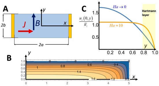
Figure 1.
MHD flow in a long conduit with a rectangular cross-section . The z-coordinate is directed into the paper. (A) Conduit’s cross-section. Current injecting electrodes form the conduit’s side walls (). (B) Contour lines of the normalized axial velocity in the absence of induction (Ha→0). (C) The normalized velocity profile as a function of y/b when the Hartmann (Ha) number is small (blue, Ha→0) and when Ha = 10 (gold). High Hartmann numbers are, however, uncommon but not impossible [5], in electrolytes.
There are a few parallels between electrolytes (in the presence of a supporting electrolyte) and liquid metals, as well as many important differences. In the presence of supporting electrolyte, the liquid conductivity is nearly uniform, like in liquid metals, and the mathematical model is greatly simplified. In contrast to liquid metals, however, the conductivity is small, which results in small body forces, small Reynolds numbers, and small Hartmann numbers. Inertial effects and induction are often not important and the flows are laminar.
In contrast to liquid metals, ions, not electrons, conduct electricity in electrolytes. Many of the challenges with electrolyte-based MHD are related to the electrodes’ chemistry. This review focuses on aqueous solutions. In closed systems, one must operate with a sufficiently low potential difference between the electrodes, typically below ~1.2 V, to avoid water electrolysis that would cause accumulation of gas bubbles at the electrodes’ surfaces. Such gas blankets reduce the effective area of the electrodes and may cause clogging in microfluidic conduits. Operation at high electrode potential differences requires means to vent vapor. To address this challenge, Homsy et al. [16,17] positioned the current-injecting electrodes in vented chambers located outside the flow conduit but in electrical communications with the MHD conduit/pump. Bubbles that formed next to the electrodes never entered the flow conduit and were vented to the atmosphere. Even in the absence of water electrolysis, electrochemical reactions may lead to electrodes’ corrosion, reducing the useful life of such devices and to alternations in the electrolyte’s pH, which may affect chemical reactions and biological interactions.
Many of the unwanted effects associated with electrode chemistry can be alleviated by operating with RedOx species such as FeCl2/FeCl3, or ferri- and ferro-cyanide, which undergo reversible reactions at the electrodes [14,18,19]. RedOx electrolytes facilitate relatively high current fluxes at low electrode potential differences, do not form any reaction byproducts at the electrodes’ surfaces, and do not cause electrode corrosion (when inert electrodes are used). Unfortunately, many common RedOx species are strong oxidizers that may be incompatible with biological matter and processes.
Another remedy to minimize adverse effects of electrodes’ electrochemistry is to operate with AC electric fields. However, a change in the direction of the electric field results in a change in the direction of the Lorentz force and of the flow. When steady, unidirectional flow is desired, one must alternate the magnetic field in sync with the electric field [20,21]. When AC electric and magnetic fields are used (AC-MHD), the magnetic flux density () and the current flux () vary periodically in time with angular frequency and phase lag , resulting in the steady component of the Lorentz body force . Some of the disadvantages of AC operation are the need to use electromagnets (instead of zero-power-consuming permanent magnets); the induction of parasitic currents (due to the time-alternating magnetic fields); and significant heating (especially at high frequencies). AC operation may, however, provide an opportunity to induce electrical currents via capacitive coupling, avoiding/minimizing electrochemical reactions and minimizing large drops in potential in the electric double layers.
Yet another alternative that does not involve any electrical contact with the liquid is induction pumping with a travelling wave magnetic field along the conduit’s length. The applied magnetic field induces currents in the liquid, which in turn interact with the magnetic field. In the presence of appropriate phase lag, the resulting Lorentz force propels the liquid [22]. This mode of operation is, however, more appropriate for liquid metals than electrolyte solutions.
3. MHD (Hartmann) Conductive Pumps and Thrusters
In microfluidic systems, it is often necessary to move conductive liquids (electrolytes) around. MHD provides a convenient means to generate body forces and propel liquids compactly without a need for any moving, mechanical members. Likewise, MHD can be used to propel micro-swimmers, particularly when the magnetic and/or the electrostatic fields are externally applied.
Julius Hartmann (1937) was the first to investigate (around 1915), theoretically and experimentally, how a DC magnetic field affects pressure-driven flow of a conducting liquid (mercury) between two parallel plates with distal blocking side electrodes [23]. In Hartmann’s case, the interaction between the moving conductor and the magnetic field produced emf and a Lorentz body force that opposed the pressure-driven flow (Hartmann break). In contrast, here I examine a conductive MHD pump, wherein the electrodes inject current into the conducting liquid to produce the Lorentz body force. For simplicity, I consider abundance of supporting electrolyte that renders the liquid conductivity σ (S m−1) nearly uniform. Consider a long conduit with a rectangular cross-section (−a < x < a, −b < y < b, a > b) (Figure 1). The conduit’s axis is aligned with the z-direction. The conduit’s side walls are electrodes with the potential difference ΔV. These electrodes inject current flux . is a unit vector in the x-direction. The surfaces are insulating. In the presence of a uniform magnetic field , the Lorentz body force JB0 propels the fluid in the z-direction. I assume a small Reynolds number, a small Hartmann number, and non-slip velocity at all solid surfaces .
When the conduit is long L >> b, far from the conduit’s inlet and exit, the flow is fully developed with the constant pressure gradient and z-independent axial velocity . Numerical simulations provide information on the development length needed to achieve fully developed conditions [24].
The fully developed, velocity profile of the resulting MHD flow in the presence of uniform current flux J and uniform magnetic field B is obtained by solving Equation (14). The resulting velocity profile is like the velocity profile of fully developed, pressure-driven flow [25]:
The cross-section averaged velocity is:
where:
When the Hartmann number is small and a >> b, the velocity profile is parabolic in the y-direction and flat along most of the x-direction; except next to the sidewalls (), where the velocity decreases to zero within layers of thickness b (Figure 1B,C). That is, the effect of the side walls is screened by the conduit’s floor and ceiling. The MHD pump’s stagnation pressure gradient is .
Like the pressure force, the Lorentz force scales with the conduit’s volume while the viscous force scales with the conduit’s surface area. When operating under galvanic (current control) conditions, as the conduit cross-section’s dimensions decrease, so do the maximum fluid velocity and the flow rate. Often, however, to avoid unwanted electrodes’ electrochemical reactions, one constrains the potential difference ΔV between the electrodes. Consider a rectangular cross-section with a fixed potential difference between the opposing, current-injecting electrodes (Figure 1A). When a >> b, as the distance between the electrodes (2a) decreases, the electric current flux J = σ ΔV (2a)−1 increases while the wall shear stress, which is controlled by the conduit’s height b, decreases. Thus, when the electrodes potential is controlled (potentiometric conditions), as (a) increases, the maximum velocity in the conduit increases, attains a maximum, and then decreases to zero. When b/a << 1, the maximum velocity is proportional to (a/b). As (a) increases, the volumetric flow rate increases and eventually reaches an asymptote (Figure 2).
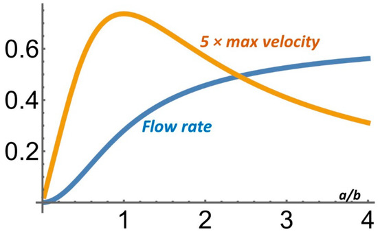
Figure 2.
A MHD pump operating under potentiometric conditions in the absence of a pressure gradient and with the potential difference ΔV across the electrodes. The dimensionless maximum velocity and the dimensionless flow rate are depicted as functions of the aspect ratio a/b. When a/b- > 0, the maximum velocity ~a/(4b).
Here, I examine a relatively simple conduit cross-section’s geometry amenable to an analytical solution. More complex conduit cross-sectional geometries or electrode placements would require numerical simulations. More generally, the MHD’s pump flow rate (Q) is the superposition of the Lorentz force-driven flow and the pressure-driven flow:
where Hp and HL are, respectively, the hydraulic conductivities associated with the pump’s pressure head and the Lorentz body force. In the above, Δpadv is the adverse pressure difference between the conduit’s exit and inlet and ΔV is the potential difference between the current injecting electrodes. In the case of the conduit of Figure 1A, and . The maximum flow rate takes place when there is no adverse pressure Qmax = HLΔV. The maximum pressure head created by the pump is the stall pressure . We can rewrite Equation (18) as:
The mechanical power produced by this MHD pump:
is maximized when and . That is, . Often, the pump’s efficiency is defined as the ratio between the maximum pump’s mechanical power and the electrical power consumed (IΔV). . The efficiency of the pump of Figure 1 is:
In the above, I used (a) as the length scale in the Hartmann number. The pump’s efficiency is proportional to the square of the Hartmann number. Since electrolyte’s Hartmann number is often small, so is the efficiency of MHD pumps operating with electrolytes.
By judicious adjustment of electrodes’ potentials/current, the MHD pump can double as a valve to block pressure-driven flow. I will take advantage of this dual characteristic of the pump in the next section, where I discuss MHD networks.
As discussed in Section 2, the current flux intensity in MHD pumps operating with electrolytes is severely limited by adverse effects of electrode electrochemistry. These adverse effects can be partially alleviated by placing the electrodes outside the flow conduit to minimize interference from bubble formation [16,17]; by operating with RedOx couples that undergo reversible electrochemical reactions at the current injecting electrodes without producing undesired byproducts [14,18,19]; and by operating with synchronous AC current and AC magnetic field [20,21]. Yet another idea is to use an AC electric field, a DC magnetic field, and a flow rectifier [26], such as a nozzle-diffuser-shaped conduit, so that the forward flow encounters a smaller hydraulic resistance than the backward flow. However, since the Stokes flow is time-reversible, significant biased flow is achievable only when inertial effects are significant (Re >> 1).
An emerging application for MHD micropumps is in electronic cooling [27,28]. High-power density converters require liquid cooling to enhance heat dissipation. MHD pumps operating with room temperature liquid metals, such as gallium alloys, are attractive since the MHD pump can be integrated into the power converter, eliminating the need for both an external magnet and an external power supply [28].
When the device containing the MHD conduit is free to move, we have a MHD thruster that can propel a swimmer such as a submarine [3] or a micro-swimmer. The MHD flow can be either internal or external to the swimmer. The thrust can be generated either by transferring momentum to the liquid or by direct application of the Lorentz force to the swimmer, wherein ion current in the fluid is a part of the electrical circuit. As an example of the latter, Salinas et al. [29] designed, constructed, and tested an autonomous swimmer comprised of electrically connected Mg and Pt electrodes (e.g., a Janus particle). When submerged in an acidic solution, the Mg is oxidized at the anode and H3O+ is reduced at the Pt electrode. This interaction results in an ionic current in the suspending solution between the Mg and Pt electrodes and an electron current in the conductor that connects the Mg and Pt electrodes. In the presence of a uniform magnetic field such as provided by a permanent, rare-earth magnet, the ionic current interacts with the magnetic field to produce two counter-rotating vortices around the electrodes. In addition to hydrodynamic effects, the swimmer is subject to Lorentz force resulting from the interaction between the electron current transmitted in the solid and the externally applied magnetic field.
Al-Habahbeh et al. [30] provide an extensive list of publications on MHD micro- and macro-pumps, thrusters, and applications. The mathematical model presented in this section assumed uniform electrolyte conductivity and did not account explicitly for electrode electrochemistry. A few researchers [24,31,32,33] included the calculation of the concentration fields of the various ionic species and electrode electrochemistry in the modeling of MHD pumps. Such models are necessary to obtain accurate predictions and insights but are complicated by the need to solve multiple Nernst–Planck equations (Equation (5)), one for each species, and address non-linear electrode kinetics (e.g., Butler–Volmer kinetics) and often require numerical methods.
4. MHD Networks
An interesting extension of the MHD pump concept is MHD networks. Imagine a network of conduits (Figure 3), each of which is equipped with a couple of individually controlled electrodes, as shown in Figure 1A. Each branch of the network acts as either a pump or a valve. By judicious control of the electrodes’ potentials, fluid flow in this network can be directed to follow any desired path, including circulation in one or more closed loops [34], just like current flow can be directed in an electrical circuit by controlling the potential differences across individual network branches.
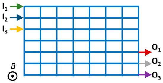
Figure 3.
A schematic depiction of a MHD network. Each branch of the network comprises a conduit equipped with a pair of individually controlled electrodes (like in Figure 1A). The network may accept samples and reagents through multiple inlets (Ik) and discharge reaction products via outlets (Ok). By judicious control of individual network branches’ electrical potentials, one can drive fluid flow in the network along any desired path between inlets and outlets; circulate fluids along closed internal paths to expose the fluid to various incubation temperatures; and mix and react various flow streams [34].
When potential differences in individual legs of the network are specified, the flow rate through each leg can be predicted by solving the corresponding Kirchhoff’s laws. This can be readily done with software tools equipped with a graphical user interface (GUI) such as the SPICE software for electronic circuit design, wherein electric currents are surrogates for the flow rates of our MHD network, or with MHD Nets software specifically written for MHD circuits [35]. Alternatively, in the control mode, one can compute the electrodes’ potentials needed in each branch of the network to direct fluid flows along any desired paths. Such a network can accommodate concurrent flow processes. The MHD network provides a convenient, inexpensive means for flow control without a need for any mechanical components. Furthermore, individual elements can be equipped with resistor heaters to provide desired incubation temperatures. Such networks can be used to facilitate various unit operations as needed for lab-on-chip technology, including merging and mixing of flow streams, and circulating liquids among various temperature zones, as well as providing on-demand cooling for thermal control.
The MHD networks described above can be conveniently manufactured with printed circuit boards combined with conduits molded in Polydimethylsiloxane (PDMS). Alternatively, as in our lab, one can use low-temperature co-fired ceramic (LTCC) tapes. LTCC tapes comprise ceramic particles and glass frit embedded in a polymeric material. In their green state, the (about 100–400 mm thick) tapes are soft, pliable, and amenable to cutting to form networks of conduits and to screen-printing of thick films to form electrodes, electrical interconnects, resistors, and other passive electronic components. Multiple layers of green tapes are stacked together with vias providing connections among layers. The tapes are then co-fired, the polymer burns out, and the ceramic particles sinter to form a rigid, three-dimensional structure with embedded networks of conduits, electrodes, and interconnects [34,36,37].
In addition to applications in lab-on-chip technology, MHD networks can be used to, among other things, provide on-demand cooling for high density electronic circuits, wherein liquid is circulated only through hot spots. Such networks can operate with either aqueous solutions or with room-temperature liquid metals such as gallium alloys.
5. MHD Actuators
Consider a rigid rectangular cavity (−a < x < a, −b < y < b) filled with a conducting fluid (e.g., like in Figure 1A), equipped with electrodes at , and subjected to a uniform magnetic field () in the z-direction (perpendicular to the page). When a potential difference is applied across the electrodes, current of density flows in the electrolyte solution. This current induces the Lorentz body force . When , the Stokes Equation (14) admits the no-motion state: or . That is, the Lorentz body force is balanced by the hydrostatic pressure without inducing any liquid motion.
When the cavity floor and/or ceiling are compliant, this Lorentz body force may cause these surfaces to deform, providing actuation. This is like the operation of a rail gun. Since electrolyte solutions usually carry only low current, this effect would be more pronounced if the electrolyte were replaced with a liquid metal.
Fluid flow in such a cavity can be induced in the presence of a non-uniform current such as when different regions of the cavity are subjected to electrical currents in different directions or in the presence of a spatially non-uniform magnetic field. Figure 3 depicts a cavity with an array of individually controlled electrodes patterned on its bottom. By controlling the potential differences across pairs of electrodes, it is possible to induce either unidirectional current in the cavity or currents with alternating directions. In the presence of uniform axial electric current, there is no flow in the conduit filled with an electrolyte solution and exposed to an electric field as indicated by the stationary, straight streak on dye (Figure 3 top). In the presence of nonuniform current spins the liquid, introducing circulation (Figure 4 bottom) [38].
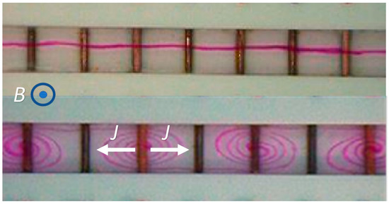
Figure 4.
A conduit equipped with transverse electrodes, filled with electrolyte solution, and subjected to a uniform magnetic field. The figure illustrates the deformation of an initially straight line of dye [38] (Top) placed at the conduit’s mid-height in the absence of potential differences among the electrodes. (Bottom) Potential differences applied to the vertical electrodes induce electrical currents (J) with opposite directions that, in the presence of the magnetic field, result in Lorenz forces in opposing directions and in flow circulation, as is evident from the deformation of the dyed line.
By judicious patterning of the current injecting electrodes in the presence of magnetic fields, it is possible to actuate complex flow patterns (Figure 4 bottom), [38,39]. Such actuators can be used to, among other things, control flow instabilities and stir liquids (Section 7).
Active flow control and suppression of flow instabilities in boundary layers are of interest in marine propulsion and in aircraft. In marine applications, the hull’s surface can be patterned with magnets and electrodes to induce Lorentz forces in the boundary layer to delay boundary layer separation and/or transition to turbulence, thereby reducing drag [40,41]. A similar approach can be applied to aircraft, wherein the patterned electrodes inject current and, when necessary, ionize the air.
6. Magneto Electrochemical Hydrogen Production and Power Conversion
Consider the conduit with a rectangular cross-section (Figure 1A) equipped with electrodes at positions . When externally imposed pressure gradient drive electrolyte flow in this conduit in the presence of a magnetic field, the Lorentz force acts on the oppositely charged cations and anions in opposite directions, leading to charge separation and to electromotive force emf. When the electrodes are blocking, a Faraday–Hall potential difference develops across the electrode pair. The magnitude of this potential difference is proportional to the flow rate. This is essentially the principle of operation of electromagnetic flow meters [2].
When the electrodes are connected to an external load, current will be transmitted through this load, thereby carrying out work. In other words, such a process converts the mechanical work used to pump the fluid into electrical work [42,43]. Since electrolytes typically have low electric conductivity, the conversion efficiency is low, and liquid metals are more suitable for power conversion. As a potentially added benefit in the case of electrolytes, the electrochemical reactions at the electrodes produce hydrogen gas (when the electrolyte is aqueous) and chloride gas (in the presence of Cl- ions) that can be then harvested [42]. The current transmitted in the electrolyte interacts with the magnetic field to produce a Lorentz force that opposes the electrolyte flow (Hartmann break).
7. MHD Stirrers
MHD provides a convenient means to stir liquids to enhance mass transfer, chemical reactions, and biological interactions. One can pattern electrodes of various shapes to induce electric fields in different directions. These electric fields then interact with the magnetic field to produce fluid circulation. To make the ideas involved more concrete, let us reconsider the flow conduit of Figure 1A. In addition to the “pumping” electrodes placed along the conduit’s side walls, we equip this conduit with individually controlled, point (circular) electrodes positioned along the conduit’s axis and denoted Ak in Figure 5A. During the pumping operation, the electrodes Ak are silent. When stirring is desired, the electrodes located at the conduit’s side walls are interconnected to form the single electrode S. When a potential difference is applied between one of the internal electrodes, say A0, and the side electrode S, electric current flows radially from A0 to S. In the presence of a magnetic field, the Lorentz force is in the azimuthal-direction and induces circulation around the electrode A0 (Figure 5A), which brings material from one half of the conduit to its other half [44]. Since, typically, the Reynolds number associated with these types of flows is small, the flow is laminar and the stirring is poor, as shown in the theoretically calculated trajectories of passive tracers (Figure 5B). Material can be transported across streamlines only by diffusion, which is a slow process. Matters can be greatly improved by alternating the potential difference between two or more Ak–S pairs. For example, electrode pairs A1-S and A-1-S are programmed to induce counter rotating vorticities. Each electrode pair produces flow fields such as the one shown in Figure 5A. By alternating between these two or more well-ordered flow fields, we subject a blob of dye to continuous stretching and folding, producing Lagrangian Chaos and high-efficiency stirring (Figure 5C). Figure 5C depicts snapshots of the stretching and folding of the blob of dye as predicted and observed in our experiment [44]. The theoretical predictions are obtained by solving the Stokes equation (Equation (14)). Witness that, within a few cycles, the blob of dye spreads uniformly throughout the fluid as is desired for an effective stirring [44].
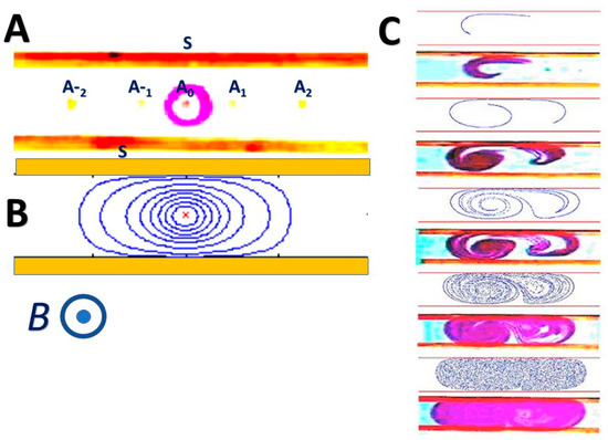
Figure 5.
An example of a MHD stirrer [44]. (A) The conduit of Figure 1A is equipped with electrodes along its side walls and point electrodes located along its axis and denoted Ak. The electrodes along the side walls are connected and denoted S. When a potential difference is applied between the central electrode A0 and the side wall electrode S, fluid circulation results as shown with dye (A) and in theoretical predictions (B). By alternately engaging the two agitators A-1-S and A+1-S, the device alternates between two flow patterns, resulting in chaotic advection (Lagrangian Chaos) and efficient stirring (C). The image (C) depicts observations of the evolution of a blob of dye in theoretical simulations and in experiments.
The flow structures are dictated by electrode patterns, which offer a great amount of flexibility in stirrer design [38,45,46]. For example, Yi et al. [45] describes a stirrer comprised of a circular cavity whose circumference acts as an electrode and two inner eccentric electrodes (agitators) placed flush with the cavity’s floor. When a potential difference is applied between one of the inner electrodes and the circumference, circulatory flow results. When the two inner electrodes are alternately actuated, chaotic advection results, as in Figure 5C. Moreover, the circumferential electrode can also be flush with the device’s floor to form a virtual flow conduit without any rigid walls [47].
The ease with which one can reverse the direction of the Lorentz force enables an alternative design of MHD stirrers. Gleeson et al. [48,49] constructed a toroidal MHD stirrer, one half of which is filled with liquid A and the other half with liquid B. MHD drives the flow in the torus. As a result of the parabolic velocity profile associated with MHD flow (Figure 1B), one liquid penetrates into the other, increasing the interface area between liquids A and B. The flow is then reversed and the process is repeated. The net result is formation of thin interpenetrating lamellas that shorten the diffusion distances of fluids A and B (Taylor–Arris dispersion). Similar ideas can be adapted for various material processing applications.
8. MHD Chromatograph and MHD PCR Machine
Liquid chromatography (LC) is used for the separation, purification, and detection of various species. Typically, LC requires the pumping of mobile phase—a carrier fluid laden with various analytes—through a long column coated with a stationary phase. Since different analytes differ in their affinities to the stationary phase, as the solution flows through the column, various species are separated into distinct bands. The column’s length needed for efficient separation depends, among other things, on the affinities of the analytes that need to be separated. For example, when protein A and protein B have very diverse affinities to the stationary phase, a short column may suffice. In contrast, when the affinities of A and B with the stationary phase are similar, a long column is needed.
Existing LCs comprise a fixed length column. This shortcoming can be alleviated with a column that forms a closed loop of virtually an “infinite” length, enabling one to probe the separated species in nearly real time during the separation process and terminating the process once a desired level of separation has been achieved. MHD is one of the few methods that enables continuous circulation of fluid in a closed loop [37,50,51]. A few researchers [50,51] experimentally studied a circular AC MHD-LC, demonstrating a separation rate of 0.2 plates/s and hypothesizing the possibility of much larger separation rates with appropriate optimization. The disadvantages of MHD LC include low flow rates (resulting in low separation rate); alternations in pH resulting from electrodes’ electrochemistry; possible bubble formation; and susceptibility to Taylor–Arris dispersion (band broadening) when operating with non-uniform velocity profile in an open column. A relatively flat velocity profile is attainable with a packed bed column or when the Hartmann number is large, which is unlikely with electrolytes.
MHD-based Continuous PCR: The polymerase chain reaction (PCR) is commonly used in biotechnology for, among other things, nucleic acid amplification for genetic analysis and for diagnostics. To facilitate DNA amplification, one mixes a sample containing target DNA with the appropriate reagents and alternates the reaction volume temperature among three values. Most PCR processes are carried out with the sample placed in a stationary reaction chamber or a test tube and the temperature of the reactor cycled. This arrangement necessitates the heating and cooling of both the reaction mix and the surrounding substrate, which is power-consuming and slow due to the substrate’s high thermal inertia. In the alternative process of continuous flow PCR, the reaction mix is cycled continuously among three zones maintained at three different, fixed temperatures. Since only the small mass of the reaction mix is subjected to temperature alternation, this process is much more energy efficient and faster than in the conventional PCR. Here, MHD’s ability to circulate fluid in a closed loop is again an advantage. West et al. [21] constructed MHD-PCR to continuously circulate the PCR mix in a closed loop with three heaters, creating three distinct regions at the temperatures needed for DNA denaturation (~94 °C), annealing (50–55 °C), and extension (72 °C). PCR amplification has been, however, challenged, perhaps due to adverse effects of electrodes’ electrochemistry. Similar ideas can be applied to other chemical processes that require temperature alternations and may be less sensitive to byproducts of electrodes’ electrochemistry. Interestingly, closed loop continuous PCR has been successfully demonstrated with buoyancy as the driving force [52].
9. MHD Propulsion of Liquid Slugs
Thus far, we have discussed MHD pumping in the absence of interfaces. In certain applications, it is desirable to propel liquid slugs and droplets. In these cases, the Lorentz forces must overcome capillary forces, contact line resistance, and contact angle hysteresis. Both capillary forces and viscous drag scale with the surface area, while the Lorentz force scales with the volume. This makes the use of MHD at sub-mm length scales challenging.
Liquid–air interface occurs, for example, in optical switches. Such a switch comprises a fluid conduit that intersects a solid optical waveguide at an angle greater than the total reflection angle [53]. The switch changes from the off position (total reflection) to the on position (light transmission) by replacing a fluid with a low index of refraction, such as air, in the light’s path with an electrolyte that has the same index of refraction as the solid waveguide and allows complete light transmission. Miao et al. [53] achieved this feat with an MHD drive that replaces the electrolyte with air and vice versa [53]. Here, the Lorentz forces must overcome both a pressure head and the resistance posed by capillary forces at the electrolyte–air interface; a resistance that can be substantial at the microscale.
Another intriguing application of MHD is in digital microfluidics. In digital microfluidics, individual liquid drops serve as minute chemical/biological reactors that are propelled within a device among different locations such as incubation, mixing, and sensing stations. Furthermore, drops can be mixed, fused, and split. Typically, in digital microfluidics, the droplets are propelled by modulating the substrate’s surface energy locally with electric fields (electrowetting). Droplets migrate in such a way as to decrease surface energy. Droplets can also be propelled and fused and undergo fission with Lorentz forces. Consider a surface patterned with individually controlled, point electrodes (Figure 6). By applying potential differences across pairs of electrodes, one can transmit electric current in the conducting droplets. In the presence of a magnet, these currents interact with the magnetic field and propel the droplets. Figure 6 (unpublished data) depicts, from left to right, two droplets propelled towards each other until they fuse. These two droplets can carry different chemicals or reagents and their fusion would enable chemical/biological reactions. Furthermore, by judicious actuation of the electrodes, one can induce internal circulation in the fused droplet to enhance mixing. Droplets can also be transported among stations at various temperatures and, in addition to being fused, can be split into daughter droplets.
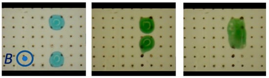
Figure 6.
Digital microfluidics with MHD. The device’s surface is patterned with individually controlled electrodes. The device is exposed to a magnetic field provided by a permanent magnet. When a potential difference is applied to pairs of electrodes at the drops’ locations, the resulting current interacts with the magnetic field to produce Lorentz forces, causing the drops to migrate. This image depicts two drops migrating towards each other until they fuse. By judicious programming of the electrodes, one can move droplets along any desired path, induce stirring in the drops, cause two or more drops to fuse, and split drops (unpublished work).
During droplet propulsion, the contact angles at the droplet’s fore is larger than at its rear. This contact angle hysteresis presents a significant resistance to drop propulsion. This resistance can be reduced, however, with the use of super hydrophobic surfaces.
In the propulsion method described above, the electrodes inject current into the droplet. This requires the droplet to be in contact with electrodes. When the droplet is highly conductive (e.g., liquid metal), it is possible to induce eddy currents in the drop with a time-varying magnetic field (Equation (8)) and without a need for electrodes. These eddy currents then interact with the externally applied magnetic field to produce Lorentz body forces that induce fluid motion in the droplet and propel the droplet [54]. The time-varying magnetic field can be produced with an electromagnet or with a translating permanent magnet.
10. Magnetic Resonance Imaging (MRI)
MRI has revolutionized medical diagnostics, enabling high resolution imaging of soft tissues without exposure to ionizing radiation, and is increasingly used in surgery (interventional MRI). MRI machines in current use are considered safe. Millions of MRI scans are performed annually worldwide with very few adverse events, most of which involve heating and/or burns. The trend is, however, to increase the magnetic field intensity of (A) MRI machines to improve image quality and reduce noise to signal ratio [55], and of (B) magnets used to position and control nanorobots for minimally invasive surgery [56]. The magnetic field used in MRI comprises of the ever-present static field (B0), with magnetic flux density as high as 12T in research machines, and time varying fields: the audio-frequency gradient field for spatial encoding and the RF field for magnetic resonance excitation. Since body fluids such as blood are electrolytes, the effect of magnetic fields on body fluids during MRI is under the purview of magneto electrochemistry.
The MRI’s AC magnetic field induces electrical currents and Joule heating in tissue and body fluids (Equation (8)) and can be used for therapeutic hyperthermia. The potential effects of the DC magnetic field B0 have attracted less attention. B0 may, among other things, interact with intracellular and extracellular electrical currents and with neuron signaling; affect blood rheology (decrease or increase apparent blood viscosity) [57]; affect wall shear stress (Figure 1C, Ha > 1) and mobile ion distribution; and induce electrical currents, body forces, and Joule heating in moving conductors such as blood.
Using finite element numerical simulations, Kinouchi et al. [58] found that the aortic blood flow decreases by 2% (consistent with Gold’s analysis [59]) and 5% in the presence of an insulating and conductive artery, respectively, in a steady magnetic flux of 10 T. This relatively small effect of the magnetic field B0 on the blood flow rate and wall shear stress [60] is consistent with the small corresponding Hartmann number (Ha). When the blood conductivity σ~0.3 S m−1 and viscosity 3 m Pa s, B0 = 10 T, and the radius of the blood vessel is 10−2 m, the corresponding Hartmann number is approximately 0.1.
Finally, since blood vessels are electrically conducting, the emf produced by blood flow in the presence of the MRI’s magnetic field affects electrocardiogram (ECG) recordings. This is something that needs to be accounted for to correctly interpret ECG signals but which can also be exploited for noninvasive blood flow rate measurements by correlating electrocardiogram (ECG) readings during MRI’s static magnetic field (B0) with blood-flow-induced emf [61]. Intriguingly, inspired by MHD marine propulsion, a few inventors (e.g., [62]) proposed MHD pumps to assist the heart in pumping blood following damage to the heart muscle. Superficially, MHD pumps appear attractive since electrodes can be placed in major blood vessels with a minimally invasive catheter. However, the abovementioned inventors do not appear to have considered the adverse effects of electrochemical processes at the current-injecting electrodes. This is likely one of the reasons why MHD blood pumps have not been used in practice.
11. Concluding Remarks
Magnetic fields affect conducting liquids such as liquid metals, electrolytes, and suspensions of paramagnetic particles in multiple ways. Uniform magnetic fields polarize and align paramagnetic and diamagnetic suspended particles, causing aggregation and modifying suspensions’ rheological properties, a phenomenon dubbed magneto-rheology. Magnetic field gradients polarize paramagnetic/diamagnetic particles and induce particles’ migration (magnetophoresis). Time-varying magnetic fields induce eddy currents in conductors and Joule heating. Localized heating of particles can be used to catalyze chemical reactions, facilitate drug delivery, and destruct malignant cells (hyperthermia).
When an electrical current (e.g., provided by a power supply) is transmitted in a conductor, such as an electrolyte, in the presence of an applied magnetic field, the electrical current interacts with the applied magnetic field to produce the Lorentz body force. An electrical current can also be induced in a conductive medium with a time-varying magnetic field. The Lorentz body forces produce pressure gradients in the fluid and can drive fluid motion, referred to as magnetohydrodynamics (MHD). Conversely, a conductive fluid flowing in the presence of a magnetic field experiences charge separation and electromotive force (emf). A pair of electrodes submerged in the fluid parallel to the direction of the flow and the direction of the magnetic field will sense a potential difference (emf) with a magnitude that is proportional to the flow rate. This is the principle of electromagnetic flow metering. When the electrodes are connected to an external load, this emf induces current through the solution and the load, thereby converting mechanical (flow) power into electrical power and, in some cases, producing electrochemical reaction products such as hydrogen that can be harvested. Furthermore, the induced electric current interacts with the magnetic field to produce Lorentz body forces that may oppose (Hartmann break) the externally driven flow in certain regions and enhance the flow in other regions, thereby flattening the velocity profile. In electrolyte solutions, one can neglect the effect of electrical currents on the externally applied magnetic fields. That is, the magnetic field can be determined independently of the flow field.
This review focuses on the interactions among electric fields, magnetic fields, and flow fields when the fluid is an electrolyte. Magneto electrochemistry (MEC) is not new. It dates to Faraday, who attempted to measure the emf induced by the Thames River flow in the presence of the Earth’s magnetic field. Many researchers examining the interactions of electrolytes with magnetic fields have treated the electrolyte like an ohmic conductor, similar to liquid metals. There are, however, important distinctions between electrolytes and liquid metals. In electrolytes, electrochemical (Faradaic) reactions take place at the current-injecting electrodes. These electrochemical reactions are rate-limiting and often produce unwanted products such as alternations in solution pH, and gas bubbles that reduce the effective area of the current-injecting electrodes and that alter flow patterns. Bubble formation in microfluidic systems is particularly problematic as bubbles can clog flow conduits. Furthermore, ions’ concentrations are often spatially dependent; the electrical conductivity is non-uniform; and mass transfer and momentum transport processes are coupled, which complicates theoretical treatments. There are only a few theoretical studies that account for the transport of ionic species in the electrolytes in the presence of magnetic fields. To obtain accurate predictions [13], gain insights, discover new phenomena, and identify new applications, it is necessary to address the coupled processes of individual species’ mass and momentum transport in electrolytes, as elucidated in Section 2.
In many electrochemical processes such as in batteries, electroplating, electro-machining, and voltammetry, electrical currents are an essential part of the process. When these processes are carried out in the presence of a magnetic field such as provided by a permanent magnet, the Lorentz body forces induce fluid motion and enhance mass transfer. This is often with beneficial effects such as increased process speed, smoother and denser plated surfaces, smoother etched surfaces, and suppressed dendrite formation. MHD also facilitates control of surface morphology [63,64,65].
When current is injected into the electrolyte in the presence of a magnetic field to induce fluid motion, the products of the electrochemical reactions are often problematic, primarily due to bubble formation and alternations in solution pH. In the presence of DC magnetic and electric fields, one needs to operate at low enough potential differences to minimize bubble formation, which limits the driving forces. The current flux can be increased and bubble formation eliminated/suppressed with the use of RedOx pairs that undergo reversible electrochemical reactions at the current injecting electrodes. The challenge is, however, to identify RedOx species that are biocompatible and that do not inhibit enzymatic processes such as polymerase. Another means to reduce adverse effects of electrode electrochemistry is to operate with a synchronized AC magnetic field and AC electric field. In this case, the roles of the electrodes alternate, minimizing adverse effects of the products of electrochemical reactions and reducing the potential losses in the electric double layers next to the electrodes. Furthermore, AC operation reduces reliance on Faradaic reactions since current can be transmitted from the electrodes to the electrolyte via capacitive coupling. One could envision operating with blocking electrodes, eliminating electrochemical reactions all together. The use of AC fields complicates, however, system design, and increases power dissipation due to parasitic currents and Joule heating.
Magneto electrochemistry offers an elegant, inexpensive, flexible, customizable, programmable means of performing functions such as pumping and stirring, controlling liquid flow in microfluidic networks, and propelling microparticles without any moving components. To date, most of the applications of MHD in microfluidics have focused on single components such as pumps to induce fluid motion and stirrers to enhance mixing. One can, however, manufacture programmable MHD networks, in which each branch is individually controlled [34], enabling one to circulate fluids along any desired path. Such networks can be used to integrate numerous unit operations in a single device or provide cooling on demand. The MHD net technology is still awaiting applications. Adverse effects of electrode electrochemistry, bio-incompatibility of RedOx species, and complexity of synchronous AC operation are likely the major barriers to the adaptation of MHD technology in microfluidic devices.
Funding
The work was supported, in part, by DARPA’S SIMBIOSYS PROGRAM through grant N66001-01-C-8056 to the University of Pennsylvania.
Institutional Review Board Statement
Not applicable.
Informed Consent Statement
Not applicable.
Data Availability Statement
Not applicable.
Conflicts of Interest
The author declares no conflict of interest.
References
- Davidson, P.A. Cambridge texts in applied mathematics. In An Introduction to Magnetohydrodynamics; Cambridge University Press: Cambridge, NY, USA, 2001; 431p. [Google Scholar]
- Shercliff, J.A. The Theory of Electromagnetic Flow-Measurement; Cambridge University Press: Cambridge, UK, 1962. [Google Scholar]
- Way, S. Electromagnetic propulsion for cargo submarines. J. Hydronaut. 1968, 2, 49–57. [Google Scholar] [CrossRef]
- Clancy, T. The Hunt for Red October; HarperCollins Publishers: London, UK, 2018. [Google Scholar]
- Andreev, O.; Haberstroh, C.; Thess, A. MHD flow in electrolytes at high Hartmann numbers. Magnetohydrodynamics 2001, 37, 151–160. [Google Scholar]
- Townsend, J.S.E. The diffusion and mobility of ions in a magnetic field. Proc. R. Soc. Lond. A 1912, 86, 571–577. [Google Scholar]
- Cantillon-Murphy, P.; Wald, L.L.; Zahn, M.; Adalsteinsson, E. Proposing magnetic nanoparticle hyperthermia in low-field MRI. Concepts Magn. Reson. Part A Educ. J. 2010, 36, 36–47. [Google Scholar] [CrossRef]
- Qian, S.; Bau, H.H. Magneto-hydrodynamics based microfluidics. Mech. Res. Commun. 2009, 36, 10–21. [Google Scholar] [CrossRef]
- Pamme, N. Magnetism and microfluidics. Lab Chip 2006, 6, 24–38. [Google Scholar] [CrossRef]
- Zhu, G.-P.; Wang, Q.-Y.; Ma, Z.-K.; Wu, S.-H.; Guo, Y.-P. Droplet Manipulation under a Magnetic Field: A Review. Biosensors 2022, 12, 156. [Google Scholar] [CrossRef]
- Gregory, T.S.; Cheng, R.; Tang, G.; Mao, L.; Tse, Z.T.H. The magnetohydrodynamic effect and its associated material designs for biomedical applications: A state-of-the-art review. Adv. Funct. Mater. 2016, 26, 3942–3952. [Google Scholar] [CrossRef]
- Newman, J.; Thomas-Alyea, K.E. Electrochemical Systems; John Wiley & Sons: Hoboken, NJ, USA, 2012. [Google Scholar]
- Qin, M.; Bau, H.H. Magnetohydrodynamic flow of a binary electrolyte in a concentric annulus. Phys. Fluids 2012, 24, 037101. [Google Scholar] [CrossRef]
- Qian, S.; Chen, Z.; Wang, J.; Bau, H.H. Electrochemical reaction with RedOx electrolyte in toroidal conduits in the presence of natural convection. Int. J. Heat Mass Transf. 2006, 49, 3968–3976. [Google Scholar] [CrossRef]
- Qin, M.; Bau, H.H. When MHD-based microfluidics is equivalent to pressure-driven flow. Microfluid. Nanofluidics 2011, 10, 287–300. [Google Scholar] [CrossRef][Green Version]
- Homsy, A.; Koster, S.; Eijkel, J.C.; van den Berg, A.; Lucklum, F.; Verpoorte, E.; de Rooij, N.F. A high current density DC magnetohydrodynamic (MHD) micropump. Lab Chip 2005, 5, 466–471. [Google Scholar] [CrossRef] [PubMed]
- Homsy, A.; Linder, V.; Lucklum, F.; de Rooij, N.F. Magnetohydrodynamic pumping in nuclear magnetic resonance environments. Sens. Actuators B Chem. 2007, 123, 636–646. [Google Scholar] [CrossRef]
- Leventis, N.; Gao, X. Magnetohydrodynamic Electrochemistry in the Field of Nd−Fe−B Magnets. Theory, Experiment, and Application in Self-Powered Flow Delivery Systems. Anal. Chem. 2001, 73, 3981–3992. [Google Scholar] [CrossRef]
- Clark, E.A.; Fritsch, I. Anodic stripping voltammetry enhancement by redox magnetohydrodynamics. Anal. Chem. 2004, 76, 2415–2418. [Google Scholar] [CrossRef]
- Lemoff, A.V.; Lee, A.P. An AC magnetohydrodynamic micropump. Sens. Actuators B Chem. 2000, 63, 178–185. [Google Scholar] [CrossRef]
- West, J.; Karamata, B.; Lillis, B.; Gleeson, J.P.; Alderman, J.; Collins, J.K.; Lane, W.; Mathewson, A.; Berney, H. Application of magnetohydrodynamic actuation to continuous flow chemistry. Lab Chip 2002, 2, 224–230. [Google Scholar] [CrossRef]
- Khripchenko, S.; Khalilov, R.; Kolesnichenko, I.; Denisov, S.; Galindo, V.; Gerbeth, G. Numerical and experimental modeling of various MHD induction pumps. Magnetohydrodynamics 2010, 46, 85–97. [Google Scholar]
- Hartmann, J.; Lazarus, F. Hg-dynamics II. In Theory of Laminar Flow of Electrically Conductive Liquids in a Homogeneous Magnetic Field; Levin and Munksgaard-Ejnar Munksgaard: Copenhagen, Denmark, 1937; Volume 15, p. 7. [Google Scholar]
- Kabbani, H.; Wang, A.; Luo, X.; Qian, S. Modeling RedOx-based magnetohydrodynamics in three-dimensional microfluidic channels. Phys. Fluids 2007, 19, 083604. [Google Scholar] [CrossRef]
- White, F.M.; Majdalani, J. Viscous Fluid Flow; McGraw-Hill: New York, NY, USA, 2006; Volume 3. [Google Scholar]
- Heng, K.-H.; Huang, L.; Wang, W.; Murphy, M.C. Development of a diffuser/nozzle-type micropump based on magnetohydrodynamic (MHD) principle. In Proceedings of the Symposium on Micromachining and Microfabrication, Santa Clara, CA, USA, 20–22 September 1999; pp. 66–73. [Google Scholar]
- Yerasimou, Y.; Pickert, V.; Ji, B.; Song, X. Liquid metal magnetohydrodynamic pump for junction temperature control of power modules. IEEE Trans. Power Electron. 2018, 33, 10583–10593. [Google Scholar] [CrossRef]
- Fan, J.; Zhang, Y.; Wang, J.; Chinthavali, M.S.; Moorthy, R.K. Liquid Metal based Cooling for Power Electronics Systems with Inductor Integrated Magnetohydrodynamic Pump (MHD Pump). In Proceedings of the 2021 IEEE 8th Workshop on Wide Bandgap Power Devices and Applications (WiPDA), Redondo Beach, CA, USA, 7–11 November 2021; pp. 310–315. [Google Scholar]
- Salinas, G.; Tieriekhov, K.; Garrigue, P.; Sojic, N.; Bouffier, L.; Kuhn, A. Lorentz Force-Driven Autonomous Janus Swimmers. J. Am. Chem. Soc. 2021, 143, 12708–12714. [Google Scholar] [CrossRef]
- Al-Habahbeh, O.; Al-Saqqa, M.; Safi, M.; Khater, T.A. Review of magnetohydrodynamic pump applications. Alex. Eng. J. 2016, 55, 1347–1358. [Google Scholar] [CrossRef]
- Qian, S.; Bau, H.H. Magnetohydrodynamic flow of RedOx electrolyte. Phys. Fluids 2005, 17, 067105. [Google Scholar] [CrossRef]
- Qin, M.; Bau, H.H. Magneto-Hydrodynamic Flow in Electrolyte Solutions. 2009. Available online: https://www.comsol.jp/paper/download/44373/Bau.pdf (accessed on 17 October 2022).
- Sen, D.; Isaac, K.M.; Leventis, N.; Fritsch, I. Investigation of transient redox electrochemical MHD using numerical simulations. Int. J. Heat Mass Transf. 2011, 54, 5368–5378. [Google Scholar] [CrossRef]
- Bau, H.H.; Zhu, J.; Qian, S.; Xiang, Y. A magneto-hydrodynamically controlled fluidic network. Sens. Actuators B Chem. 2003, 88, 205–216. [Google Scholar] [CrossRef]
- Zheng, J. Simulation Tools for Magneto-Hydrodynamic (MHD) Networks; University of Pennsylvania: Philadelphia, PA, USA, 2005. [Google Scholar]
- Aguilar, Z.P.; Arumugam, P.; Fritsch, I. Study of magnetohydrodynamic driven flow through LTCC channel with self-contained electrodes. J. Electroanal. Chem. 2006, 591, 201–209. [Google Scholar] [CrossRef]
- Zhong, J.; Yi, M.; Bau, H.H. Magneto hydrodynamic (MHD) pump fabricated with ceramic tapes. Sens. Actuators A Phys. 2002, 96, 59–66. [Google Scholar] [CrossRef]
- Xiang, Y.; Bau, H.H. Complex magnetohydrodynamic low-Reynolds-number flows. Phys. Rev. E 2003, 68, 016312. [Google Scholar] [CrossRef]
- La, M.; Kim, W.; Yang, W.; Kim, H.W.; Kim, D.S. Design and numerical simulation of complex flow generation in a microchannel by magnetohydrodynamic (MHD) actuation. Int. J. Precis. Eng. Manuf. 2014, 15, 463–470. [Google Scholar] [CrossRef]
- Meng, J. Magnetohydrodynamic Boundary Layer Control System. U.S. Patent 5,273,465, 11 February 1993. [Google Scholar]
- Weier, T.; Fey, U.; Gerbeth, G.; Mutschke, G.; Lielausis, O.; Platacis, E. Boundary layer control by means of wall parallel Lorentz forces. Magnetohydrodynamics 2001, 37, 177–186. [Google Scholar]
- De Luca, R. Electromotive Force Generation with Hydrogen Release by Salt Water Flow under a Transverse Magnetic Field. J. Mod. Phys. 2011, 2, 1115–1119. [Google Scholar] [CrossRef][Green Version]
- Ziedan, H.A.; Fayed, I.M.; Abofard, A.E.M. A Novel Design of Water-Flow Based Electrical Generator as an Energy Harvesting Device. MATEC Web Conf. 2018, 171, 02001. [Google Scholar] [CrossRef]
- Qian, S.; Zhu, J.; Bau, H.H. A stirrer for magnetohydrodynamically controlled minute fluidic networks. Phys. Fluids 2002, 14, 3584–3592. [Google Scholar] [CrossRef]
- Yi, M.; Qian, S.; Bau, H.H. A magnetohydrodynamic chaotic stirrer. J. Fluid Mech. 2002, 468, 153–177. [Google Scholar] [CrossRef]
- Qian, S.; Bau, H.H. Magneto-hydrodynamic stirrer for stationary and moving fluids. Sens. Actuators B Chem. 2005, 106, 859–870. [Google Scholar] [CrossRef]
- Sahore, V.; Fritsch, I. Microfluidic rotational flow generated by redox-magnetohydrodynamics (MHD) under laminar conditions using concentric disk and ring microelectrodes. Microfluid. Nanofluid. 2015, 18, 159–166. [Google Scholar] [CrossRef]
- Gleeson, J.P.; West, J. Magnetohydrodynamic micromixing. In Proceedings of the Fifth International Conference on Modeling and Simulation of Microsystems, San Juan, Puerto Rico, 23–25 April 2002; Computational Publications: Cambridge, MA, USA, 2002; pp. 318–321. [Google Scholar]
- Gelb, A.; Gleeson, J.P.; West, J.; Roche, O.M. Modelling annular micromixers. SIAM J. Appl. Math. 2004, 64, 1294–1310. [Google Scholar] [CrossRef]
- Bao, J.-B.; Harrison, D.J. Fabrication of microchips for running liquid chromatography by magnetohydrodynamic flow. In Proceedings of the 7th International Conference on Miniaturized Chemical and Biochemical Analysts Systems, Squaw Valley, CA, USA, 5–9 October 2003. [Google Scholar]
- Eijkel, J.; Dalton, C.; Hayden, C.; Burt, J.; Manz, A. A circular ac magnetohydrodynamic micropump for chromatographic applications. Sens. Actuators B Chem. 2003, 92, 215–221. [Google Scholar] [CrossRef]
- Chen, Z.; Qian, S.; Abrams, W.R.; Malamud, D.; Bau, H.H. Thermosiphon-based PCR reactor: Experiment and modeling. Anal. Chem. 2004, 76, 3707–3715. [Google Scholar] [CrossRef]
- Miao, J.; Wan, J.; Sun, F.; Guo, M.; Wang, Z. Magnetohydrodynamics-based microfluidic optical switch. In Proceedings of the 14th National Conference on Laser Technology and Optoelectronics (LTO 2019), Shanghai, China, 17–20 March 2019; pp. 651–655. [Google Scholar]
- Shu, J.; Tang, S.-Y.; Feng, Z.; Li, W.; Li, X.; Zhang, S. Unconventional locomotion of liquid metal droplets driven by magnetic fields. Soft Matter 2018, 14, 7113–7118. [Google Scholar] [CrossRef]
- Static Magnetic Fields: Report of the Independent Advisory Group on Non-Ionising Radiation; Health Protection Agency: Radiation, Chemical, and Environmental Hazards: Oxfordshire, UK, 2008; Volume 6.
- Nelson, B.J.; Kaliakatsos, I.K.; Abbott, J.J. Microrobots for minimally invasive medicine. Annu. Rev. Biomed. Eng. 2010, 12, 55–85. [Google Scholar] [CrossRef] [PubMed]
- Tao, R.; Huang, K. Reducing blood viscosity with magnetic fields. Phys. Rev. E 2011, 84, 011905. [Google Scholar] [CrossRef] [PubMed]
- Kinouchi, Y.; Yamaguchi, H.; Tenforde, T. Theoretical analysis of magnetic field interactions with aortic blood flow. Bioelectromagn. J. Bioelectromagn. Soc. Soc. Phys. Regul. Biol. Med. Eur. Bioelectromagn. Assoc. 1996, 17, 21–32. [Google Scholar] [CrossRef]
- Gold, R.R. Magnetohydrodynamic pipe flow. Part 1. J. Fluid Mech. 1962, 13, 505–512. [Google Scholar] [CrossRef]
- Drochon, A.; Beuque, M.; Dima, A.-A.R. Impact of an External Magnetic Field on the Shear Stresses Exerted by Blood Flowing in a Large Vessel. J. Appl. Math. Phys. 2017, 5, 1493–1502. [Google Scholar] [CrossRef][Green Version]
- Gregory, T.S.; Murrow, J.R.; Oshinski, J.N.; Tse, Z.T.H. Exploring magnetohydrodynamic voltage distributions in the human body: Preliminary results. PLoS ONE 2019, 14, e0213235. [Google Scholar] [CrossRef]
- Haas, M.J. Bailey, Richard Magnetohydrodynamic Cardiac Assist Device. U.S. Patent US6449959B1, 27 August 2002. [Google Scholar]
- Monzon, L.M.; Coey, J.M.D. Magnetic fields in electrochemistry: The Lorentz force. A mini-review. Electrochem. Commun. 2014, 42, 38–41. [Google Scholar] [CrossRef]
- Wu, Y.; Xu, K.; Zhang, Z.; Dai, X.; Zhao, D.; Zhu, H.; Wang, A. Effect of magnetic field on abnormal co-deposition and performance of Fe-Ni alloy based on laser irradiation. J. Electroanal. Chem. 2022, 905, 115967. [Google Scholar] [CrossRef]
- Shen, K.; Wang, Z.; Bi, X.; Ying, Y.; Zhang, D.; Jin, C.; Hou, G.; Cao, H.; Wu, L.; Zheng, G. Magnetic Field–Suppressed Lithium Dendrite Growth for Stable Lithium-Metal Batteries. Adv. Energy Mater. 2019, 9, 1900260. [Google Scholar] [CrossRef]
Publisher’s Note: MDPI stays neutral with regard to jurisdictional claims in published maps and institutional affiliations. |
© 2022 by the author. Licensee MDPI, Basel, Switzerland. This article is an open access article distributed under the terms and conditions of the Creative Commons Attribution (CC BY) license (https://creativecommons.org/licenses/by/4.0/).