Article

A Distance Measurement Approach for Large Fruit Picking with Single Camera

1
College of Engineering, Huazhong Agricultural University, Wuhan 430070, China
2
Key Laboratory of Agricultural Equipment in Mid-Lower Yangtze River, Ministry of Agriculture and Rural Affairs, Wuhan 430070, China
*
Author to whom correspondence should be addressed.
Horticulturae 2023, 9(5), 537; https://doi.org/10.3390/horticulturae9050537
Submission received: 18 February 2023 / Revised: 6 April 2023 / Accepted: 23 April 2023 / Published: 28 April 2023
(This article belongs to the Special Issue Advances in Intelligent Orchard)

Abstract

:
Target ranging is the premise for manipulators to complete agronomic operations such as picking and field management; however, complex environmental backgrounds and changing crop shapes increase the difficulty of obtaining target distance information based on binocular vision or depth cameras. In this work, a method for ranging large-sized fruit based on monocular vision was proposed to provide a low-cost and low-computation alternative solution for the fruit thinning or picking robot. The regression relationships between the changes in the number of pixels occupied by the target area and the changes in the imaging distance were calculated based on the images of square-shaped checkerboards and circular-shaped checkerboards with 100 cm2, 121 cm2, 144 cm2, 169 cm2, 196 cm2, 225 cm2, 256 cm2, 289 cm2, and 324 cm2 as the area, respectively. The 918 checkerboard images were collected by the camera within the range from 0.25 m to 1.5 m, with 0.025 m as the length of each moving step, and analyzed in MATLAB to establish the ranging models. A total of 2448 images of four oval watermelons, four pyriform pomelos, and four oblate pomelos, as the representatives of large fruit with different shapes, were used to evaluate and optimize the performance of the models. The images of the front were the input, while the imaging distances were the output. The results showed that the absolute error would be less than 0.06 m for both models and would linearly increase with a decrease in the distance. The relative error could be controlled at 5%. The results proved the proposed monocular method could be a solution for the ranging of large fruit targets.

1. Introduction

The picking robot is an effective way to deal with the current challenge of fruit harvest [1,2,3]. Machine vision plays the role of eyes for robots, aircraft technology, the Internet of things, and other mechatronics systems by providing the space coordinate figure [4]. With the location information of the target fruit, the picking robot can perform the supposed work [5,6]. As one of the machine vision methods for target distance assessment, monocular distance measurement has been applied in all sorts of fields, such as industrial robots [7], medical treatment [8], vehicle control [9], and fruit picking [10,11]. Compared to binocular vision and laser vision, it was more convenient and simpler and had great further development potential [12,13].
Initially, it was in the 1960s that research began on monocular vision. Lawrence Roberts at the Massachusetts Institute of Technology (MIT), as the ancestor of monocular vision, obtained a big hit due to the robot’s intelligent recognition through simple building blocks [14]. The following decades witnessed a huge leap again in the monocular field, which paved the way for further development. In 1997, [15] achieved distance calculation according to the proportion of the object’s projection on two images; one was taken at the camera point, while the other was taken at the point where the camera moves along the optical axis. In 2005, [16] proposed a new ranging method in South Korea that used a single camera and a rotating mirror to obtain a series of reflected images through the camera in front of the rotating mirror and extract distance information from them.
Over the course of the last decade, with the boom of new technology, particularly the involvement of computers in machine vision, monocular distance measurement has stepped up to a higher level. In 2013, [17] designed an improved method that used a monocular camera to track specific objects and then employed an efficient computing algorithm implemented in MATLAB/SIMULINK to measure the distance from the object to the camera. In 2017, [18] gave a strategy—a target ranging method for a wheeled mobile robot based on monocular vision—that extended the ranging target from a plane object to a three-dimensional object and improved the measurement accuracy without correction.
In the last 5 years, [19] has used the monocular vision technology of instance segmentation and camera focal length to detect the absolute distance between the front camera and the car camera and has largely improved the measurement accuracy. At the same time, [20] thought the convolutional neural network could be applied to determine the depth from a single camera image; therefore, eight different networks were designed for depth estimation, each of which could suit a certain characteristic level. In 2019, [21] theoretically explored the relationship between local feature correspondence and the similarity of two images. The object will be identified based on a two-stage template matching process, and its proportion level will be determined at the same time. Then it will be successfully applied to the real-time automatic packaging sorting line. In the same year, [22] trained a fully convoluted neural network to carry out distance estimation, which predicted the size of different objects depicted in the image pixels. Although these methods have been discussed a lot about the monocular camera’s distance measurement appliance in great fields, in the published research, they were rarely referred to for complex orchard environments and fruit surface imaging distortion.
In general, the technique of measuring distances with only a single camera has become more sophisticated and advanced and has achieved a historical transfer and breakthrough from the traditional simple geometric calculation to some new technologies such as computer image cognition and neural networks. As a fact, fruit trees always live in a complicated environment, and almost all of these technologies cannot be well adapted because of either excessive reliance on high-precision physical instruments or the high cost of time and energy. As a result, a simpler and more practical ranging method will be suitable for the orchard environment in view of the complex background in the images.
The application of monocular vision to image-based visual servoing (IBVS) required consideration of the impact of imaging errors, such as lens and optical paths, on detection accuracy and the problem of targets moving out of the camera’s imaging area. Therefore, on the basis of camera calibration and internal and external parameters, this study proposed a model for distance prediction by the change in the number of target pixels in a continuous image acquired during the continuous motion of a single camera, which was used to obtain depth information of large fruit on a tree in a complex background.
The model used the change in the number of pixel values of the target area in the resulting image as an input variable, which allowed the inherent error of the system to be eliminated in the calculation process, and the process of continuous imaging with small values and fixed interval steps prevented the target from leaving the camera imaging area, thus providing a less computational and less costly technical solution for target distance prediction and operational action control of fruit picking manipulators. Although the application of monocular vision in fruit and vegetable picking was rare, its imaging system was simple, lightweight, small in size, did not require precise image matching, and would have advantages in fast computing speed, which not only enabled the cost of subsequent machine vision servo systems to be controlled within an acceptable price range but also facilitated the development of multi-robot collaborative working machines and could provide a reference for the identification of target depth information in the production process of other fruits and vegetables or crops.
In this work, the principle of monocular distance measurement was first studied and the materials and methods used were introduced in Section 2; then, in Section 3.1, the results of establishing models using square checkerboards and circular checkerboards of different areas were shown, while the fruit pictures of 2 oblate pomelos, 2 pyriform pomelos, and 2 oval watermelons were made to verify the accuracy of the 2 established models; Via error analysis, the two established models were modified to reduce the error, and the results are shown in Section 3.2. Finally, the whole work and the future expectations were concluded in Section 4. The flowchart of this work is shown in Figure 1.

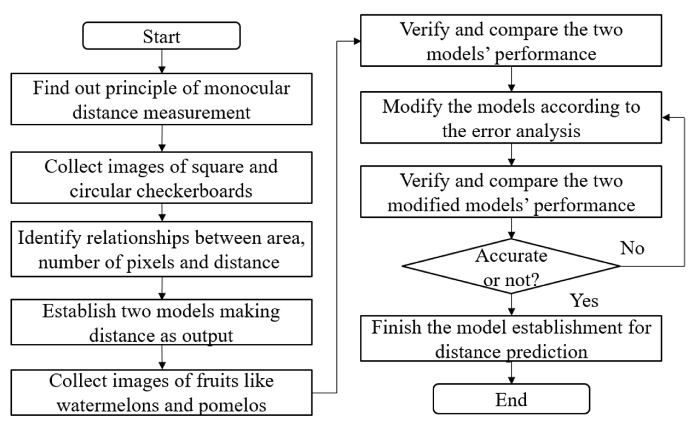
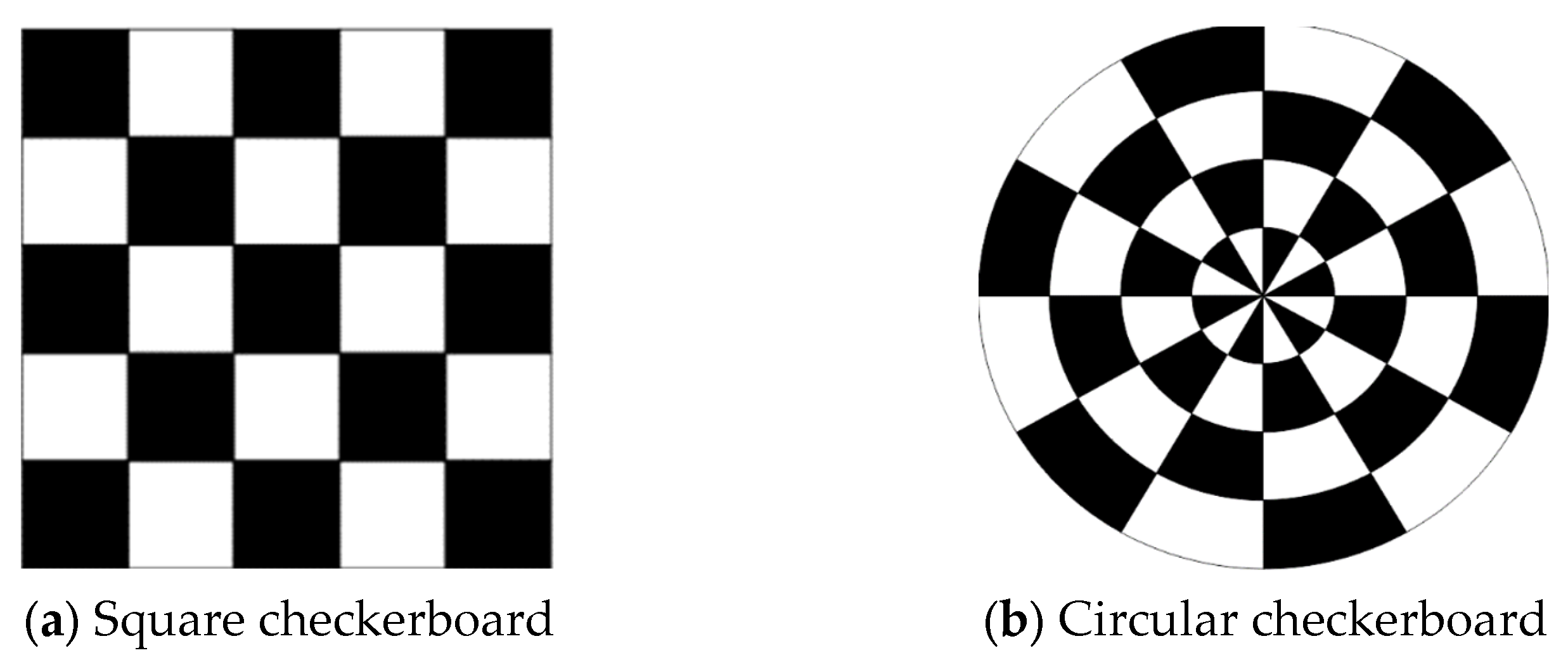
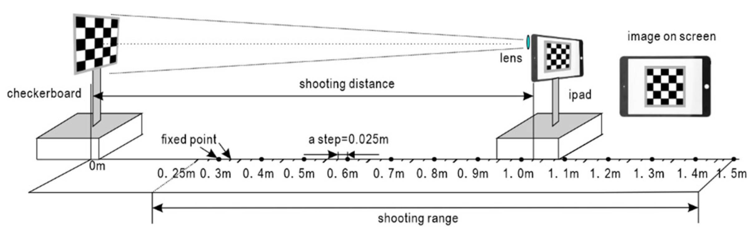
2. Materials and Methods

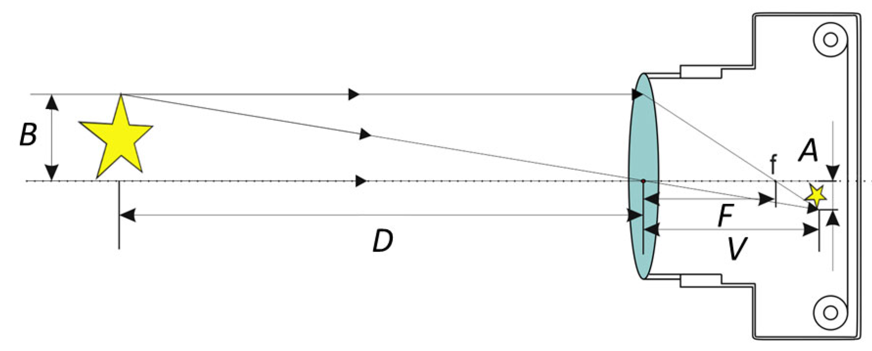
2.1. Principle of Monocular Distance Measurement

The monocular distance measurement was mainly achieved depending on all captured information from images collected by the camera. The principle of camera shooting was presented in Figure 2. The reflected light from the photographed subject was concentrated by the camera lens to form a real image in an area between one and two times the focal length from the optical center. When the shooting distance D was far greater than the focal length F, approximately the image distance would be seen as equal to the focal length.
1 F = 1 D + 1 V
Among those, V—image distance, D—the shooting distance, and F—the focal length.
Figure 2. Principle of camera shooting.
Horticulturae 09 00537 g002
According to the lens imaging principle and the principle of a similar triangle, it could be:
A F = B   D
A was the size of the real image formed in the camera, and B was the size of the shot object.
It is proposed that there are two patterns with the same area: a square of length L and a circle of radius R. As a result, the area S of the two patterns would be expressed as follows:
S = L 2 = π R 2
S represented the area, L represented the length of the square, and R represented the radius of the circle.
According to Equations (2) and (3), when a camera takes images of two patterns right from the front, the imaging areas would be expressed as:
s = F 2 D 2 · S
where s was the area of the real image formed in the camera.
On account of the shooting principle of the camera, the real image could be deemed an orderly array of pixels on the camera screen through the photoelectric converter and processor. Supposing the number of pixels of the video in the camera was x, the following equation described the special link between the imaging area of the objective and the number of pixels:
x = ω s
where ω represents a constant decided by the camera, x was the number of pixels of the image in the photo.
Therefore, conversion from number of pixels to distance was performed with the following simplification of the formula. There was a specific relationship between distance, number of pixels in the image, and area of the image:
D = β S x
where β was a constant collectively composed by F, S, and ω .

2.2. Model Establishment

The maximum projected area of large fruits such as pomelo and even larger fruits would range from 100 cm2 to 324 cm2 since the pomelo longitudinal axis length ranged over 100~170 mm mostly. Therefore, the square and circular checkerboard calibration plates, such as those in Figure 3, with the areas of 100 cm2, 121 cm2, 144 cm2, 169 cm2, 196 cm2, 225 cm2, 256 cm2, 289 cm2, and 324 cm2 as 9 groups were assigned and prepared for the establishment of models.
Under the condition that there was no sight line blocking within a certain positive range, as shown in Figure 4. The checkerboard was fixed, ensuring the checkerboard plane was perpendicular to the horizontal plane. For each checkerboard, 51 images were shot in the distance range from 0.25 m to 1.5 m at an interval of 0.025 m. Totally, 51 images shot from identical checkerboards were set as one group.
The number of pixels in the target image was calculated by Photoshop’s lasso tool. Then the information about square checkerboards and circular checkerboards (distance, area, and number of pixels) was loaded into MATLAB for two specific models whose formations were similar to Equation (6). The specification of the computer used was a LAPTOP-5V7TD45J with a CPU of AMD Ryzen 5 3500U with Radeon Vega Mobile Gfx (2.10 GHz).
In addition, to verify and polish the models, watermelon, and pomelo, two of the typical large-sized fruit, were selected to collect the image data under the same conditions. 12 groups of images were gathered together, involving 4 oval watermelons, 4 pyriform pomelos, and 4 oblate pomelos.
Each sample was assigned to pick four sides out for testing at an interval of 90°, as shown in Figure 5. The number of pixels and distance were recorded automatically. However, due to the irregular fruit’s outline, the maximum projected area of the fruit target could not be measured directly. Therefore, an estimation approach to the area was applied, considering there was an obvious linear relationship between area and number of pixels, in particular when the camera was far enough away. For square checkerboards and circular checkerboards, the relationships between the number of pixels and the grid area were shown in Figure 6, respectively, which could acquire estimated areas of the fruit. Further, all the results of the maximum projected area of samples calculated by two different methods are listed in Table 1. The predicted distance could be obtained when the number of pixels and the projected area of fruits were input into the models.
In this work, the accuracy of the model was classified into 3 grades to define the precise degree of prediction according to the number of relative errors—less than 5% relative error was assessed as “High” accuracy, between 5% and 10% was regarded as “Middle” accuracy, and higher than 10% was rated as “Low” accuracy. The model’s exact predicting ability would be justified by counting up the number of every grade. Furthermore, the maximum relative error and absolute error of the two prediction models were also essential parameters for evaluating the superiority of the models.

2.3. Model Error Modification

Considering the shape of the fruit is always irregular, errors in predicting results are inevitable. A modification for that, as an essential method, could effectively enhance the accuracy of a model. After the specific change tendency between the relative error and real distance was analyzed, a new modification polynomial was obtained. Via modification, the accuracy of models would be compared and evaluated again to observe the change.

3. Results and Discussion

3.1. Establishment of Models

According to the 18 groups of image data of the checkerboards with two shapes, a scatter diagram—Figure 7a—belonged to Model S, which described vividly specific distribution conditions in a three-dimensional coordinate system where the x axis, y axis, and z axis represented respectively the number of pixels, area of the checkerboard, and shooting distance. The curve-fitting surface of Figure 7b, whose distance starts at 0.25 m and culminates at 1.50 m in a three-dimensional coordinate, was obtained. The two functional relationships between Model S and Model C were:
d s = 22.64 S 0.4936 x 0.4932
and
d c = 23.51 S 0.4949 x 0.4990
ds and dc, respectively, represented the predicting distances of models S and C; S was the maximum projected area of the fruit sample, and x was the number of pixels in the image of the fruit sample. Table 2 lists the number of pixels and the image distance of a square-shaped checkerboard and a circular-shaped checkerboard with a 225 cm2 area.
Figure 7. The functional relationship between the area, number of pixels, and distance, including (a) the scatter point diagrams of Model S and (b) the curve surfaces from the scatter diagram fitting of Model S.
Horticulturae 09 00537 g007
After the models S and C were established, tests were designed to verify the accuracy of the model predictions. Two watermelons, two pyriform pomelos, and two oblate pomelos were picked, and each one gave four different aspects for camera shooting. The maximum projected area would be calculated through the linear relationship between the number of pixels and the area of checkerboards described in Figure 4. Hence, the predicting distance could be obtained when the maximum projected area and number of pixels are known inputs to models. The following Table 3 is an illustration of predicting results when one of the aspects of a watermelon was 110.72 cm2 in area.
The comparison of average absolute error, absolute error maximum, average relative error, and relative error maximum was exhibited in Table 4. It showed that model C had more priorities over model S for whatever shape: model C had a prominent advantage over accuracy with a 42 average number of “High” accuracy compared with model S at 35; while, for “Middle” and “Low” accuracy, model S obviously had more shares, taking account of an average of 8.75 and 7.25. Hence, it could be concluded that model C had more accuracy in predicting the imaging distance of the watermelon and pomelo targets.

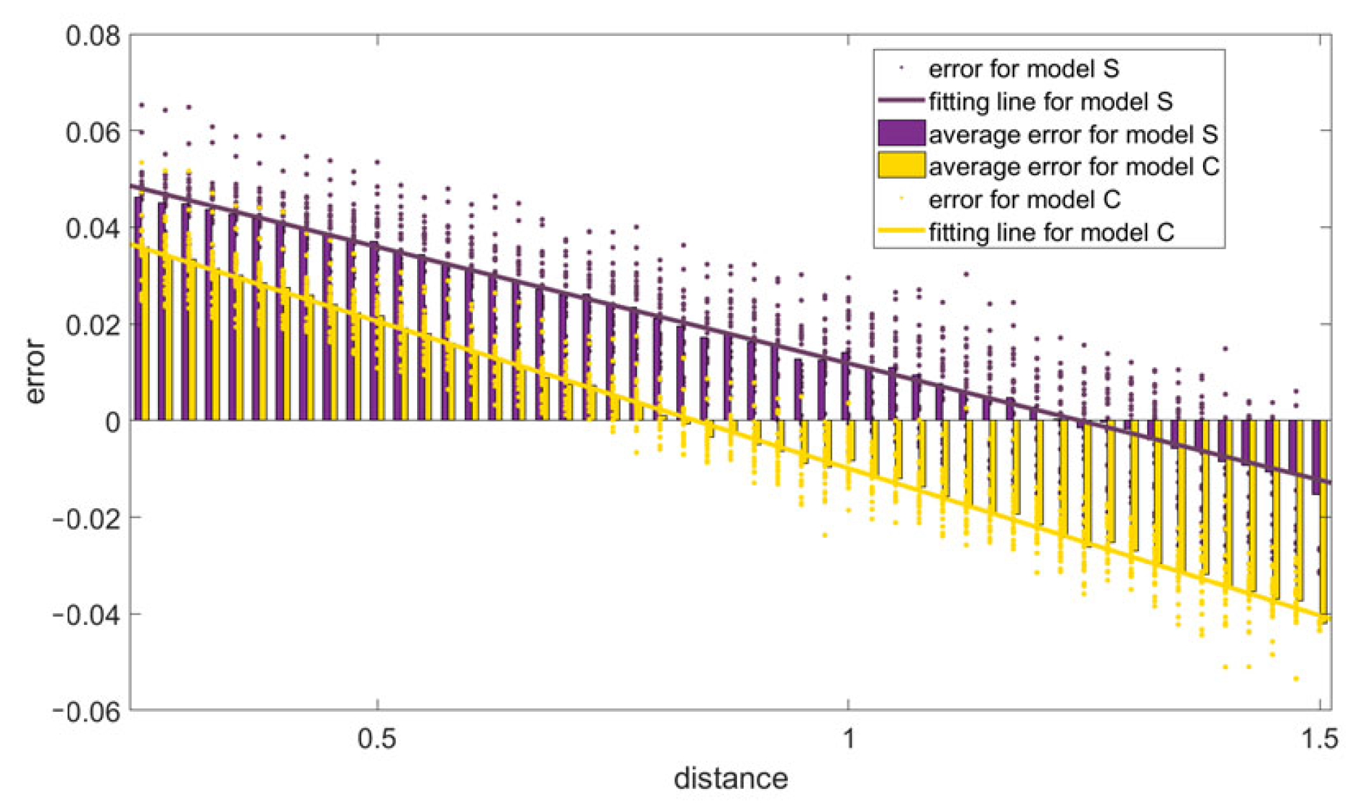
3.2. Model Modification

The detailed distribution of the predicted results was described in Figure 8, illustrating that the results would fluctuate around the ideal conditions with an error gap. In Figure 9, Range 1, Range 2, and Range 3 were respectively defined as the distance range where the predicting results could not be kept within [−10%,10%], the distance range where the predicting results could be kept within [−10%,10%] but some were over 5%, and the distance range where the predicting results can be curbed within [−5%,5%]. Based on Figure 9, which illustrated the conditions of relative error, three ranges, including Range 1 (0.25~0.525 m), Range 2 (0.525~0.8 m), and Range 3 (0.8~1.5 m), were divided. When shooting distance falls in Range 1, the results could not remain reliable; if in Range 2, the results could get an accuracy assurance within −10~10% error; if in Range 3, then the results would be accurate with only −5~5% error. Hence, when the distance is between 0.8 m and 1.5 m, it would make a sound effect; if the distance falls between 0.8 m and 1.5 m, there is a large improvement room to be more accurate for prediction.
According to Figure 10, where the fitting lines of two models were illustrated, the predicted error value changed step by step from negative to positive when the distance slowly decreased from 1.5 m to 0.25 m. Such a rough tendency for error fluctuation would be regarded as a ground for modifying the form of models. Namely, an approximately linear relationship would exist between real distance and predicting distance for two models. Via repeated fittings, two functional expressions could be described as:
d ps = 0.95274 d rs + 0.06
and
d pc = 0.93912 d rc + 0.05
dps and dpc represented predicting distance for model S and model C, and drs and drc represented real distance for model S and model C.
Figure 10. Distribution position of predicting distance error of model S and model C around distance, where the bars represent the average error at every distance.
Horticulturae 09 00537 g010
Substituting the above Equations (9) and (10) into Equations (7) and (8) and modifying models, respectively, could be:
d s = 23.83 S 0.4936 x 0.4932 0.063
and
d c = 25.01 S 0.4949 x 0.499 0.054
A comprehensive analysis, referring to several potential factors for predicting results, including average absolute error, absolute error maximum, average relative error, and relative error maximum, as well as accuracy shares, was carried out. From Table 5 and Figure 11, a clear improvement in accuracy for prediction could be seen after a simple modification. On the one hand, the number of “High” rating shares had a huge increase from 68.63% to 98.04% for Model S and from 82.35% to 98.53% for Model C. It meant almost all prediction results had less than 5% absolute error. On the other hand, the extinction of “Low” rating shares dropped significantly from 14.21% to 0 for Model S and from 6.73.% to 0 for Model C. Compared with model S, model C still retained a comprehensive edge in accuracy, with a higher average number of “High” classes and a lower absolute error maximum. Via modification, two methods had made the “High” accuracy rate increase to more than 98%.
The error of this model is mainly derived from two factors. The first one was the irregularity of pomelo and watermelon, which have an essential difference between an absolute square shape and a circle shape. Hence, the error was unavoidable in predicting the results. Another one was the transformation of the shoot side at different distances for even the same pomelo or watermelon fruit, due to the fact that when the camera is close to the fruit, the shoot side always tends to be smaller in view of the fruit as a three-dimensional object.

4. Conclusions

In this work, distance detection models based on the images of square checkerboards and circular checkerboards from only one camera were established, respectively. Two models described the special relationships among the three main imaging factors—shooting distance, the maximum projected area of the target, and number of pixels. The accuracy was tested on 2 oblate pomelos, 2 pyriform pomelos, and 2 oval watermelons. After error analysis, two models were modified and tested again. The main conclusions were as follows:
(1)
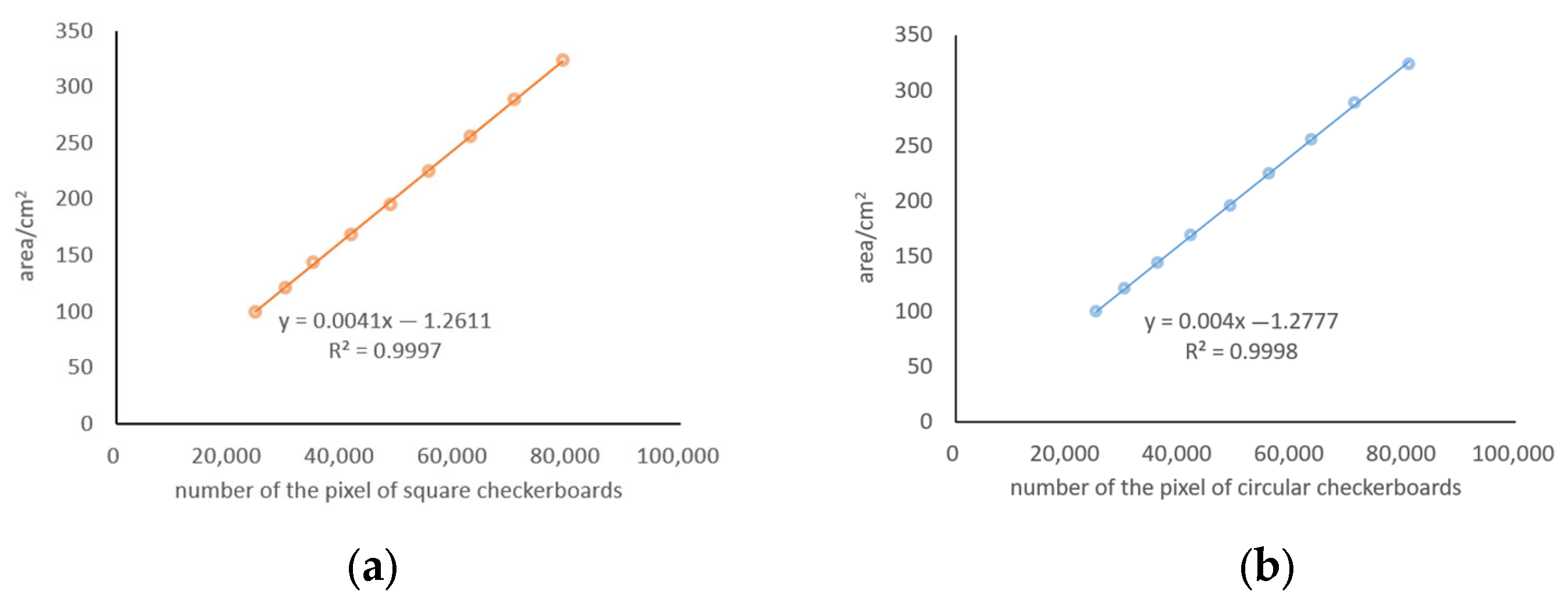
The regression model based on a square-shaped checkerboard could be presented as Equation (7), while a circular-shaped checkerboard could be presented as Equation (8).
(2)
According to the error analysis, two models were modified to Equations (11) and (12).
(3)
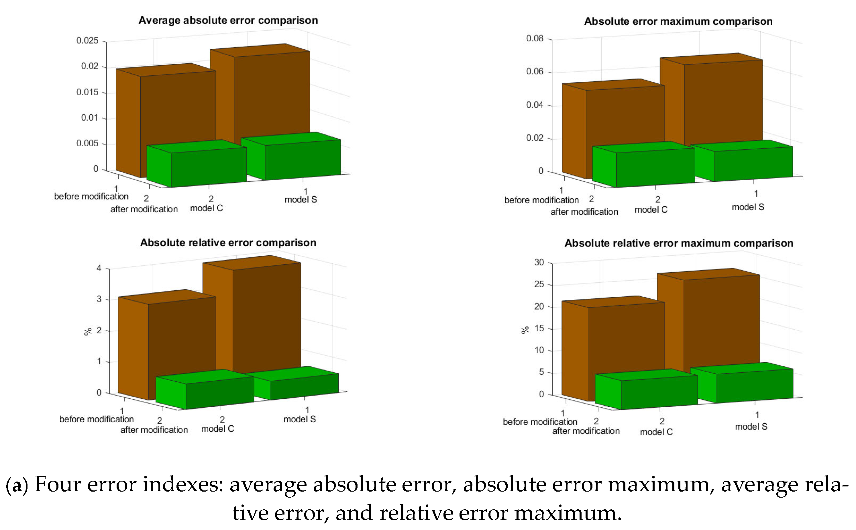
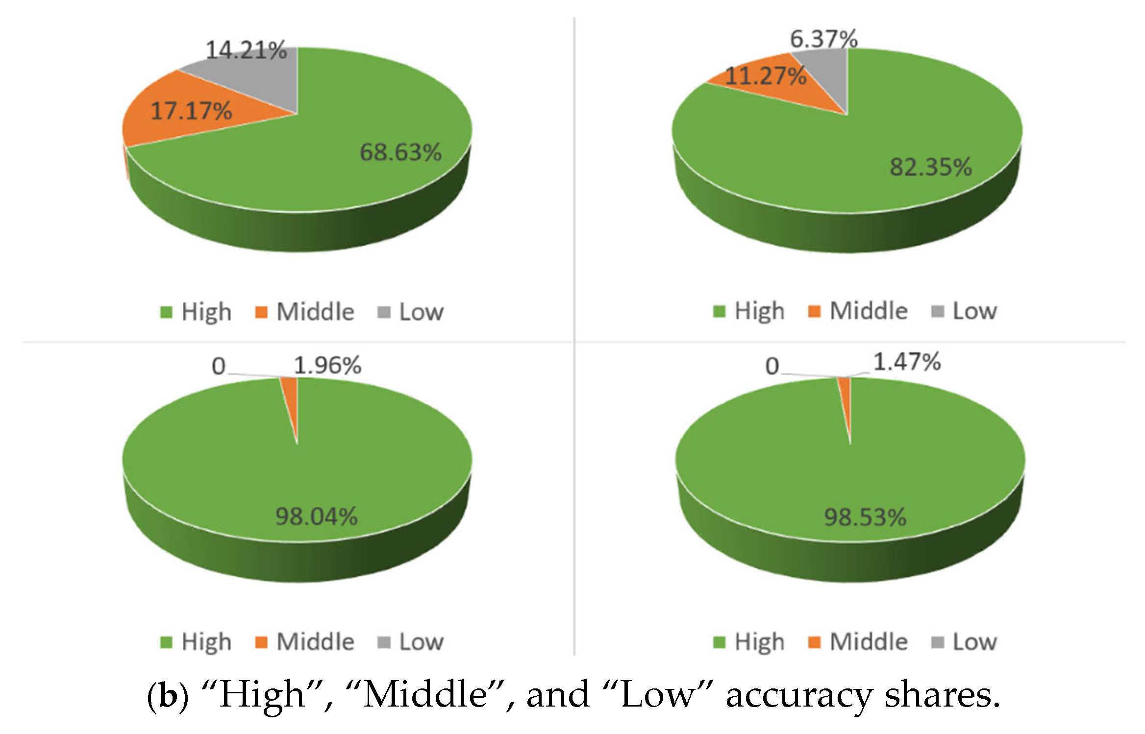
Two models had over 98% “high” accuracy and no “low” accuracy. By comparison, the model of a circular checkerboard would be more predictively accurate than the one of a square checkerboard when they were used for large fruits.
(4)
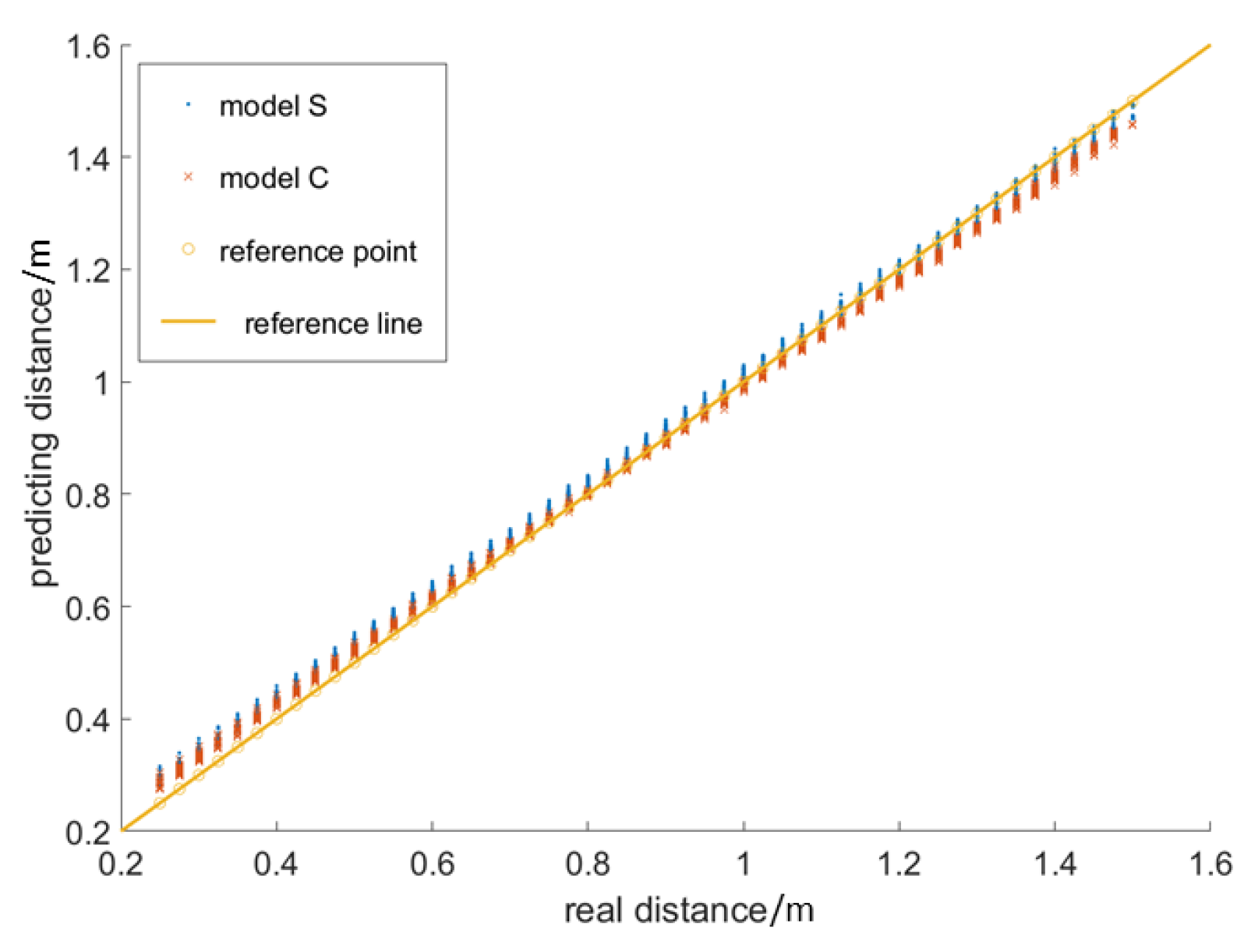
Two models showed a sound-predicting effect with a 0.8~1.5 m distance where the camera was far away shooting an object when applied to the watermelon and pomelo fruit, due to the relative error being controlled within 2%.
The results indicated that the proposed method provided a new way to achieve accurate distance measurement for fruit-picking devices. However, there would be some problems to overcome and deserve exploration in the future, such as the definite application and operation of that, the spreading of effective range, and further improvement of accuracy.

Author Contributions

Conceptualization, D.Z. and J.L.; formal analysis, D.Z., Y.L. and Y.W.; funding acquisition, J.L.; methodology, D.Z. and J.L.; project administration, J.L.; software, D.Z.; supervision, J.L.; validation, D.Z., Y.L., Y.W. and W.L.; visualization, D.Z.; writing—original draft, D.Z.; writing—review and editing, J.L. All authors have read and agreed to the published version of the manuscript.

Funding

The authors appreciate the support from the Fundamental Research Funds for the Central University [2662020GXPY011], the China Agriculture (Citrus) Research System [CARS-27], and the College of Engineering in the HZAU 2018 Subject Construction Funds [52904—108011807].

Institutional Review Board Statement

Not applicable.

Informed Consent Statement

Not applicable.

Data Availability Statement

Not applicable.

Conflicts of Interest

The authors declare no conflict of interest.

References

  1. Kang, D.; Chen, Z.J.; Fan, Y.H.; Li, C.; Mi, C.; Tang, Y.H. Optimization on kinematic characteristics and lightweight of a camellia fruit picking machine based on the kriging surrogate model. Mech. Ind. 2021, 22, 16. [Google Scholar] [CrossRef]
  2. Cao, X.; Yan, H.; Huang, Z.; Ai, S.; Xu, Y.; Fu, R.; Zou, X. A multi-objective particle swarm optimization for trajectory planning of fruit picking manipulator. Agronomy 2021, 11, 2286. [Google Scholar] [CrossRef]
  3. Pan, S.; Ahamed, T. Pear Recognition in an Orchard from 3D stereo camera datasets to develop a fruit picking mechanism using mask R-CNN. Sensors 2022, 22, 4187. [Google Scholar] [CrossRef] [PubMed]
  4. Rehman, A.; Saba, T.; Kashif, M.; Fati, S.M.; Bahaj, S.A.; Chaudhry, H. A revisit of Internet of Things technologies for monitoring and control strategies in smart agriculture. Agronomy 2022, 12, 127. [Google Scholar] [CrossRef]
  5. Kang, H.W.; Chen, C. Fruit Detection and Segmentation for Apple Harvesting Using Visual Sensor in Orchards. Sensors 2019, 19, 4599. [Google Scholar] [CrossRef] [PubMed]
  6. Zhang, F.; Chen, Z.; Wang, Y.; Bao, R.; Chen, X.; Fu, S.; Tian, M.; Zhang, Y. Research on flexible end-effectors with humanoid grasp function for small spherical fruit picking. Agriculture 2023, 13, 123. [Google Scholar] [CrossRef]
  7. Shi, Y.; Zhang, W. A “global-local” visual servo system for picking manipulators. Sensors 2020, 20, 3366. [Google Scholar] [CrossRef] [PubMed]
  8. Han, Y.; Routray, A.; Adeghate, J.O.; MacLachlan, R.A.; Martel, J.N.; Riviere, C.N. Monocular vision-based retinal membrane peeling with a handheld robot. ASME J. Med. Devices 2021, 15, 031014. [Google Scholar] [CrossRef] [PubMed]
  9. Fonder, M.; Ernst, D.; Van Droogenbroeck, M. M4depth: A motion-based approach for monocular depth estimation on video sequences. arXiv 2021, arXiv:2105.09847. [Google Scholar] [CrossRef]
  10. Tao, Y.; Zhou, J. Automatic apple recognition based on the fusion of color and 3D feature for robotic fruit picking. Comput. Electron. Agric. 2017, 142, 388–396. [Google Scholar] [CrossRef]
  11. Xiong, J.; Lin, R. The recognition of litchi clusters and the calculation of picking point in a nocturnal natural environment. Biosyst. Eng. 2018, 166, 44–57. [Google Scholar] [CrossRef]
  12. Wang, C.; Li, Z. Weed recognition using SVM model with fusion height and monocular image features. Trans. Chin. Soc. Agric. Eng. 2016, 32, 165–174. [Google Scholar]
  13. Liu, X.; Chen, S.W. Monocular camera based fruit counting and mapping with semantic data association. IEEE Robot. Autom. Lett. 2019, 4, 2296–2303. [Google Scholar] [CrossRef]
  14. Roberts, L. Machine Perception of Three-Dimensional Solids. Ph.D. Thesis, Massachusetts Institute of Technology, Cambridge, MA, USA, 1963. [Google Scholar]
  15. Yamaguti, N.; Oe, S. A method of distance measurement by using monocular camera. In Proceedings of the 36th SICE Annual Conference, International Session Papers, Tokushima, Japan, 29–31 July 1997; pp. 1255–1260. [Google Scholar]
  16. Kim, H.; Lin, C.S. Distance measurement using a single camera with a rotating mirror. Int. J. Control. Autom. 2005, 3, 542–551. [Google Scholar]
  17. Alizadeh, P.; Zeinali, M. A real-time object distance measurement using a monocular camera. In Proceedings of the Iasted International Conference on Modelling Simulation & Optimatization, Banff, AB, Canada, 1 January 2013; pp. 237–242. [Google Scholar]
  18. Xiao, D.; Zhai, J. Target distance measurement method with monocular vision for wheeled mobile robot. Comput. Eng. 2017, 43, 287–291. [Google Scholar]
  19. Huang, L.; Chen, Y. Measurement the absolute distance of a front vehicle from an in-car camera based on monocular vision and instance segmentation. J. Electron. Imaging 2018, 27, 043019.1–043019.10. [Google Scholar] [CrossRef]
  20. Bazrafkan, S.; Javidnia, H. Semiparallel deep neural network hybrid architecture: First application on depth from monocular camera. J. Electron. Imaging 2018, 27, 19. [Google Scholar] [CrossRef]
  21. Wang, X.; Zhou, B. Recognition and distance estimation of an irregular object in package sorting line based on monocular vision. Int. J. Adv. Robot. Syst. 2019, 16, 1729881419827215. [Google Scholar] [CrossRef]
  22. Bianco, S.; Buzzelli, M. A unifying representation for pixel-precise distance estimation. Multimed. Tools Appl. 2019, 78, 13767–13786. [Google Scholar] [CrossRef]
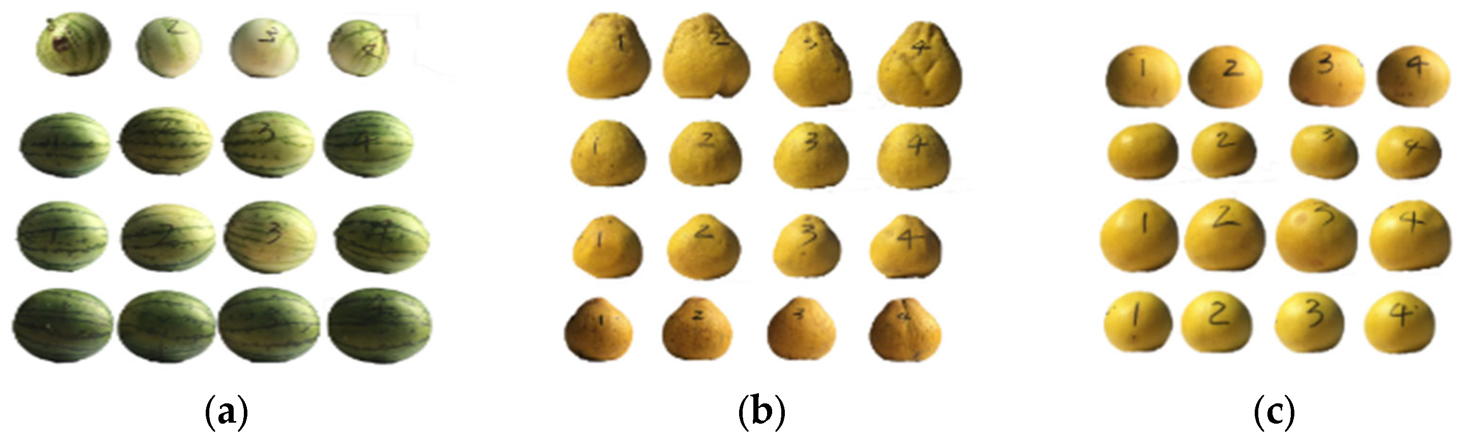
Figure 1. The flowchart of the main work.
Horticulturae 09 00537 g001
Figure 3. Two patterns of the checkerboard.
Horticulturae 09 00537 g003
Figure 4. The shooting device and the site environment for shooting.
Horticulturae 09 00537 g004
Figure 5. All samples of large fruits and their own 4 test sides: (a) oval watermelons; (b) pyriform pomelos; (c) oblate pomelos.
Horticulturae 09 00537 g005
Figure 6. The linear relationships between number of pixels and the area of checkerboards included (a) square and (b) circular.
Horticulturae 09 00537 g006
Figure 8. A series of points in a cartesian plane coordinate system with real distance as a horizontal axis and predicting distance as vertical coordinates for two models where the reference point and reference line are ideal goals.
Horticulturae 09 00537 g008
Figure 9. Distribution position of relative predicting distance error of model S and model C around distance, the average relative error, which are represented by bars at every distance.
Horticulturae 09 00537 g009
Figure 11. The compared results before and after modification.
Horticulturae 09 00537 g011aHorticulturae 09 00537 g011b
Table 1. The information was calculated by the area and number of pixels of sample fruit—type, shape, and number—as well as the maximum projected area of the four test sides obtained.
FruitShapeSample
Number
Maximum Projected Area/cm2
1st Side2nd Side3rd Side4th Side
SquareCircularSquareCircularSquareCircularSquareCircular
WatermelonOval1110.72107.97100.1097.61105.47102.8598.0995.65
WatermelonOval2145.98142.37153.09149.31150.29146.58150.17146.46
WatermelonOval3176.27171.93166.29162.18178.96174.55168.04163.89
WatermelonOval4206.83201.74201.52196.56209.09203.94204.83199.79
PomeloPyriform1172.54168.29178.82174.41169.55165.37176.97172.61
PomeloPyriform2124.06120.99125.84122.73124.74121.65126.37123.24
PomeloPyriform3101.3098.78103.65101.07102.74100.19102.98100.42
PomeloPyriform4128.40125.22128.75125.56124.32121.23125.19125.19
PomeloOblate179.1977.2176.3574.4477.7275.7876.2274.31
PomeloOblate2137.68134.28129.98126.76136.33132.96129.16125.96
PomeloOblate3133.42130.12139.58136.13136.81133.42139.71136.26
PomeloOblate4125.22123.48125.56123.79121.23118.95125.19122.68
Table 2. The number of pixels and shooting distance of 225 cm2 square checkerboard and circular checkerboard.
Distance (d)/mNumber of Pixels (x)Distance (d)/mNumber of Pixels (x)
Square
Checkerboard
Circular CheckerboardSquare
Checkerboard
Circular Checkerboard
0.2502,125,4002,027,9780.900157,169152,677
0.2751,810,9361,662,1040.925145,664144,729
0.3001,458,8581,386,5200.950137,918138,808
0.3251,277,8781,199,5610.975133,377131,268
0.3501,044,9691,018,6851.000125,000124,805
0.375941,468888,4871.025118,917119,939
0.400799,591776,8531.050112,923112,443
0.425721,767688,2631.075108,788108,577
0.450628,723619,1311.100102,864104,056
0.475575,948555,0151.12597,70699,427
0.500502,876500,6981.15093,54495,202
0.525471,042454,4381.17590,27890,870
0.550413,690414,6061.20086,20086,456
0.575385,746377,2841.22583,07484,213
0.600346,711347,1651.25079,72176,901
0.625325,720322,8231.27577,67574,469
0.650294,896297,6771.30073,68673,686
0.675275,735274,9911.32571,47171,481
0.700254,463253,4681.35068,58669,220
0.725239,976235,5871.37565,71966,114
0.750221,816221,4101.40062,92664,467
0.775209,194206,8591.42561,69061,875
0.800193,000194,5181.45058,61459,503
0.825183,087183,0711.47556,67357,292
0.850170,805172,7361.50055,23055,939
0.875163,039164,536
Table 3. Testing results for model S and model C with the watermelon of 110.72 cm2 maximum projected area.
d/mModel SModel Cd/mModel SModel C
dps/meas/mers/%dpc/meac/merc/%dps/meas/mers/%dpc/meac/merc/%
0.2500.2870.037514.9940.2760.026210.4970.9000.9120.0121.2890.8870.0131.435
0.2750.3140.03914.2140.3020.0279.8530.9250.9440.0192.0130.9190.0060.694
0.3000.3380.03812.5250.3250.0258.3150.9500.9670.0171.8340.9420.0080.840
0.3250.3610.03611.1560.3480.0237.0760.9750.9890.0141.4360.9630.0121.205
0.3500.3830.0339.4810.3690.0195.5311.0001.0150.0151.4710.9890.0111.142
0.3750.4110.0369.5690.3960.0215.6961.0251.0410.0161.5741.0150.0101.015
0.4000.4350.0358.7420.4200.0204.9641.0501.0630.0131.2771.0370.0131.281
0.4250.4610.0368.3710.4450.0204.6711.0751.0890.0141.2841.0620.0131.249
0.4500.4830.0337.4080.4670.0173.7961.1001.1120.0121.0731.0840.0161.432
0.4750.5060.0316.4450.4890.0142.9161.1251.1400.0151.3481.1120.0131.136
0.5000.5280.0285.6260.5110.0112.1721.1501.1590.0090.8161.1310.0191.638
0.5250.5530.0285.3260.5350.0101.9331.1751.1830.0080.6951.1550.0201.734
0.5500.5780.0285.0480.5590.0091.7131.2001.2130.0131.0771.1840.0161.334
0.5750.6000.0254.3900.5810.0061.1191.2251.2340.0090.7421.2050.0201.642
0.6000.6240.0243.9370.6040.0040.7221.2001.2560.0060.5151.2270.0231.845
0.6250.6480.0233.6790.6280.0030.5141.2751.2840.0090.6851.2540.0211.656
0.6500.6730.0233.6010.6530.0030.4811.3001.3080.0080.6161.2780.0221.703
0.6750.6980.0233.4450.6770.0020.3701.3251.3290.0040.2901.2980.0272.005
0.7000.7220.0223.1960.7010.0010.1651.3501.3510.0010.1071.3210.0292.165
0.7250.7490.0243.2470.7270.0020.2531.3751.3780.0030.1951.3470.0282.059
0.7500.7700.0202.6330.7480.0020.3121.4001.4150.0151.0611.3830.0171.183
0.7750.7910.0162.0410.7680.0070.8581.4251.4230.0020.1661.3910.0342.378
0.8000.8170.0172.1190.7940.0060.7471.4501.4440.0060.4171.4120.0382.607
0.8250.8410.0161.9830.8180.0070.8471.4751.4710.0040.2721.4390.0362.445
0.8500.8650.0151.7980.8420.0080.9971.5001.4900.0100.6401.4580.0422.790
0.8750.8910.0161.8350.8670.0080.929
Note: d—distance; S—the maximum projected area; dps, dpc—predicting distance of square model and circular model; eas, eac—absolute error of two models; ers, erc—relative error of two models.
Table 4. The error extremums and accuracy levels of two models.
FruitModel SModel C
Average
Absolute Error/m
Absolute Error Maximum/mAverage Relative Error/%Relative Error Maximum/%Average
Absolute Error/m
Absolute Error Maximum/mAverage
Relative Error/%
Relative Error Maximum/%
W10.0240.0654.37026.1100.0200.0533.21621.355
W20.0220.0484.16719.0810.0200.0483.02214.337
OP10.0170.0372.08014.5570.0180.0432.57411.614
OP20.0200.0513.28220.2760.0190.0423.11716.997
PP10.0270.0604.99123.8550.0200.0473.38018.930
PP20.0230.0514.36020.4830.0200.0423.17115.778
RH68.63%82.35%
RM17.17%11.27%
RL14.21%6.37%
Note: W1—watermelon NO.1, W2—watermelon NO.2; OP1—oblate pomelo NO.1, OP2—oblate pomelo NO.2; PP1—pyriform pomelo NO.1, PP2—pyriform pomelo NO.2. RH—rate of “High” accuracy; RM—rate of “Middle” accuracy; RL—rate of “Low” accuracy.
Table 5. The error extremums of the modified models.
FruitModel SModel C
Average
Absolute Error
Absolute
Error
Maximum
Average
Relative Error%
Relative Error
Maximum%
Average
Absolute Error
Absolute
Error
Maximum
Average
Relative
Error%
Relative
Error
Maximum%
W30.0090.0180.9294.5190.0050.0130.8094.625
W40.0120.0201.1836.6090.0070.0180.8116.622
OP30.0030.0110.2764.2390.0030.0120.8183.772
OP40.0070.0240.6812.5910.0030.0120.8212.399
PP30.0040.0150.3873.7670.0030.0120.8263.425
PP40.0060.0180.6104.1660.0070.0210.8303.850
RH98.04%98.53%
RM1.96%1.47%
RL00
Note: W3—watermelon NO.3, W4—watermelon NO.4; OP3—oblate pomelo NO.3, OP4—oblate pomelo NO.4; PP3—pyriform pomelo NO.3, PP4—pyriform pomelo NO.4. RH—rate of “High” accuracy; RM—rate of “Middle” accuracy; RL—rate of “Low” accuracy.
Disclaimer/Publisher’s Note: The statements, opinions and data contained in all publications are solely those of the individual author(s) and contributor(s) and not of MDPI and/or the editor(s). MDPI and/or the editor(s) disclaim responsibility for any injury to people or property resulting from any ideas, methods, instructions or products referred to in the content.

