Article

Relieving the Phenotyping Bottleneck for Grape Bunch Architecture in Grapevine Breeding Research: Implementation of a 3D-Based Phenotyping Approach for Quantitative Trait Locus Mapping

1
Federal Research Centre for Cultivated Plants, Julius Kühn-Institut (JKI), Institute for Grapevine Breeding Geilweilerhof, 76833 Siebeldingen, Germany
2
Institute of Crop Science and Resource Conservation (INRES)–Plant Breeding, Katzenburgweg 5, 53113 Bonn, Germany
3
Institute for Computer Science 4, University of Bonn, Friedrich-Hirzebruch-Allee 5, 53115 Bonn, Germany
*
Author to whom correspondence should be addressed.
Horticulturae 2022, 8(10), 907; https://doi.org/10.3390/horticulturae8100907
Submission received: 11 September 2022 / Revised: 26 September 2022 / Accepted: 27 September 2022 / Published: 5 October 2022
(This article belongs to the Section Viticulture)

Abstract

:
In viticulture, winemakers and the industry demand grape bunches that have a reduced degree of bunch compactness. The major aspect is that a loose bunch compactness reduces the risk of severe Botrytis bunch-rot infections. Grapevine breeders focus hereby on several bunch-architecture-related traits. For specific breeding approaches and breeding-research-related topics, such as Quantitative Trait Locus (QTL) analysis or molecular marker development, the exact and objective phenotyping of such traits is mandatory. In this study, a precise and high-throughput 3D phenotyping pipeline was applied to screen 1514 genotypes from three mapping populations with different genetic backgrounds to investigate its applicability for QTL mapping approaches. In the first step, the phenotypic data of one population containing 150 genotypes were collected and analyzed with the 3D phenotyping pipeline. Additionally, corresponding reference data were obtained. Phenotypic values and results of a QTL analysis were compared with each other. Strongly positive correlations up to r = 0.93 between 3D and reference measurements could be detected for several traits. The ten-times-faster 3D phenotyping pipeline revealed 20, and the reference phenotyping methods revealed 22 QTLs. Eighteen of these QTLs were consistent between both procedures. In the next step, screening was extended to four different mapping populations across several seasons. In total, up to 1500 genotypes were screened during one season (>5000 grape bunches in total). The data analysis revealed significant differences across years and populations. Three bunch-architecture traits, including total berry volume, bunch width, and berry diameter, explained the highest amount of variability in the phenotypic data. A QTL analysis was performed on the phenotypic data of the involved populations to identify comparative genetic loci for bunch-architecture traits. Between 20 and 26 stable and reproducible QTLs for the investigated populations were detected. A common QTL for berry diameter could be identified for all populations. Our results strongly conclude that this locus is co-located on chromosome 17 when mapped to the grapevine reference genome. The results show that the implementation of the 3D phenotyping platform allows for precise and extended screenings of different, genetic diverse mapping populations and thus opens up the possibility to uncover the genomic architecture of this highly complex quantitative grapevine trait.

1. Introduction

The selection of grapevine (Vitis vinifera ssp. vinifera L.) clones and breeding material that express a loose grape-bunch architecture is one of the major goals in wine- and table-grape breeding [1,2,3]. Multiple studies have shown a close link between a compact, dense bunch architecture and a higher susceptibility against the bunch-rot-inducing fungal pathogen Botrytis cinerea (Botrytis) [4,5]. The Botrytis infection, causing gray mold or Botrytis bunch rot, has a high potential of triggering economical damage due to a reduction of yield and wine quality, especially if humid weather conditions occur during bloom and/or harvest time [6,7]. In consequence, controlling Botrytis bunch rot (and other pathogens) requires intense viticultural management procedures such as defoliation and plant protection [7,8]. Besides the compactness of grapes, smaller berries were recently associated with a reduction in the risk for Botrytis bunch rot [5]. However, for Botrytis, no reports on mapping successful defense-related genes are available yet. Therefore, alternative strategies are applied in breeding programs [9,10]. Breeders hereby mainly focus on a loose bunch architecture to strengthen the resilience of grape berries against Botrytis bunch rot [2,3,11]. Besides these phytosanitary aspects, a loose grape bunch architecture is additionally associated with positive effects on the berry ripening rate and berry compositions (see the detailed overview of Tello and Ibanez, 2018 [7]). The compactness of a grape bunch depends strongly on the synergy of two structure-defining traits: (1) berry characteristics, i.e., berry number and size; and (2) stem-related traits, i.e., rachis length, pedicel length, and width of the grape bunch [9,12,13]. The degree of bunch compactness is, thus, determined by the interaction of individual bunch-architecture-related traits.
The phenotyping of bunch architecture is mostly performed in the field and focuses commonly on the visual rating of grape-bunch density. The International Organization of Vine and Wine (OIV) published an optical descriptor for bunch density (OIV descriptor 204) [14]. This five-class system rates bunches according to the degree of compactness, from a very loose (class 1) to a very dense (class 9) structure [14]. In general, such classification data have several restrictions, as they are determined by subjectivity and are rather superficial, as they do not give any detailed information on the single traits/characteristics that affect bunch compactness [15,16,17]. Increasing the degree of detail and measuring the sub-traits is laborious and expensive, as it requires trained employees. This often limits the number of assessed samples per season and is recognized as the phenotypic bottleneck [18]. Several studies showed the potential of two-dimensional (2D)-based or three-dimensional (3D)-based sensor technologies to overcome the phenotyping bottleneck for grape-bunch-architecture-related traits [17,19,20]. As a result, a substantially increased number of phenotypic samples, together with a high precision of numeric data, are required to characterize single or multiple grape-bunch architecture-related traits. Sensor technologies open the possibility for an effective and objective bunch-architecture screening of grapevine populations with subsequent QTL analyses. The QTL analysis is a powerful tool in breeding research to identify genetic regions contributing to the manifestation of a trait. Positional, closely linked markers can later be used for an extended marker-assisted selection (MAS) within early selection of breeding material [21,22]. In the last years, several studies have targeted bunch-architecture-related traits, gaining insights into the relationships between involved sub-traits and the underlying genetic architecture of grapevine, as well as table, grapes [23,24,25,26,27]. Fanizza et al. determined the grape bunch weight, the number of berries per bunch, and the berry weight within a table-grape population (‘Italia’ × ‘Big Perlon’) of 184 genotypes over three years [28]. The identified QTLs showed a high variability over the three consecutive seasons. For instance, for the traits berry number and berry weight, they could not find recurring regions. For bunch weight, however, they could identify one consistent QTL on chromosome 5. In addition, Correa et al. measured rachis length and used the weight of 50 berries to approximate the total number of berries of 137 genotypes of an experimental table-grape population of ‘Ruby Seedless’ × ‘Sultanina’ [26]. Their analysis revealed 19 QTLs distributed on chromosomes 5, 8, 9, 14, 17, and 18 for the examined traits. Most of the mentioned studies used labor-intensive manual low-throughput methods for phenotyping, resulting in a low number of replicates of the investigated plant material (less than 200 genotypes). So far, QTL mapping is mainly conducted within relatively small population sizes of less than 190 offspring individuals [21]. A high number of genotypes, together with dense marker information, are needed for the validation of QTL mapping results for complex traits that are highly affected by the environment. Therefore, an increased number of genotypes within populations and different independent mapping populations are required [21,28,29]. To meet these challenging demands, high-throughput phenotyping methods are crucial to overcome this bottleneck by a substantial increase of the sample size and to facilitate phenomic and genomic studies. Recently, only a few studies have applied sensor-based phenotypic data for genetic analyses, which are mostly based on 2D-imaging methods for grape-bunch phenotyping [20,23]. Richter et al. used RGB images to quantify berry-related traits (e.g., the total number of berries and rachis-related traits) [23]. The QTL analysis revealed about 30 QTLs with LODmax values of up to 11 explaining around 30% of phenotypic variation. On this basis, the applicability of a structured light-based 3D sensor was validated for grape-bunch phenotyping [13]. The scanning procedure mentioned in Rist et al. [13] does not require any invasive steps, thus resulting in an approximately ten-times-faster workflow in comparison to an automated image-based method [13]. In addition, an automated software framework was developed and can be used to analyze resulting 3D point clouds of whole grape bunches to extract all the individual traits needed for the phenotyping of grape-bunch architecture [13,17]: berry number, mean berry diameter and volume, total berry volume (total volume), bunch width, and bunch length. The testing panel included samples from four different grapevine cultivars, as well as a subset of 41 genotypes of the mapping population ‘Calardis Musqué’ (GF.GA-47-42) × ‘Villard Blanc’ (C × V) [13,30]. For the cultivar samples, a direct comparison of the 2D-related reference measurements with the 3D-related data revealed high correlation coefficients up to r = 0.93 for berry number and r = 0.83 for total volume [13].
Regarding the demand of high-throughput phenotyping methods, these novel tools must be applicable generally on highly diverse material with a broad genetic background. Furthermore, the sensor-based data should be usable for proper genetic analyses. The present study addresses three major aspects: (I) The reliability of the 3D-based phenotypic data in comparison to established 2D-based data was verified by phenotyping the core population of C × V (respectively six bunches each of 150 genotypes), using both methods. Furthermore, the phenotypic data recorded with both methods were applied for QTL mapping and identified QTLs were compared for validation. (II) The phenotyping and QTL analysis were expanded on three additional cross-populations (i.e., (1) an independently crossed C × V population with 722 genotypes, (2) a ‘Dakapo’ × ‘Cabernet Sauvignon’ population with 347 genotypes, and (III) a ‘Riesling’ × ‘Sauvignon Blanc’ cross with 295 genotypes) in order to identify transferable QTLs. (III) The physical positions of these QTLs on the Vitis vinifera reference genome PN40024 12X.v2 were compared to identify coherence and general determining factors that are transferable between divergent genetic backgrounds.

2. Materials and Methods

2.1. Plant Material

The study took place at the experimental vineyards at JKI Geilweilerhof (N49°13.070, E8°02.790) in Siebeldingen, under the cool climate conditions of Germany. Four F1 mapping populations were screened between 2016 and 2020.
(1) The grape bunches of 150 genotypes (n = 150) of the mapping population ‘Calardis Musqué’ VIVC4549 (‘Bacchus Weiß‘ VIVC851 × ‘Seyval Blanc‘ VIVC11558) × ‘Villard Blanc’ VIVC13081 (Seibel 6468 VIVC11181 × ‘Subereux‘ VIVC12031) (C × V_150) were investigated over three consecutive seasons in 2016, 2017, and 2018. This population was grafted on ‘SO4′ (VIVC11473) and planted in the year 2010 on two adjacent vineyards, with four replicates per genotype. (2) An extended population of C × V, derived from an independent C × V cross, planted in 2014 with approximately 1000 genotypes (C × V_1000), was screened in the season 2018. Almost 300 plants showed a reduced amount of fertility or less than three representative bunches and thus were not considered for this study. The remaining 722 genotypes (n = 722) were further analyzed. (3) A total of 347 genotypes (n = 347) from a cross of ‘Dakapo’ VIVC14728 (‘Deckrot’ VIVC3482 × ‘Portugieser Blau’ VIVC9620) × ‘Cabernet Sauvignon’ VIVC1929 (‘Cabernet Franc’ VIVC1927 × ‘Sauvignon Blanc’ VIVC10790) (D × C) that was planted in 2015 were phenotyped from 2018 to 2020. (4) A total of 295 genotypes (n = 295) of a ‘Riesling Weiß’ VIVC10077 (Unknown × ‘Heunisch Weiß’ VIVC5374) × ‘Sauvignon Blanc’ VIVC10790 (‘Traminer’ VIVC17636 × Unknown) (R × S) cross, also planted in 2015, were phenotyped from 2018 to 2020.
Except for the C × V_150 population, the other populations were not grafted and planted in a slope direction. All investigated populations were trained in a vertical shoot positioning (VSP) trellis system (10 to 12 buds), with a plant density of 5000 vines per hectare (2 × 1 m spacing). Treatment was applied according to local best-practice policies for viticulture.

2.2. Sampling

In this study, the sampling of grape bunches was standardized over the investigated populations. Six bunches per genotype for the C × V_150 population (three representative bunches from each genotype per vineyard) and three grape bunches per genotype for the other populations were used for this study (for instance, 4992 bunches from 1514 genotypes in 2018). The samples were taken from the basal insertion of the first three central shoots of the fruit cane. All bunches were cut directly at their connection with the shoots when they reached the developmental stage of maturity (BBCH 89) [31]. Until further proceedings, all grape bunches were stored at 4 °C (maximum of one week).

2.3. Three-Dimensional Data Acquisition and Analysis

The 3D data acquisition followed the established procedure, as described in detail by Rist et al. and Mack et al. [13,32]. The bunches were fixed on a motorized hook, rotating with 0.5 s−1 or 0.16 s−1 (depending on sample size and shape) in order to take 360° scans of the bunches. The 3D scanner Artec Spider (Artec 3D, L-1466, Luxembourg) was used to scan the complete structure of bunches. The scanning distance varied between 25 and 30 cm (in adjustment to sample size and shape). After the scanning process, point clouds of the samples were saved in polygon file format. In the laboratory, a standard ceiling illumination was used. Point cloud analysis was performed with the ‘3D Bunch Tool’. The algorithm analyzes segments and characterizes the point clouds in spherical regions (see Rist et al. and Mack et al. [13,32] for a more detailed description of the procedure). Subsequently, several important phenotypic parameters are extracted: the number of berries (BN), mean berry diameter (Dia), mean berry volume (BV), total (berry) volume (TV), convex hull volume (CVH), bunch width (W), and bunch length (L).

2.4. Two-Dimensional and Manual Data Acquisition

In order to compare the 3D phenotypic data to already established measurement methods based on 2D Red–Green–Blue (RGB) images, extended reference measurements were taken for the grapes of C × V_150. These manual measurements were taken in the course of the work of Richter et al. [23]. For referencing the 3D-based phenotypic data, the 2D ‘Berry Analysis Tool’ (BAT) was used. Therefore, all berries of individual bunches had to be removed and placed on a perforated plate. Under standardized light conditions, a picture was captured and subsequently analyzed with BAT [33]. With this tool, the following traits can be acquired: the total number of berries per bunch (ref_BN), the single berry diameter (ref_Dia) and volume (ref_BV), and the total berry volume (ref_TV). After removing the berries, an image of the rachis, together with a size standard, was taken. The rachis (Rac) and pedicel length (Ped) were measured with the ImageJ tool, according to Richter et al. [23]. The manually measured bunch volume (MBV) was deduced by placing them in polyethylene bags, removing the air and submerging the bunches in a container of water (according to Ferreira et al. [34]). The weight of the individual bunches was measured manually on a digital scale. Then the compactness of all bunches was rated according to the OIV 204 (OIV204) optical descriptor for bunch density (class 1: very loose structure; class 9: very dense structure) [14]. Manual measurements in 2017 and 2018 were reduced to manual weight measurements. For R × S, D × C and C × V_1000, only 3D-based measurements were conducted.

2.5. Applied Genetic Maps

The integrated genetic maps used in this study were developed by using the multipoint maximum likelihood method in JoinMap® Version 4.1 software and resulted in 19 chromosomes (numbered and oriented) according to the PN40024 reference genome [35]. The map of C × V_150 is a revised version of the map published by Zyprian et al. [30], with 150 individuals and 394 SSR markers, a total size of 1621 centimorgan (cM), and 4.1 cM average distance between markers. The map of C × V_1000 consists of data of 995 individuals of the extended population. The map is based on 210 SSR markers and has a total length of 1396 cM and an average distance between markers of 6.6 cM (Schwandner et al. unpublished). The DxC map includes 739 individuals evaluated with 270 SSR markers. This resulted in a total map length of 1500 cM, with an average marker distance of 5.5 cM (Schwander et al. unpublished). The RxC map consists of 285 SSR markers applied on 716 individuals, has a total length of 1592 cM, and an average marker distance of 5.6 cM (Schwander et al. unpublished).

2.6. QTL Analysis

For the population C × V_150, R × S, and D × C, phenotypic data of three years were recorded. QTL analyses were performed separately for every single season (year). QTLs that occurred in at least two of the three seasons were considered as reproducible. In such cases, QTLs were calculated with three-year mean values for each of the sub-traits additionally. For C × V_1000, only one-year data were available (2018) and used for the QTL analysis. The resulting QTLs of this population were considered to be preliminary QTLs.
MapQTL6.0 [36] was used for the calculation of QTLs of all the measured phenotypic traits. Interval mapping (IM) with one cM step size was performed. A permutation test with 1000 iterations (p < 0.05) was conducted to determine a chromosome-specific trait-linked “logarithm of the odds” (LOD) threshold. QTL regions were defined as genetic regions that exceed this calculated LOD threshold. For each QTL, the percentage of explained phenotypic variance and the maximum LOD score (LODmax) and its genetic position (LODmax position) were listed. In the case that a direct LODmax linked marker was available, this marker name is additionally listed (Supplementary Tables S1 and S2).

2.7. Statistical Analysis

For validation of the 3D-derived phenotypic data, a direct comparison to all measured 2D image data, the manually measured grape-bunch parameter MBV, and the OIV 204 factor was performed by correlation analysis (α = 0.05). Furthermore, direct correlation analyses between TV and the manual bunch weight were performed on the data of 2016, 2017, and 2018. An analysis of variance (ANOVA) was further used to compare 2D vs. 3D measurement methods (α = 0.05). The results of the QTL analysis from 3D- and 2D-image-related data, i.e., berry number (BN), bunch length vs. rachis (L), berry diameter (Dia), berry volume (BV), and total volume (TV), were compared to each other. LODmax values, LODmax position, and the QTL intervals of the matching QTL regions were evaluated by a correlation analysis and comparison of mean values (for both, α = 0.05) (Supplementary Figures S2 and S3).
An ANOVA was further performed on the phenotypic data of the different populations to compare variability of seasons, as well as between populations (in this case, three-year mean values were used) (Supplementary Figures S4–S6). Subsequently, phenotypic data from all populations were used for a principal component analysis (PCA). All statistical analyses were performed with R version 3.5.2 [37]. The emmeans package [38] was used for all ANOVA-based analyses. The ggplot2 [39], ggpubr [40], corrplot [41], and factoextra packages [42] were used to create the visualizations.

2.8. Approximation of Physical QTL Positions

In order to find general QTL regions for bunch-architecture traits among the investigated populations, the QTL positions were compared. The genetic maps that were used in this study differ to a certain degree between populations concerning the mapped markers and the marker saturation, making a direct comparison of QTL positions difficult. Thus, the positions of the most proximal QTL flanking markers were transferred on the grapevine reference genome PN40024 12X v2 [43] and further compared. The region was determined by the flanking markers of the genetic region, limited by the chromosome-specific LOD threshold (confidence interval).

3. Results

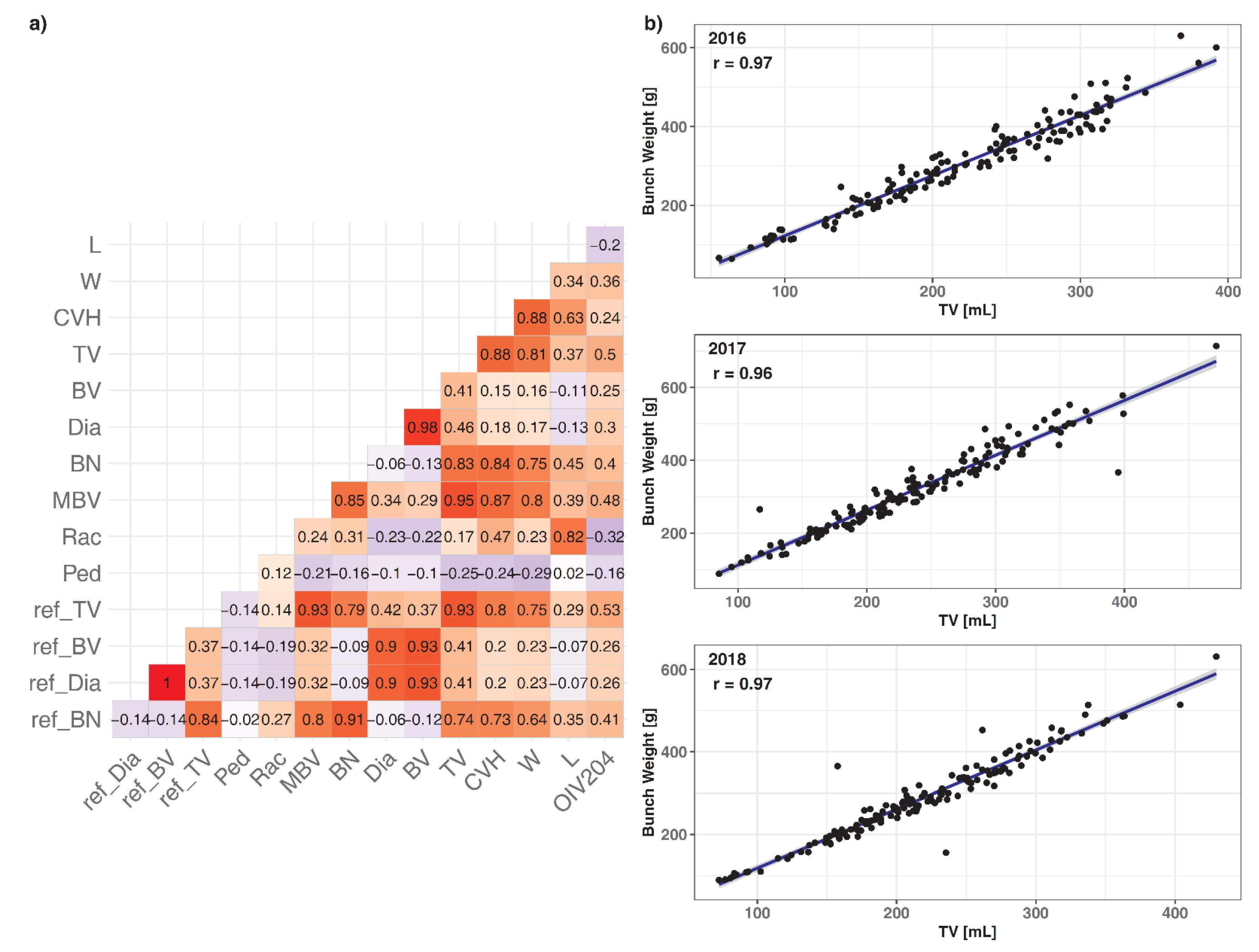
3.1. Direct Comparison between 3D, 2D, and Manually Measured Data of 150 Genotypes

To validate the reliability of 3D-based phenotypic data, in the first step, the 3D-based phenotypic data were correlated with the 2D and manual measurement data of all 150 individuals of the C × V_150 population.
The correlation analysis between 3D and 2D phenotypic values showed correlations ranging between r = 0.93 and r = 0.82 for the related traits (Figure 1a). The 2D data of the pedicel length (Ped) had no respective 3D measured data for a direct comparison. An indirect comparison with all other traits revealed only minor correlations (Figure 1a). The manually measured bunch volume (MBV) showed a high correlation coefficient with the TV and CVH (r = 0.95–0.87). The correlation of the phenotypic 3D data with the optical descriptor OIV204 showed, on average, a lower correlation in comparison to the comparable 2D data (Figure 1a). Furthermore, the correlations between manually measured bunch weight and TV showed very high values, ranging between r = 0.96 and r = 0.97, over the three consecutive seasons (Figure 1b). A direct comparison of the 3D vs. corresponding 2D phenotypic data revealed significant differences between BN, BV, and TV (Supplementary Figure S1). For the trait BV, the 3D data showed higher values in comparison to 2D measured values and lower value ranges for the trait BN (Supplementary Figure S1).

3.2. Comparison of Detected QTLs in CxV_150 Based on 3D and Corresponding 2D Data

After the correlation analysis, the data were used in a QTL mapping approach, and the results were compared to each other. The 3D phenotypic data revealed 20 QTLs, whereas the 2D phenotypic data resulted in 22 QTLs for bunch architecture, determining traits in CxV_150 and explaining a phenotypic variance between 8.7% and 16.8% for the 3D phenotypic trait data and between 8.1% and 17.1% for the 2D phenotypic data (Table 1 and Supplementary Table S1). The 3D data showed two unique QTLs for L and BV, and the 2D and manually measured data showed a unique QTL for BN, L, and BV (Table 1 and Supplementary Table S1).
Eighteen QTLs were matching between the two methods. Concerning these matching QTL regions, correlation coefficients between r = 0.78 and r = 0.97 could be observed for LODmax positions, LODmax values, and intervals of the matching QTLs (Supplementary Figure S2). Furthermore, no significant differences were observed for these parameters (Supplementary Figure S3).

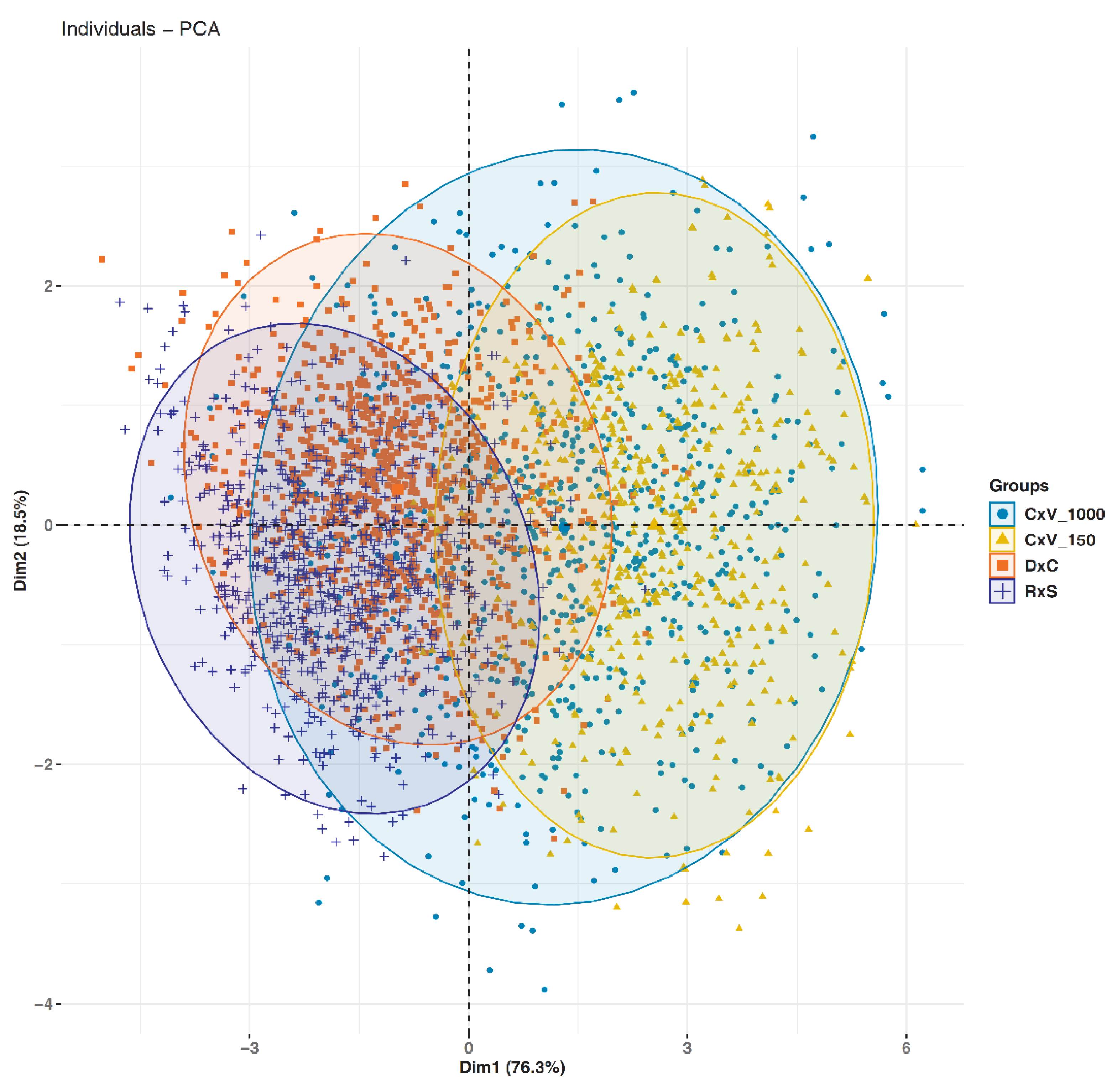
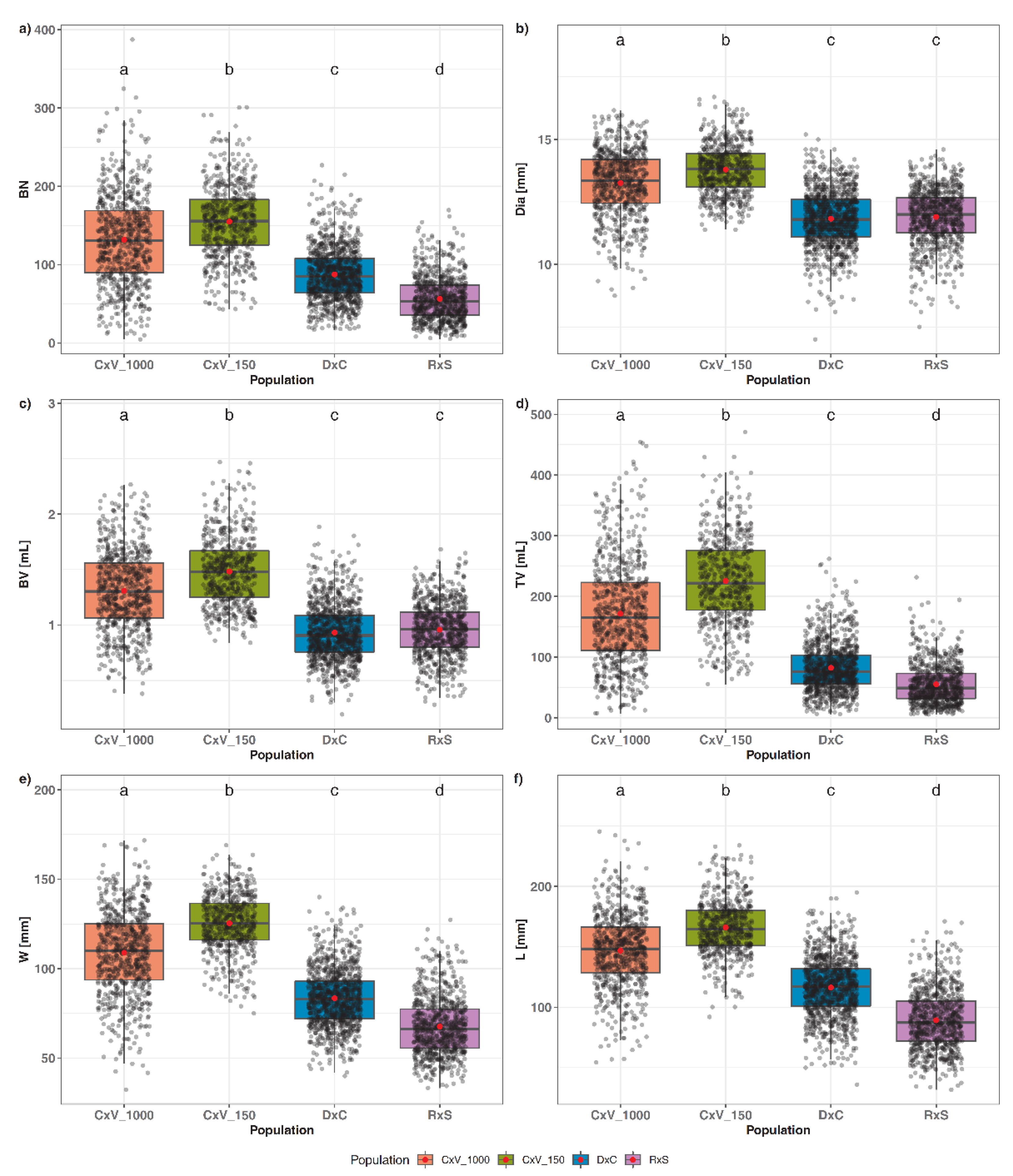
3.3. High-Throughput 3D Phenotyping of Different Populations

The 3D-phenotyping pipeline was applied in a breeding-research-related framework to test the practical implementation for high-throughput phenotyping. Therefore, different mapping populations were screened throughout various seasons. The comparison between the 3D data from three consecutive seasons of C × V_150, R × S, and D × C showed significant differences in at least two years for every investigated trait (Supplementary Figures S4–S6). In a next step, the phenotypic variation between the populations was investigated. For this analysis, data of C × V_1000 (derived from the season 2018) were included, and a PCA was performed on the phenotypic values. A moderate population-specific pattern was observed between C × V_150 and the two populations D × C and R × S (Figure 2). The C × V_1000 population spanned over all populations (Figure 2). Dimension 1 (Dim1) explained 76.3% of the total variance, with TV (20.5%), W (19.5%), L (17.3%), and BN (15.6%) as the main contributors. Dimension 2 (Dim2) explained 18.5% of the total variance, with BV (33.6%), Dia (32,9%), and BN (22.4%) as the main contributors.
An ANOVA was performed over the phenotypic values of the populations. Significant differences were found between all investigated populations (Figure 3). Highest phenotypic-value ranges for all investigated traits were observed for the C × V_150 population (Figure 3). R × S and D × C showed the lowest phenotypic-value ranges for the measured traits (Figure 3). For both populations, the traits Dia and BV showed no significant differences (Figure 3b,c).

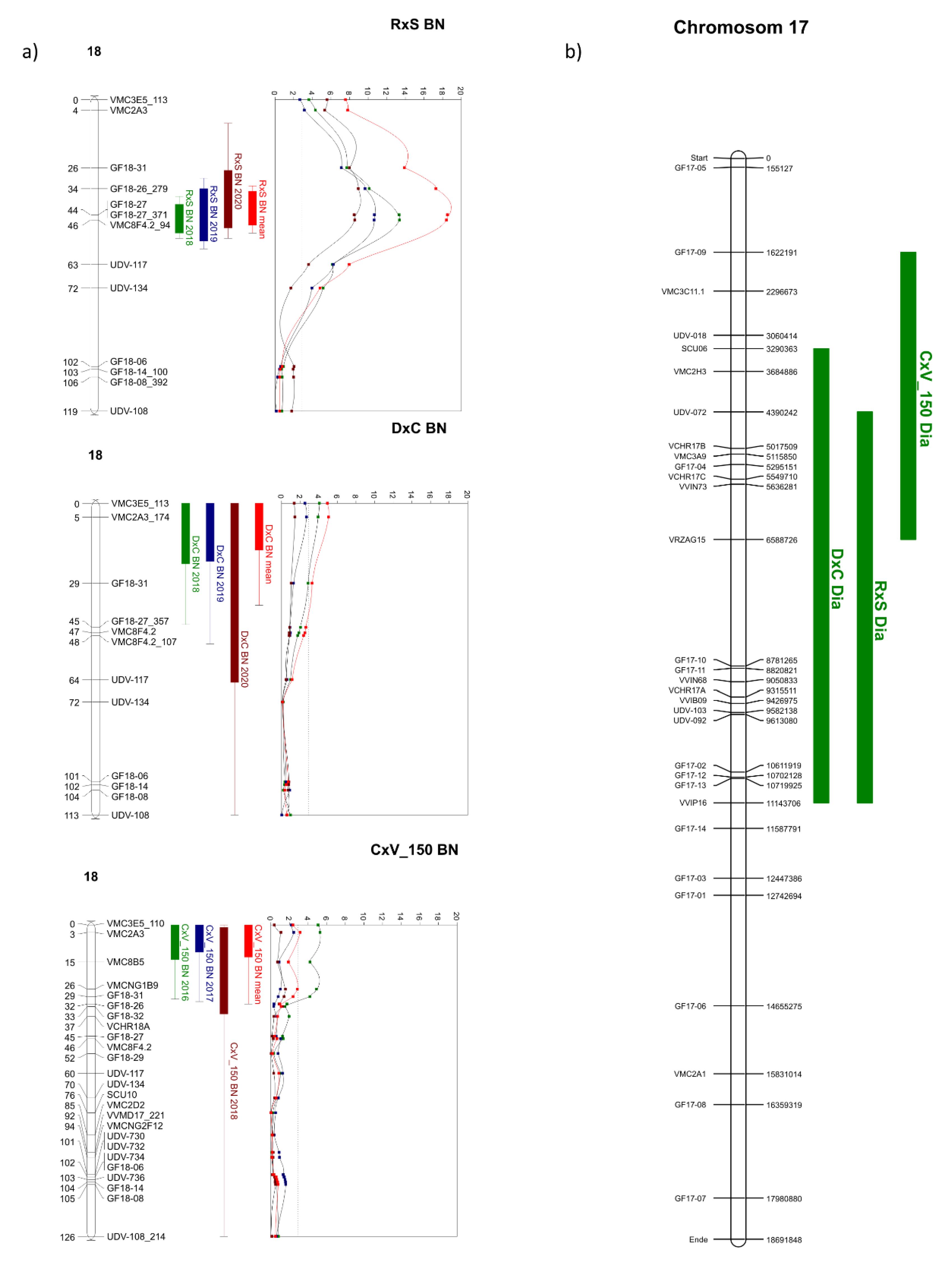
3.4. QTL Analysis for the Investigated Populations

A QTL analysis was conducted with the phenotypic data recorded across all seasons and for each population. Seasonal differences could be observed between the populations (data not shown). For the sake of simplicity, only the LOD curves/preliminary QTL for the trait BN on chromosome 18 are reported as an example. On this chromosome, Richter et al. found a QTL for BN in C × V_150 [23]. For our experiments, C × V_150 and D × C showed a putative QTL with significant LOD values in one season, whereas R × S showed a QTL occurring in all three recorded seasons (Figure 4a and Supplementary Table S2). To reduce seasonal uncertainty and to streamline the analysis, further QTLs were calculated by using phenotypic mean values from the traits that show significant LOD values in at least two seasons. The resulting QTLs were considered to be reproducible (Supplementary Table S2). Here, C × V_150 showed 26 QTLs, D × C showed 20 QTLs, and R × S showed 20 QTLs in total (Supplementary Table S2). Table 2 lists only QTLs that occur in at least two populations on the same chromosome. In total, 31 reproducible QTLs with LODmax values up to 20.06 distributed over 12 chromosomes could be detected for the populations R × S, D × C, and C × V_150. Out of the 29 QTLs, only the QTL for Dia occurred in all populations on the same chromosome, whereas 11 QTLs occurred in two populations (note that only multiyear QTLs are considered). Additionally, to validate the results of the C × V_150 population, preliminary QTLs from the 2018 data of the extended population C × V_1000 were also included for a direct comparison between these two populations (Table 2). Between both populations, 15 QTLs/preliminary QTLs were identified on the same chromosomes (Table 2). Note that the preliminary QTLs of C × V_1000 were excluded from this point on.
The positions of the QTLs for Dia observed in all three populations (highlighted in Table 2) were then further investigated. The physical positions of mapped linked markers in the reference genome PN40024 12X.v2 were used to approximate the physical positions of the QTLs (preliminary QTLs of C × V_1000 were not considered). The linked marker of all three QTLs for Dia on chromosome 17 from the investigated populations were co-localized on the reference genome PN40024 12X.v2 (Figure 4b).

4. Discussion

In this study, an automated 3D-based phenotyping pipeline was applied for screening multiple mapping populations and tested for its feasibility to study grape-bunch-architecture-determining traits for a high number of samples. The performance of the obtained 3D phenotypic data was assessed by three different approaches: (i) validation of the phenotypic precision of 3D sensor data by comparison to corresponding reference data within an entire mapping population; (ii) comparison of QTLs obtained from both 3D and reference phenotypic data; and (iii) screening and comparative QTL analysis with up to 1500 genotypes of several mapping populations for the assessment of seasonal effects and identification of general determining factors.

4.1. Three-Dimensional-Based Approach Enables Phenotypic Studies with High Throughput and Precision

The 3D-based phenotyping has been proven to be a reliable method for the modern plant phenotyping of many different species [44]. The data gathered from 3D sensors can be used to measure plant and fruit parameters with high accuracies and correlations in comparison to ground-truth data [45,46,47,48]. For grape-bunch-related 3D phenotyping, Tello et al. compared bunch-volume estimations derived from a 2D image analysis with 3D scan data of grape bunches. Both methods reached correlations of approximately r = 0.95 in comparison to ground-truth measurements [49]. Hacking et al. scanned 21 grape bunches in the lab and compared 2D-image- and 3D-scan-derived bunch weight with actual bunch weight [50]. They obtained correlations of r2 = 0.89 and 0.95 for the 2D-based and 3D-based data, respectively. Those results are in accordance with the correlations between 3D, 2D, and manual volume measurements observed in this study. A subset of the data, recorded in 2016, was already used for referencing the proposed 3D phenotyping method [13]. It is notable that this subset only represented a fraction of the phenotypic highly diverse mapping population C × V_150 [13,17,23]. The reference data set that was used within this study includes the whole mapping population of 150 genotypes (i.e., 900 grape bunches or six bunches per genotype). Despite the strongly increased number of reference data, the high correlations reported in Rist et al. could be confirmed in this study [13]. Additionally, the field of application could be extended to the grape-bunch weight—one of the most important yield traits in viticulture [51]. Based on the observed very high correlation between the TV and grape-bunch weight (Figure 1), one can conclude that the 3D-based approach is also suitable for the proper estimation of this trait. In the present study, this comparison was additionally used as an indirect quality control for the 3D sensor data, as the TV is approximated by the total number of detected berries per bunch and their corresponding volumes. Taken together, the results verified the reliability of the 3D method for measuring bunch-architecture-determining traits.

4.2. Three-Dimensional vs. Two-Dimensional QTL Comparison

The detection of a QTL for a quantitative trait such as bunch architecture depends on several different factors. One factor is the range of phenotypic variability for the trait(s) of interest within the investigated population. For the C × V_150 population, a few studies already demonstrated this variability and segregation for several, traits including bunch-architecture-related traits [2,13,17,23,30,33]. In this study, the high correlation between 3D and reference data is also reflected in the results of the QTL-comparison. The 3D data revealed 20 QTLS, and the 2D data revealed 22 QTLs, with 18 consistent QTLs between the two investigated methods. It is noteworthy that the comparison between the 3D bunch length and measured 2D rachis length is indirect. In the 3D scans, the measured value is a product of the rachis itself, the number of berries attached to this structure, and the experimental procedure (bunch fixed on a hook). This differs from the 2D measurements of the rachis, where all berries had been removed, which also has an impact on shape. Nevertheless, the data revealed two consistent QTLs for both traits in CxV_150 (Table 1 and Supplementary Table S1). Although the phenotypic values were derived from slightly different measurement methods, they show a higher correlation (r = 0.82), and this might explain the concordance of QTLs for 3D-measured bunch length and 2D-measured bunch length. Regarding the outcome of the QTL analysis with 18 matching QTLs between the two methods, the 3D-data-derived LODmax values showed lower correlations and tended to have lower LODmax values in comparison to the reference data. The direct comparison of the ANOVA results of the phenotypic data also indicates this (Supplementary Figure S1). Here, the 3D data showed lower mean values for the majority of the compared phenotypic parameters. The results suggest that QTLs with lower LODmax values might not be detected by the 3D method. Correctional terms/models could be used to correct measurement uncertainties and prevent this loss of information. Future studies could address performance tests and validate potential correctional terms. Nevertheless, all the 18 matching QTLs found by 3D and 2D ground-truth measurements showed no greater difference in interval length and LODmax position (correlation of r = 0.97 and r = 0.96, respectively; see Supplementary Figure S2b,c). Regarding the amount of time that can be saved by applying this method and the mentioned results, the 3D phenotyping pipeline is highly valuable in the context of genetic investigations.

4.3. Sample Size of Investigated Populations

For genetic studies, one major restrictive factor is the number of samples that can be phenotyped by classical, often laborious, manual methods [18,52]. In this study, the application of the sensor overcame this phenotypic bottleneck, as it allowed for screenings of several populations of different sizes in one season, simultaneously, in a short amount of time and with a standardized procedure. In the season of 2018, the population C × V_150, with 150 individuals, was analyzed. This population is rather small, whereas the additionally screened mapping populations had a much higher number of genotypes, i.e., D × C (n = 342), R × S (n = 295), and the extended C × V_1000 population (n = 722). Thus, the number of screened genotypes add up to over 1500, and the screening rate could be improved by the factor of 10 in comparison to the 2D-based referencing methods used in this study [13,23,33]. One additional important advantage of the non-invasive 3D pipeline is the opportunity of subsequent investigations of, for example, phenotyping of the grape berry skin or conducting infection tests with Botrytis cinerea or insect pests such as Drosophila suzukii [5,53]. For both research topics, information about the grape-bunch architecture is essential, and intact, unharmed grapes and berries are needed. Focusing on the outcome of the QTL analyses, we can see that, for C × V_150 compared to C × V_1000, both populations result from independent crosses of the same parental varieties, and thus, they have the same genetic background. In C × V_1000, an approximately three-times-higher number of preliminary QTLs were detected, and the phenotypic variability that can be explained by a single one-year/preliminary QTL decreases by about 50% on average. There are different possible explanations for these results. On the one hand, both populations differ in age (C × V_150 planted in 2010; C × V_1000 in 2014), which might have an impact in phenotypic expression of the measured parameter. In a recent study, it was shown for the grape variety ‘Zinfandel’ that age can have an impact on the timing of different phenological events [54]. The soil properties are different for both populations (C × V_150, clayey-loam soil with higher upper-soil moisture; C × V_1000, higher sand proportion and lower upper-soil moisture (data not shown)). Additionally, C × V_1000 was planted in the slope direction, and the genotypes were not grafted on a rootstock, whereas C × V_150 was grafted. These factors can have an impact on water and nutrient uptake, thus affecting bunch-architecture-related traits such as the berry number and berry size [7]. On the other hand, it is widely accepted that an increased numbers of genotypes can lead to an increase in statistical power of the QTL analysis. This sharpens the detection of a QTL and the estimation of its effect [55]. The comparison of the QTLs resulting from C × V_150 together with D × C and R × S supports this. Here, the populations showed a similar number of QTLs, but D × C and R × S showed higher LOD values for certain QTLs (e.g., BN and Dia). Additionally, a higher number of samples can reduce the number of false-positive QTLs [26,55,56]. The several preliminary QTLs from C × V_1000 that occur on the same chromosome as reliable three-year QTLs of C × V_150 are an indication of this. Multi-year phenotyping, mapping of additional molecular markers, and alignment of the genetic maps could improve the identification of reliable QTLs occurring both in C × V_150 and C × V_1000 and facilitate the comparison to other populations.
Further, QTL analyses should also consider environmental parameters such as soil properties and management, as both influence the phenotypic behavior of grape traits [57] (Bendel et al., in preparation).

4.4. Seasonal Effect

The sensor was applied on several populations over three seasons. This allowed the comparison of phenotypic variations over these years. All investigated populations showed differences in phenotypic data and in the outcome of the QTL results throughout the seasons. For bunch-architecture-related traits, it is widely recognized that the seasonal/environmental effect can be very strong (overview is given in References [58,59]). This results in phenotypic differences, the presence or absence of a QTL, and a certain amount of variability in the position of a QTL over the seasons [23]. The present study resulted in similar observations as those described in the literature. For instance, the trait berry number (BN) explained a major amount of measured phenotypic variance within the PCA analysis. The formation of berries per bunch underlies several complex processes. In temperate climates, these processes are extending over two consecutive seasons and are affected by the interaction of various environmental signals and gene networks from the formation of flowers to fruit set to the final number of berries per bunch [7,60,61,62]. This makes the detection of stable and reproducible genomic regions (QTLs or SNPs) affecting the trait difficult [28,60]. Exemplarily, this study focused on chromosome 18 and the resulting QTL for BN. In the populations C × V_150 and D × C, only a putative one-year QTL was observed, indicating a stronger environmental effect on this trait for both populations (Supplementary Table S2; Figure 4a). It is noteworthy that the QTL for BN on chromosome 18 in C × V_150, as reported in Richter et al. [23], could only be reproduced in the season of 2016. Additionally, no QTL for the BN in the season of 2018 for the extended C × V_1000 population could be detected [23]. This implies that the BN is under a much stronger environmental influence for C × V. On the other hand, the genetic map of C × V_150 used in this study differs from the map of Richter et al. [23]. A reanalysis of the phenotypic data with the same map version could bring further clarification on the stability of the mentioned QTL. On the contrary, for R × S, a promising QTL over all investigated seasons was detected. Our results suggest that there is a certain and detectable amount of environmental impact on these traits, but this impact is variety dependent [28]. Altogether, our results indicate that high-throughput screening allows us to identify and distinguish between populations that are under less environmental influence for such highly (environmentally) affected traits. Such knowledge can be further used in breeding to select appropriate breeding material for loose bunch architecture and to clarify further research questions. Furthermore, the effect of different environments on grape-bunch architecture can be investigated by such an objective sensor-based approach.

4.5. Comparison of QTL Positions

For the comparison of QTL positions, only one trait (Dia) revealed a QTL on the same chromosome among all populations. Our results show that all QTL intervals are co-located according to the physical mapping on the reference genome PN40024 on Chr. 17. Dia correlates strongly with BV and can be associated with berry size, which impacts the weight of the berries (Figure 1). It is apparent that berry-size/berry-weight-related traits were important selection targets during the domestication process [63]. Our results imply that this region might be conserved among different populations/and genetic backgrounds. Other studies also report about genomic regions associated with berry size. In the study of Doligez et al., for instance, QTLs for berry weight were identified in several grapevine mapping populations, as well as on chromosome 17 near the marker VVIN73 [64]. The group of Guo et al. performed a genome-wide association analysis on a diverse panel of 179 grapevine genotypes [65]. They identified an SNP on chromosome 17 related to berry weight. In recent years, several studies have identified meaningful QTL regions, SNP positions, and possible candidate genes that influence bunch-architecture-related traits [5,9,23,25,58,60,64,66]. The results in the present study and the findings of the mentioned studies indicate that genetic regions, affecting bunch-architecture-related traits, are conserved within a broader genetic background, and the proposed 3D phenotyping method is feasible for the rapid and precise screening of phenotypic material. The genetic maps of the investigated populations share the majority of markers, but they also (with a certain amount) have different mapped markers and differ in marker saturation. For some of the detected QTLs, this led to a difficult determination of the exact intervals. An aligned, denser, and more homogeneous marker saturation for the genetic maps of the investigated populations would increase the precision for the proposed QTL regions and improve the comparability of the QTLs in different populations. Another approach could be the use of these data in a meta-QTL analysis. Delfino et al. identified 17 meta-QTLs related to veraison on the basis of 43 different QTL studies [67]. Finally, fine mapping of promising genetic regions is necessary to identify candidate genes, as well as to develop a set of new molecular markers selecting for looser grape bunches and validate them by applying the 3D-based phenotyping method.

5. Conclusions

This study applied a novel 3D-based phenotyping pipeline for high-throughput phenotyping of bunch-architecture-related traits in different mapping populations for QTL analysis. Based on the 3D analysis of approximately 5000 different grape bunches, it was shown that this phenotyping pipeline is reliable to use for grapevine bunches in order to conduct phenotypic studies with high precision. The major benefit of this approach is the reduced amount of time that is needed to assess multiple phenotypic parameters in one simple working step, enabling phenotyping of a 10-times-increased sample size at the same time within one season and without long-term experience, as it is needed for visual scorings. The application of the sensor system on different mapping populations and subsequent QTL analysis led to comparable QTL regions that are associated with bunch-architecture-related traits. These results show the high-standard value of the novel sensor system for breeding/research purposes. The use of the sensor-based phenotyping pipeline over multiple years and multiple populations or genetic repositories all over the world would offer a much clearer picture of the genetic structure of bunch-architecture-related traits. Moreover, the combination of the phenotypic data with high-density genetic maps (e.g., SNP-based) and fitting the involvement of environmental parameter to the phenotypic behavior would enable much higher precision for determining genetic regions and, much more important, the identification and verification of promising candidate genes. This information could be used for further genetic analyses and the development of informative molecular markers, and it could therefore benefit breeders in order to select breeding material regarding, for example, loose bunch architecture.

Supplementary Materials

The following are available online at https://www.mdpi.com/article/10.3390/horticulturae8100907/s1. Figure S1: Analysis of Variance between 3D and 2D phenotypic reference data; Figure S2: Correlation analysis between the 2D/3D-matching QTLs; Figure S3: Comparison of the overlapping QTL regions; Figure S4: Analysis of variance between three-year phenotypic data of C × V_150; Figure S5: Analysis of variance between three-year phenotypic data of D × C; Figure S6: Analysis of variance between three-year phenotypic data of R × S; Table S1: Overview of QTLs derived from 3D and 2D (reference) phenotypic values from the corresponding traits of the Population C × V_150 in 2016; Table S2: Overview of reproducible QTLs derived from the phenotypic values from the corresponding traits of the consecutive seasons 2018-2020.

Author Contributions

Conceptualization, F.R., F.S. and K.H.; methodology, F.R. and F.S.; software, J.M. and V.S.; validation, F.R. and F.S.; formal analysis, F.R.; investigation, F.R.; resources, K.H. and R.T.; data curation, F.R.; writing—original draft preparation, F.R., F.S. and K.H.; writing—review and editing, K.H., F.S., R.T., R.R., A.S., L.H., V.S. and J.M.; visualization, F.R. and F.S.; supervision, K.H.; project administration, K.H. and R.T.; funding acquisition, R.T. and V.S. All authors have read and agreed to the published version of the manuscript.

Funding

This research was funded by the German Research Foundation (Deutsche Forschungsgemeinschaft (DFG), Bonn, Germany (Automated Evaluation and Comparison of Grapevine Genotypes by means of Grape Cluster Architecture, TO 152/6-1 and STE 806/2-1).

Data Availability Statement

Data available on request. The data presented in this study are available on request from the corresponding author.

Acknowledgments

We want to thank Patrick Römer and Margrit Daum (Julius Kühn-Institut, Institute for Grapevine Breeding Geilweilerhof) for their excellent technical support.

Conflicts of Interest

The authors declare no conflict of interest.

References

  1. Migicovsky, Z.; Sawler, J.; Gardner, K.M.; Aradhya, M.K.; Prins, B.H.; Schwaninger, H.R.; Bustamante, C.D.; Buckler, E.S.; Zhong, G.Y.; Brown, P.J.; et al. Patterns of Genomic and Phenomic Diversity in Wine and Table Grapes. Hortic. Res. 2017, 4, 1–11. [Google Scholar] [CrossRef] [PubMed] [Green Version]
  2. Herzog, K.; Wind, R.; Töpfer, R. Impedance of the Grape Berry Cuticle as a Novel Phenotypic Trait to Estimate Resistance to Botrytis Cinerea. Sensors 2015, 15, 12498–12512. [Google Scholar] [CrossRef] [PubMed]
  3. Tello, J.; Torres-Pérez, R.; Flutre, T.; Grimplet, J.; Ibáñez, J. VviUCC1 Nucleotide Diversity, Linkage Disequilibrium and Association with Rachis Architecture Traits in Grapevine. Genes 2020, 11, 598. [Google Scholar] [CrossRef]
  4. Molitor, D.; Behr, M.; Hoffmann, L.; Evers, D. Impact of Grape Cluster Division on Cluster Morphology and Bunch Rot Epidemic. Am. J. Enol. Vitic. 2012, 63, 508–514. [Google Scholar] [CrossRef]
  5. Herzog, K.; Schwander, F.; Kassemeyer, H.-H.; Bieler, E.; Dürrenberger, M.; Trapp, O.; Töpfer, R. Towards Sensor-Based Phenotyping of Physical Barriers of Grapes to Improve Resilience to Botrytis Bunch Rot. Front. Plant Sci. 2022, 12, 3299. [Google Scholar] [CrossRef] [PubMed]
  6. Dean, R.; Van Kan, J.A.L.; Pretorius, Z.A.; Hammond-Kosack, K.E.; Di Pietro, A.; Spanu, P.D.; Rudd, J.J.; Dickman, M.; Kahmann, R.; Ellis, J.; et al. The Top 10 Fungal Pathogens in Molecular Plant Pathology. Molecular plant pathology 2012, 13, 414–430. [Google Scholar] [CrossRef] [Green Version]
  7. Tello, J.; Ibáñez, J. What Do We Know about Grapevine Bunch Compactness? A State-of-the-Art Review. Aust. J. Grape Wine Res. 2018, 24, 6–23. [Google Scholar] [CrossRef]
  8. Pertot, I.; Caffi, T.; Rossi, V.; Mugnai, L.; Hoffmann, C.; Grando, M.S.; Gary, C.; Lafond, D.; Duso, C.; Thiery, D.; et al. A Critical Review of Plant Protection Tools for Reducing Pesticide Use on Grapevine and New Perspectives for the Implementation of IPM in Viticulture. Crop Prot. 2017, 97, 70–84. [Google Scholar] [CrossRef]
  9. Richter, R.; Rossmann, S.; Gabriel, D.; Töpfer, R.; Theres, K.; Zyprian, E. Differential Expression of Transcription Factor- and Further Growth-Related Genes Correlates with Contrasting Cluster Architecture in Vitis Vinifera ‘Pinot Noir’ and Vitis Spp. Genotypes. Theor. Appl. Genet. 2020, 1, 3. [Google Scholar] [CrossRef]
  10. Töpfer, R.; Hausmann, L.; Harst, M.; Maul, E.; Zyprian, E. New Horizons for Grapevine Breeding. Methods Temp. Fruit Breed. 2011, 5, 79–100. [Google Scholar]
  11. Gabler, F.M.; Smilanick, J.L.; Mansour, M.; Ramming, D.W.; Mackey, B.E. Correlations of Morphological, Anatomical, and Chemical Features of Grape Berries with Resistance to Botrytis Cinerea. Phytopathology 2003, 93, 1263–1273. [Google Scholar] [CrossRef]
  12. Tello, J.; Ibáñez, J. Evaluation of Indexes for the Quantitative and Objective Estimation of Grapevine Bunch Compactness. Vitis J. Grapevine Res. 2014, 53, 9–16. [Google Scholar]
  13. Rist, F.; Herzog, K.; Mack, J.; Richter, R.; Steinhage, V.; Töpfer, R. High-Precision Phenotyping of Grape Bunch Architecture Using Fast 3D Sensor and Automation. Sensors 2018, 18, 763. [Google Scholar] [CrossRef] [PubMed] [Green Version]
  14. Organization Internationale de la Vigne et du Vin (OIV). Available online: https://www.oiv.int/en/technical-standards-and-documents/description-of-grape-varieties/oiv-descriptor-list-for-grape-varieties-and-vitis-species-2nd-edition (accessed on 26 September 2022).
  15. Palacios, F.; Diago, M.P.; Tardaguila, J. A Non-Invasive Method Based on Computer Vision for Grapevine Cluster Compactness Assessment Using a Mobile Sensing Platform under Field Conditions. Sensors 2019, 19, 3799. [Google Scholar] [CrossRef] [PubMed] [Green Version]
  16. Chen, X.; Ding, H.; Yuan, L.M.; Cai, J.R.; Chen, X.; Lin, Y. New Approach of Simultaneous, Multi-Perspective Imaging for Quantitative Assessment of the Compactness of Grape Bunches. Aust. J. Grape Wine Res. 2018, 24, 413–420. [Google Scholar] [CrossRef]
  17. Rist, F.; Gabriel, D.; Mack, J.; Steinhage, V.; Töpfer, R.; Herzog, K. Combination of an Automated 3D Field Phenotyping Workflow and Predictive Modelling for High-Throughput and Non-Invasive Phenotyping of Grape Bunches. Remote Sens. 2019, 11, 2953. [Google Scholar] [CrossRef] [Green Version]
  18. Furbank, R.T.; Tester, M. Phenomics-Technologies to Relieve the Phenotyping Bottleneck. Trends Plant Sci. 2011, 16, 635–644. [Google Scholar] [CrossRef]
  19. Kurtser, P.; Ringdahl, O.; Rotstein, N.; Berenstein, R.; Edan, Y. In-Field Grape Cluster Size Assessment for Vine Yield Estimation Using a Mobile Robot and a Consumer Level RGB-D Camera. IEEE Robot. Autom. Lett. 2020, 5, 2031–2038. [Google Scholar] [CrossRef]
  20. Underhill, A.; Hirsch, C.; Clark, M. Image-Based Phenotyping Identifies Quantitative Trait Loci for Cluster Compactness in Grape. J. Am. Soc. Hortic. Sci. 2020, 145, 363–373. [Google Scholar] [CrossRef]
  21. Vezzulli, S.; Doligez, A.; Bellin, D. Molecular Mapping of Grapevine Genes. In The Grape Genome; Springer: Cham, Switzerland, 2019; pp. 103–136. [Google Scholar]
  22. Asins, M.J.; Bernet, G.P.; Villalta, I.; Carbonell, E.A. QTL Analysis in Plant Breeding. In Molecular Techniques in Crop Improvement, 2nd ed.; Springer: Dordrecht, The Netherlands, 2009; pp. 3–21. ISBN 9789048129669. [Google Scholar]
  23. Richter, R.; Gabriel, D.; Rist, F.; Töpfer, R.; Zyprian, E. Identification of Co-Located QTLs and Genomic Regions Affecting Grapevine Cluster Architecture. Theor. Appl. Genet. 2018, 132, 1159–1177. [Google Scholar] [CrossRef]
  24. Shavrukov, Y.N.; Dry, I.B.; Thomas, M.R. Inflorescence and Bunch Architecture Development in Vitis Vinifera, L. Aust. J. Grape Wine Res. 2004, 10, 116–124. [Google Scholar] [CrossRef]
  25. Marguerit, E.; Boury, C.; Manicki, A.; Donnart, M.; Butterlin, G.; Némorin, A.; Wiedemann-Merdinoglu, S.; Merdinoglu, D.; Ollat, N.; Decroocq, S. Genetic Dissection of Sex Determinism, Inflorescence Morphology and Downy Mildew Resistance in Grapevine. Theor. Appl. Genet. 2009, 118, 1261–1278. [Google Scholar] [CrossRef]
  26. Correa, J.; Mamani, M.; Muñoz-Espinoza, C.; Laborie, D.; Muñoz, C.; Pinto, M.; Hinrichsen, P. Heritability and Identification of QTLs and Underlying Candidate Genes Associated with the Architecture of the Grapevine Cluster (Vitis Vinifera L.). Theor. Appl. Genet. 2014, 127, 1143–1162. [Google Scholar] [CrossRef] [PubMed]
  27. Tello, J.; Aguirrezábal, R.; Hernáiz, S.; Larreina, B.; Montemayor, M.I.; Vaquero, E.; Ibáñez, J. Multicultivar and Multivariate Study of the Natural Variation for Grapevine Bunch Compactness. Aust. J. Grape Wine Res. 2015, 21, 277–289. [Google Scholar] [CrossRef]
  28. Fanizza, G.; Lamaj, F.; Costantini, L.; Chaabane, R.; Grando, M.S. QTL Analysis for Fruit Yield Components in Table Grapes (Vitis Vinifera). Theor. Appl. Genet. 2005, 111, 658–664. [Google Scholar] [CrossRef]
  29. Sun, L.; Li, S.; Jiang, J.; Tang, X.; Fan, X.; Zhang, Y.; Liu, J.; Liu, C. New Quantitative Trait Locus (QTLs) and Candidate Genes Associated with the Grape Berry Color Trait Identified Based on a High-Density Genetic Map. BMC Plant Biol. 2020, 20, 302. [Google Scholar] [CrossRef]
  30. Zyprian, E.; Ochßner, I.; Schwander, F.; Šimon, S.; Hausmann, L.; Bonow-Rex, M.; Moreno-Sanz, P.; Grando, M.S.; Wiedemann-Merdinoglu, S.; Merdinoglu, D.; et al. Quantitative Trait Loci Affecting Pathogen Resistance and Ripening of Grapevines. Mol. Genet. Genom. 2016, 291, 1573–1594. [Google Scholar] [CrossRef]
  31. COOMBE, B.G. Growth Stages of the Grapevine: Adoption of a System for Identifying Grapevine Growth Stages. Aust. J. Grape Wine Res. 1995, 1, 104–110. [Google Scholar] [CrossRef]
  32. Mack, J.; Schindler, F.; Rist, F.; Herzog, K.; Töpfer, R.; Steinhage, V. Semantic Labeling and Reconstruction of Grape Bunches from 3D Range Data Using a New RGB-D Feature Descriptor. Comput. Electron. Agric. 2018, 155, 96–102. [Google Scholar] [CrossRef]
  33. Kicherer, A.; Roscher, R.; Herzog, K.; Šimon, S.; Förstner, W.; Töpfer, R. BAT (Berry Analysis Tool): A high-throughput image interpretation tool to acquire the number, diameter, and volume of grapevine berries. VITIS J. Grapevine Res. 2015, 52, 129–135. [Google Scholar]
  34. Ferreira, J.H.S.; Marais, P.G. Effect of Rootstock Cultivar, Pruning Method and Crop Load on Botrytis Cinerea Rot of Vitis Vinifera Cv. Chenin Blanc Grapes. S. Afr. J. Enol. Vitic. 2017, 8, 41–44. [Google Scholar] [CrossRef] [Green Version]
  35. Jaillon, O.; Aury, J.M.; Noel, B.; Policriti, A.; Clepet, C.; Casagrande, A.; Choisne, N.; Aubourg, S.; Vitulo, N.; Jubin, C.; et al. The Grapevine Genome Sequence Suggests Ancestral Hexaploidization in Major Angiosperm Phyla. Nature 2007, 449, 463–467. [Google Scholar] [CrossRef] [PubMed] [Green Version]
  36. Van Ooijen, J.W. MapQTL® 6, Software for the Mapping of Quantita Tive Trait Loci. In Experimental Populations of Diploid Species; Kyazma, B.V., Ed.; Kyazma: Wageningen, The Netherlands, 2009. [Google Scholar]
  37. R Development Core Team. R: A Language and Environment for Statistical Computing; 2011; ISBN 3900051070. [Google Scholar]
  38. Length, R. emmeans: Estimated Marginal Means, aka Least-Squares Means. R Package Version 1.3.4. 2019. Available online: https://CRAN.R-project.org/package=emmeans (accessed on 26 September 2022).
  39. Wickham, H. Ggplot2: Elegant Graphics for Data Analysis; Springer: New York, NY, USA, 2009; ISBN 978-0-387-98140-6. [Google Scholar]
  40. Kassambara, A. ggpubr: ‘ggplot2’ Based Publication Ready Plots. R Package Version 0.2. 2018. Available online: https://CRAN.R-project.org/package=ggpubr (accessed on 26 September 2022).
  41. Wei, T.; Simko, V. R Package “Corrplot”: Visualization of a Correlation Matrix (Version 0.84). 2017. Available online: https://github.com/taiyun/corrplot (accessed on 26 September 2022).
  42. Kassambara, A. factoextra: Extract and Visualize the Results of Multivariate Data Analyses. 2017. Available online: https://cran.r-project.org/web/packages/factoextra/index.html (accessed on 26 September 2022).
  43. Canaguier, A.; Grimplet, J.; Di Gaspero, G.; Scalabrin, S.; Duchêne, E.; Choisne, N.; Mohellibi, N.; Guichard, C.; Rombauts, S.; Le Clainche, I.; et al. A New Version of the Grapevine Reference Genome Assembly (12X.v2) and of Its Annotation (VCost.V3). Genom. Data 2017, 14, 56–62. [Google Scholar] [CrossRef] [PubMed]
  44. Paulus, S. Measuring Crops in 3D: Using Geometry for Plant Phenotyping. Plant Methods 2019, 15, 103. [Google Scholar] [CrossRef]
  45. Paproki, A.; Sirault, X.; Berry, S.; Furbank, R.; Fripp, J. A Novel Mesh Processing Based Technique for 3D Plant Analysis. BMC Plant Biol. 2012, 12, 63. [Google Scholar] [CrossRef] [Green Version]
  46. Paulus, S.; Dupuis, J.; Mahlein, A.K.; Kuhlmann, H. Surface Feature Based Classification of Plant Organs from 3D Laserscanned Point Clouds for Plant Phenotyping. BMC Bioinform. 2013, 14, 238. [Google Scholar] [CrossRef] [Green Version]
  47. Wahabzada, M.; Paulus, S.; Kersting, K.; Mahlein, A.-K. Automated Interpretation of 3D Laserscanned Point Clouds for Plant Organ Segmentation. BMC Bioinform. 2015, 16, 248. [Google Scholar] [CrossRef] [Green Version]
  48. He, J.Q.; Harrison, R.J.; Li, B. A Novel 3D Imaging System for Strawberry Phenotyping. Plant Methods 2017, 13, 93. [Google Scholar] [CrossRef]
  49. Tello, J.; Cubero, S.; Blasco, J.; Tardaguila, J.; Aleixos, N.; Ibáñez, J. Application of 2D and 3D Image Technologies to Characterise Morphological Attributes of Grapevine Clusters. J. Sci. Food Agric. 2016, 96, 4575–4583. [Google Scholar] [CrossRef]
  50. Hacking, C.; Poona, N.; Manzan, N.; Poblete-Echeverría, C. Investigating 2-D and 3-D Proximal Remote Sensing Techniques for Vineyard Yield Estimation. Sensors 2019, 19, 3652. [Google Scholar] [CrossRef] [PubMed] [Green Version]
  51. Rose, J.; Kicherer, A.; Wieland, M.; Klingbeil, L.; Töpfer, R.; Kuhlmann, H. Towards Automated Large-Scale 3D Phenotyping of Vineyards under Field Conditions. Sensors 2016, 16, 2136. [Google Scholar] [CrossRef] [PubMed] [Green Version]
  52. Pieruschka, R.; Schurr, U. Plant Phenotyping: Past, Present, and Future. Plant Phenomics 2019, 2019, 7507131. [Google Scholar] [CrossRef]
  53. Entling, W.; Anslinger, S.; Jarausch, B.; Michl, G.; Hoffmann, C. Berry Skin Resistance Explains Oviposition Preferences of Drosophila Suzukii at the Level of Grape Cultivars and Single Berries. J. Pest Sci. 2018, 92, 477–484. [Google Scholar] [CrossRef]
  54. Riffle, V.; Palmer, N.; Federico Casassa, L.; Peterson, J.C.D. The Effect of Grapevine Age (Vitis Vinifera L. Cv. Zinfandel) on Phenology and Gas Exchange Parameters over Consecutive Growing Seasons. Plants 2021, 10, 311. [Google Scholar] [CrossRef]
  55. Darvasi, A.; Weinreb, A.; Minke, V.; Weller, J.I.; Soller, M. Detecting Marker-Qtl Linkage and Estimating Qtl Gene Effect and Map Location Using a Saturated Genetic Map. Genetics 1993, 134, 943. [Google Scholar] [CrossRef]
  56. Xu, Y.; Li, P.; Yang, Z.; Xu, C. Genetic Mapping of Quantitative Trait Loci in Crops. Crop J. 2017, 5, 175–184. [Google Scholar] [CrossRef] [Green Version]
  57. Van Leeuwen, C.; Roby, J.P.; De Rességuier, L. Soil-Related Terroir Factors: A Review. Oeno ONE 2018, 52, 173–188. [Google Scholar] [CrossRef] [Green Version]
  58. Grimplet, J.; Ibáñez, S.; Baroja, E.; Tello, J.; Ibáñez, J. Phenotypic, Hormonal, and Genomic Variation among Vitis Vinifera Clones with Different Cluster Compactness and Reproductive Performance. Front. Plant Sci. 2019, 9, 1917. [Google Scholar] [CrossRef] [Green Version]
  59. Li-Mallet, A.; Rabot, A.; Geny, L. Factors Controlling Inflorescence Primordia Formation of Grapevine: Their Role in Latent Bud Fruitfulness? A Review. Botany 2016, 94, 147–163. [Google Scholar] [CrossRef]
  60. Tello, J.; Torres-Pérez, R.; Grimplet, J.; Ibáñez, J. Association Analysis of Grapevine Bunch Traits Using a Comprehensive Approach. Theor. Appl. Genet. 2016, 129, 227–242. [Google Scholar] [CrossRef]
  61. Lebon, G.; Wojnarowiez, G.; Holzapfel, B.; Fontaine, F.; Vaillant-Gaveau, N.; Clément, C. Sugars and Flowering in the Grapevine (Vitis Vinifera L.). J. Exp. Bot. 2008, 59, 2565–2578. [Google Scholar] [CrossRef] [PubMed] [Green Version]
  62. (PDF) The Flowering Process of Vitis Vinifera: A Review. Available online: https://www.researchgate.net/publication/233865529_The_Flowering_Process_of_Vitis_vinifera_A_Review (accessed on 14 May 2021).
  63. Tello, J.; Torres-Pérez, R.; Grimplet, J.; Carbonell-Bejerano, P.; Martínez-Zapater, J.M.; Ibáñez, J. Polymorphisms and Minihaplotypes in the VvNAC26 Gene Associate with Berry Size Variation in Grapevine. BMC Plant Biol. 2015, 15, 1–19. [Google Scholar] [CrossRef] [Green Version]
  64. Doligez, A.; Bertrand, Y.; Farnos, M.; Grolier, M.; Romieu, C.; Esnault, F.; Dias, S.; Berger, G.; François, P.; Pons, T.; et al. New Stable QTLs for Berry Weight Do Not Colocalize with QTLs for Seed Traits in Cultivated Grapevine (Vitis Vinifera L.). BMC Plant Biol. 2013, 13, 217. [Google Scholar] [CrossRef] [PubMed]
  65. Guo, D.L.; Zhao, H.L.; Li, Q.; Zhang, G.H.; Jiang, J.F.; Liu, C.H.; Yu, Y.H. Genome-Wide Association Study of Berry-Related Traits in Grape [Vitis Vinifera L.] Based on Genotyping-by-Sequencing Markers. Hortic. Res. 2019, 6, 1–13. [Google Scholar] [CrossRef] [Green Version]
  66. Rossmann, S.; Richter, R.; Sun, H.; Schneeberger, K.; Töpfer, R.; Zyprian, E.; Theres, K. Mutations in the MiR396 Binding Site of the Growth-Regulating Factor Gene VvGRF4 Modulate Inflorescence Architecture in Grapevine. Plant J. 2020, 101, 1234–1248. [Google Scholar] [CrossRef] [PubMed] [Green Version]
  67. Delfino, P.; Zenoni, S.; Imanifard, Z.; Tornielli, G.B.; Bellin, D. Selection of Candidate Genes Controlling Veraison Time in Grapevine through Integration of Meta-QTL and Transcriptomic Data. BMC Genom. 2019, 20, 657. [Google Scholar] [CrossRef] [PubMed]
Figure 1. Assessment of 3D sensor data. Correlation plot of phenotypic 3D data (bunch length = L, bunch width = W, convex hull volume = CVH, total volume = TV, berry volume = BV, berry diameter = Dia, and berry number = BN). Reference measurements: manual measured bunch volume (MBV), 2D image data, (rachis length = Rac, pedicel length = Ped, total volume = ref_TV, berry volume = ref_BV, berry diameter = ref_Dia, and berry number = ref_BN), and OIV 204. The correlation coefficients are given for phenotypic measurements (3D, 2D, and manual) and OIV204 ratings from all individuals of the population C × V_150 (n = 150) (a). Results of correlation between 3D total volume (TV) and Bunch Weight for the seasons 2016-2018 (b).
Horticulturae 08 00907 g001
Figure 2. Principal component analysis for phenotypic values of different populations. Score plot shows results of phenotypic values from all individuals of the populations C × V_1000 (blue), C × V_150 (yellow), D × C (red), and R × S (cyan). Dim1 represents the first principal component (PCA), explaining 76.3%, and Dim2, represents PCA2, explaining 18.5% of the variation in the data. Traits for PCA1 are TV, W, L, and BN; PCA2 traits are BV, Dia, and BN.
Horticulturae 08 00907 g002
Figure 3. ANOVA results for the phenotypic values of the investigated populations. Distribution of the phenotypic values for C × V_1000 (red, n = 722), C × V_150 (green, n = 150), D × C (cyan, n = 347), and R × S (purple, n = 295). Berry number = BN (a), berry diameter = Dia, (b) berry volume = BV (c), total volume = TV (d), bunch width = W (e), and bunch length = L (f). Groups that are indicated by the same letter do not differ at an alpha of 0.05 (Tukey’s test). Note that phenotypic data of the C × V_1000 population were one-year data from 2018. Datapoints from further populations are mean values from the respective three consecutive seasons.
Horticulturae 08 00907 g003
Figure 4. Positions and LODmax of (preliminary) QTLs for the trait BN in different mapping populations. (a) and physical position of the trait Dia based on the reference genome PN40024 12X.v2 (b). (a) Genetic maps of chromosome 18 from the populations R × S, D × C, and C × V_150 with the respective LOD profiles for the QTLof the trait BN. BN—berry number; colored boxes—LOD profiles for the respective seasons (green—2016; blue—2017; purple—2018; and red—mean); and dashed line—LOD specific threshold. (b) Physical position of QTLs (Dia) from investigated populations: shown is the genomic region on chromosome 17 with the approximated position of the QTLs for the trait Dia based on the reference genome PN40024 12X v2. Boxes show the chromosome specific confidence interval limited range on chromosome 17. Dia—mean berry diameter (b).
Horticulturae 08 00907 g004
Table 1. Detected QTLs from 3D and 2D reference phenotypic data of the population C × V_150. Shown are the LODmax positions, LODmax values, and the explained phenotypic variance for the detected QTLs of the respective phenotypic traits measured in the season 2016. BN = berry number, L = bunch length/rachis length, Dia = berry diameter, BV = berry volume, and TV = total volume.
3D2D
ChromosomeLODmax Position [cM]LODmaxPhenotypic Variation [%]LODmax Position [cM]LODmaxPhenotypic Variation [%]
BN4---2.33.019.1
819.53.811.319.53.811.2
1069.33.610.769.34.814
1750.33.711374.312.7
1813.65.916.814.65.616.2
L135.33.39.8---
2---19.72.88.3
4---34.6411.8
838.13.510.422.23.510.4
926.44.412.821.54.111.9
15---43.710.9
Dia630.238.930.239.1
1259.54.312.759.54.814.1
177.33.410.217.45.114.9
1821.53921.53.711.1
BV630.22.98.730.22.78.1
803.19.3---
1258.84.613.459.54.613.5
177.34.312.617.4514.6
1821.53.610.721.53.610.7
TV779.438.979.43.29.6
1067.33.29.466.34.413.2
1749.54.112375.115.1
1814.65.616.114.65.917.1
Table 2. Overview of QTLs derived from the investigated populations. Shown are only QTLs with their respective LODmax values, occurring in at least two populations and located on the same chromosomes. QTLs occurring in all investigated populations on the same chromosome are highlighted (light blue background). Note that the QTLs listed for C × V_1000 are considered as preliminary QTLs, as they are based on one-year data only. Berry number = BN, berry diameter = Dia, berry volume = BV, total volume = TV, convex hull volume = CVH, bunch width = W, and bunch length = L.
LODmax
ChromosomeTraitR × SD × CC × V_150C × V_1000
1L 2.924.57
BN 3.82 7.26
2BV4.38 4.88
Dia4.359.65 4.32
W 4.16 2.76
3Dia 3.444.51
BV 3.44.65
4BN 6.094.15
CVH 3.833
6Dia 3.775.28
BV 3.465.16
7W 5.49 3.64
8L4.49 4.974.84
BV3.47 3.333.8
BN3.243.05 4.15
CVH3.97 3.95
TV3.153.61 3.12
9CVH 3.792.9
11Dia 6.1 3.26
14W 4.92 4.13
17CVH3.44 2.6311.55
Dia413.186.3912.7
TV 3.0714.47
BV5.11 7.1314.88
W3.62 4.2412.24
18BN18.93
TV15.14.68
W15.675.75
L20.064.56 3.12
Publisher’s Note: MDPI stays neutral with regard to jurisdictional claims in published maps and institutional affiliations.

