Numerical Investigation of Gas Bubble Interaction in a Circular Cross-Section Channel in Shear Flow

Abstract

This work’s goal is to numerically investigate the interactions between two gas bubbles in a fluid flow in a circular cross-section channel, both in the presence and in the absence of gravitational forces, with several Reynolds and Weber numbers. The first bubble is placed at the center of the channel, while the second is near the wall. Their positions are set in such a way that a dynamic interaction is expected to occur due to their velocity differences. A finite element numerical tool is utilized to solve the incompressible Navier–Stokes equations and simulate two-phase flow using an unfitted mesh to represent the fluid interface, akin to the front-tracking method. The results show that the velocity gradient influences bubble shapes near the wall. Moreover, lower viscosity and surface tension force account for more significant interactions, both in the bubble shape and in the trajectory. In this scenario, it can be observed that one bubble is trapped in the other’s wake, with the proximity possibly allowing the onset of coalescence. The results obtained contribute to a deeper understanding of two-phase inner flows.

1. Introduction

Two-phase bubble flows have a wide range of applications in micro-to-macroscale phenomena across multiple industrial sectors. For instance, bubble dynamics can alter the heat transfer coefficients in different channel geometries [1]. In petroleum-industry and carbon-abatement technologies, gas–liquid slug flows can be controlled to improve the efficiency of carbon dioxide injection into deep geological formations, as well as pipeline flow assurance [2]. In microelectronics, bubble flows favor the cooling of components when leveraging heat dissipation obtained from single-phase-flow solutions [3].

Bubble dynamics were investigated experimentally on the anode side of a proton-exchange membrane water electrolyzer to improve the performance and efficiency of its cells [4]. Another example of the use of bubble dynamics in oil is in the washing of Bio-Heavy oils. These oils, which are used for power generation, contain high amounts of sodium and potassium, which can lead to nozzle clogging and operational issues during combustion. CO₂ bubbles can be employed to reduce the sodium and potassium contents of Bio-Heavy oils [5].

The involvement of a two-phase flow in a wide spectrum of engineering applications has motivated numerous investigations, both numerical and experimental, focusing on bubble and droplet behavior. The possibility of bubble coalescence is also an important phenomenon to consider, because it can alter the surface area in a gas–liquid system, influencing chemical reaction times.

Over many decades, several experimental investigations have been conducted into the rising behavior of bubbles, including notable works by [6,7,8], generating important correlations for bubble terminal velocity and shape that are still employed for benchmarking to this day. Conversely, the velocity and pressure fields in the surrounding fluid can be more easily obtained through numerical simulation.

Regarding numerical simulation, different geometries, bubble conditions, and interface-handling methods have been undertaken in the literature. One finds the Lattice Boltzmann method for simulating 3D rising bubble–bubble interactions and deformations subject to large density ratios in a quiescent fluid, where it turned out that the behavior of smaller bubbles is strongly affected by the larger ones [9]. In [10], a modification of the Lattice Boltzmann model based on Gunstensen’s binary color model for simulating a two-phase flow was proposed. Using the proposed methodology, the author presented tests for a variety of viscosity ratios and surface tension values and verified the methodology using experimental data for the co-axial and oblique coalescence of two bubbles. One disadvantage of the Lattice Boltzmann method is that the method struggles with high specific mass ratios, necessitating additional strategies to bypass this issue [11].

Front-capturing methods, such as the Volume of Fluid (VOF), have been employed to deal with 3D gas–liquid flow simulations involving multiple bubble configurations and uncover the effects of the bubble interval, diameter, arrangement, and shear [12]. Also, the VOF method succeeded in modeling bubble-train slug flows inside circular microchannels, thus providing a detailed understanding of the wall-to-bubble heat transfer, surface tension, and evaporation mechanisms. In parallel, conservative versions of the level-set (LS) method were used to simulate bubble pairs interacting under tilted and gravity-driven flows in vertical channels, whereby it can be concluded that the bubbles tend to group and move toward the channel’s center [13]. Approaches coupling the LS and VOF can also be used to understand the transition from isolated to confined bubbly flows in microchannels and their behavior in the presence of boiling [14]. One issue with front-capturing methods is the interface recovery, which is alleviated by the combination of the VOF method with the level set, but it is still challenging to extend to three dimensions [15].

In contrast, front-tracking methods, which rely on an explicit representation of interfaces, cope with dispersed bodies in an alternative way. Recent papers by the authors focusing on bubble flows resorted to the Arbitrary Lagrangian–Eulerian (ALE) technique to understand how single or many bubbles interact in distinct domain configurations, either in axisymmetric and 3D reference frames or confined by smooth or sinusoidally corrugated boundaries [16]. Bubbles’ rising velocity, film thicknesses, and temporal perimeter variations are among the main measured quantities. In another recent paper, a comparison between the ALE technique and the decoupled interface method utilized in this work was demonstrated [17]. The study found both methods to be accurate within the conducted tests, with a note that the decoupled version requires the refinement of the fluid mesh near the interface.

In this study, an established numerical tool for simulating three-dimensional two-phase flows was used to simulate two gas bubbles moving vertically, freely, and independently of each other inside a circular microchannel under gravity effects. The current formulation is a three-dimensional extension of the decoupled formulation presented in [17], which is based on the front-tracking method introduced by [18]. Our analysis focuses on the bubbles’ trajectories and shape variations over space and time. The gas–liquid properties are similar to those of crude oil/CO₂ flows, which form steep gradients across the interfaces.

2. Methods

To simulate the bubble flows in this paper, the “one-fluid” formulation is used. In this method, a single set of the Navier–Stokes equations is used to represent both fluid phases, effectively encompassing the whole domain. The different fluid phases are differentiated by their properties, specifically specific mass and viscosity, which are allowed to vary over the domain. Thus, the set of the non-dimensional Navier–Stokes equations that govern the incompressible flow of interest is given by Equations (1) and (2):

$$\nabla ·\mathbf{v}=0$$

(1)

$$\rho \left(\mathbf{x}\right)\left(\frac{\partial \mathbf{v}}{\partial t}+\mathbf{v}·\nabla \mathbf{v}\right)=-\nabla p+\frac{1}{Re}\nabla ·\mu \left(\mathbf{x}\right)[\nabla \mathbf{v}+{(\nabla \mathbf{v})}^T]+\frac{1}{F{r}^2}\mathbf{g}+\frac{1}{We}{\mathbf{f}}_{\mathbf{st}}$$

(2)

where $\rho \left(\mathbf{x}\right)$ and $\mu \left(\mathbf{x}\right)$ are the specific mass and viscosity, respectively, as a function of the spatial coordinate $\left(\mathbf{x}\right)$, $\mathbf{v}$ is the velocity, t is the time, p is the pressure, $\mathbf{g}$ is the gravity force, and ${\mathbf{f}}_{\mathbf{st}}$ represents the surface tension force. T stands for transposed, which, in this case, is applied to the velocity gradient.

The equations above are also a function of non-dimensional groups, which appear during the non-dimensionalization procedure. These non-dimensional groups are the Reynolds number, the Froude number, and the Weber number, given by

$$Re=\frac{{\rho }_c{v}_{o}L}{{\mu }_c},We=\frac{{\rho }_{c}L{v}_o^2}{{\sigma }_o},\mathrm{and}Fr=\frac{v_o}{\sqrt{g_{o}L}}$$

(3)

where ${\rho }_c$ and ${\mu }_c$ are the specific mass and viscosity of the continuous phase, $v_o$ is the reference velocity (the bubble’s terminal velocity), L is the reference length (bubble diameter), ${\sigma }_o$ is the reference surface tension of the continuous phase, and $g_o$ is the reference gravity acceleration, usually $g_o=9.81$ m/s². Another dimensionless number that is a function of the fluid properties and surface tension is the Morton number, given by

$$Mo=\frac{{\mu }_c^4{g}_o}{{\rho }_c{\sigma }_o^3}=\frac{W{e}^3}{FrR{e}^4}=\frac{E{o}^3}{N^2}$$

(4)

As presented above, the Morton number can be written as a function of other dimensionless numbers, such as the Reynolds, Weber, and Froude numbers, or the Eötvös and Archimedes numbers for gravity-driven flows.

The Navier–Stokes equations described above are solved through the finite element and Galerkin methods. The non-linear convective term is treated explicitly using a first-order semi-Lagrangian method [19], which is unconditionally stable and preserves the convection operator symmetry. The surface tension and gravity forces are also added explicitly to the resulting linear system of equations. While Equation (2) allows for non-constant properties, this is not valid for an element’s interior, where one estimates the fluid properties by using an arithmetic average of its nodal values.

The finite element space used here is the so-called Taylor–Hood “mini” element, or P1P1+, in short [20]. Geometrically, it is a tetrahedron with degrees of freedom assigned to its four corners and to its center of mass. As one of the most straightforward elements implementable in code, it respects the Ladyzhenskaya–Babuska–Brezzi (LBB) condition and composes the tessellation forming the bubble and microchannel interior, that is to say, the 3D volume mesh. On the other hand, the tessellation that discretizes the interface arranges itself by the linear triangular element, that is to say, the 2D surface mesh.

Nodes at the interface (surface) mesh are not shareable with the fluid (volume) mesh so that the former mesh remains uncoupled from the latter. The coupling between them occurs when the interface mesh advects through a pure Lagrangian motion by the fluid-flow velocity, and, in turn, the surface tension calculated over its nodes distributes the curvature effects onto neighbor nodes located in the fluid mesh. An approximation of the Laplace–Beltrami operator computes the curvature at the interface mesh and assigns it to the fluid mesh, in a similar fashion to that in [21].

The fluid interface position is marked by a three-dimensional surface composed of triangular elements, which is advected by the fluid velocity fields at each time step. This surface mesh serves as an anchor for a Heaviside function that marks the dispersed phase with 1 and the continuous phase with 0, and the fluid properties change smoothly over the interface thickness, as exhibited on Figure 1. The Heaviside function adopted here follows [22], namely,

$$H\left(\mathbf{x}\right)=\left\{\begin{array}{cc}1,\hfill & \mathrm{if}d\left(\mathbf{x}\right)>ϵ\hfill \\ 0,\hfill & \mathrm{if}d\left(\mathbf{x}\right)<-ϵ\hfill \\ 1-0.5\left[1+{\displaystyle \frac{d\left(\mathbf{x}\right)}{ϵ}}+{\displaystyle \frac{1}{\pi }}sin\left(\pi d\left(\mathbf{x}\right)/ϵ\right)\right],\hfill & \mathrm{otherwise}\hfill \end{array}\right.$$

(5)

where $d\left(\mathbf{x}\right)$ is the distance from a given fluid mesh node to its closest interface mesh node, and $ϵ$ is the interface thickness value.

The thickness $ϵ$ depends on the problem and is typically a multiple of the element characteristic length h. Small values, such as $ϵ=1$ h, will imply a minimal interface thickness but large property gradients at the interfaces, which might destabilize the simulation. High values, such as $ϵ=3$ h, generate less accurate simulations but ensure a greater degree of stability.

The uncoupled formulation utilized in this paper allows the interface thickness to be set to $ϵ=0$. In this case, since the interface mesh nodes are not aligned with the fluid mesh nodes, the interface ’cuts through’ the fluid mesh elements. In this situation, the property gradients are maximum, and the surface tension force is concentrated only on the elements that are crossed by the interface and their neighbors. On the other hand, as the interface thickness increases, the property gradients become less steep, and the surface tension force assigned to individual nodes decreases in intensity but is spread over a larger number of elements, retaining approximately the same value when evaluated as a sum over all elements.

Due to the smoothing of the property gradients, very high specific mass ratios can be simulated successfully. Accurate simulations of air bubbles rising in ethylene glycol, with a specific mass ratio of ${\rho }_{out}/{\rho }_{in}=940$, have been achieved. Simulations representing air in ethanol, with a specific mass ratio of ${\rho }_{out}/{\rho }_{in}=692$, and air in sugar–water, with a specific mass ratio of ${\rho }_{out}/{\rho }_{in}=1111$, have also been accomplished [23].

The fluid properties are assigned to the fluid mesh nodes based on the Heaviside function values using the following formula:

$$\rho \left(\mathbf{x}\right)={\rho }_{1}H\left(\mathbf{x}\right)+{\rho }_2[1-H\left(\mathbf{x}\right)]\mu \left(\mathbf{x}\right)={\mu }_{1}H\left(\mathbf{x}\right)+{\rho }_2[1-H\left(\mathbf{x}\right)]$$

(6)

The last term on the right side of Equation (2) can be expanded to

$${\mathbf{f}}_{\mathbf{st}}=\sigma \delta \kappa \mathbf{n}$$

(7)

where $\sigma$ is the surface tension coefficient, $\delta$ is the Dirac-delta function related to the interface nodes, $\kappa$ is the interface curvature, and $\mathbf{n}$ is the unit vector normal to the interface, in this case pointing inwards (toward the bubble’s interior). Ultimately, the surface tension takes the following discrete form:

$${\mathbf{f}}_{\mathbf{st}}=-\kappa \nabla H(\mathbf{x}-{\mathbf{x}}_{\mathbf{i}})$$

(8)

where $\mathbf{x}$ represents the fluid mesh nodes, ${\mathbf{x}}_{\mathbf{i}}$ represents the interface mesh nodes, and $\nabla H$ is the Heaviside gradient, which discretizes the Dirac-delta function, thus achieving a distance function relative to the interface. The surface tension coefficient is made non-dimensional by the Weber number; therefore, $\sigma =1$ and vanishes from Equation (8). $\kappa$, the interface curvature, is calculated by performing a finite element discretization of the Laplace–Beltrami operator over surfaces and applied to the interface mesh.

3. Results

In this section, the results for multiple bubbles rising in fluid with varying Reynolds and Weber numbers are presented. These results were obtained using a two-phase finite element simulation tool, and an uncoupled surface mesh separated from the fluid mesh was used to represent the interface. This numerical tool has been verified against single- and two-phase flows in various several test cases, and the results have been reported in international journals. All tests executed and presented in this section employed the fluid properties of carbon dioxide (CO₂) for the gas phase and crude-oil for the liquid phase. Carbon dioxide’s specific mass is ${\rho }_{in}=0.1$ kg/m³, and its viscosity is ${\mu }_{in}=0.1$ kg/ms. The crude-oil properties can vary over a large range, depending on the oil components. It can be a lighter-than-water, low-viscosity fluid or a heavy, almost-solid substance. For this paper, the following average properties were considered: specific mass of ${\rho }_{out}=910$ kg/m³ and viscosity of ${\mu }_{out}=12.85$ kg/ms. The surface tension coefficient also varies with the oil type, but an average value of $\sigma =17$ N/m is considered.

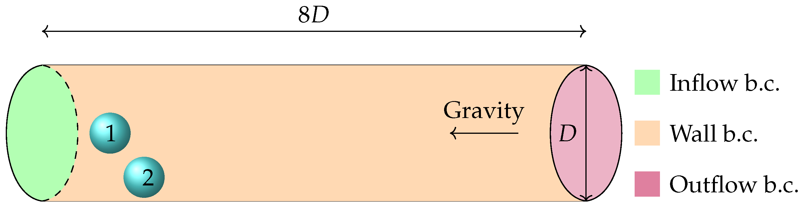
The simulation setup can be observed in Figure 2. A vertical circular channel is represented, with a non-dimensional diameter $d=1$ and length $l=8$. At one end, an inflow with a uniform non-dimensional velocity $v=1$ is set, and at the other end, an outflow where pressure $p=0$ is positioned. The walls along the channel have no slip boundary conditions. Two bubbles are positioned inside the channel. The bubble at the center, labeled the free bubble, has its center positioned at $p_1=(1,0,0)$, while the bubble at the side, labeled the shear bubble, has its center positioned at $p_2=(1.3,0,-0.31)$. Both bubbles are initially spherical in shape and have a diameter of $D_1=D_2=0.3$. For reference, the center of the channel’s bottom is positioned at $O=(0,0,0)$.

In relation to the initial positioning of the bubbles, our objective was to examine the influence of a bubble’s wake on nearby bubbles within a circular channel. The positions of the bubbles within the channel were deliberately selected so that they have different velocities, enabling one bubble to overtake the other. Additionally, the diameters were determined to ensure that, if the bubbles maintain a straight trajectory along the x-axis, they would closely approach each other at the moment of passing.

By inputting the fluid properties specified in the previous paragraph into the Morton number equation, three pairs of Reynolds and Weber numbers were selected to be simulated. The first one is $We=10$ and $Re=64$, the second one is $We=20$ and $Re=107$, and the third one is $We=40$ and $Re=180$. All three cases used $Fr=1$. Simulations with those parameters were executed with and without gravity forces, totaling six scenarios. All simulations were conducted over 300 time steps of $dt=0.01$, resulting in $t=3$ non-dimensional time units, equivalent in seconds to $t=3$ s.

Figure 3 presents the results of the simulation executed with Weber and Reynolds $We=10$ and $Re=64$ at $t=2$, $t=9$, $t=14$, and $t=19$. For the given parameters, there is very little difference between the results obtained with and without gravity forces. In the simulation executed with gravity, the bubbles travel further ahead in the channel, but the shape and position relative to one another are very similar, as can be seen in Figure 4. The bubble near the wall undergoes some deformation due to the shear forces caused by the velocity gradient. There is very little influence on the free-bubble trajectory due to the shear bubble. After the free bubble passes the shear bubble, it is carried by the flow normally.

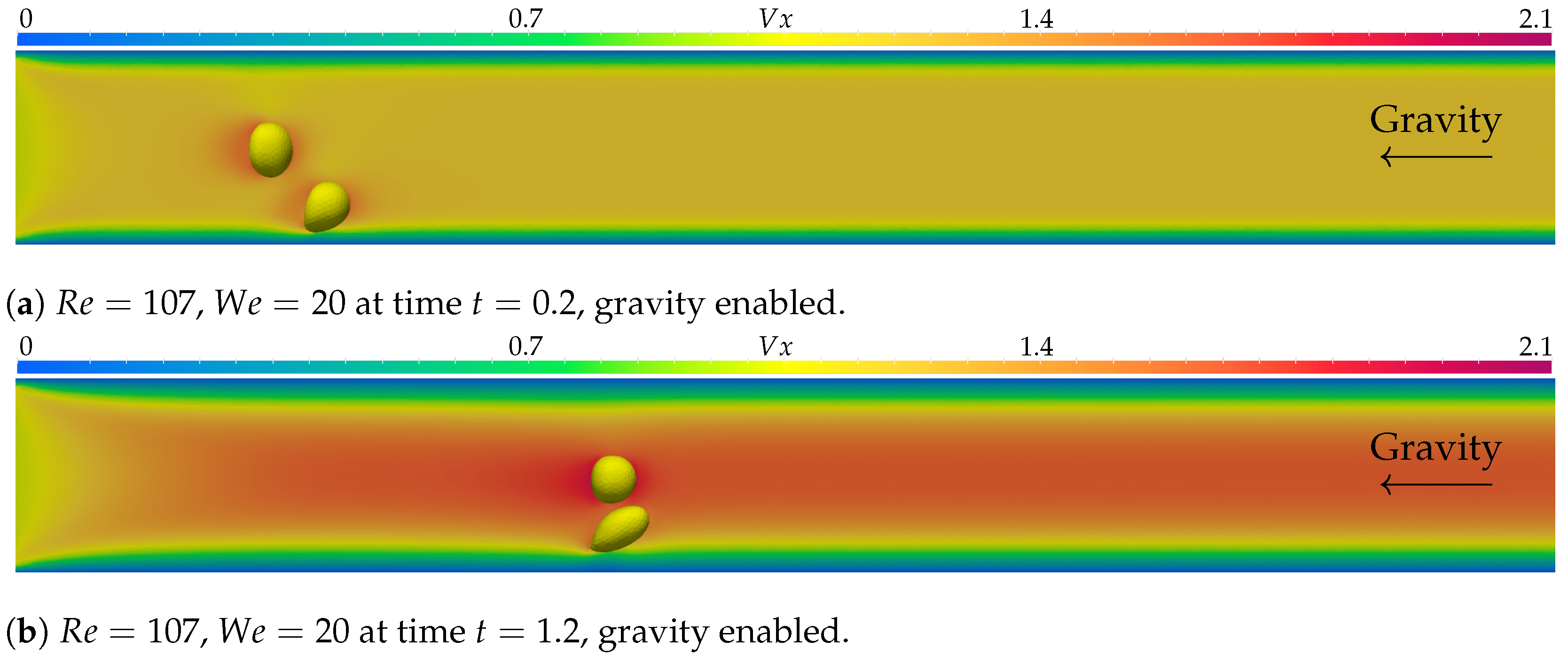
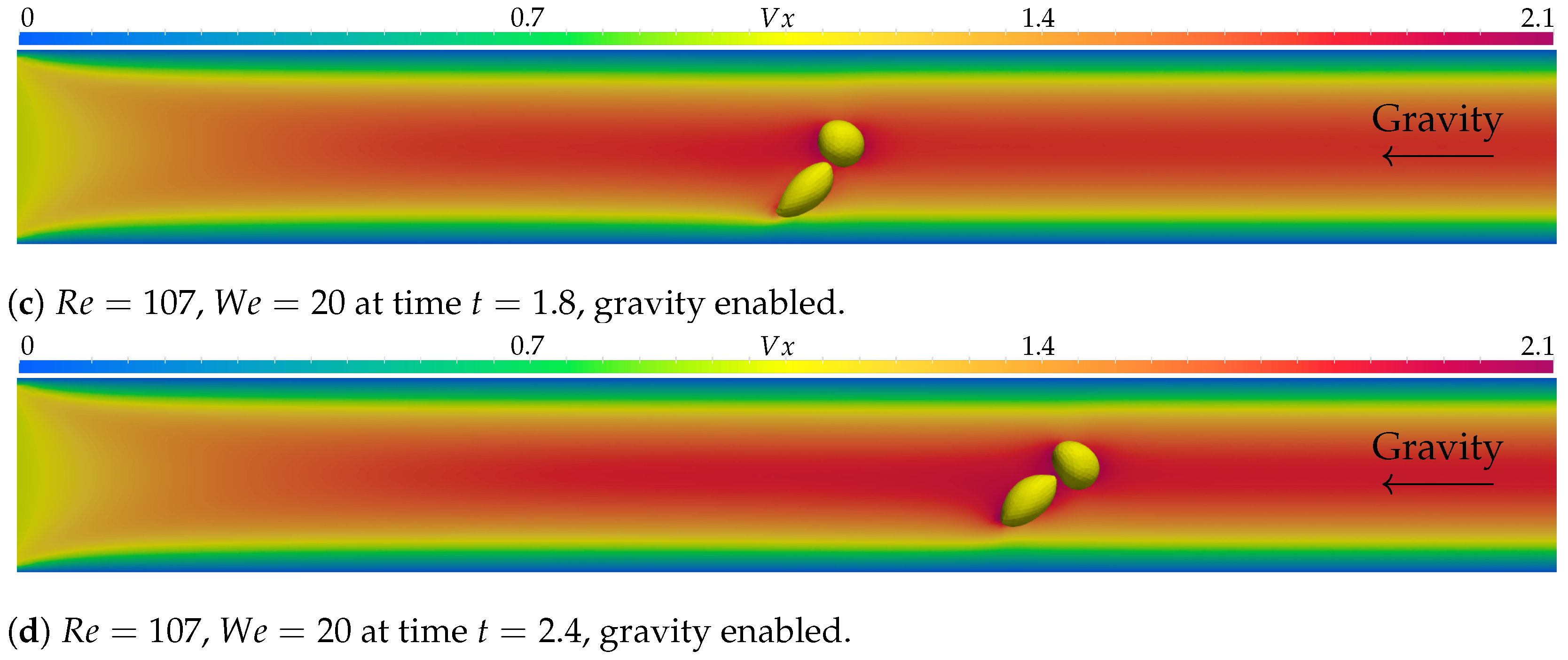
Figure 5 presents the results of the simulation executed with the Reynolds number $Re=107$ and the Weber number $We=20$, with no gravity forces, while Figure 6 shows the results with the same parameters but with gravity forces active. The times presented are $t=2$, $t=12$, $t=18$, and $t=240$. The results for the bubble simulation with no gravity forces are very similar to those of the previous simulations with $Re=64$ and $We=10$.

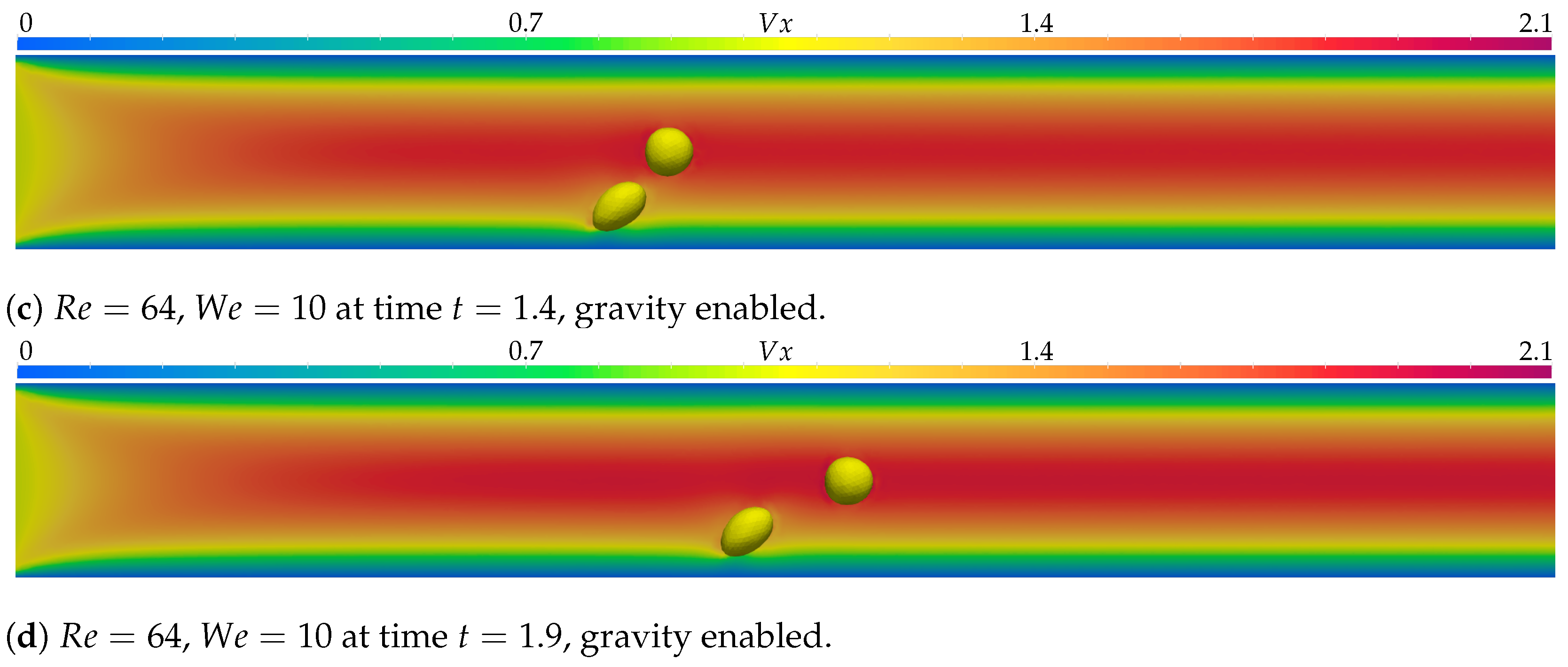
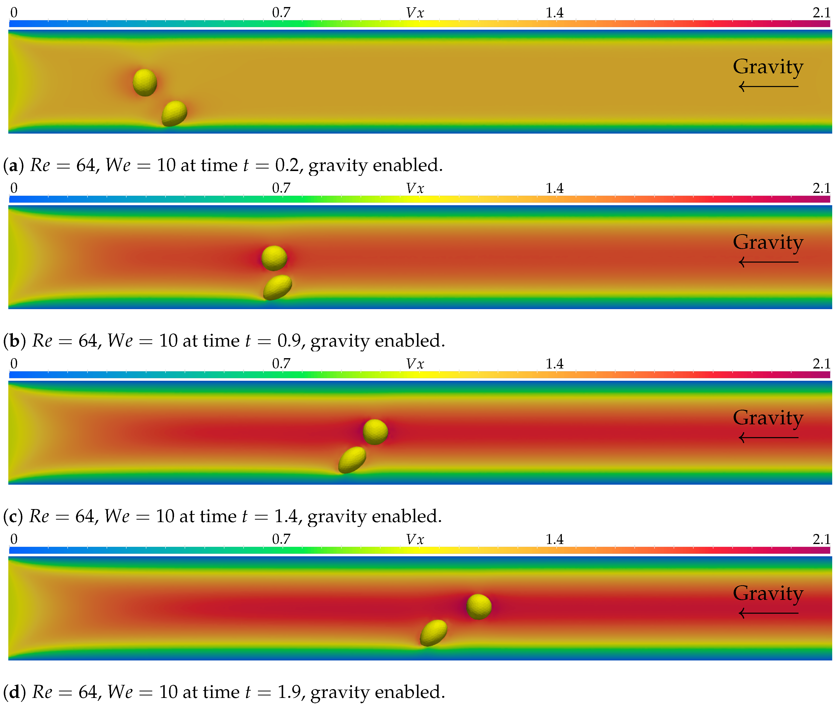
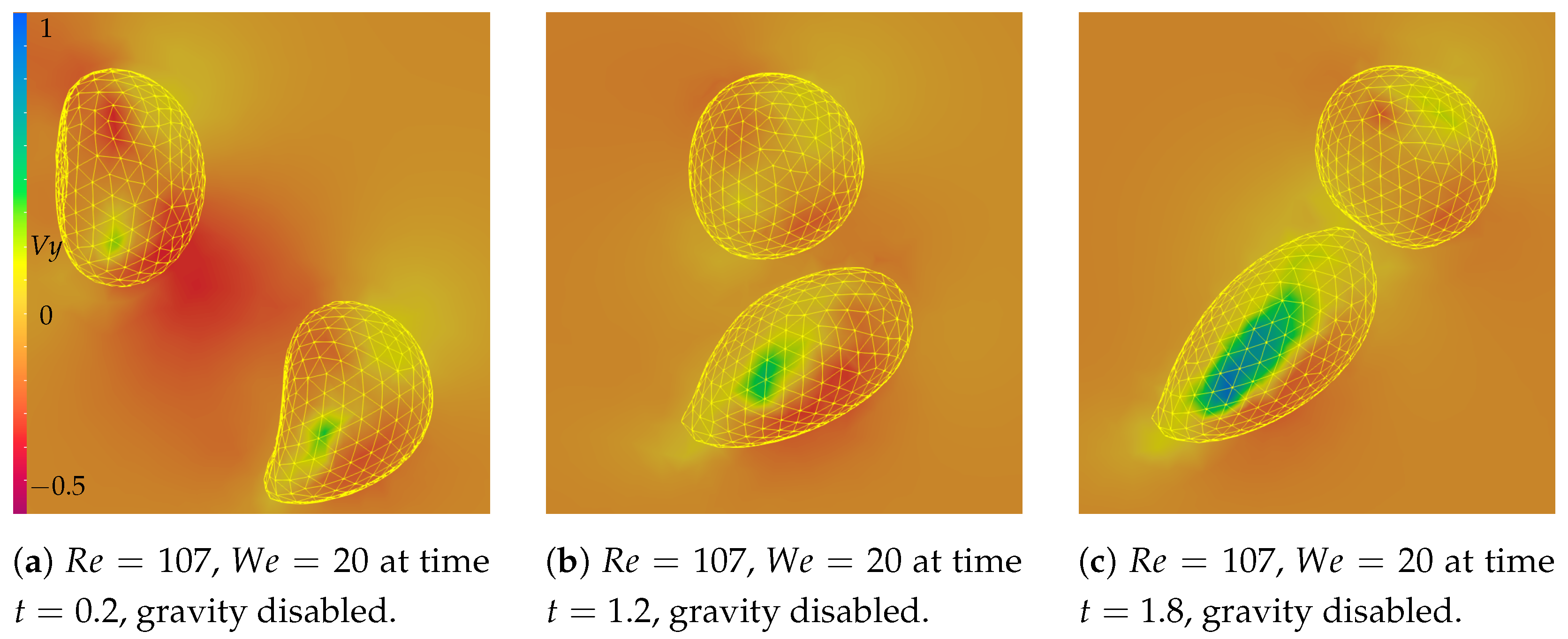
However, when gravity forces are active, there is some variation. The shear bubble suffers significantly more deformation and approaches the free bubble at the moment the free bubble passes it. The free bubble interacts with the shear bubble, changing shape as it moves along the flow, and the shear bubble appears to be trapped in the free bubble’s wake, increasing its velocity compared to the simulation with no gravity forces active and approaching the center of the channel. This effect can be observed in Figure 7, along with the velocity fields that originate it.

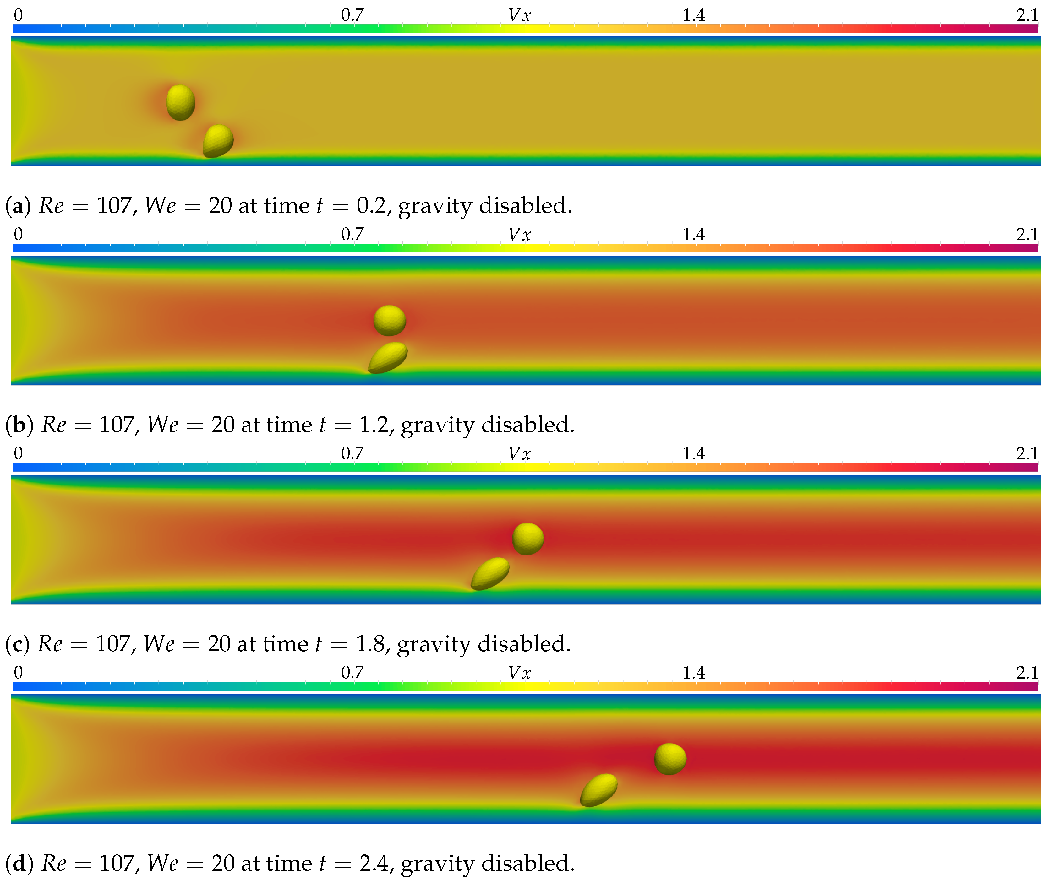
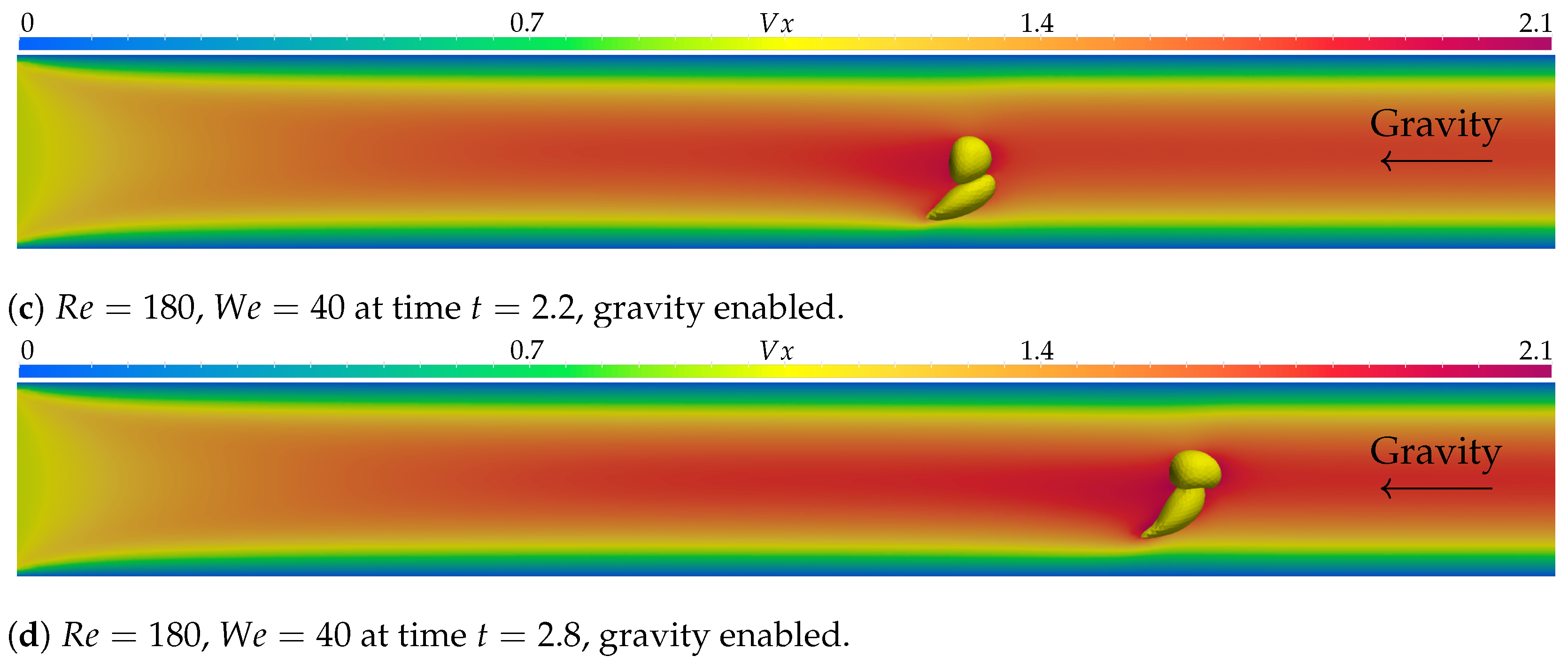
Figure 8 presents the results of the simulation executed with the Reynolds number $Re=180$ and the Weber number $We=40$, with no gravity forces, while Figure 9 shows the results with the same parameters but with gravity forces active. The times presented are $t=2$, $t=12$, $t=18$, and $t=240$. The simulation with no gravity presents similar results to those of other simulations without gravity, with slightly more deformation for both bubbles due to lower viscosity and lower surface tension forces. The simulation executed with gravity forces turned on offers some interesting results. The shear bubble undergoes the most deformation, being stretched toward the center, moving into the free bubble’s trajectory, and causing a contact. The current two-phase bubble-merging model was disabled for all simulations, since coalescence is not the aim of the present research, but it can be argued that it could occur under these conditions.

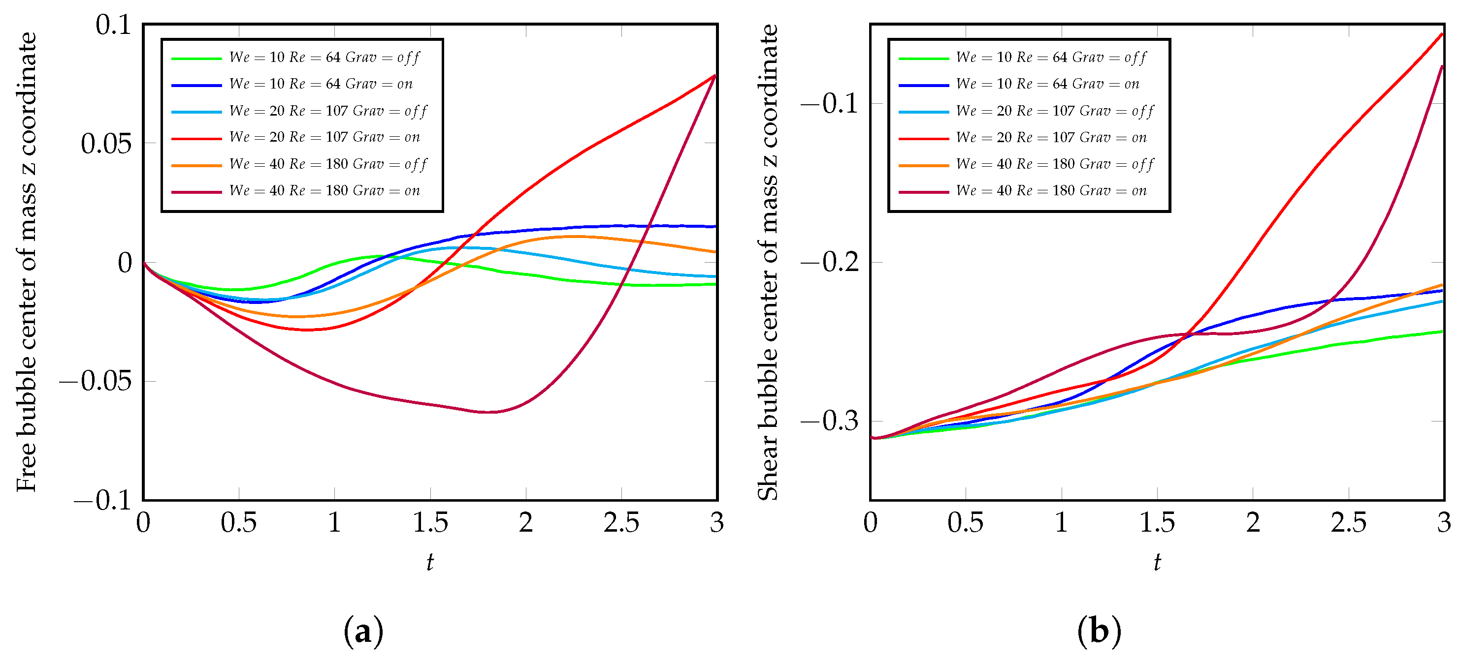
Figure 10 presents the change in the z-coordinate for both bubbles in all six simulations. In all simulations, some influence can be seen in the plot, but the impact in scenarios with $We=10$ and $We=20$ is not as significant. The remaining simulations, with $We=40$, show some relevant influence on both bubbles’ trajectories, especially the simulations with gravity forces.

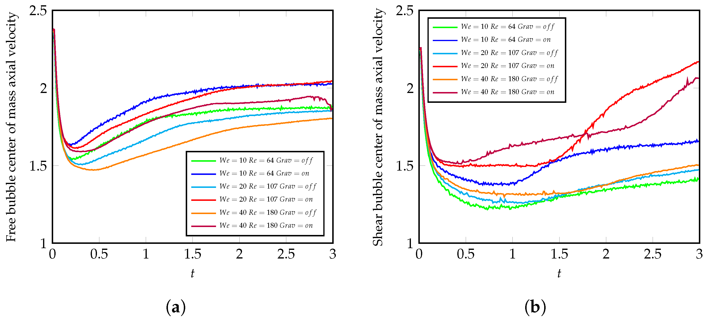
In Figure 11, the x-direction velocity component for both bubbles is presented. It can be inferred from the plot that the free bubble is slowed down by the shear bubble’s presence, up until the point where the free bubble overtakes it. It is also evidenced that the shear bubble accelerates after the free bubble’s passage, especially in the simulations where gravity effects are enabled.

4. Conclusions

In this study, we investigated the behavior of two bubbles transported by a fluid flow within a circular channel using numerical simulations to assess their dynamics. We employed a decoupled mesh method to accurately represent the interface between the two phases, akin to a front-tracking approach. Six different scenarios with varying flow parameters were simulated. The observed deformation of gas bubbles can be attributed to both their position inside the channel and the drag forces acting on the bubble. There is a velocity gradient in the channel radius direction, from the maximum velocity at the center of the channel to zero velocity at the walls. The bubbles are advected by the channel velocity fields, and this gradient provokes a shearing effect, which is most evident on the bubble near the wall due to the steeper velocity gradient in that region. The bubbles also suffer from the drag forces affecting them, especially at higher Weber numbers, where the surface tension, which works to keep the bubbles in a spherical shape, is not as strong. These deformations have the potential to culminate in bubble breakup. In cases of higher viscosity and surface tension, the mutual influence between bubbles is reduced, and their shape is preserved. Conversely, in less viscous flows, we observed an instance where one bubble entraps the other in its wake, increasing its velocity.

Our findings also indicate a trend where the shear bubbles migrate toward the center of the channel. The reason for this can be vertical velocities induced by the passing of the free bubble. As the free bubble approaches, it generates velocity away from its apex, which pushes the shear bubble. After passing, it drags the shear bubble upwards. This effect appears more significant in the example with $Re=107$, $We=20$, and gravity forces enabled.

These findings can guide engineers to make informed decisions when designing more efficient microchannel heat sinks and CO₂ injection solutions.