Shear Flows of Dilatant Fluids with Limited Shear Rates: Analytical Results and Linear Stability Analysis

Abstract

In this paper, we study the simple shear flows of a class of dilatant fluids with a limited shear rate. This class of fluids is characterized by shear thickening behavior in which the apparent viscosity tends to infinity as the modulus of the stress approaches a finite threshold. The apparent viscosity function is a logarithmic type with two material parameters. We considered this specific form because it fits very well with the flow curves of some granular suspensions for specific values of the material parameters. Despite the nonlinearity of the constitutive law, it is possible to determine explicit steady-state solutions for a simple shear flow, namely (i) the channel flow; (ii) the flow between coaxial cylinders, and (iii) the flow down an inclined plane. We performed a two-dimensional linear stability analysis to investigate the onset of possible instabilities of the steady basic flow, putting into evidence the dependency of the critical Reynolds number on the material parameters.

1. Introduction

Shear thickening (or dilatant) fluids are part of a special class of non-Newtonian fluids in which the viscosity increases with the shear rate. One of the first investigations on shear-thickening fluids is probably the one by Metzner and Whitlock [1] who studied a suspension of titanium dioxide (TiO${}_2$) particles in water. They showed that the relation between the shear stress and the shear rate is nonlinear with the apparent viscosity that grows with the increasing shear rate. For the elevated TiO${}_2$ volume fraction, the stress curve appears to almost diverge as the shear rate increases. The most dramatic scenario of this type of behavior is that of discontinuous shear thickening (DST), where viscosity becomes infinite for a finite value of the shear rate and the material goes from fluid-like to solid-like, see [2,3,4].

In the recent past, many works have investigated the nature of shear-thickening and DST fluids, see [5,6,7,8]. In particular, the crucial effects of frictional contact forces (in the framework of jamming transition) on the shear-thickening behaviors of the fluid have been observed. As observed in [9], the scale of the stress (where the stress–shear rate constitutive law starts to show large growth) can be attributed to the interfacial tension forces, which increase abruptly due to the dramatic constraint of jamming.

In general, dense mixtures of granules and liquids behave as dilatant fluids, a classical example being cornstarch and water. Some fluids, such as high-concentration suspensions, insoluble polymer systems, clay, and quicksand display shear-thickening behaviors [10]. Although a large majority of fluids exhibit pseudo-plastic (or shear-thinning) behaviors [11], shear-thickening fluids are also ubiquitous in a variety of practical applications, from damping devices to machine mounts, as well as in the manufacturing of body armor [12], where the shear-thickening properties are exploited to dampen the impacts of a bullet.

Regarding the counterintuitive behaviors of dilatant fluids, one can search the web for a video of one running on a pool filled with cornstarch and water as if it was an actual rigid surface, but sinking into it when walking or standing still. At the microscopic level, experiments have shown that dense suspensions are basically frictionless for low confining pressure, while the transition from low to high friction occurs with normal stress near the critical stress, see [13].

The constitutive law of a shear-thickening fluid is commonly represented by a function in which the shear stress is expressed as a function of the shear rate and in which the first derivative of that function increases with the shear rate. The most common example is that of power law dilatant fluids, where the apparent viscosity is a given positive power of the shear rate modulus. In the latter model, any arbitrarily large value of the shear rate can be attained if a sufficiently large shear stress is applied (the strain is not limited). This type of model is not appropriate when one considers a dilatant fluid in which the flow behavior is similar to that of a discontinuous shear-thickening fluid. In this case, we may consider a constitutive law in which there is a critical value to which the shear rate tends when the stress becomes infinite (limited strain model), see [4,14].

A very basic limited strain model is the one considered in [4] for a system formed by a mass, a dashpot, and an inextensible string; see Figure 1a. If the string is not completely extended, the response of the system is that of a Newtonian fluid, but when the string becomes fully extended, the response is that of a rigid body (the applied force produces no deformation). The constitutive relation is, thus, the one shown in Figure 1b, which can be seen as the “dual” of the Bingham constitutive law (the fluid flow only if the applied stress is below a certain threshold). The one-dimensional unsteady channel flow of a fluid with the constitutive law, as shown in Figure 1b, was studied in [4].

Figure 1. String-dashpot system (a) and constitutive law (b).

Let us suppose that the fluid is incompressible so that the Cauchy stress tensor can be written (in the paper, the starred quantities are always dimensional) as ${\mathbf{T}}^{\ast }=-p^{\ast }\mathbf{I}+{\mathbf{S}}^{\ast }$, where $p^{\ast }$ is the Lagrange multiplier due to the incompressibility constraint and ${\mathbf{S}}^{\ast }$ is the deviatoric part of the stress. The constitutive equation for a Newtonian fluid with a limited shear rate can be seen in [4,14].

$$\left\{\begin{array}{cc}{\mathbf{S}}^{\ast }=2{\mu }^{\ast }{\mathbf{D}}^{\ast },\hfill & \hfill \mid {\mathbf{S}}^{\ast }\mid ⩽{\tau }_c^{\ast },\\ \\ \mid {\mathbf{D}}^{\ast }\mid =d_c^{\ast },\hfill & \hfill \mid {\mathbf{S}}^{\ast }\mid ⩾{\tau }_c^{\ast },\end{array}\right.$$

(1)

where ${\mu }^{\ast }$ is the viscosity ($\left[{\mu }^{\ast }\right]=$ Pa·s), ${\tau }_c^{\ast }$ is the critical shear stress ($\left[{\tau }_c^{\ast }\right]=$ Pa), and $d_c^{\ast }$ is the critical shear rate ($\left[d_c^{\ast }\right]=$ s${}^{-1}$). The quantities

$$\mid {\mathbf{S}}^{\ast }\mid ={\left[{\displaystyle \frac{1}{2}}{\mathbf{S}}^{\ast }·{\mathbf{S}}^{\ast }\right]}^{1/2},\mid {\mathbf{D}}^{\ast }\mid ={\left[{\displaystyle \frac{1}{2}}{\mathbf{D}}^{\ast }·{\mathbf{D}}^{\ast }\right]}^{1/2},$$

represent the norm of the deviatoric part of the stress ${\mathbf{S}}^{\ast }$ and the symmetric part of the velocity gradient ${\mathbf{D}}^{\ast }$, respectively. Looking at Figure 1b, it is evident that if we plot $\mid {\mathbf{S}}^{\ast }\mid$ vs. $\mid {\mathbf{D}}^{\ast }\mid$, we obtain a graph (the stress is not determinate for $\mid {\mathbf{D}}^{\ast }\mid =d_c^{\ast }$); hence, it is more natural to express $\mid {\mathbf{D}}^{\ast }\mid$ vs. $\mid {\mathbf{S}}^{\ast }\mid$, so that the relation is an actual function (see [15] for a discussion on the material defined by implicit constitutive equations).

Relation (1) has a singularity in the first derivative at $(d_c^{\ast },{\tau }_c^{\ast })$, which can be smoothed if one takes, for instance,

$${\mathbf{S}}^{\ast }=2{\mu }_{\mathrm{eff}}^{\ast }(\mid {\mathbf{D}}^{\ast }\mid ){\mathbf{D}}^{\ast },$$

(2)

where the effective viscosity is given by

$${\mu }_{\mathrm{eff}}^{\ast }\left({\xi }^{\ast }\right)={\displaystyle \frac{1}{2{\xi }^{\ast }{a}^{\ast }}}ln\left({\displaystyle \frac{b^{\ast }}{b^{\ast }-2{\xi }^{\ast }}}\right).$$

(3)

The constitutive relation (2), (3) was selected because it fits the experimental flow curves of dense suspensions, see [1,16].

In Figure 2, we plotted the relation (2), taking the norms on both sides. We normalized $\mid {\mathbf{S}}^{\ast }\mid$ with $1/\left(2a^{\ast }\right)$ and $\mid {\mathbf{D}}^{\ast }\mid$ with $b^{\ast }/2$. The parameter $a^{\ast }$ has the dimension of the inverse of the pressure, while the dimension of $b^{\ast }$ is that of a shear rate. In Figure 3, we plot the effective viscosities (3) for some values of $a^{\ast }$ and with $b^{\ast }=18{\mathrm{s}}^{-1}$. The ranges for these values are consistent with the experimental data of [16]. We notice that for sufficiently large values of $a^{\ast }$, the constitutive behavior of the fluid is similar to that of an inviscid fluid (the effective viscosity is nearly zero almost everywhere in the range $(0,b^{\ast })$) except for a small boundary layer near the critical value $b^{\ast }$, where the viscosity becomes arbitrarily large (rigid body behavior). The behaviors of the fluids for small values of $\mid {\mathbf{D}}^{\ast }\mid$ are similar to those of Newtonian fluids with constant viscosity

$$\underset{{\xi }^{\ast }\to 0}{lim}{\mu }_{\mathrm{eff}}^{\ast }\left({\xi }^{\ast }\right)={\displaystyle \frac{1}{a^{\ast }{b}^{\ast }}}.$$

Hence, parameters $a^{\ast }$ and $b^{\ast }$ determine the “almost constant” viscosity of the fluid for small shear rates, whereas $b^{\ast }/2$ is the limiting value for the shear rate.

Figure 2. Constitutive law (2) in which the shear rate is normalized with $b^{\ast }/2$ and the shear stress with $1/2a^{\ast }$.

The behaviors of parameters $a^{\ast }$ and $b^{\ast }$ with the particle concentration $\varphi$ are related to the shear-thickening effects due to the particle concentrations. From [1,16], it is evident that the parameter $b^{\ast }$ is a decreasing function of $\varphi$. This is physically consistent since the limiting shear rate increases if the particle’s volume fraction decreases because the frictional effects between particles become less pronounced. The same is true for $a^{\ast }$ as the apparent viscosity (which is proportional to $1/a^{\ast }$) must decrease as the volume fraction decreases. The exact dependencies of the parameters $a^{\ast }$ and $b^{\ast }$ on $\varphi$ will surely involve some material constants that take into account the particular suspension considered. The definition of such a dependency is beyond the scope of this paper and certainly would require more experimental data.

The constitutive law (3) does not take into account the possibility that the slope of the constitutive curve may start to decrease after a certain value of the shear stress. In practice, it does not allow one to consider the S-shaped behavior exhibited by the suspension. Here, we are only interested in the range of stresses for which the slope of the shear stress shear rate curve is monotonically increasing and tends to be infinite, such as the ones of [1,16].

Figure 3. Plot of the effective viscosity ${\mu }_{\mathrm{eff}}^{\ast }$ given in (3) as a function of the shear rate $2{\xi }^{\ast }$ for different values of $a^{\ast }$ and $b^{\ast }=18{\mathrm{s}}^{-1}$. The values of these parameters are taken from [16].

In this work, we consider the responses of types (2) and (3) since we have seen that they describe quite well the experimental flow curves of some dense suspensions. In particular, we consider Figure 4 and Figure 5, in which $a^{\ast }$ and $b^{\ast }$ are selected to fit the experimental curves of two types of suspensions, namely a $47\%$ TiO${}_2$ suspension in Figure 4 and a $50\%$ cornstarch suspension in Figure 5. The experimental data in Figure 4 and Figure 5 are taken from [1,16] respectively. This paper is devoted to the study of some simple shear flow of fluid with a constitutive law of types (2) and (3). In particular, we focus on three types of flow, i.e., (i) planar channel flow; (ii) the flow between coaxial cylinders; and (iii) the flow down an inclined plane. Despite the nonlinearity of (3), we shall see that in all geometrical settings considered in this paper, it is always possible to determine an analytical steady-state solution. For each problem, the flow equations are scaled appropriately so that the velocity field can be expressed in terms of the Reynolds number and other non-dimensional material (i.e., not depending on the flow) parameters. Because of the boundedness of the shear rate, in some geometrical settings, the Reynolds number happens to be bounded, meaning that the range of velocities that can be attained by increasing the force that drives the motion is limited. This is consistent with the shear thickening and limited strain nature of the fluid, where friction forces between layers (viscosity) grow with the shear stress, preventing the velocity from increasing unboundedly. Models of types (2) and (3) are useful because one can explicitly determine the velocity and stress profiles in the simple flow, but also because they allow approximating the DST models by avoiding the intrinsic singularities in the constitutive equations.

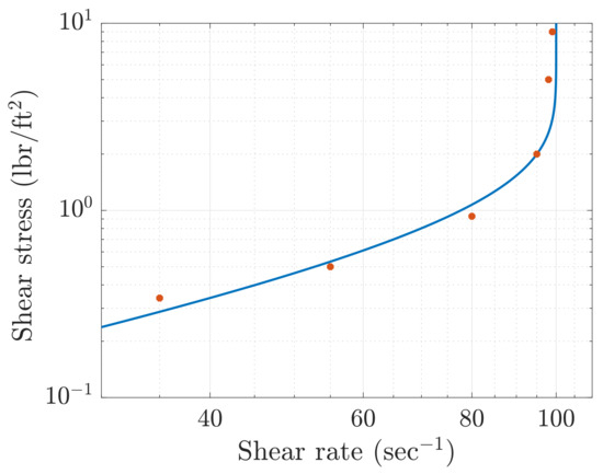
Figure 4. Flow curve (shear stress vs. shear rate) for TiO${}_2$ suspension (47%), see Figure 2 in [1]. Experimental data (stars) and fitting curve (continuous). Fitting parameters $a^{\ast }=1.5$ (ft${}^2$/lbr), $b^{\ast }={10}^2$ s${}^{-1}$.

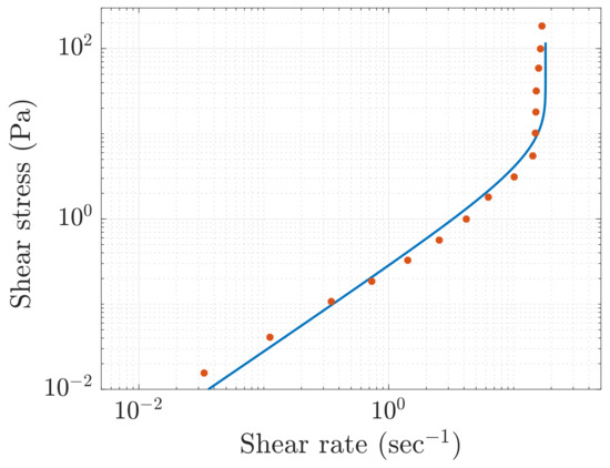
Figure 5. Flow curve (shear stress vs. shear rate) for the cornstarch suspension (50%), see Figure 1 in [16]. Experimental data (stars) and fitting curve (continuous). Fitting parameters $a^{\ast }=0.2$ (Pa${}^{-1}$), $b^{\ast }=18$ s${}^{-1}$.

In addition to determining the steady-state solutions of the basic flow, we performed a modal stability analysis to investigate the onset of possible instabilities. In the flow considered here, the critical Reynolds number is an increasing function of both $a^{\ast }$ and $b^{\ast }$. Looking at Figure 3, we may explain this behavior by observing that the increase of $a^{\ast }$ (this is also true for the increase of $b^{\ast }$) results in the formation of boundary layers with high viscosity near the rigid walls that tend to stabilize the flow. This type of behavior has also been put into evidence in a recent paper [17] for the stress power-law fluids.

The paper is organized as follows. In Section 2, we derive the mathematical formulation of the problem and focus on (i) planar channel flow; (ii) the flow between coaxial cylinders; and (iii) the flow down an inclined plane. In Section 3, we perform the linear stability analysis for the above-mentioned simple flow. The last section is devoted to conclusions and perspectives.

2. The Mathematical Model

Let us consider the following constitutive equation

$${\mathbf{T}}^{\ast }=-p^{\ast }\mathbf{I}+{\mathbf{S}}^{\ast },{\mathbf{S}}^{\ast }=2{\mu }_{\mathrm{eff}}^{\ast }(\mid {\mathbf{D}}^{\ast }\mid ){\mathbf{D}}^{\ast },$$

(4)

$${\mu }_{\mathrm{eff}}^{\ast }(\mid {\mathbf{D}}^{\ast }\mid )={\displaystyle \frac{1}{2\mid {\mathbf{D}}^{\ast }\mid a^{\ast }}}ln\left({\displaystyle \frac{b^{\ast }}{b^{\ast }-2\mid {\mathbf{D}}^{\ast }\mid }}\right),$$

(5)

and let us rescale the dimensional variables with

$${\mathbf{x}}^{\ast }=L^{\ast }\mathbf{x},t^{\ast }=\left(L^{\ast }{U}^{{\ast }^{-1}}\right)t,$$

(6)

$$p^{\ast }={\mathsf{\Pi }}^{\ast }p,{\mathbf{S}}^{\ast }=a^{\ast -1}\mathbf{S},{\mathbf{D}}^{\ast }=\left(U^{\ast }{L}^{{\ast }^{-1}}\right)\mathbf{D}.$$

(7)

Introducing the quantities $b=L^{\ast }{b}^{\ast }{U}^{{\ast }^{-1}}$ and $\mathsf{\Pi }={\mathsf{\Pi }}^{\ast }{a}^{\ast }$, we write the non-dimensional mass and momentum balance (neglecting body forces) as

$$\left\{\begin{array}{c}\mathrm{div}\mathbf{v}=0,\hfill \\ \\ \mathsf{Re}\dot{\mathbf{v}}=-\mathsf{\Pi }\nabla p+\mathrm{div}\left(\mathbf{S}\right),\hfill \end{array}\right.$$

(8)

where $\mathsf{Re}={\rho }^{\ast }{U}^{{\ast }^2}{a}^{\ast }$ is the Reynolds number. The non-dimensional constitutive equation becomes:

$$\mathbf{S}=\underset{={\mu }_{\mathrm{eff}}}{\underbrace{\left[{\displaystyle \frac{1}{2\mid \mathbf{D}\mid }}ln\left({\displaystyle \frac{b}{b-2\mid \mathbf{D}\mid }}\right)\right]}}2\mathbf{D}.$$

(9)

We notice that b and $\mathsf{Re}$ are related by

$$b={\displaystyle \frac{\mathsf{\Gamma }}{\sqrt{\mathrm{Re}}}},\mathsf{\Gamma }=L^{\ast }{b}^{\ast }\sqrt{{\rho }^{\ast }{a}^{\ast }}$$

(10)

where $\mathsf{\Gamma }$ is a non-dimensional material parameter (it does not depend on the flow). From [1,16], we know that typically $\mathsf{\Gamma }=O\left(10\right)$.

2.1. Channel Flow Driven by a Pressure Gradient

Let us consider problems (8) and (9) for a fluid flowing in a planar channel of length $L^{\ast }$ and constant width $2H^{\ast }$ driven by a pressure gradient $\Delta p^{\ast }=p_{\mathrm{in}}^{\ast }-p_{\mathrm{out}}^{\ast }>0$. For simplicity, here we assume that $H^{\ast }=L^{\ast }$, but minor changes allow one to consider the cases in which they are different. In this situation, it is natural to select ${\mathsf{\Pi }}^{\ast }=\Delta p^{\ast }$ and $\mathsf{\Pi }=\Delta p^{\ast }{a}^{\ast }$. We look for a stationary solution of problem (8) in the form $\mathbf{v}=u\left(y\right)\mathbf{i}$, $p=p(x,y)$, so that the incompressibility constraint $\mathrm{div}\mathbf{v}=0$ is automatically satisfied. The problem becomes

$$\left\{\begin{array}{c}0=-\mathsf{\Pi }{\displaystyle \frac{\partial p}{\partial x}}+{\displaystyle \frac{\partial S_{12}}{\partial y}},\hfill \\ \\ {\displaystyle \frac{\partial p}{\partial y}}=0.\hfill \end{array}\right.$$

(11)

We immediately realize that

$${\displaystyle \frac{\partial p}{\partial x}}=-1,\mid \mathbf{D}\mid ={\displaystyle \frac{\mid u_y\mid }{2}},S_{12}=\mathrm{sign}\left(u_y\right)ln\left({\displaystyle \frac{b}{b-\mid u_y\mid }}\right).$$

(12)

Integrating (11)${}_1$ and exploiting (12), we find

$${\displaystyle \frac{\partial u}{\partial y}}=-\mathrm{sign}\left(u_y\right)b\left[1-exp\left(-\mathsf{\Pi }\mid y\mid \right)\right].$$

(13)

Integrating once more with the no-slip boundary conditions $u(\pm 1)=0$, we have

$$u\left(y\right)=b\left[1-\mid y\mid -{\displaystyle \frac{1}{\mathsf{\Pi }}}\left(exp(-\mathsf{\Pi }\mid y\mid )-exp(-\mathsf{\Pi })\right)\right],$$

(14)

which provides the velocity profile in the whole domain. We may select the characteristic velocity $U^{\ast }$ so that the velocity of the fluid in the centerline is 1. Imposing $u\left(0\right)=1$, we find

$$b={\displaystyle \frac{\mathsf{\Pi }}{\mathsf{\Pi }-1+e^{-\mathsf{\Pi }}}}⟺\mathsf{\Pi }={\displaystyle \frac{b}{b-1}}+\mathcal{W}\left[{\displaystyle \frac{b}{1-b}}exp\left({\displaystyle \frac{b}{1-b}}\right)\right],$$

(15)

where $\mathcal{W}\left(z\right)$ is the zero branch of the Lambert function, see [18]. Relation (15)${}_1$ is equivalent to setting

$$U^{\ast }=L^{\ast }{b}^{\ast }\left[{\displaystyle \frac{\Delta p^{\ast }{a}^{\ast }-1+exp(-\Delta p^{\ast }{a}^{\ast })}{\Delta p^{\ast }{a}^{\ast }}}\right].$$

(16)

As one can easily realize, the increase of the pressure drop $\Delta p^{\ast }$ is equivalent to the increase in the characteristic velocity $U^{\ast }$, but since the shear rate is limited, the velocity $U^{\ast }$ is bounded from above (it cannot become arbitrarily large). Indeed, for $\Delta p^{\ast }\in (0,\infty )$, we have $U^{\ast }\in (0,L^{\ast }{b}^{\ast })$, so that $b>1$, no matter how strong the applied pressure drop $\Delta p^{\ast }$ is. We notice that

$$U^{\ast }=\sqrt{{\displaystyle \frac{\mathsf{Re}}{{\rho }^{\ast }{a}^{\ast }}}},\Rightarrow b={\displaystyle \frac{L^{\ast }{b}^{\ast }\sqrt{{\rho }^{\ast }{a}^{\ast }}}{\sqrt{\mathsf{Re}}}}={\displaystyle \frac{\mathsf{\Gamma }}{\sqrt{\mathsf{Re}}}}>1.$$

(17)

From the inequality in (17), we realize that the Reynolds number is bounded for this type of flow since from relation (16), the velocity $U^{\ast }\in (0,L^{\ast }{b}^{\ast })$. In particular, $\mathsf{Re}\in (0,{\mathsf{\Gamma }}^2)$ and $b=b\left(\mathsf{Re}\right)$ are functions of the Reynolds number. Inserting (15)${}_1$ into (14), and rearranging, we finally find the velocity field expressed in terms of the Reynolds number

$$\left\{\begin{array}{c}u\left(y\right)=\left[1-{\displaystyle \frac{\mathsf{\Pi }\mid y\mid -1+e^{-\mathsf{\Pi }\mid y\mid }}{\mathsf{\Pi }-1+e^{-\mathsf{\Pi }}}}\right],\hfill \\ \\ \mathsf{\Pi }={\displaystyle \frac{b}{b-1}}+\mathcal{W}\left[{\displaystyle \frac{b}{1-b}}exp\left({\displaystyle \frac{b}{1-b}}\right)\right],b={\displaystyle \frac{\mathsf{\Gamma }}{\sqrt{\mathsf{Re}}}},\mathsf{Re}\in (0,{\mathsf{\Gamma }}^2).\hfill \end{array}\right.$$

(18)

In Figure 6, we show the velocity profile (18) for $\mathsf{Re}<{\mathsf{\Gamma }}^2$, with $\mathsf{\Gamma }=15$. We observe that the velocity profile assumes a wedge-like shape as $\mathsf{Re}$ approaches the limit value ${\mathsf{\Gamma }}^2$.

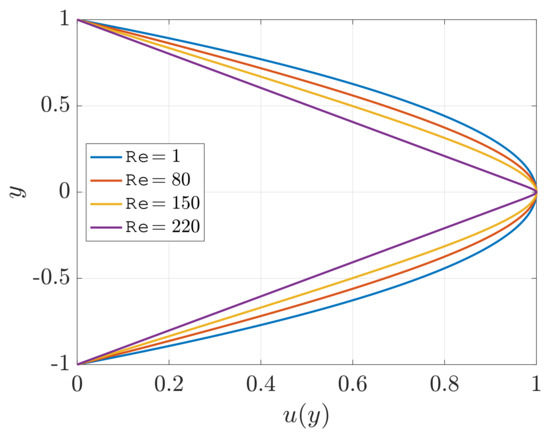
Figure 6. Velocity profiles (18) for various $\mathsf{Re}<{\mathsf{\Gamma }}^2$, $\mathsf{\Gamma }=15$.

We observe that

$$\mathsf{Re}=\underset{={\mathsf{\Gamma }}^2}{\underbrace{{\rho }^{\ast }{a}^{\ast }{L}^{{\ast }^2}{b}^{{\ast }^2}}}\underset{<1}{\underbrace{\left[{\displaystyle \frac{\Delta p^{\ast }{a}^{\ast }-1+exp(-\Delta p^{\ast }{a}^{\ast })}{\Delta p^{\ast }{a}^{\ast }}}\right]}}<{\mathsf{\Gamma }}^2$$

Hence, $\mathsf{Re}$ is a monotonically increasing function of $a^{\ast }$. This is physically consistent since an increase in the value of $a^{\ast }$ means a decrease in the apparent viscosity, i.e., less resistance to the flow and, hence, a larger value of $\mathsf{Re}$, which is always bounded by ${\mathsf{\Gamma }}^2$. Notice that ${\mathsf{\Gamma }}^2$ is a function of $a^{\ast }$. Hence, if $a^{\ast }$ increases, ${\mathsf{\Gamma }}^2$ also increases. For the other types of flow that will be studied in the next sections, we can make analogous considerations.

2.2. Flow between Coaxial Cylinder

In this section, we consider the flow between coaxial cylinders with inner and outer radii $R_1^{\ast }$ and $R_2^{\ast }$, respectively. Without loss of generality, we may assume that the inner cylinder is fixed whereas the outer cylinder rotates anticlockwise with angular velocity ${\mathsf{\Omega }}_2^{\ast }$. Distance is scaled with $R_2^{\ast }$, velocity is rescaled with ${\mathsf{\Omega }}_2^{\ast }{R}_2^{\ast }$, and pressure is rescaled with $a^{{\ast }^{-1}}$. Exploiting cylindrical coordinates, we look for a steady solution of the type:

$$\mathbf{v}=u\left(r\right){\mathbf{e}}_{\theta },p=p\left(r\right).$$

(19)

The only non-zero component of the deviatoric stress tensor is $S_{r\theta }$. Introducing the angular velocity $\omega \left(r\right)=u\left(r\right)/r$, it is easy to see that

$$\mid \mathbf{D}\mid ={\displaystyle \frac{1}{2}}\mid r{\omega }^{\prime }\mid ={\displaystyle \frac{r}{2}}{\omega }^{\prime },$$

(20)

where ${}^{\prime }=d/dr$ and where ${\omega }^{\prime }⩾0$, since the non-dimensional angular velocity w must be an increasing function of r ranging between 0 (inner cylinder) and 1 (outer cylinder). Therefore,

$$S_{r\theta }=ln\left({\displaystyle \frac{b}{b-r{\omega }^{\prime }}}\right).$$

(21)

The mass balance is automatically satisfied, while the momentum balance is reduced to

$$\left\{\begin{array}{c}-\mathsf{Re}{\displaystyle \frac{u^2}{r}}=-{\displaystyle \frac{\partial p}{\partial r}}\hfill \\ \\ 0={\left[r^2{S}_{r\theta }\right]}^{\prime }={\left[r^{2}ln\left({\displaystyle \frac{b}{b-r{\omega }^{\prime }}}\right)\right]}^{\prime }.\hfill \end{array}\right.$$

(22)

Integrating the second of (22), we find

$${\omega }^{\prime }\left(r\right)=b\left[{\displaystyle \frac{1-e^{-c/r^2}}{r}}\right],$$

(23)

with c being a positive constant to be determined. Integrating between $R_1=R_1^{\ast }/R_2^{\ast }<1$ and 1, we find (recall $\omega \left(R_1\right)=0$ and $\omega \left(1\right)=1$)

$${\int }_{R_1}^1{\omega }^{\prime }\left(r\right)dr=1=b\left[-ln{R}_1-{\displaystyle \frac{1}{2}}\left({\mathsf{E}}_1\left(c\right)-{\mathsf{E}}_1(c/R_1^2)\right)\right],$$

(24)

where

$${\mathsf{E}}_1\left(\xi \right)={\int }_{\xi }^{\infty }{\displaystyle \frac{e^{-z}}{z}}dz,$$

is the exponential integral. Equation (24) allows one to determine the constant c. Indeed let us rewrite (24) as

$$\gamma (c;R_1)=-ln{R}_1-{\displaystyle \frac{1}{2}}{\int }_c^{c/R_1^2}{\displaystyle \frac{e^{-z}}{z}}dz={\displaystyle \frac{1}{b}}.$$

(25)

The integrand function can be rewritten as

$${\displaystyle \frac{e^{-z}}{z}}={\displaystyle \frac{1}{z}}+\sum _{n=1}^{\infty }{\displaystyle \frac{{(-1)}^n{z}^{n-1}}{n!}},$$

(26)

so that

$$-{\displaystyle \frac{1}{2}}{\int }_c^{c/R_1^2}{\displaystyle \frac{e^{-z}}{z}}dz\approx ln\left(R_1\right)-\sum _{n=1}^{\infty }{\displaystyle \frac{{(-1)}^n}{2n!n}}\left[c^n-{\left({\displaystyle \frac{c}{R_1^2}}\right)}^n\right].$$

(27)

Hence, ${lim}_{c\to 0}\gamma (c;R_1)=0$ and since

$${\displaystyle \frac{1}{c}}⩾{\displaystyle \frac{1}{z}}⩾{\displaystyle \frac{R_1^2}{c}},$$

we obtain

$${\int }_c^{c/R_1^2}{\displaystyle \frac{e^{-z}}{z}}dz⩽{\displaystyle \frac{1}{c}}\underset{>0}{\underbrace{\left[e^{-c}-e^{-c/R_1^2}\right]}}\to 0,\mathrm{if}c\to \infty .$$

(28)

Therefore, ${lim}_{c\to \infty }\gamma (c;R_1)=-ln{R}_1>0$. Finally, we observe that $\partial \gamma /\partial c>0$, so that $\gamma$ is a positive strictly increasing function of c bounded between 0 and $-ln{R}_1>0$. The existence of a solution to (24) (or equivalently (25)) is, thus, guaranteed if $b^{-1}\in (0,-ln{R}_1)$, i.e., if

$${\mathsf{\Omega }}_2^{\ast }<b^{\ast }ln\left({\displaystyle \frac{R_2^{\ast }}{R_1^{\ast }}}\right).$$

(29)

Recalling that $\mathsf{Re}={\rho }^{\ast }{\left({\mathsf{\Omega }}_2^{\ast }{R}_2^{\ast }\right)}^2{a}^{\ast }$, we see that the existence of the solution is guaranteed if

$$\sqrt{\mathsf{Re}}<b^{\ast }{R}_2^{\ast }\sqrt{{\rho }^{\ast }{a}^{\ast }}ln\left({\displaystyle \frac{R_2^{\ast }}{R_1^{\ast }}}\right)=\mathsf{\Gamma }ln\left({\displaystyle \frac{R_2^{\ast }}{R_1^{\ast }}}\right)=-\mathsf{\Gamma }ln\left(R_1\right).$$

(30)

In conclusion, the Reynolds number is limited for this type of flow. Once c is determined, the solution to the problem becomes

$$\omega \left(r\right)={\displaystyle \frac{\mathsf{\Gamma }}{\sqrt{\mathsf{Re}}}}\left[ln\left({\displaystyle \frac{r}{R_1}}\right)-{\displaystyle \frac{1}{2}}\left({\mathsf{E}}_1\left({\displaystyle \frac{c}{r^2}}\right)-{\mathsf{E}}_1\left({\displaystyle \frac{c}{R_1^2}}\right)\right)\right],$$

(31)

where c is the unique solution of (24). From (23), we see that $r{\omega }^{\prime }<b$, so the stress $S_{r\theta }$ in (21) is well-defined. In Figure 7, we show the angular velocities $\omega \left(r\right)$ for different values of $\mathsf{Re}$ with $\mathsf{\Gamma }=15$, $R_1=0.1$, and with $\mathsf{Re}$, satisfying (30).

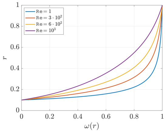
Figure 7. Angular velocity (31) for various $\mathsf{Re}<{\mathsf{\Gamma }}^2$, $\mathsf{\Gamma }=15$, $R_1=0.1$.

2.3. Flow down an Inclined Plane

In this section, we focus on the flow down an inclined plane whose tilt angle with the horizontal direction is $\theta$. We assume that the flow is uniform in the $z^{\ast }$ direction so that ${\mathbf{v}}^{\ast }=(u^{\ast }(x^{\ast },y^{\ast }),v^{\ast }(x^{\ast },y^{\ast }))$, and we denote with $y^{\ast }=h^{\ast }(x^{\ast },t^{\ast })$ the upper free surface. We take a reference system $\{O,x^{\ast },y^{\ast }\}$, where the $x^{\ast }$ axis represents the bottom plane and $y^{\ast }$ its normal direction. Rescaling as in the previous section, and assuming that the flow is driven by gravity, the motion equation is

$$\mathsf{Re}\dot{\mathbf{v}}=-\nabla p+\mathrm{div}\left(\mathbf{S}\right)+{\displaystyle \frac{\mathsf{Re}}{{\mathsf{Fr}}^2}}\left(sin\theta \mathbf{i}-cos\theta \mathbf{j}\right),$$

where

$$\mathsf{Fr}={\displaystyle \frac{U^{\ast }}{\sqrt{g^{\ast }{L}^{\ast }}}}$$

is the Froude number. We suppose that the fluid is surrounded by a motionless ambient gas so that, neglecting the surface tension on $h^{\ast }(x^{\ast },t^{\ast })$, we can write the non-dimensional free boundary conditions as

$${\displaystyle \frac{h_x^2\left(p-S_{11}\right)+2h_x{S}_{12}+\left(p-S_{22}\right)}{\left(1+h_x^2\right)}}=0,\mathrm{on}y=h,$$

(32)

$$S_{12}\left(h_x^2-1\right)+\left(S_{11}-S_{22}\right)h_x=0,\mathrm{on}y=h,$$

(33)

$$v=h_{x}u+h_t,\mathrm{on}y=h.$$

(34)

The first two relations express the continuity of the normal and tangential stresses, respectively (dynamic conditions), while the last is a consequence of the fact that $h(x,t)$ is a material surface (kinematic condition). We look for a solution of the types $\mathbf{v}=u\left(y\right)\mathbf{i}$ and $h=const$, so that $S_{12}=S_{12}\left(y\right)$, $S_{11}=S_{22}=0$ and

$$\left\{\begin{array}{c}0=-{\displaystyle \frac{\partial p}{\partial x}}+{\displaystyle \frac{\partial S_{12}}{\partial y}}+\lambda sin\theta ,\hfill \\ \\ 0=-{\displaystyle \frac{\partial p}{\partial y}}-\lambda cos\theta ,\lambda ={\displaystyle \frac{\mathsf{Re}}{{\mathsf{Fr}}^2}}={\rho }^{\ast }{g}^{\ast }{L}^{\ast }{a}^{\ast }.\hfill \end{array}\right.$$

(35)

The constant $\lambda$ is a material parameter. The dynamic boundary conditions for the stress reduce to $p=0$ (the external pressure is rescaled to zero), $S_{12}=0$ on $y=h$, while the kinematic boundary condition is automatically satisfied. The no-slip conditions on the bottom plane are $u=0$ and $2\mid \mathbf{D}\mid =u_y>0$. Integration of linear momentum yields

$$p=\lambda cos\theta \left(h-y\right),S_{12}=ln\left({\displaystyle \frac{b}{b-u_y}}\right)=\delta \left(h-y\right).$$

(36)

where $\delta =\lambda sin\theta >0$. After some calculation, we find

$$u_y=b\left[1-e^{-\delta (h-y)}\right]<b,$$

(37)

and

$$u\left(y\right)=b\left[y-{\displaystyle \frac{e^{-\delta (h-y)}-e^{-\delta h}}{\delta }}\right]$$

(38)

The thickness h of the fluid is unknown and can be determined by imposing the inlet non-dimensional flux $Q=Q^{\ast }/\left(U^{\ast }{H}^{\ast }\right)$, where $Q^{\ast }$ is the dimensional discharge. Exploiting (38), we have

$$Q={\int }_0^{h}u\left(y\right)dy=b\left[{\displaystyle \frac{h^2}{2}}-{\displaystyle \frac{1-e^{-\delta h}(1+\delta h)}{{\delta }^2}}\right]$$

(39)

Hence, $Q=Q\left(h\right)$ with $Q\left(0\right)=0$, $Q(\infty )=\infty$, $Q^{\prime }=h(1-e^{-\delta h})⩾0$. As a consequence, for any positive given Q, there exists a unique h, satisfying (39). We may select $U^{\ast }$, so that the maximum velocity, which is attained at $y=h$, is equal to one. From (38), setting $u\left(h\right)=1$, we find

$$b={\left[h-{\displaystyle \frac{1-e^{-\delta h}}{\delta }}\right]}^{-1}⟺h={\displaystyle \frac{1}{\delta }}\left[\left(1+{\displaystyle \frac{\delta }{b}}\right)+\mathcal{W}\left(-e^{\left(1+{\displaystyle \frac{\delta }{b}}\right)}\right)\right],$$

(40)

where $\mathcal{W}$ is again the zero branch of the Lambert function. Substituting (40)${}_1$ into (38), we find

$$u\left(y\right)=\left[{\displaystyle \frac{e^{-\delta h}+\delta y-e^{-\delta (h-y)}}{e^{-\delta h}+\delta h-1}}\right].$$

(41)

Recalling that $b=\mathsf{\Gamma }/\sqrt{\mathsf{Re}}$, we finally write the velocity profile for the flow down an inclined plane as

$$\left\{\begin{array}{c}u\left(y\right)=\left[{\displaystyle \frac{e^{-\delta h}+\delta y-e^{-\delta (h-y)}}{e^{-\delta h}+\delta h-1}}\right],\hfill \\ \\ h={\displaystyle \frac{1}{\delta }}\left[\left(1+{\displaystyle \frac{\delta \sqrt{\mathsf{Re}}}{\mathsf{\Gamma }}}\right)+\mathcal{W}\left(-e^{\left(1+{\displaystyle \frac{\delta \sqrt{\mathsf{Re}}}{\mathsf{\Gamma }}}\right)}\right)\right]\hfill \end{array}\right.$$

(42)

In Figure 8 we show the velocity profile (42) for various $\mathsf{Re}$ with $\mathsf{\Gamma }=15$, $\lambda =1.3$ and $\theta =\pi /4$.

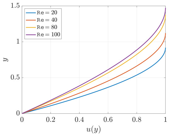
Figure 8. Velocity (42) for various $\mathsf{Re}$, $\mathsf{\Gamma }=15$, $\lambda =1.3$, $\theta =\pi /4$. Flow down an incline.

We observe that, in this case, no limitation on $\mathsf{Re}$ is present. Indeed, from (40), we see that the increase of $\mathsf{Re}$ results in an increase in h, i.e., in practice, the height of the fluid layer can adapt to the imposed discharge.

3. Linear Stability Analysis

In this section, we consider two-dimensional perturbations of the basic solutions determined in the previous sections. In particular, let ${\psi }_b$ denote any of the steady solutions found in the previous sections. We write

$$\psi ={\psi }_b+\widehat{\psi }\left(y\right)e^{i\alpha (x-ct)}$$

(43)

so that $\psi$ is the sum of the basic function ${\psi }_b$ and the perturbation $\widehat{\psi }\left(y\right)e^{i\alpha (x-ct)}$, where $\widehat{\psi }$ is the complex wave amplitude, $\alpha$ is the wavenumber, c is the complex wave velocity, and we assume that $\mid \widehat{\psi }\mid =O\left(\epsilon \right)$, $\epsilon \ll 1$. The stress tensor can be decomposed as

$${\mathbf{S}}_b+\widehat{\mathbf{S}}{e}^{i\alpha (x-ct)}=ln\left[{\displaystyle \frac{b}{b-2\mid {\mathbf{D}}_b+\widehat{\mathbf{D}}{e}^{i\alpha (x-ct)}\mid }}\right]{\displaystyle \frac{\left({\mathbf{D}}_b+\widehat{\mathbf{D}}{e}^{i\alpha (x-ct)}\right)}{\mid \left({\mathbf{D}}_b+\widehat{\mathbf{D}}{e}^{i\alpha (x-ct)}\right)\mid }}.$$

(44)

The above can be linearized (neglecting terms of order $\epsilon$ and higher) to obtain

$$\widehat{\mathbf{S}}=ln\left[{\displaystyle \frac{b}{b-2\mid {\mathbf{D}}_b\mid }}\right]\left[{\displaystyle \frac{\widehat{\mathbf{D}}}{\mid {\mathbf{D}}_b\mid }}-{\displaystyle \frac{({\mathbf{D}}_b·\widehat{\mathbf{D}}){\mathbf{D}}_b}{2\mid {\mathbf{D}}_b{\mid }^3}}\right]+{\displaystyle \frac{({\mathbf{D}}_b·\widehat{\mathbf{D}}){\mathbf{D}}_b}{\mid {\mathbf{D}}_b{\mid }^2\left(b-2\mid {\mathbf{D}}_b\mid \right)}}$$

(45)

so that $\widehat{\mathbf{S}}$ is linear in $\widehat{\mathbf{D}}$.

3.1. Channel Flow

In the two-dimensional setting, we have

$${\widehat{D}}_{11}=-{\widehat{D}}_{22}=-{\widehat{v}}^{\prime },{\widehat{D}}_{12}=-{\displaystyle \frac{1}{2i\alpha }}\left({\widehat{v}}^{\prime \prime }+{\alpha }^2\widehat{v}\right)$$

(46)

In the context of channel flow, we find

$${\widehat{S}}_{11}=-{\widehat{S}}_{22}=-\stackrel{T\left(y\right)}{\overbrace{\left[{\displaystyle \frac{1}{\mid u_b^{\prime }\mid }}ln\left({\displaystyle \frac{b}{b-\mid u_b^{\prime }\mid }}\right)\right]}}2{\widehat{v}}^{\prime }$$

(47)

$${\widehat{S}}_{12}=-\underset{M\left(y\right)}{\underbrace{\left[{\displaystyle \frac{1}{b-\mid u_b^{\prime }\mid }}\right]}}{\displaystyle \frac{({\widehat{v}}^{″}+{\alpha }^2\widehat{v})}{i\alpha }},$$

(48)

where we indicated with $u_b\left(y\right)$ the basic solution (18). The perturbed momentum equation is

$$-\mathsf{Re}[(u_b-c)\left({\widehat{v}}^{″}-{\alpha }^2\widehat{v})-u_b^{″}\widehat{v}\right]=2i\alpha {\widehat{S}}_{11}^{\prime }+{\widehat{S}}_{12}^{″}+{\alpha }^2{\widehat{S}}_{12}.$$

(49)

Substituting (47), (48) into (49), we obtain the perturbation equation for $\widehat{v}$

$$-i\alpha \mathsf{Re}[(u_b-c)\left({\mathsf{D}}^2-{\alpha }^2)-u_b^{″}\right]\widehat{v}=4{\alpha }^2\mathsf{D}\left(T\mathsf{D}\widehat{v}\right)$$

$$-{\mathsf{D}}^2\left[M\left({\mathsf{D}}^2+{\alpha }^2\right)\widehat{v}\right]-{\alpha }^2\left[M\left({\mathsf{D}}^2+{\alpha }^2\right)\widehat{v}\right]$$

(50)

where $M\left(y\right)$ and $T\left(y\right)$ are defined in Equations (47) and (48), respectively. The boundary conditions are $\widehat{v}(\pm 1)=\mathsf{D}\widehat{v}(\pm 1)=0$. Equation (50) is solved via a spectral collocation method based on Chebyshev polynomials. Notice that because of the particular constitutive equation considered here, the classical Orr–Sommerfeld equation cannot be recovered from (50). In Figure 9, we plot the neutral stability curves for some values of $\mathsf{\Gamma }$, while in Figure 10, we display the critical Reynolds number ${\mathsf{Re}}_c$ as a function of the parameter $\mathsf{\Gamma }$. Notice that the critical Reynolds number is always below the limit ${\mathsf{\Gamma }}^2$, which is the upper bound of $\mathsf{Re}$, see Section 2.1. In particular, we observe that the deviation of ${\mathsf{Re}}_c$ from the limit value $\mathsf{Re}={\mathsf{\Gamma }}^2$ increases with $\mathsf{\Gamma }$.

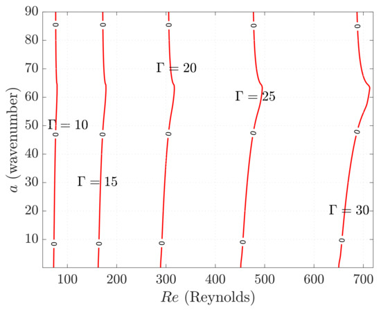
Figure 9. Neutral stability curves in the $(\alpha ,\mathsf{Re})$ plane, channel flow. $\mathsf{\Gamma }=10,15,20,25,30$.

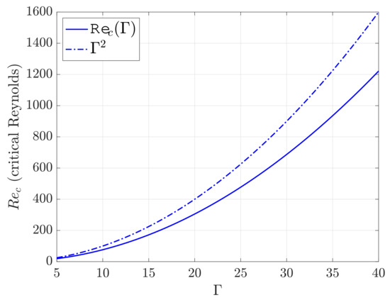
Figure 10. Critical Reynolds number vs. $\mathsf{\Gamma }$: channel flow. Notice that the discrepancy between the ${\mathsf{Re}}_c$ and the upper bound ${\mathsf{\Gamma }}^2$ increases with $\mathsf{\Gamma }$.

3.2. Taylor–Couette Flow

Here, we study the linear stability of the flow between coaxial rotating cylinders. In this case, the perturbed velocity is $\mathbf{v}=v_b\left(r\right){\mathbf{e}}_{\theta }+\widehat{\mathbf{v}}\left(r\right)e^{i\alpha (z-ct)}$, where

$$\widehat{\mathbf{v}}=\widehat{u}{\mathbf{e}}_r+\widehat{v}{\mathbf{e}}_{\theta }+\widehat{w}{\mathbf{e}}_z$$

is the complex amplitude of the perturbation of the velocity, where $v_b\left(r\right)=r{\omega }_b\left(r\right)$ is the basic tangential velocity and where ${\omega }_b\left(r\right)$ is the angular velocity given in (31). We are, thus, considering an axisymmetric perturbation (there is no dependence on the azimuthal coordinate $\theta$). The components of the symmetric part of the perturbation velocity gradient are

$${\widehat{D}}_{rr}={\widehat{u}}^{\prime },{\widehat{D}}_{\theta \theta }={\displaystyle \frac{\widehat{u}}{r}},{\widehat{D}}_{zz}=i\alpha \widehat{w}.$$

(51)

$${\widehat{D}}_{r\theta }={\displaystyle \frac{1}{2}}\left({\widehat{v}}^{\prime }-{\displaystyle \frac{\widehat{v}}{r}}\right),{\widehat{D}}_{rz}={\displaystyle \frac{1}{2}}\left(i\alpha \widehat{u}+{\widehat{w}}^{\prime }\right),{\widehat{D}}_{\theta z}={\displaystyle \frac{i\alpha \widehat{v}}{2}},$$

(52)

where the prime now stands for differentiation with respect to r, i.e., ${}^{\prime }=d/dr$. The linearized momentum equation for the perturbations $(\widehat{u},\widehat{v},\widehat{w})$ are

$$\mathsf{Re}\left[-i\alpha c\widehat{u}-2{\omega }_b\widehat{v}\right]=-\mathsf{\Pi }{\widehat{p}}^{\prime }+{\displaystyle \frac{{\left(r{\widehat{S}}_{rr}\right)}^{\prime }}{r}}-{\displaystyle \frac{{\widehat{S}}_{\theta \theta }}{r}}+i\alpha {\widehat{S}}_{rz}$$

(53)

$$\mathsf{Re}\left[-i\alpha c\widehat{v}+{\displaystyle \frac{{\left(r^2{\omega }_b\right)}^{\prime }}{r}}\widehat{u}\right]={\displaystyle \frac{{\left(r^2{\widehat{S}}_{r\theta }\right)}^{\prime }}{r^2}}+i\alpha {\widehat{S}}_{\theta z}$$

(54)

$$\mathsf{Re}\left[-i\alpha c\widehat{w}\right]=-\mathsf{\Pi }i\alpha \widehat{p}+{\displaystyle \frac{{\left(r{\widehat{S}}_{rz}\right)}^{\prime }}{r}}+i\alpha {\widehat{S}}_{zz}$$

(55)

Multiplying (53) by $-i\alpha$, differentiating (55) with respect to r, and summing up, we have

$$\mathsf{Re}\left[i\alpha \left(2{\omega }_b\widehat{v}-c{\widehat{w}}^{\prime }\right)-{\alpha }^{2}c\widehat{u}\right]=-{\displaystyle \frac{i\alpha }{r}}{\left(r{\widehat{S}}_{rr}\right)}^{\prime }$$

$$-{\displaystyle \frac{1}{r^2}}{\left(r{\widehat{S}}_{rz}\right)}^{\prime }+{\displaystyle \frac{1}{r}}{\left(r{\widehat{S}}_{rz}\right)}^{″}+i\alpha \left({\displaystyle \frac{{\widehat{S}}_{\theta \theta }}{r}}+{\widehat{S}}_{zz}^{\prime }-i\alpha {\widehat{S}}_{rz}\right)$$

(56)

From the continuity equation, we find

$$\widehat{w}={\displaystyle \frac{i}{\alpha }}\left[{\widehat{u}}^{\prime }+{\displaystyle \frac{\widehat{u}}{r}}\right],⟹{\widehat{w}}^{\prime }={\displaystyle \frac{i}{\alpha }}\left({\widehat{u}}^{″}-{\displaystyle \frac{\widehat{u}}{r^2}}+{\displaystyle \frac{{\widehat{u}}^{\prime }}{r}}\right)$$

The linearized constitutive Equation (45) in the cylindrical coordinates becomes

$$\widehat{\mathbf{S}}=ln\left({\displaystyle \frac{b}{b-r{\omega }_b^{\prime }}}\right)\left[{\displaystyle \frac{2\widehat{\mathbf{D}}}{r{\omega }_b^{\prime }}}-{\displaystyle \frac{4{\widehat{D}}_{r\theta }{\mathbf{D}}_b}{{\left(r{\omega }_b^{\prime }\right)}^2}}\right]+{\displaystyle \frac{4{\widehat{D}}_{r\theta }{\mathbf{D}}_b}{r{\omega }_b^{\prime }(b-r{\omega }_b^{\prime })}}$$

(57)

from which we derive

$${\widehat{S}}_{rr}=T\left(r\right)2{\widehat{u}}^{\prime },{\widehat{S}}_{\theta \theta }=T\left(r\right){\displaystyle \frac{2\widehat{u}}{r}},{\widehat{S}}_{zz}=-T\left(r\right)2\left({\widehat{u}}^{\prime }+{\displaystyle \frac{\widehat{u}}{r}}\right)$$

(58)

$${\widehat{S}}_{r\theta }=M\left(r\right)\left({\widehat{v}}^{\prime }-{\displaystyle \frac{\widehat{v}}{r}}\right),{\widehat{S}}_{rz}=T\left(r\right){\displaystyle \frac{i}{\alpha }}\left({\widehat{u}}^{″}-{\displaystyle \frac{\widehat{u}}{r^2}}+{\displaystyle \frac{{\widehat{u}}^{\prime }}{r}}+{\alpha }^2\widehat{u}\right),$$

(59)

$${\widehat{S}}_{\theta z}=T\left(r\right)i\alpha \widehat{v},{\widehat{S}}_{zz}=-T\left(r\right)2\left({\widehat{u}}^{\prime }+{\displaystyle \frac{\widehat{u}}{r}}\right),$$

(60)

where

$$T\left(r\right)={\displaystyle \frac{1}{r{\omega }_b^{\prime }}}ln\left({\displaystyle \frac{b}{b-r{\omega }_b^{\prime }}}\right),M\left(r\right)={\displaystyle \frac{1}{b-r{\omega }_b^{\prime }}}.$$

Inserting (58)–(60) into (54), (56), we finally find the eigenvalue problem

$$c\left[\begin{array}{cc}\mathsf{Re}\left({\mathsf{D}}^2+{\displaystyle \frac{\mathsf{D}}{r}}-{\displaystyle \frac{1}{r^2}}-{\alpha }^2\right)\hfill & \hfill 0\\ \\ 0\hfill & \hfill -\mathsf{Re}i\alpha \end{array}\right]\left[\begin{array}{c}\widehat{u}\\ \\ \widehat{v}\end{array}\right]=-\left[\begin{array}{cc}{\mathcal{L}}_1\hfill & \hfill {\mathcal{M}}_1\\ \\ {\mathcal{L}}_2\hfill & \hfill {\mathcal{M}}_2\end{array}\right]\left[\begin{array}{c}\widehat{u}\\ \\ \widehat{v}\end{array}\right]$$

(61)

where $\mathsf{D}=d/dr$ and where

$${\mathcal{L}}_1=i\left[T\left(-{\displaystyle \frac{2\alpha }{r^2}}+{\displaystyle \frac{3}{\alpha r^4}}-{\alpha }^3\right)+T^{\prime }\left({\displaystyle \frac{\alpha }{r}}-{\displaystyle \frac{3}{\alpha r^3}}\right)+T^{″}\left({\displaystyle \frac{1}{\alpha r^2}}-\alpha \right)\right]+$$

$$i\left[T\left({\displaystyle \frac{2\alpha }{r}}-{\displaystyle \frac{3}{\alpha r^3}}\right)+T^{\prime }\left({\displaystyle \frac{3}{\alpha r^2}}+2\alpha \right)-T^{″}\left({\displaystyle \frac{1}{\alpha r}}\right)\right]\mathsf{D}+$$

$$i\left[T\left({\displaystyle \frac{3}{\alpha r^2}}+2\alpha \right)-T^{\prime }\left({\displaystyle \frac{3}{\alpha r}}\right)-T^{″}\left({\displaystyle \frac{1}{\alpha }}\right)\right]{\mathsf{D}}^2+$$

$$-i\left[T\left({\displaystyle \frac{2}{\alpha r}}\right)+T^{\prime }\left({\displaystyle \frac{2}{\alpha }}\right)\right]{\mathsf{D}}^3-\left[T{\displaystyle \frac{1}{\alpha }}\right]{\mathsf{D}}^4$$

$${\mathcal{M}}_1=2\mathsf{Re}i\alpha {\omega }_b,{\mathcal{L}}_2=\mathsf{Re}\left[r{\omega }_b^{\prime }+2{\omega }_b\right]$$

$${\mathcal{M}}_2=\left[{\displaystyle \frac{M^{\prime }}{r}}+{\displaystyle \frac{M}{r^2}}+{\displaystyle \frac{{\alpha }^2}{r^2}}T\right]-\left[{\displaystyle \frac{M}{r}}+M^{\prime }\right]\mathsf{D}-M{\mathsf{D}}^2$$

The eigenvalue problem is coupled with boundary conditions $\widehat{u}\left(1\right)=\mathsf{D}\widehat{u}\left(1\right)=\widehat{v}\left(1\right)=0$ and $\widehat{u}\left(R_1\right)=\mathsf{D}\widehat{u}\left(R_1\right)=\widehat{v}\left(R_1\right)=0$. Problem (61) is solved by a spectral collocation method based on Chebyshev polynomials (the spatial domain $[R_1,1]$ is mapped in the interval $[-1,1]$). In Figure 11, we plot the neutral stability curves for some values of $\mathsf{\Gamma }$. In Figure 12, we show the critical Reynolds number as a function of the parameter $\mathsf{\Gamma }$. Notice that the critical Reynolds number is always below the limit ${(-\mathsf{\Gamma }ln{R}_1^{-1})}^2$. In particular, we observe that the deviation of ${\mathsf{Re}}_c$ from the limit value $\mathsf{Re}={(-\mathsf{\Gamma }ln{R}_1^{-1})}^2$ increases with $\mathsf{\Gamma }$ as in the channel flow.

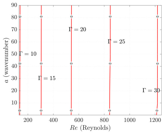
Figure 11. Neutral stability curves, the flow between rotating cylinders. $\mathsf{\Gamma }=10,15,20,25,30$.

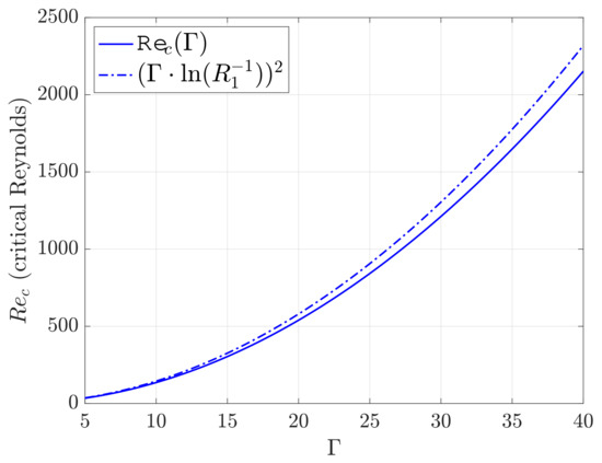
Figure 12. Critical Reynolds number vs. $\mathsf{\Gamma }$: flow between rotating cylinders. Notice again the discrepancy between ${\mathsf{Re}}_c$ and the upper bound as $\mathsf{\Gamma }$ increases.

3.3. Flow down an Inclined Plane

In this section, we study the linear stability of the downhill flow presented in Section 2.3. The perturbed variables are in the form (43) and the equation for the perturbation is still (50), the spatial domain being $[0,h_b]$, with $h_b$ given in (42)${}_2$. Introducing the perturbed free surface

$$h=h_b+\widehat{h}{e}^{i\alpha (x-ct)},\widehat{h}\in \mathbb{C},$$

we check that the linearized boundary conditions (32)–(34) become:

$$\widehat{h}=-{\displaystyle \frac{2b^{-1}{\widehat{v}}^{\prime }\left(h_b\right)-\widehat{p}\left(h_b\right)}{\lambda cos\theta }},$$

(62)

$$\widehat{h}=-{\displaystyle \frac{1}{\delta b}}{\displaystyle \frac{{\widehat{v}}^{″}\left(h_b\right)+{\alpha }^2\widehat{v}\left(h_b\right)}{i\alpha }},$$

(63)

$$\widehat{v}\left(h_b\right)=i\alpha \widehat{h}\left[1-c\right].$$

(64)

The pressure term in (62) can be written in terms of $\widehat{v}$ exploiting the first component of the linearized momentum equation for the perturbation, namely

$$\mathsf{Re}\left({\widehat{v}}^{\prime }(c-u_b)+\widehat{v}{u}_b^{\prime }\right)=-i\alpha \widehat{p}+i\alpha {\widehat{S}}_{11}+{\widehat{S}}_{12}^{\prime },$$

(65)

with ${\widehat{S}}_{11}$, ${\widehat{S}}_{12}$ given by (47), (48). Using (65), and eliminating $\widehat{h}$ from (62), (63) we find that

$$\left({\widehat{v}}^{″}+{\alpha }^2\widehat{v}\right)\left(1-c\right)+\delta b\widehat{v}=0,y=h_b,$$

(66)

$$\left({\widehat{v}}^{‴}+{\alpha }^2\widehat{v}\right)-\left({\widehat{v}}^{″}+{\alpha }^2\widehat{v}\right)\left(i\alpha cot\theta +\delta \right)$$

$$-\widehat{v}\left(4{\alpha }^2+i\alpha b\mathsf{Re}(1-c)\right)=0,y=h_b.$$

(67)

Conditions (66), (67), together with the no-slip conditions

$$\widehat{v}\left(0\right)={\widehat{v}}^{\prime }\left(0\right)=0,$$

(68)

provide the boundary conditions for the perturbation $\widehat{v}$. In conclusion, the eigenvalue problem for the stability of the flow down an inclined plane is given by Equation (50)—in the domain $[0,h_b]$-and the boundary conditions (66)–(68). The complex values of the parameter c that produce a non-trivial solution give the relation between the basic flow and the evolution of the disturbance modes. In particular, when the growth rate of the disturbance $\sigma =\alpha Im\left(c\right)$ is positive, the amplitude of the disturbance becomes unbounded and the system is unstable. Here, we limit our analysis to the so-called long-wave analysis, i.e., we assume that $\alpha \ll 1$, so that the solution can be sought in the form of expansion in powers of $\alpha$,

$$\widehat{v}={\widehat{v}}_o+\alpha {\widehat{v}}_1+{\alpha }^2{\widehat{v}}_2+......,c=c_o+\alpha c_1+{\alpha }^2{c}_2+.......$$

Inserting the expansion above in the eigenvalue problem and grouping the terms of the same order, we obtain a sequence of eigenvalue problems that can be solved iteratively. In particular, it can be proved that the problem at the zero order is given by

$$\left\{\begin{array}{c}{\left[M\left(y\right){\widehat{v}}_o^{″}\right]}^{″}=0,\hfill \\ \\ {\widehat{v}}_o={\widehat{v}}_o^{\prime }=0,y=0\hfill \\ \\ {\widehat{v}}_o^{″}(1-c_o)+\delta b{\widehat{v}}_o=0,y=h_b,\hfill \\ \\ {\widehat{v}}_o^{‴}-\delta {\widehat{v}}_o^{″}=0,y=h_b.\hfill \end{array}\right.$$

(69)

Problem (69)${}_1$ is solved by

$${\widehat{v}}_o=e^{\delta y}-\delta y-1,c_o={\displaystyle \frac{e^{-\delta h_b}\left[(\delta +b)e^{\delta h_b}-b(\delta h_b+1)\right]}{\delta }}$$

(70)

from which we immediately see that $c_o\in \mathbb{R}$. We notice that the general eigenvalue problems (50), (66), (67), (68) are homogeneous, so that the solution is defined up to a multiplicative constant. Following the procedure used in [19], we select such a constant so that $\widehat{v}\left(h_b\right)={\widehat{v}}_o\left(h_b\right)$, implying ${\widehat{v}}_i\left(h_b\right)=0$ for $i=1,2,3,....$. The problem with the first order is, therefore,

$$\left\{\begin{array}{c}i\mathsf{Re}\left[(u_b-c_o){\widehat{v}}_o^{″}-u_b^{″}{\widehat{v}}_o\right]={\left[M\left(y\right){\widehat{v}}_1^{″}\right]}^{″},\hfill \\ \\ {\widehat{v}}_1={\widehat{v}}_1^{\prime }=1,y=0\hfill \\ \\ \left[{\widehat{v}}_1^{″}(1-c_o)+\delta b{\widehat{v}}_1\right]-c_1{\widehat{v}}_o^{″}=0,y=h_b,\hfill \\ \\ \left[{\widehat{v}}_1^{‴}-\delta {\widehat{v}}_1^{″}\right]+\left(i\mathsf{Re}{v}_o^{\prime }(c_o-1)-icot\theta {\widehat{v}}_o^{″}\right)=0,y=h_b,\hfill \\ \\ {\widehat{v}}_1=0,y=h_b.\hfill \end{array}\right.$$

(71)

Integration of (71)${}_1$ gives functions ${\widehat{v}}_1={\widehat{v}}_1(y;A,B,C,D)$ in which the dependencies on the integration constants $A,B,C,D$ are linear. The impositions of the five BCs (71)${}_2$–(71)${}_5$ lead to a linear system whose solution provides the constants $A,B,C,D$, and the eigenvalue $c_1$. The calculation for the determination of the eigenvalue $c_1$ was checked using the symbolic software wx Maxima. We obtain

$$c_1=i{\displaystyle \frac{\left\{(c_o-1)\left[{\delta }^3(B_2{h}_b+B_1-B_5)-2B_4\right]+b\delta \left(B_5\delta -3\right)\right\}}{{\delta }^3(e^{\delta h}-\delta h-1)}}+$$

$$+i{\displaystyle \frac{(c_o-1)B_4\left[{\left(\delta h_b\right)}^2+2(\delta h_b+1)\right]+\delta (1+\delta h_b)(B_3-b{B}_5\delta )}{{\delta }^3{e}^{\delta h}(e^{\delta h}-\delta h-1)}}\in \mathbb{C}$$

(72)

where $B_i$, $i=1,2,3,4,5$ are functions of the parameters b, $h_b$, $\delta$, $\mathsf{Re}$, $cot\theta$, $c_o$. In particular, $B_i$ is a pure real number (the imaginary part is zero), so that $c_1$ is a pure complex number. For the sake of brevity, we did not report their expressions, which are quite lengthy. In the long wavelength expansion, of the first order, we take $c\approx c_o+\alpha c_1$, so that the growth rate of the amplitude disturbance is

$$\sigma =-i\alpha c_1.$$

(73)

Recalling that $h_b=h_b(\mathsf{Re},\mathsf{\Gamma },\delta )$, $b=b(h_b,\delta )$ (see (40)), $\delta =\lambda sin\theta$ we immediately realize that at the first order

$$B_i=B_i(\mathsf{Re},\mathsf{\Gamma },\theta ,\lambda ),⟹c_1(Re,\mathsf{\Gamma },\theta ,\lambda ).$$

and

$$\sigma =\sigma (\alpha ,Re,\mathsf{\Gamma },\theta ,\lambda )=-i\alpha c_1(Re,\mathsf{\Gamma },\theta ,\lambda ).$$

In Figure 13, we plot the approximation of the marginal stability curves (valid for small $\alpha$) $\sigma =0$ for $\theta =\pi /4$, $\lambda =1$ and with $\mathsf{\Gamma }=10,15,20,25,30$. These are clearly vertical straight lines in the plane $(\mathsf{Re},\alpha )$ that provide the critical Reynolds above which we have instability. The dependency of the critical Reynolds number ${\mathsf{Re}}_c$ as a function of $\mathsf{\Gamma }$ is depicted in Figure 14.

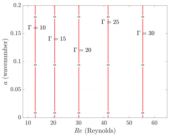
Figure 13. First-order approximation of the neutral stability curves, downhill flow. $\mathsf{\Gamma }=10,15,20,25,30$, $\theta =\pi /4$, $\lambda =1$.

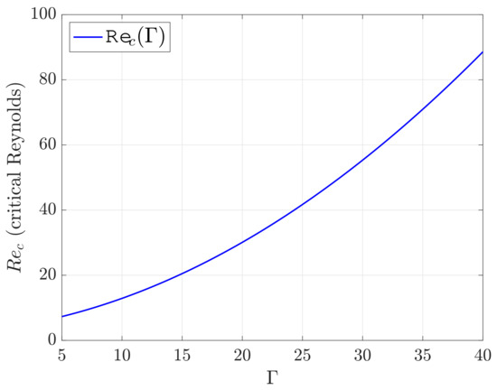
Figure 14. Critical Reynolds number vs. the $\mathsf{\Gamma }$ downhill flow. $\theta =\pi /4$, $\lambda =1$.

As observed in Section 2.3, here we have no limitation of the Reynolds number, since the quantity $b=\mathsf{\Gamma }/\sqrt{\mathsf{Re}}$ is not limited. We notice that the critical Reynolds for the flow down an incline is, in general, much smaller than in the other two cases considered earlier. This is due to the fact that the channel flow and the flow between concentric cylinders are wall-bounded, while the flow down an incline has a free surface. Indeed, it is well known that in the wall-bounded flow, we may have the development of boundary layers that tend to stabilize the flow, see [20]. Furthermore, the discrepancy between the critical Reynolds number of the channel flow (or Taylor–Couette flow) and the flow down an incline is evident even in the case of a Newtonian fluid. For instance, in the channel flow of a Newtonian fluid driven by a pressure drop ${\mathsf{Re}}_c\approx 5700$ (and in the free flow down an incline), the critical Reynolds is given by the relation, see [21]

$${\mathsf{Re}}_c={\displaystyle \frac{5}{4}}cot\theta ,$$

(74)

for an angle of $\pi /4$ (as the one I have considered in the paper) gives ${\mathsf{Re}}_c=1.25$. Finally, we remark that the critical Reynolds numbers for the free surface flow are in the same range as those obtained in [22].

4. Conclusions and Perspectives

We investigated a simple shear flow of a class of dilatant fluids in which the modulus of the deviatoric stress diverges as the modulus of the shear rate tensor tends to a finite positive value. For convenience, these fluids have been termed dilatant fluids with a limited shear rate. The constitutive equation is given by a logarithmic function with two material parameters, $1/a^{\ast }$ and $b^{\ast }$, representing the characteristic apparent viscosity and the shear rate threshold, respectively. The motivation for choosing such a specific form for the apparent viscosity is that it fits (for appropriate values of $a^{\ast }$ and $b^{\ast }$) the flow curves of granular suspensions. The adopted constitutive equation can be viewed as a regularization of a discontinuous shear-thickening constitutive law, such as the one depicted in Figure 1b. Despite the nonlinearity of the apparent viscosity, we are able to determine steady-state solutions for some simple shear flow types. In particular, we considered the (i) planar channel flow, (ii) the flow between concentric cylinders, and (ii) the flow down an inclined plane. In the first two cases, we have shown that the Reynolds number cannot exceed a certain threshold that depends on the material parameters. This seemingly weird behavior is explained; the increase in the velocity automatically increases the resistance opposed to the flow by the increasing viscosity. In this mechanism, the acceptable velocities experienced by the fluid cannot exceed a fixed threshold. In particular, we proved that the limit threshold for the Reynolds number is an increasing function of $a^{\ast }$ and $b^{\ast }$. To investigate the response of the basic steady-state flow to disturbances, we also performed a two-dimensional modal stability analysis for each of the three simple flow types considered. In cases (i) and (ii), the corresponding eigenvalue problems were solved by means of a spectral collocation method based on Chebyshev polynomials, allowing us to plot the neutral stability curves and detect the critical Reynolds number. For the case of the flow down an inclined plane, we limited our analysis to long-wave disturbances (i.e., small wave numbers), explicitly determining the critical Reynolds number. For the three simple shear flow types considered, we found that the critical Reynolds number is an increasing function of $a^{\ast }$ and $b^{\ast }$. This proves that when the limit shear rate threshold is increased, or when the apparent viscosity is decreased, the fluid can be stable for a larger range of Reynolds numbers.

A natural continuation of this work would be (i) the extension to some other simple shear flow; (ii) the analysis of the flow in small-aspect ratio geometries (e.g., lubrication flow); (iii) the investigation of the effects of three-dimensional disturbances and the verification of the validity of Squire’s theorem, which is not automatically valid for non-Newtonian flow. All of these issues are currently under investigation and will be the subject of a forthcoming paper.

References

- Metzner, A.; Whitlock, M. Flow behavior of concentrated (dilatant) suspensions. Trans. Soc. Rheol. 1958, 2, 239–254. [Google Scholar] [CrossRef]
- Sidaoui, N.; Arenas Fernandez, P.; Bossis, G.; Volkova, O.; Meloussi, M.; Aguib, S.; Kuzhir, P. Discontinuous shear thickening in concentrated mixtures of isotropic-shaped and rod-like particles tested through mixer type rheometry. J. Rheol. 2020, 64, 817–836. [Google Scholar] [CrossRef]
- Thomas, J.E.; Goyal, A.; Singh Bedi, D.; Singh, A.; Del Gado, E.; Chakraborty, B. Investigating the nature of discontinuous shear thickening: Beyond a mean-field description. J. Rheol. 2020, 64, 329–341. [Google Scholar] [CrossRef]
- Farina, A.; Fasano, A.; Fusi, L.; Rajagopal, K. The one-dimensional flow of a fluid with limited strain-rate. Q. Appl. Math. 2011, 69, 549–568. [Google Scholar] [CrossRef]
- Mari, R.; Seto, R.; Morris, J.F.; Denn, M.M. Shear thickening, frictionless and frictional rheologies in non-Brownian suspensions. J. Rheol. 2014, 58, 1693–1724. [Google Scholar] [CrossRef]
- Clavaud, C.; Bérut, A.; Metzger, B.; Forterre, Y. Revealing the frictional transition in shear-thickening suspensions. Proc. Natl. Acad. Sci. USA 2017, 114, 5147–5152. [Google Scholar] [CrossRef]
- Singh, A.; Mari, R.; Denn, M.M.; Morris, J.F. A constitutive model for simple shear of dense frictional suspensions. J. Rheol. 2018, 62, 457–468. [Google Scholar] [CrossRef]
- Wyart, M.; Cates, M.E. Discontinuous shear thickening without inertia in dense non-Brownian suspensions. Phys. Rev. Lett. 2014, 112, 098302. [Google Scholar] [CrossRef] [PubMed]
- Brown, E.; Zhang, H.; Forman, N.A.; Maynor, B.W.; Betts, D.E.; DeSimone, J.M.; Jaeger, H.M. Shear thickening and jamming in densely packed suspensions of different particle shapes. Phys. Rev. E 2011, 84, 031408. [Google Scholar] [CrossRef] [PubMed]
- Chhabra, R.; Richardson, J. Non-Newtonian Flow in Process Industries 1999; Biddles Ltd.: Guildford, UK; King’s Lynn, UK, 1999. [Google Scholar]
- Ancey, C. Plasticity and geophysical flow: A review. J. Non-Newton. Fluid Mech. 2007, 142, 4–35. [Google Scholar] [CrossRef]
- Lee, Y.S.; Wetzel, E.D.; Wagner, N.J. The ballistic impact characteristics of Kevlar® woven fabrics impregnated with a colloidal shear thickening fluid. J. Mater. Sci. 2003, 38, 2825–2833. [Google Scholar] [CrossRef]
- Gálvez, L.O.; de Beer, S.; van der Meer, D.; Pons, A. Dramatic effect of fluid chemistry on cornstarch suspensions: Linking particle interactions to macroscopic rheology. Phys. Rev. E 2017, 95, 030602. [Google Scholar]
- Blechta, J.; Málek, J.; Rajagopal, K. On the classification of incompressible fluids and a mathematical analysis of the equations that govern their motion. SIAM J. Math. Anal. 2020, 52, 1232–1289. [Google Scholar] [CrossRef]
- Rajagopal, K.R. On implicit constitutive theories. Appl. Math. 2003, 48, 279–319. [Google Scholar] [CrossRef]
- Ozturk, D.; Morgan, M.L.; Sandnes, B. Flow-to-fracture transition and pattern formation in a discontinuous shear thickening fluid. Commun. Phys. 2020, 3, 119. [Google Scholar] [CrossRef]
- Fusi, L.; Saccomandi, G.; Rajagopal, K.R.; Vergori, L. Flow past a porous plate of non-Newtonian fluids with implicit shear stress shear rate relationships. Eur. J. Mech.-B/Fluids 2022, 92, 166–173. [Google Scholar] [CrossRef]
- Corless, R.M.; Gonnet, G.H.; Hare, D.E.; Jeffrey, D.J.; Knuth, D.E. On the LambertW function. Adv. Comput. Math. 1996, 5, 329–359. [Google Scholar] [CrossRef]
- Pascal, J. Linear stability of fluid flow down a porous inclined plane. J. Phys. D Appl. Phys. 1999, 32, 417. [Google Scholar] [CrossRef]
- Nouar, C.; Frigaard, I. Stability of plane Couette–Poiseuille flow of shear-thinning fluid. Phys. Fluids 2009, 21, 064104. [Google Scholar] [CrossRef]
- Yih, C.S. Stability of liquid flow down an inclined plane. Phys. Fluids 1963, 6, 321–334. [Google Scholar] [CrossRef]
- Darbois Texier, B.; Lhuissier, H.; Forterre, Y.; Metzger, B. Surface-wave instability without inertia in shear-thickening suspensions. Commun. Phys. 2020, 3, 232. [Google Scholar] [CrossRef]
Disclaimer/Publisher’s Note: The statements, opinions and data contained in all publications are solely those of the individual author(s) and contributor(s) and not of MDPI and/or the editor(s). MDPI and/or the editor(s) disclaim responsibility for any injury to people or property resulting from any ideas, methods, instructions or products referred to in the content. |
© 2023 by the author. Licensee MDPI, Basel, Switzerland. This article is an open access article distributed under the terms and conditions of the Creative Commons Attribution (CC BY) license (https://creativecommons.org/licenses/by/4.0/).