
Dynamical Filtering Highlights the Seasonality of Surface-Balanced Motions at Diurnal Scales in the Eastern Boundary Currents


Abstract
1. Introduction
2. Data and Methods
2.1. LLC4320
2.2. Software for Data Processing
- 1.
- Download hourly snapshots for each variable, area and season.
- 2.
- Combine hourly data into time series for each variable and season, and the merge all variables into a single dataset per season and area.
- 3.
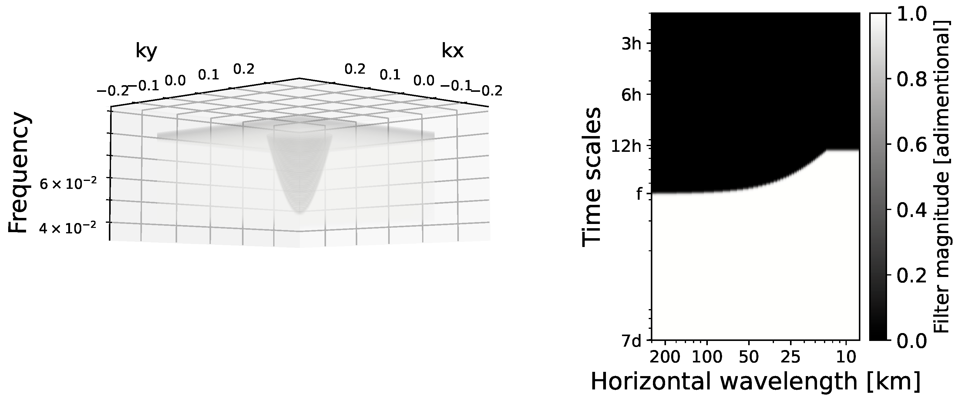
- Calculate dynamical filter in 3D spectral space.
- 4.
- Apply dynamical filter to each variable of interest, namely horizontal components of the ocean surface speed, from which one will obtain the low-pass (balanced motions) and high-pass (internal gravity waves) components.
- 5.
- Compute derived quantities (i.e., and ) for further analyses.
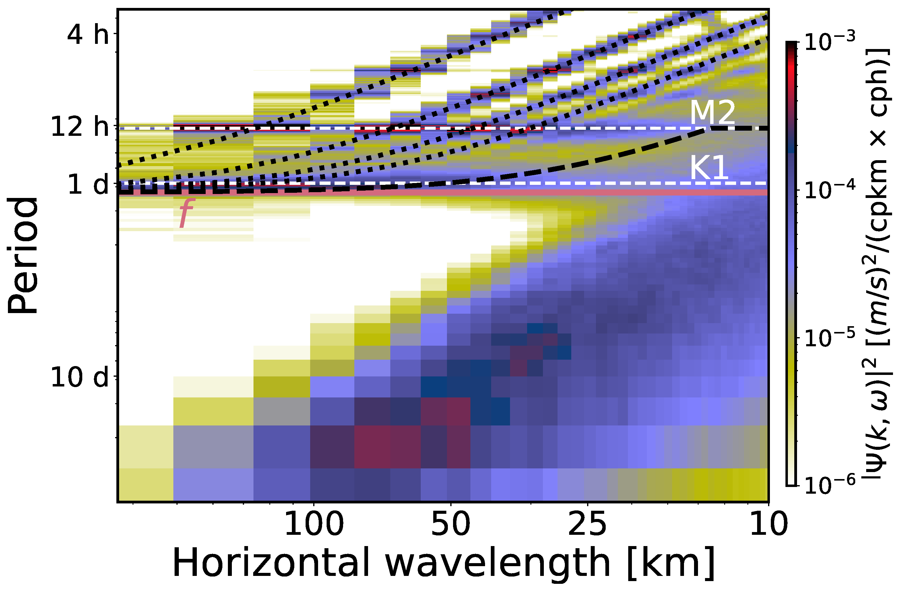
2.3. Spectrum
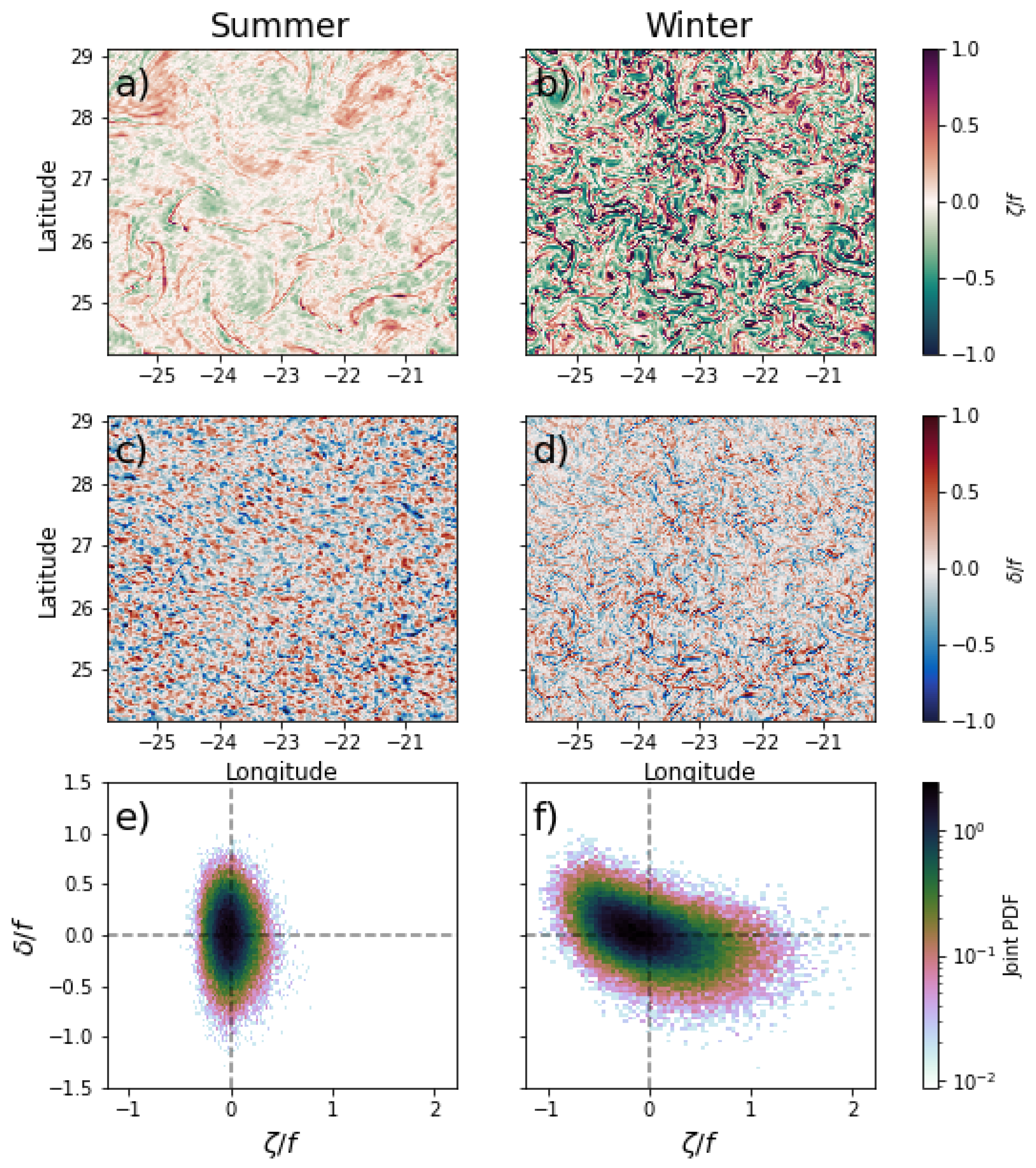
2.4. Temporal Variability of the Vorticity and Divergence Fields
2.5. A Dynamical Filter to Discriminate BM from IGW
Coherence and Phase Difference between Average Intensities of Divergence and Vorticity
3. Results
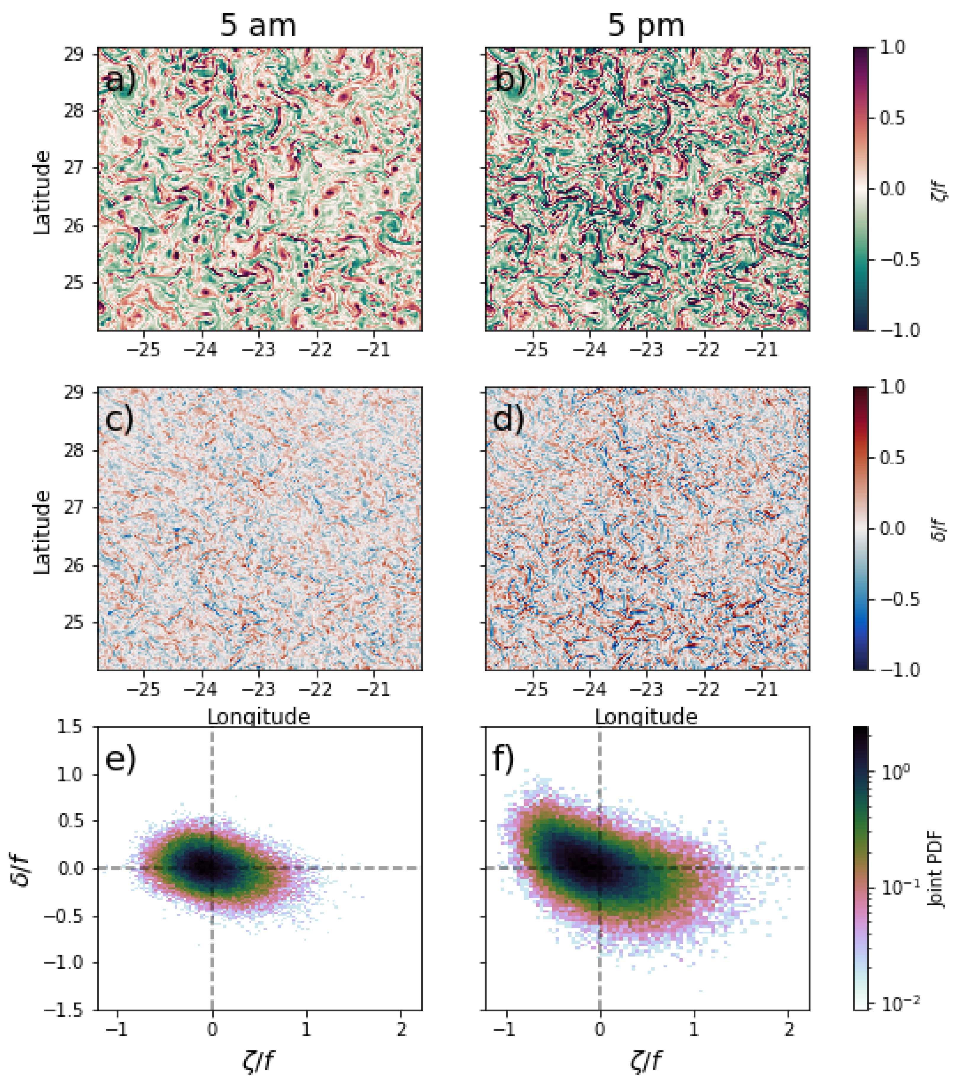
3.1. Comparing and at Seasonal and Diurnal Time Frames
3.2. Rotational-Divergent Ratio in the Frequency–Wavenumber Space
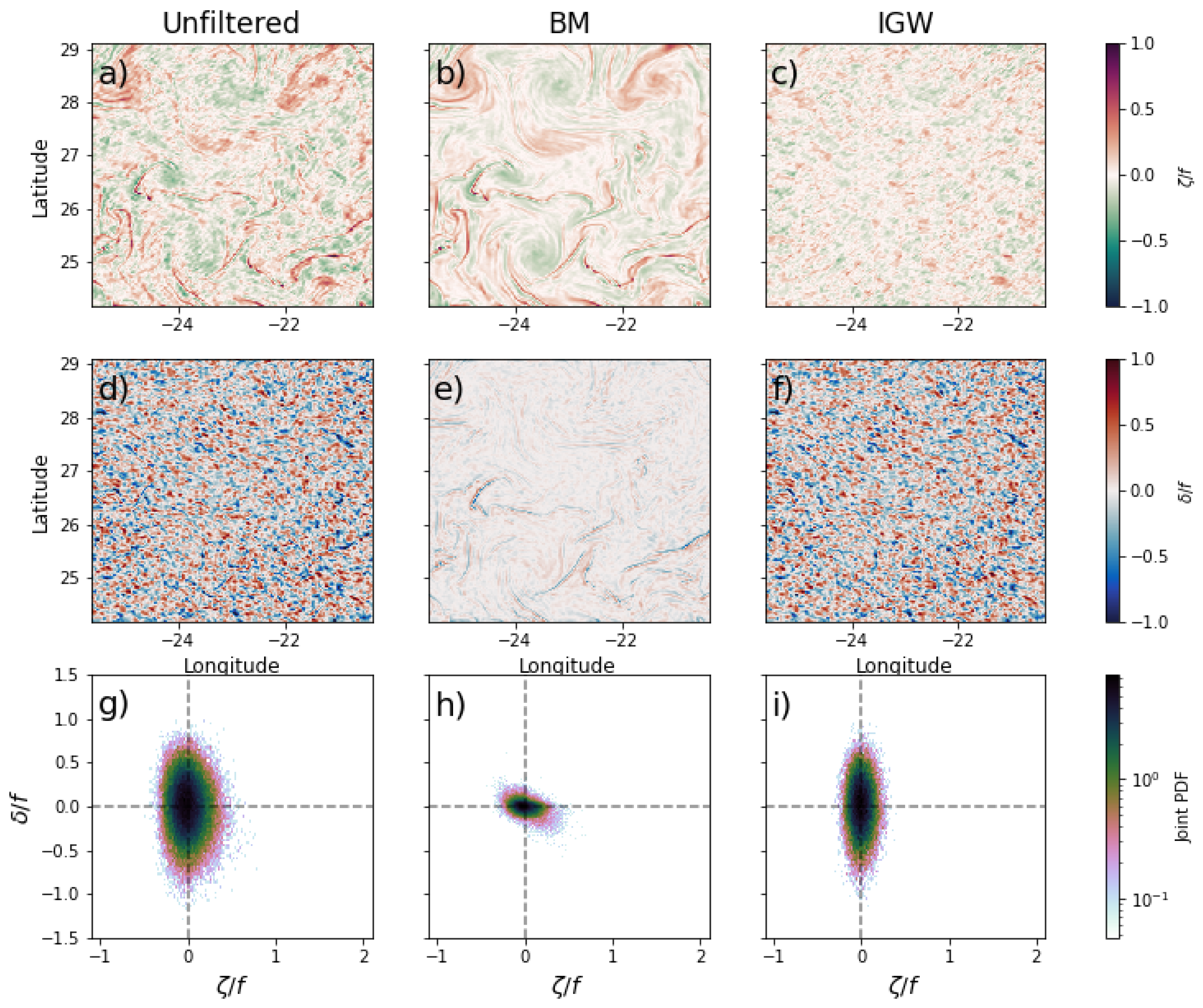
3.3. Separating IGW and BM
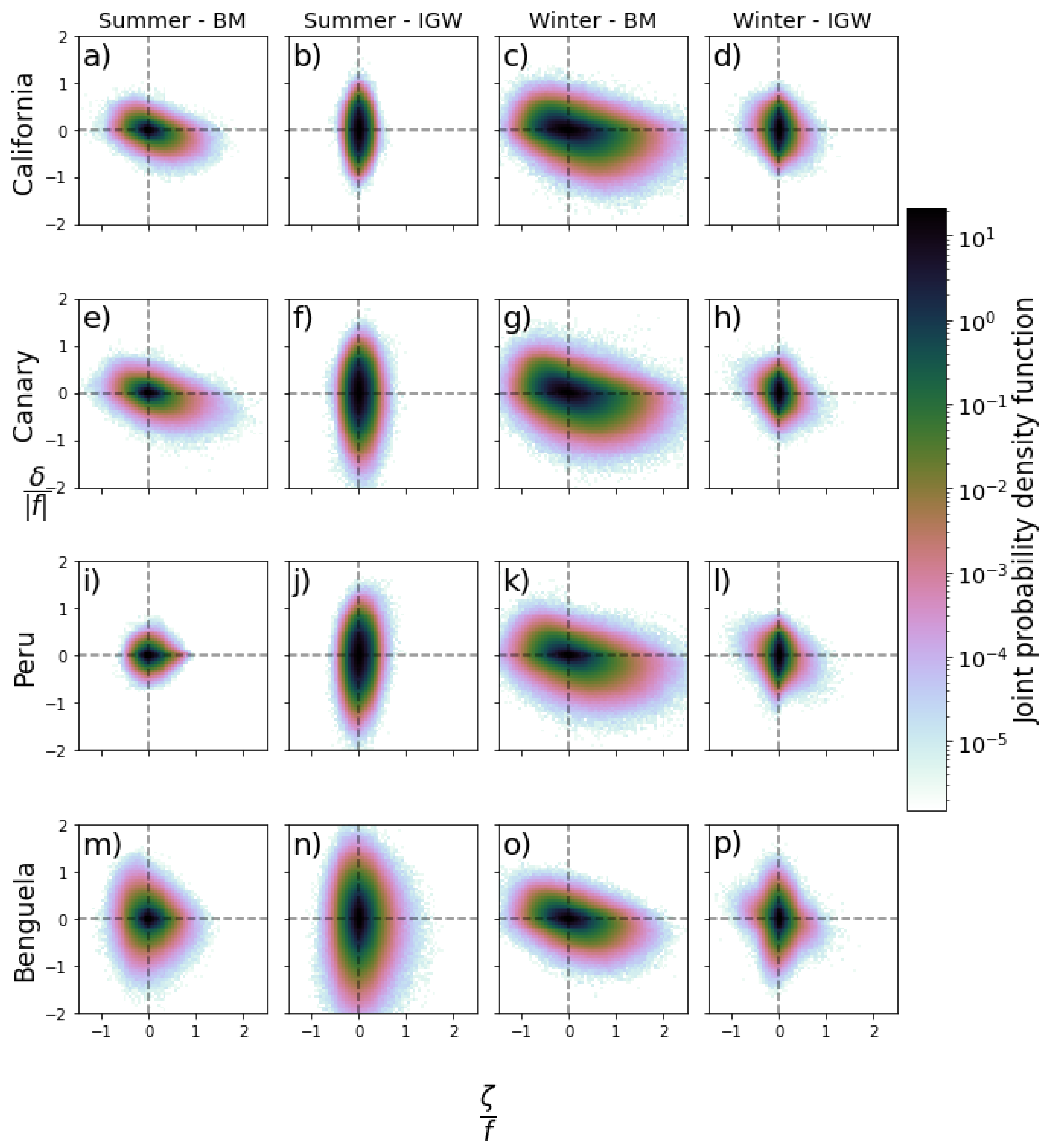
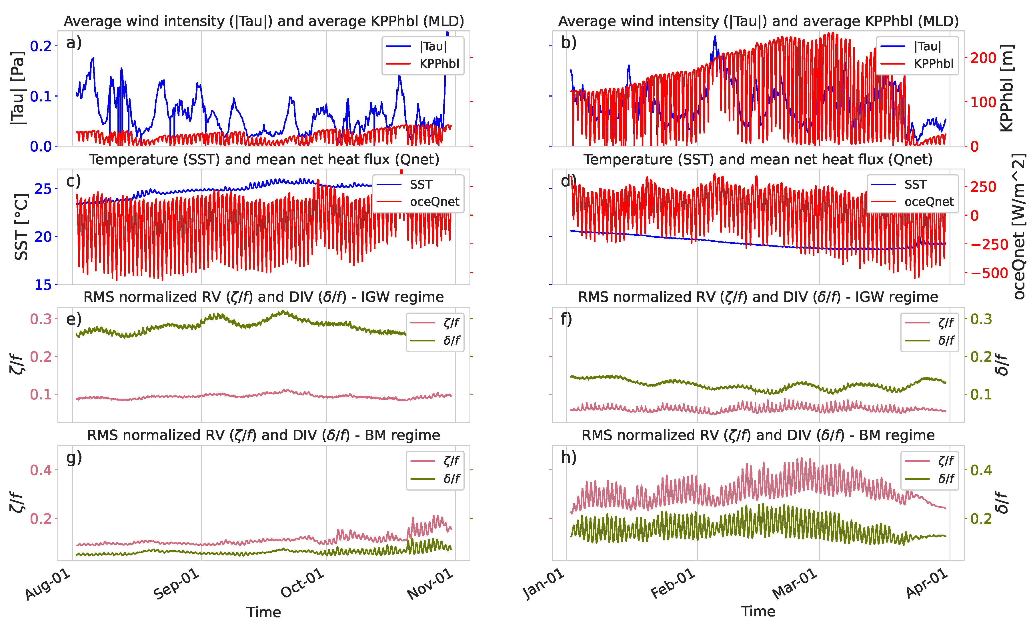
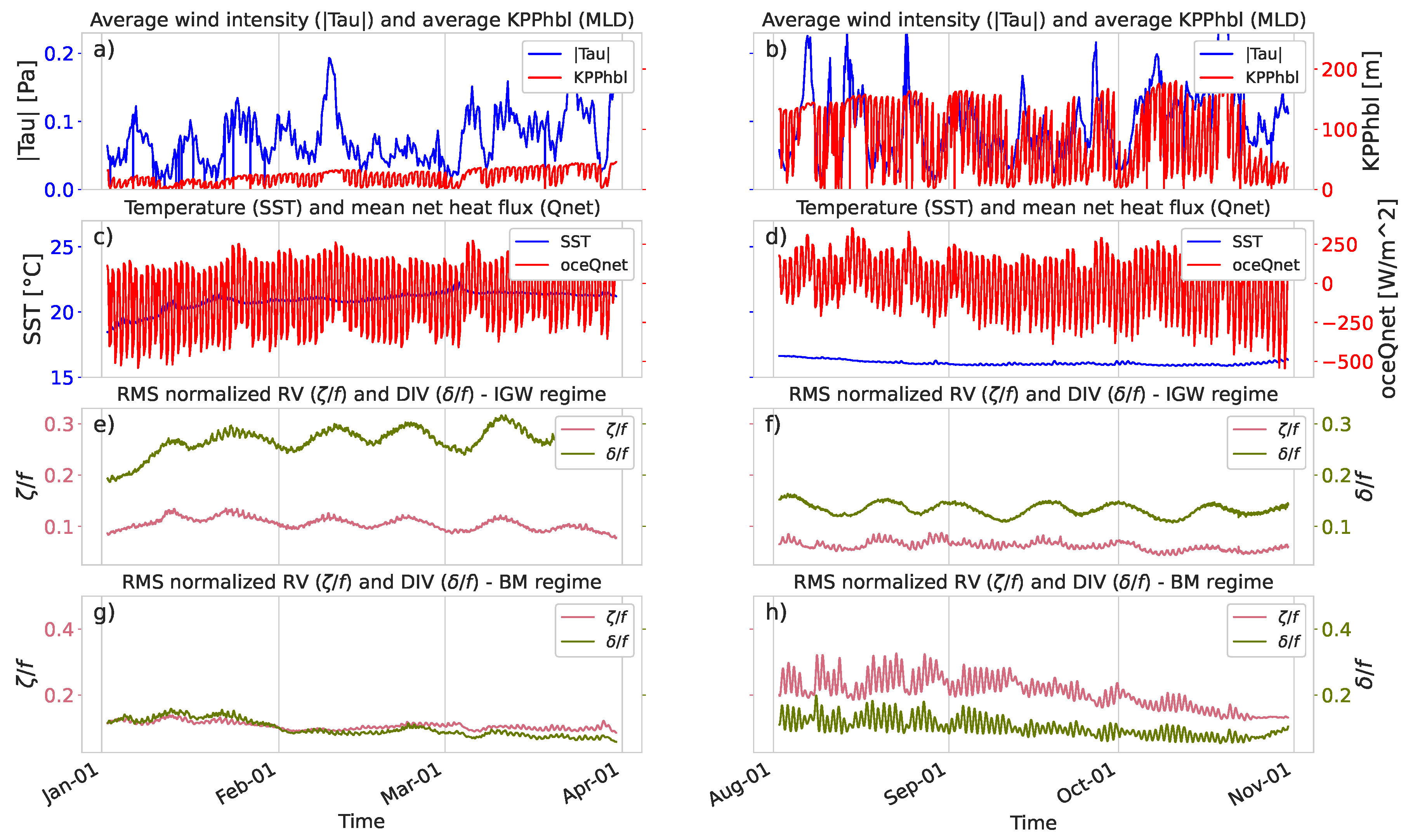
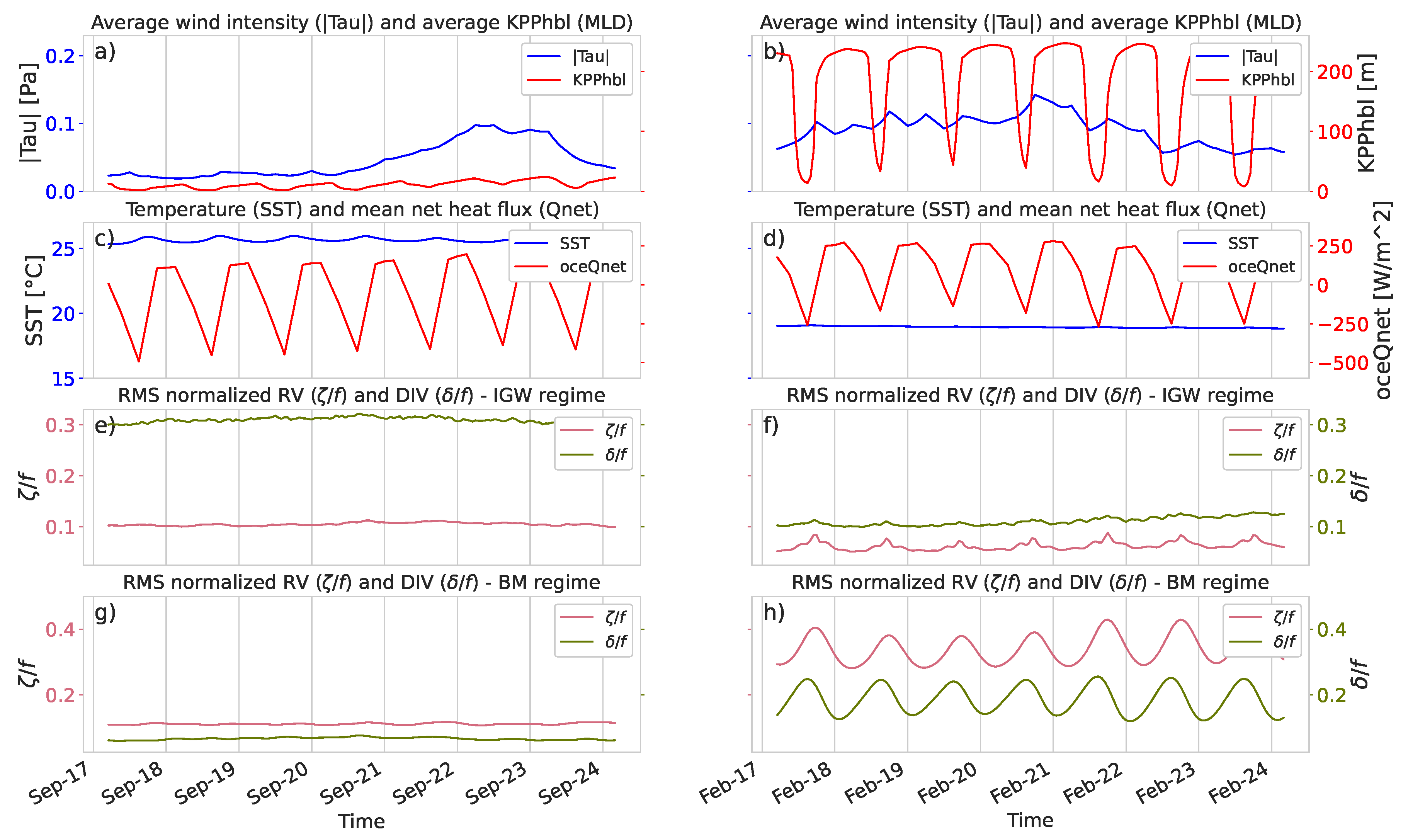
3.4. Seasonal and Diurnal Variability of BM and IGW
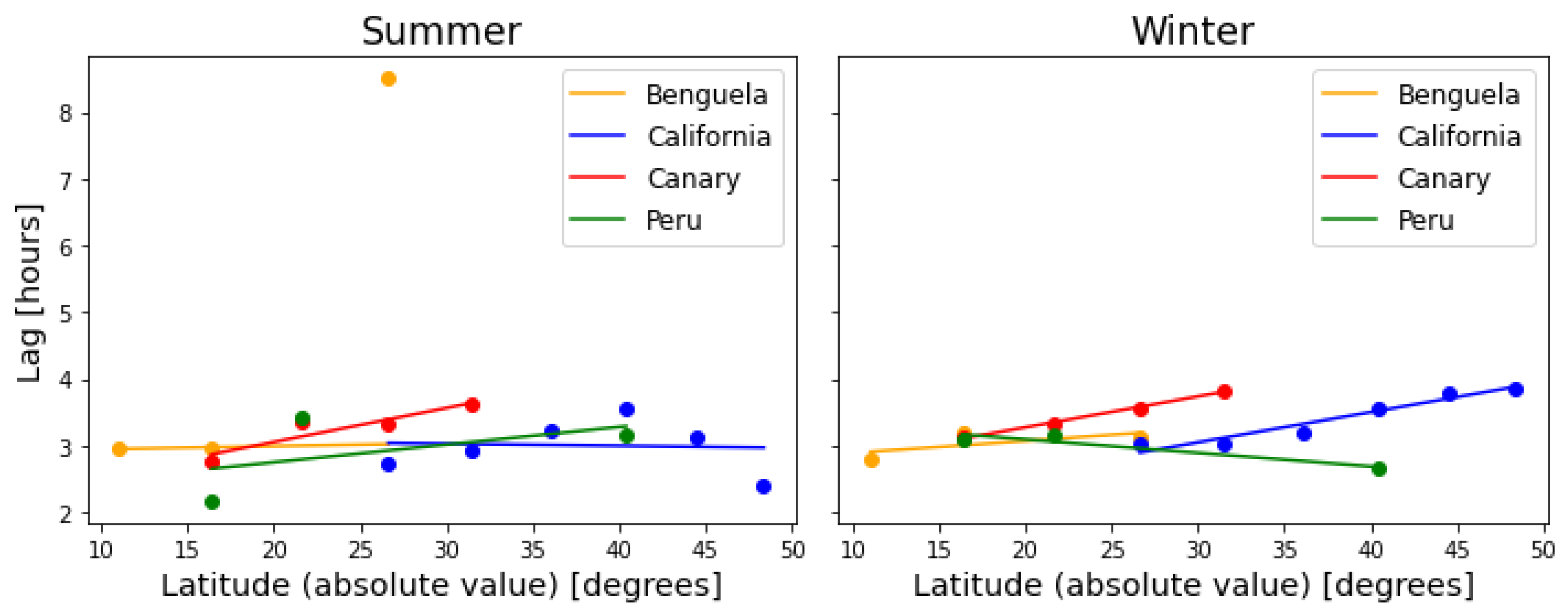
3.5. Diurnal Lag between Divergence and Vorticity
4. Discussion
5. Conclusions and Perspectives
Author Contributions
Funding
Data Availability Statement
Acknowledgments
Conflicts of Interest
Abbreviations
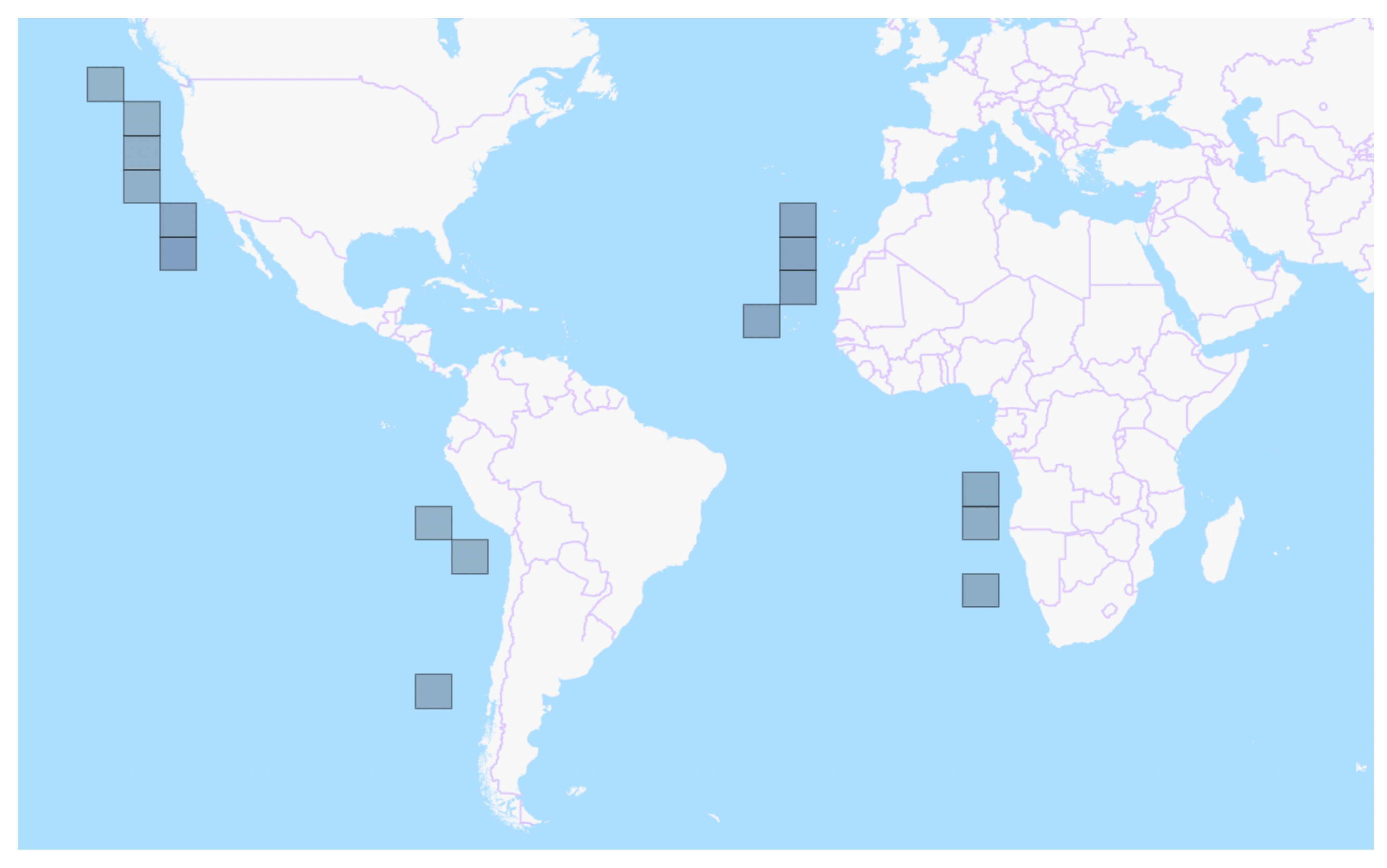
| EBC | Eastern Boundary Current |
| BM | Balanced motions (regime) |
| SBM | Submesoscale balanced motions (regime) |
| IGW | Internal gravity waves (regime) |
| KE | Kinetic energy |
| SSH | Surface sea height |
| FFT | Fast Fourier Transform |
| LLC4320 | MITgcm general circulation model (MITgcm) on a 1/48 nominal Lat/Lon-Cap (LLC) |
| numerical grid | |
| MITgcm | Massachusetts Institute of Technology 55 general circulation model |
| RV | Vertical component of the relative vorticity (also ) |
| DIV | Horizontal divergence (also ) |
| ASO | August–September–October months |
| JFM | January–February–March months |
| NASA | National Aeronautics and Space Administration |
| SWOT | Surface Water and Ocean Topography (satellite mission) |
| S-MODE | Sub-Mesoscale Ocean Dynamics Experiment |
| TTTW | Transient turbulent thermal wind balance |
References
- Cubillos, L.; Núñez, S.; Arcos, D. Producción primaria requerida para sustentar el desembarque de peces pelágicos en Chile. Investig. Mar. 1998, 26, 83–96. [Google Scholar] [CrossRef][Green Version]
- Checkley, D.M.; Barth, J.A. Patterns and processes in the California Current System. Prog. Oceanogr. 2009, 83, 49–64, Eastern Boundary Upwelling Ecosystems: Integrative and Comparative Approaches. [Google Scholar] [CrossRef]
- Chereskin, T.K.; Price, J.F. Ekman Transport and Pumping. In Encyclopedia of Ocean Sciences, 2nd ed.; Academic Press: Cambridge, MA, USA, 2008; pp. 222–227. [Google Scholar] [CrossRef]
- Thomas, A.C.; Strub, P.T.; Carr, M.E.; Weatherbee, R. Comparisons of chlorophyll variability between the four major global eastern boundary currents. Int. J. Remote Sens. 2004, 25, 1443–1447. [Google Scholar] [CrossRef]
- Torres, H.S.; Klein, P.; Menemenlis, D.; Qiu, B.; Su, Z.; Wang, J.; Chen, S.; Fu, L.L. Partitioning Ocean Motions Into Balanced Motions and Internal Gravity Waves: A Modeling Study in Anticipation of Future Space Missions. J. Geophys. Res. Ocean. 2018, 123, 8084–8105. [Google Scholar] [CrossRef]
- Samelson, R.M. Time-Dependent Linear Theory for the Generation of Poleward Undercurrents on Eastern Boundaries. J. Phys. Oceanogr. 2017, 47, 3037–3059. [Google Scholar] [CrossRef]
- Hill, A.E.; Hickey, B.M.; Shillington, F.A.; Strub, P.T.; Brink, K.H.; Barton, E.D.; Thomas, A.C. Eastern Ocean Boundaries, Coastal Segment (E). In The Sea: The Global Coastal Ocean: Regional Studies and Syntheses; Robinson, A.R., Brink, K.H., Eds.; Harvard University Press: Boston, MA, USA, 1998; Volume 11, pp. 29–67. [Google Scholar]
- Barton, E.; Arístegui, J.; Tett, P.; Cantón, M.; García-Braun, J.; Hernández-León, S.; Nykjaer, L.; Almeida, C.; Almunia, J.; Ballesteros, S.; et al. The transition zone of the Canary Current upwelling region. Prog. Oceanogr. 1998, 41, 455–504. [Google Scholar] [CrossRef]
- Klein, P.; Lapeyre, G.; Siegelman, L.; Qiu, B.; Fu, L.L.; Torres, H.; Su, Z.; Menemenlis, D.; Le Gentil, S. Ocean-Scale Interactions from Space. Earth Space Sci. 2019, 6, 795–817. [Google Scholar] [CrossRef]
- Arbic, B.K.; Scott, R.B.; Flierl, G.R.; Morten, A.J.; Richman, J.G.; Shriver, J.F. Nonlinear cascades of surface oceanic geostrophic kinetic energy in the frequency domain. J. Phys. Oceanogr. 2012, 42, 1577–1600. [Google Scholar] [CrossRef]
- Polzin, K.L. Mesoscale Eddy-Internal Wave Coupling. Part II: Energetics and Results from PolyMode. J. Phys. Oceanogr. 2010, 40, 789–801. [Google Scholar] [CrossRef]
- Thomas, L.N.; Ferrari, R. Friction, Frontogenesis, and the Stratification of the Surface Mixed Layer. J. Phys. Oceanogr. 2008, 38, 2501–2518. [Google Scholar] [CrossRef]
- Su, Z.; Torres, H.; Klein, P.; Thompson, A.F.; Siegelman, L.; Wang, J.; Menemenlis, D.; Hill, C. High-Frequency Submesoscale Motions Enhance the Upward Vertical Heat Transport in the Global Ocean. J. Geophys. Res. Ocean. 2020, 125, e2020JC016544. [Google Scholar] [CrossRef]
- Balwada, D.; Smith, K.S.; Abernathey, R. Submesoscale Vertical Velocities Enhance Tracer Subduction in an Idealized Antarctic Circumpolar Current. Geophys. Res. Lett. 2018, 45, 9790–9802. [Google Scholar] [CrossRef]
- Torres, H.S.; Klein, P.; D’Asaro, E.; Wang, J.; Thompson, A.F.; Siegelman, L.; Menemenlis, D.; Rodriguez, E.; Wineteer, A.; Perkovic-Martin, D. Separating Energetic Internal Gravity Waves and Small-Scale Frontal Dynamics. Geophys. Res. Lett. 2022, 49, e2021GL096249. [Google Scholar] [CrossRef]
- Wang, J.; Fu, L.L.; Torres, H.S.; Chen, S.; Qiu, B.; Menemenlis, D. On the Spatial Scales to be Resolved by the Surface Water and Ocean Topography Ka-Band Radar Interferometer. J. Atmos. Ocean. Technol. 2019, 36, 87–99. [Google Scholar] [CrossRef]
- Rocha, C.B.; Gille, S.T.; Chereskin, T.K.; Menemenlis, D. Seasonality of Submesoscale Dynamics in the Kuroshio Extension. Geophys. Res. Lett. 2016, 43, 11304–11311. [Google Scholar] [CrossRef]
- Qiu, B.; Chen, S.; Klein, P.; Wang, J.; Torres, H.; Fu, L.L.; Menemenlis, D.; Qiu, B.; Chen, S.; Klein, P.; et al. Seasonality in Transition Scale from Balanced to Unbalanced Motions in the World Ocean. J. Phys. Oceanogr. 2018, 48, 591–605. [Google Scholar] [CrossRef]
- Chereskin, T.K.; Rocha, C.B.; Gille, S.T.; Menemenlis, D.; Passaro, M. Characterizing the Transition From Balanced to Unbalanced Motions in the Southern California Current. J. Geophys. Res. Ocean. 2019, 124, 2088–2109. [Google Scholar] [CrossRef]
- Dauhajre, D.P.; McWilliams, J.C. Diurnal Evolution of Submesoscale Front and Filament Circulations. J. Phys. Oceanogr. 2018, 48, 2343–2361. [Google Scholar] [CrossRef]
- Siegelman, L.; Klein, P.; Rivière, P.; Thompson, A.F.; Torres, H.; Flexas, M.; Menemenlis, D. Enhanced upward heat transport at deep submesoscale ocean fronts. Nat. Geosci. 2020, 13, 50–55. [Google Scholar] [CrossRef]
- Welch, P.D. The Use of Fast Fourier Transform for the Estimation of Power Spectra: A Method Based on Time Averaging Over Short, Modified Periodograms. IEEE Trans. Audio Electroacoust. 1967, 15, 70–73. [Google Scholar] [CrossRef]
- Flexas, M.M.; Thompson, A.F.; Torres, H.S.; Klein, P.; Farrar, J.T.; Zhang, H.; Menemenlis, D. Global Estimates of the Energy Transfer From the Wind to the Ocean, with Emphasis on Near-Inertial Oscillations. J. Geophys. Res. Ocean. 2019, 124, 5723–5746. [Google Scholar] [CrossRef] [PubMed]
- Pinker, R.T.; Bentamy, A.; Katsaros, K.B.; Ma, Y.; Li, C. Estimates of Net Heat Fluxes over the Atlantic Ocean. J. Geophys. Res. Ocean. 2014, 119, 410–427. [Google Scholar] [CrossRef]
- Erickson, Z.K.; Thompson, A.F.; Callies, J.; Yu, X.; Garabato, A.N.; Klein, P. The Vertical Structure of Open-Ocean Submesoscale Variability during a Full Seasonal Cycle. J. Phys. Oceanogr. 2020, 50, 145–160. [Google Scholar] [CrossRef]
- Quintana, A. Antonimmo/ebc-wk-Spectral-Analysis: V1.2.0. 2022. Available online: https://github.com/antonimmo/ebc-wk-spectral-analysis/tree/1.2.0 (accessed on 5 May 2022).
- Shcherbina, A.Y.; D’Asaro, E.A.; Lee, C.M.; Klymak, J.M.; Molemaker, M.J.; McWilliams, J.C. Statistics of Vertical Vorticity, Divergence, and Strain in a Developed Submesoscale Turbulence Field. Geophys. Res. Lett. 2013, 40, 4706–4711. [Google Scholar] [CrossRef]
- Biltoft, C.A.; Pardyjak, E.R. Spectral Coherence and the Statistical Significance of Turbulent Flux Computations. J. Atmos. Ocean. Technol. 2009, 26, 403–410. [Google Scholar] [CrossRef]
- Capet, X.; McWilliams, J.C.; Molemaker, M.J.; Shchepetkin, A.F. Mesoscale to submesoscale transition in the California Current system. Part II: Frontal processes. J. Phys. Oceanogr. 2008, 38, 44–64. [Google Scholar] [CrossRef]
- Savage, A.C.; Arbic, B.K.; Alford, M.H.; Ansong, J.K.; Farrar, J.T.; Menemenlis, D.; O’Rourke, A.K.; Richman, J.G.; Shriver, J.F.; Voet, G.; et al. Spectral decomposition of internal gravity wave sea surface height in global models. J. Geophys. Res. Ocean. 2017, 122, 7803–7821. [Google Scholar] [CrossRef]
- Garrett, C.J.R.; Loder, J.W. Dynamical aspects of shallow sea fronts. Philos. Trans. R. Soc. Lond. Ser. A Math. Phys. Sci. 1981, 302, 563–581. [Google Scholar] [CrossRef]
- Dauhajre, D.P.; McWilliams, J.C.; Uchiyama, Y.; Dauhajre, D.P.; McWilliams, J.C.; Uchiyama, Y. Submesoscale Coherent Structures on the Continental Shelf. J. Phys. Oceanogr. 2017, 47, 2949–2976. [Google Scholar] [CrossRef]
- Large, W.G.; McWilliams, J.C.; Doney, S.C. Oceanic vertical mixing: A review and a model with a nonlocal boundary layer parameterization. Rev. Geophys. 1994, 32, 363–403. [Google Scholar] [CrossRef]
- Hoskins, B.J.; Bretherton, F.P. Atmospheric Frontogenesis Models: Mathematical Formulation and Solution. J. Atmos. Sci. 1972, 29, 11–37. [Google Scholar] [CrossRef]
- Ferrari, R.; Wunsch, C. Ocean Circulation Kinetic Energy: Reservoirs, Sources, and Sinks. Annu. Rev. Fluid Mech. 2009, 41, 253–282. [Google Scholar] [CrossRef]
- Feliks, Y.; Tziperman, E.; Farrell, B. Nonnormal Frontal Dynamics. J. Atmos. Sci. 2010, 7, 1218–1231. [Google Scholar] [CrossRef]
- Nelson, A.D.; Arbic, B.K.; Zaron, E.D.; Savage, A.C.; Richman, J.G.; Buijsman, M.C.; Shriver, J.F. Toward realistic nonstationarity of semidiurnal baroclinic tides in a hydrodynamic model. J. Geophys. Res. Ocean. 2019, 104, 6632–6642. [Google Scholar] [CrossRef]
- Richards, K.J.; Whitt, D.B.; Brett, G.; Bryan, F.O.; Feloy, K.; Long, M.C. The Impact of Climate Change on Ocean Submesoscale Activity. J. Geophys. Res. Ocean. 2021, 126, e2020JC016750. [Google Scholar] [CrossRef]
- McWilliams, J.C. A Perspective on the Legacy of Edward Lorenz. Earth Space Sci. 2019, 6, 336–350. [Google Scholar] [CrossRef]
- Sun, D.; Bracco, A.; Barkan, R.; Berta, M.; Dauhajre, D.; Molemaker, M.J.; Choi, J.; Liu, G.; Griffa, A.; McWilliams, J.C. Diurnal Cycling of Submesoscale Dynamics: Lagrangian Implications in Drifter Observations and Model Simulations of the Northern Gulf of Mexico. J. Phys. Oceanogr. 2020, 50, 1605–1623. [Google Scholar] [CrossRef]
- Wenegrat, J.O.; McPhaden, M.J. Wind, Waves, and Fronts: Frictional Effects in a Generalized Ekman Model. J. Phys. Oceanogr. 2016, 46, 371–394. [Google Scholar] [CrossRef]
- Yu, X.; Garabato, A.C.N.; Martin, A.P.; Buckingham, C.E.; Brannigan, L.; Su, Z. An Annual Cycle of Submesoscale Vertical Flow and Restratification in the Upper Ocean. J. Phys. Oceanogr. 2019, 49, 1439–1461. [Google Scholar] [CrossRef]
- Abernathey, R.; Dussin, R.; Smith, T.; Fenty, I.; Bourgault, P.; Bot, S.; Doddridge, E.; Goldsworth, F.; Losch, M.; Almansi, M.; et al. MITgcm/xmitgcm: V0.5.1. 2021. Available online: https://github.com/MITgcm/xmitgcm (accessed on 5 May 2022).


| Summer | Winter | |||||
|---|---|---|---|---|---|---|
| Current | Latitude | Longitude | [h] | [h] | ||
| California | 48.4° N | 137° W | 2.41 | 0.6 | 3.86 | 0.97 |
| California | 44.5° N | 131° W | 3.14 | 0.88 | 3.81 | 0.97 |
| California | 40.4° N | 131° W | 3.57 | 0.88 | 3.55 | 0.95 |
| California | 36.05° N | 131° W | 3.22 | 0.93 | 3.21 | 0.97 |
| California | 31.46° N | 125° W | 2.95 | 0.95 | 3.02 | 0.97 |
| California | 26.64° N | 125° W | 2.75 | 0.99 | 3.02 | 0.99 |
| Canary | 31.46° N | 23° W | 3.61 | 0.95 | 3.83 | 0.99 |
| Canary | 26.64° N | 23° W | 3.33 | 0.96 | 3.57 | 0.99 |
| Canary | 21.61° N | 23° W | 3.35 | 0.98 | 3.33 | 0.99 |
| Canary | 16.40° N | 29° W | 2.75 | 0.97 | 3.13 | 0.99 |
| Peru | 16.39° S | 83° W | 2.16 | 0.67 | 3.09 | 0.99 |
| Peru | 21.61° S | 77° W | 3.42 | 0.65 | 3.17 | 0.99 |
| Peru | 40.41° S | 83° W | 3.15 | 0.94 | 2.66 | 0.97 |
| Benguela | 11.03° S | 7° E | 2.96 | 0.76 | 2.79 | 0.99 |
| Benguela | 16.39° S | 7° E | 2.98 | 0.63 | 3.19 | 0.99 |
| Benguela | 26.64° S | 7° E | 8.5 | 0.19 * | 3.13 | 0.99 |
Publisher’s Note: MDPI stays neutral with regard to jurisdictional claims in published maps and institutional affiliations. |
© 2022 by the authors. Licensee MDPI, Basel, Switzerland. This article is an open access article distributed under the terms and conditions of the Creative Commons Attribution (CC BY) license (https://creativecommons.org/licenses/by/4.0/).
Share and Cite
Quintana, A.; Torres, H.S.; Gomez-Valdes, J. Dynamical Filtering Highlights the Seasonality of Surface-Balanced Motions at Diurnal Scales in the Eastern Boundary Currents. Fluids 2022, 7, 271. https://doi.org/10.3390/fluids7080271
Quintana A, Torres HS, Gomez-Valdes J. Dynamical Filtering Highlights the Seasonality of Surface-Balanced Motions at Diurnal Scales in the Eastern Boundary Currents. Fluids. 2022; 7(8):271. https://doi.org/10.3390/fluids7080271
Chicago/Turabian StyleQuintana, Antonio, Hector S. Torres, and Jose Gomez-Valdes. 2022. "Dynamical Filtering Highlights the Seasonality of Surface-Balanced Motions at Diurnal Scales in the Eastern Boundary Currents" Fluids 7, no. 8: 271. https://doi.org/10.3390/fluids7080271
APA StyleQuintana, A., Torres, H. S., & Gomez-Valdes, J. (2022). Dynamical Filtering Highlights the Seasonality of Surface-Balanced Motions at Diurnal Scales in the Eastern Boundary Currents. Fluids, 7(8), 271. https://doi.org/10.3390/fluids7080271