
Influence of Turbulence Effects on the Runup of Tsunami Waves on the Shore within the Framework of the Navier–Stokes Equations


Abstract
1. Introduction
2. Mathematical Model
3. Turbulence Effects on the Wave Runup on the Shore
3.1. Setup 1
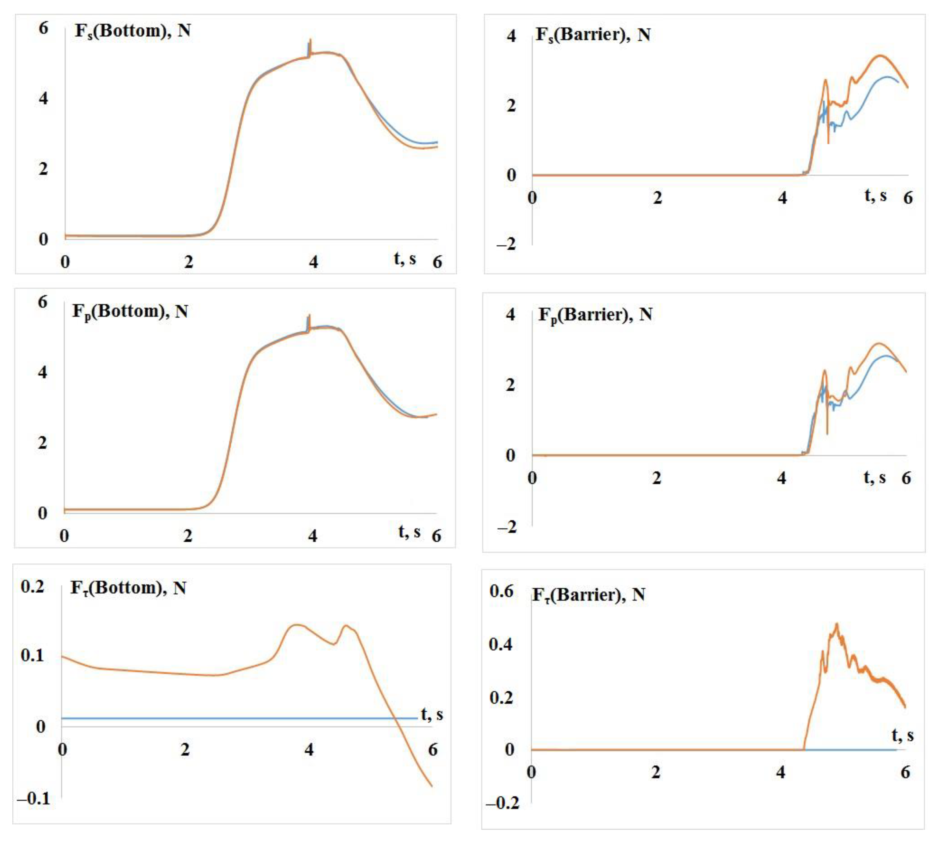
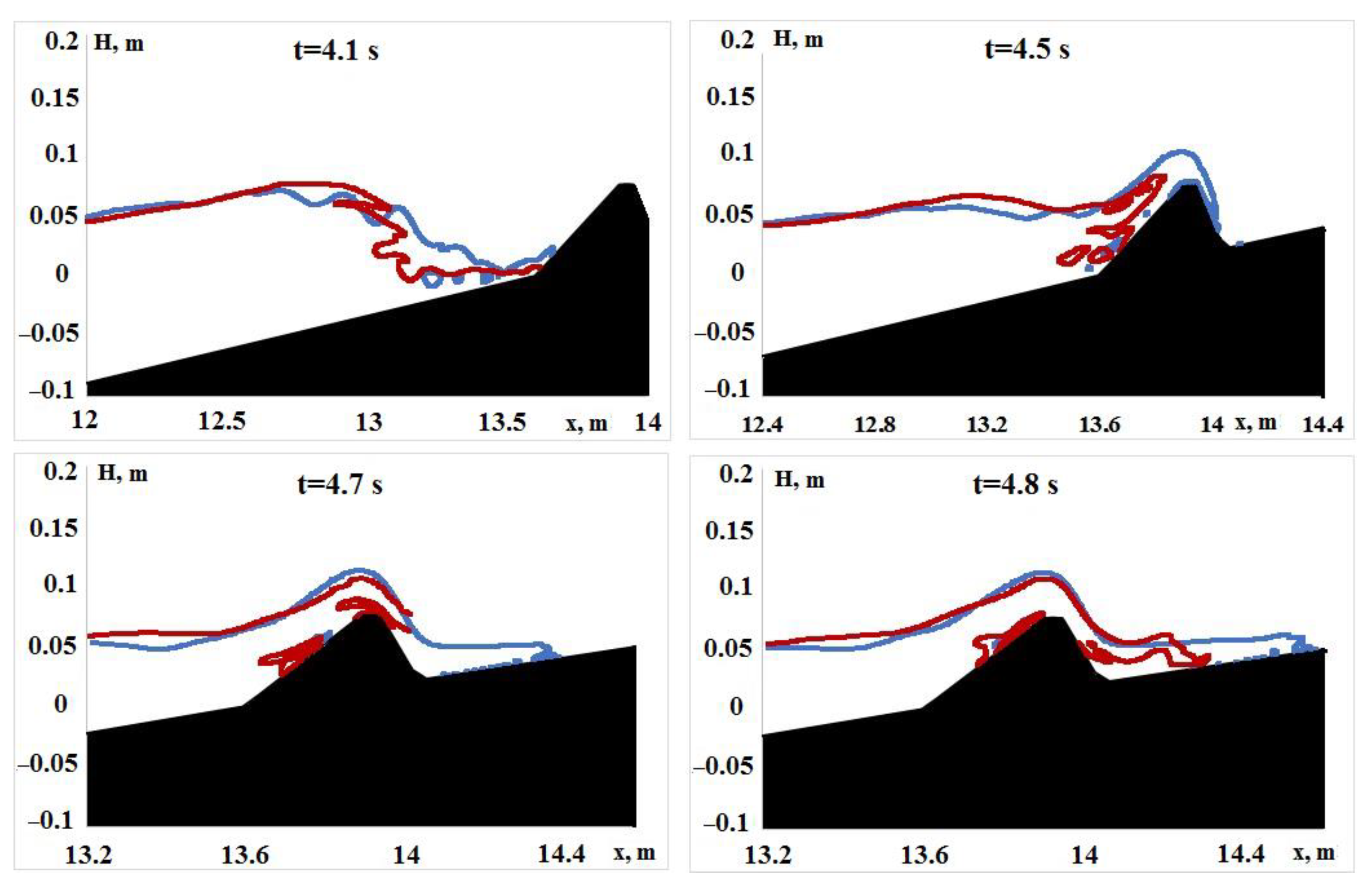
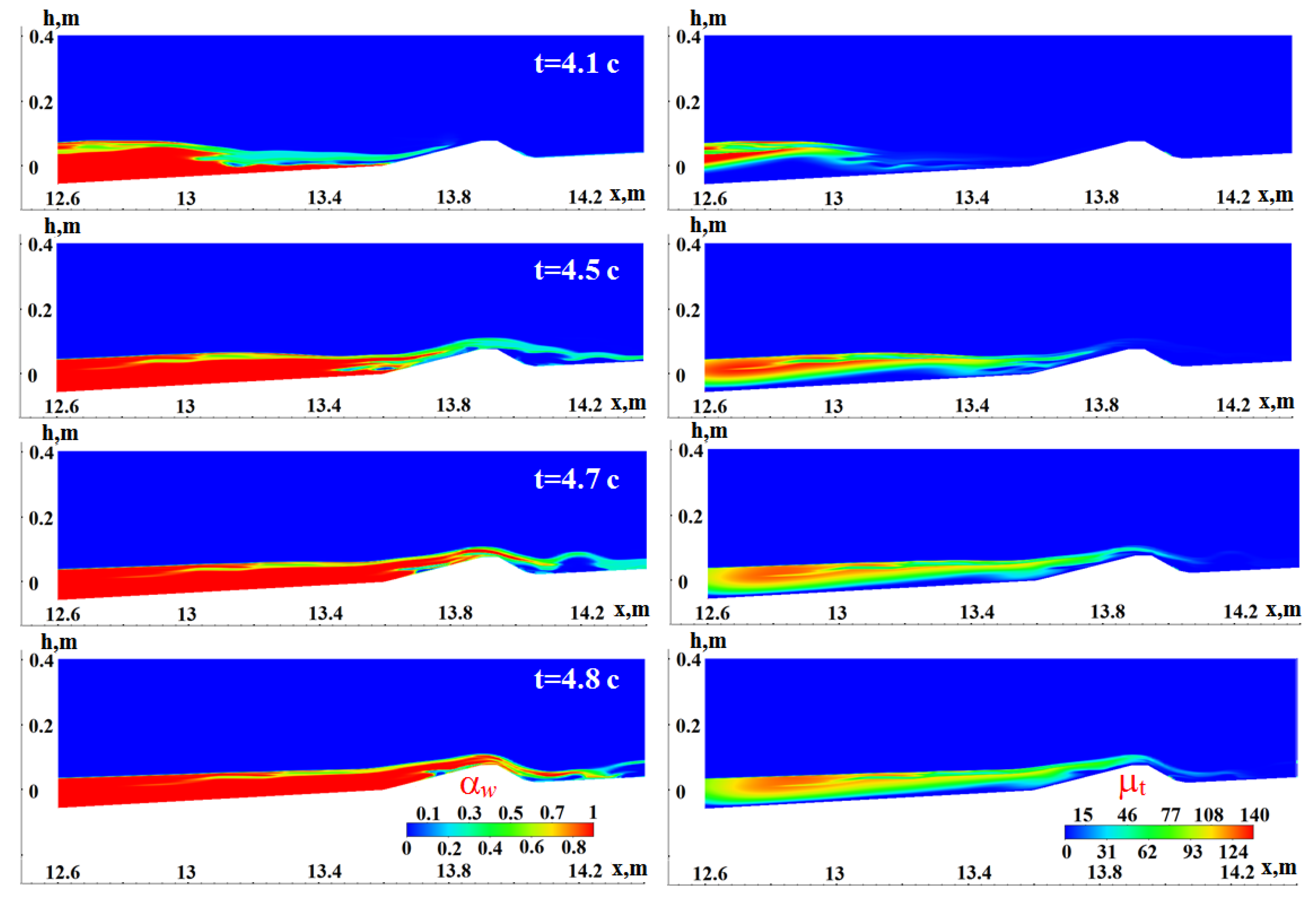
3.2. Setup 2
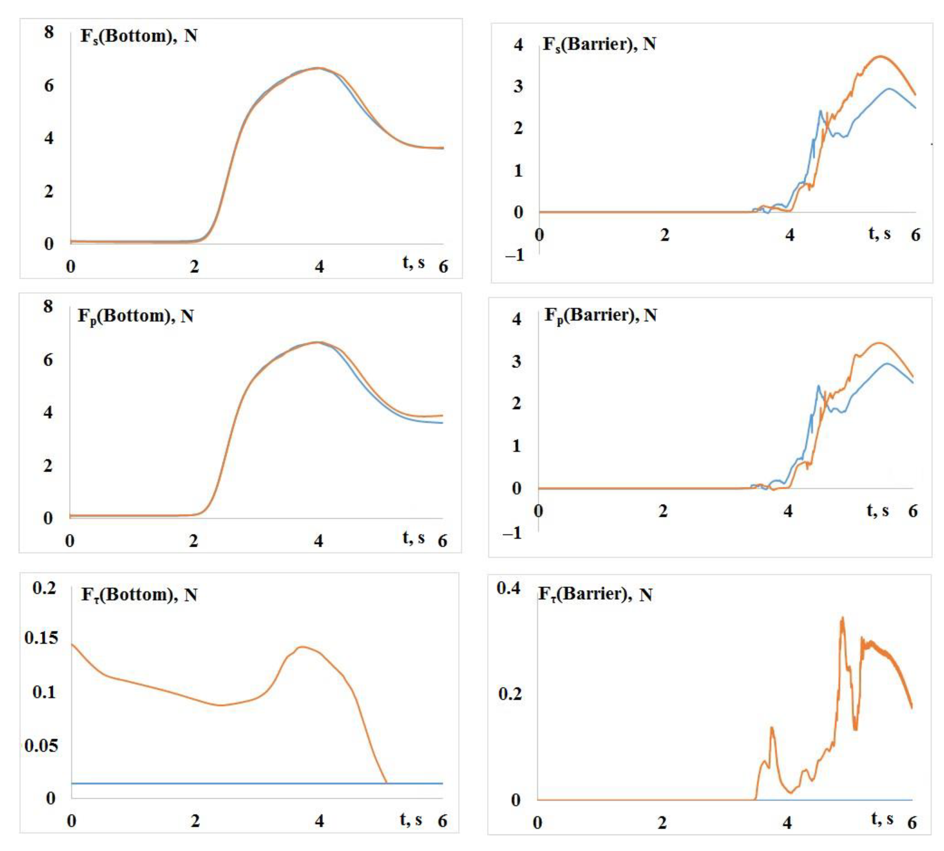
3.3. Setup 3
3.4. Setup 4
4. Conclusions
Author Contributions
Funding
Conflicts of Interest
References
- Landau, L.D.; Lifshitz, E.M. Fluid Mechanics: V. 6; Elsevier: Amsterdam, The Netherlands, 2013; p. 558. [Google Scholar]
- Kim, D.C.; Kim, K.O.; Pelinovsky, E.N.; Didenkulova, I.I.; Choi, B.H. Three-dimensional tsunami runup simulation for the port of Koborinai on the Sanriku coast of Japan. J. Coast. Res. 2013, 65, 266–271. [Google Scholar] [CrossRef]
- Yuk, D.; Yim, S.C.; Liu, P.L.-F. Numerical modeling of submarine mass-movement generated waves using RANS model. Comput. Geosci. 2006, 32, 927–935. [Google Scholar] [CrossRef]
- Zhao, Q.; Armfield, S.; Tanimoto, K. Numerical simulation of breaking waves by a multi-scale turbulence model. Coast. Eng. 2004, 51, 53–80. [Google Scholar] [CrossRef]
- Choi, B.H.; Kim, D.C.; Pelinovsky, E.; Woo, S.B. Three-dimensional simulation of tsunami run-up around conical island. Coast. Eng. 2007, 54, 618–629. [Google Scholar] [CrossRef]
- Pelinovsky, E.; Choi, B.H.; Talipova, T.; Woo, S.B.; Kim, D.C. Solitary wave transformation on the underwater step: Asymptotic theory and numerical experiments. Appl. Math. Comput. 2010, 217, 1704–1718. [Google Scholar] [CrossRef]
- Choi, B.H.; Pelinovsky, E.; Kim, D.C.; Didenkulova, I.; Woo, S.-B. Two- and three-dimensional computation of solitary wave runup on non-plane beach. Nonlinear Processes Geophys. 2008, 15, 489–502. [Google Scholar] [CrossRef]
- Garbaruk, A.V.; Strelets, M.K.; Travin, A.K.; Shur, M.L. Up-to-Date Approaches to Turbulence Simulations: A Study Guide; Publishing House of Peter the Great St./Petersburg Polytechnic University: Saint Petersburg, Russia, 2016; p. 233. [Google Scholar]
- Volkov, K.N.; Emelyanov, V.N. Large Eddy Simulations in Calculations of Turbulent Flows; Fizmatlit: Moscow, Russia, 2008; p. 368. [Google Scholar]
- Belov, I.A.; Isaev, S.A. Simulations of Turbulent Flows: A Study Guide; Publishing House of Baltic State Technical University: Saint Petersburg, Russia, 2001; p. 108. [Google Scholar]
- Lesieur, M. Turbulence in Fluids, 4th ed.; Springer: Dordrecht, The Netherlands, 2008; p. 558. [Google Scholar]
- Tanaka, H.; Tinh, N.X.; Sana, A. Transitional Behavior of a Flow Regime in Shoaling Tsunami Boundary Layers. J. Mar. Sci. Eng. 2020, 8, 700. [Google Scholar] [CrossRef]
- Sana, A.; Tanaka, H. Numerical modeling of a turbulent bottom boundary layer under solitary waves on a smooth surface. Coast. Eng. Proc. 2018, 36, 152266. [Google Scholar] [CrossRef][Green Version]
- Tinh, N.X.; Tanaka, H. Study on boundary layer development and bottom shear stress beneath a tsunami. Coast. Eng. J. 2019, 61, 574–589. [Google Scholar] [CrossRef]
- Sana, A.; Tanaka, H. Two-equation turbulence modeling of an oscillatory boundary layer under steep pressure gradient. Can. J. Civ. Eng. 2010, 37, 648–656. [Google Scholar] [CrossRef]
- Kozelkov, A.S.; Kurulin, V.V.; Tyatyushkina, E.S.; Puchkova, O.L. Application of the detached-eddy simulation model for viscous incompressible turbulent flow simulations on unstructured grids. Math. Models Comput. Simul. 2014, 26, 81–96. [Google Scholar]
- Kozelkov, A.; Kurulin, V.; Emelyanov, V.; Tyatyushkina, E.; Volkov, K. Comparison of convective flux discretization schemes in detached-eddy simulation of turbulent flows on unstructured meshes. J. Sci. Comput. 2016, 67, 176–191. [Google Scholar] [CrossRef]
- Menter, F.R.; Kuntz, M.; Langtry, R. Ten Years of Industrial Experience with the SST Turbulence Model. In Turbulence, Heat and Mass Transfer, 4th ed.; Hanjalic, K., Nagano, Y., Tummers, M., Eds.; Begell House Inc.: Danbury, CT, USA, 2003; pp. 625–632. [Google Scholar]
- Zaikov, L.A.; Strelets, M.K.; Shur, M.L. A comparison between one- and two-equation differential turbulence models in application to separated and attached flows: Flow in channels with counter. High Temp. 1996, 34, 713–725. [Google Scholar]
- Ubbink, O. Numerical Prediction of Two Fluid Systems with Sharp Interfaces. Ph.D. Thesis, Imperial College of Science, Technology & Medicine, London, UK, 1997. [Google Scholar]
- Khrabry, A.I.; Zaytsev, D.K.; Smirnov, E.M. Numerical simulations of free-surface flows based on the VOF method. Trans. Krylov State Res. Cent. 2003, 78, 53–64. [Google Scholar]
- Kozelkov, A.S. The Numerical Technique for the Landslide Tsunami Simulations Based on Navier-Stokes Equations. J. Appl. Mech. Tech. Phys. 2017, 58, 1192–1210. [Google Scholar] [CrossRef]
- Kozelkov, A.S.; Efremov, V.R.; Kurkin, A.A.; Pelinovsky, E.N.; Tarasova, N.V.; Strelets, D.Y. Three dimensional numerical simulation of tsunami waves based on the Navier-Stokes equations. Sci. Tsunami Hazards 2017, 36, 183–196. [Google Scholar]
- Kozelkov, A.S.; Kurulin, V.V.; Lashkin, S.V.; Shagaliev, R.M.; Yalozo, A.V. Investigation of supercomputer capabilities for the scalable numerical simulation of computational fluid dynamics problems in industrial applications. Comput. Math. Math. Phys. 2016, 56, 1506–1516. [Google Scholar] [CrossRef]
- Chen, Z.J.; Przekwas, A.J. A coupled pressure-based computational method for incompressible/compressible flows. J. Comput. Phys. 2010, 229, 9150–9165. [Google Scholar] [CrossRef]
- Kozelkov, A.S.; Lashkin, S.V.; Efremov, V.R.; Volkov, K.N.; Tsibereva, Y.A.; Tarasova, N.V. An implicit algorithm of solving Navier–Stokes equations to simulate flows in anisotropic porous media. Comput. Fluids 2018, 160, 164–174. [Google Scholar] [CrossRef]
- Kozelkov, A.S.; Kurkin, A.A.; Sharipova, I.L.; Kurulin, V.V.; Pelinovsky, E.N.; Tyatyushkina, E.S.; Meleshkina, D.P.; Lashkin, S.V.; Tarasova, N.V. A minimum basic set of validation problems for free-surface flow simulation methods. Trans. NNSTU N.A. R.E. Alekseev. 2015, 2, 49–69. [Google Scholar]
- Tyatyushkina, E.S.; Kozelkov, A.S.; Kurkin, A.A.; Pelinovsky, E.N.; Kurulin, V.V.; Plygunova, К.S.; Utkin, D.A. Verification of the LOGOS Software Package for Tsunami Simulations. Geosciences 2020, 10, 385. [Google Scholar] [CrossRef]
- Kozelkov, A.S.; Kurkin, A.A.; Pelinovsky, E.N.; Kurulin, V.V.; Tyatyushkina, E.S. Modeling the Disturbances in the Lake Chebarkul Caused by the Fall of the Meteorite in 2013. Fluid Dyn. 2015, 50, 828–840. [Google Scholar] [CrossRef]
- Kozelkov, A.S.; Kurkin, A.A.; Pelinovsky, E.N.; Kurulin, V.V. Modeling the cosmogenic tsunami within the framework of the Navier-Stokes equations with sources of different type. Fluid Dyn. 2015, 50, 306–313. [Google Scholar] [CrossRef]
- Hsiao, S.-C.; Lin, T.-C. Tsunami-like solitary waves impinging and overtopping an impermeable seawall: Experiment and RANS modeling. Coast. Eng. 2010, 57, 1–18. [Google Scholar] [CrossRef]


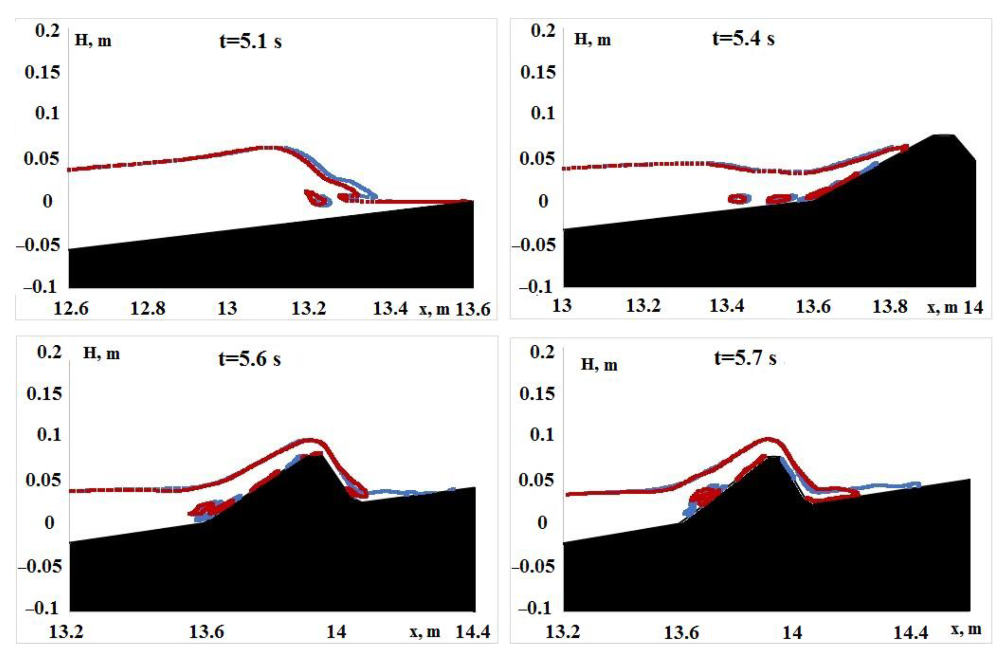
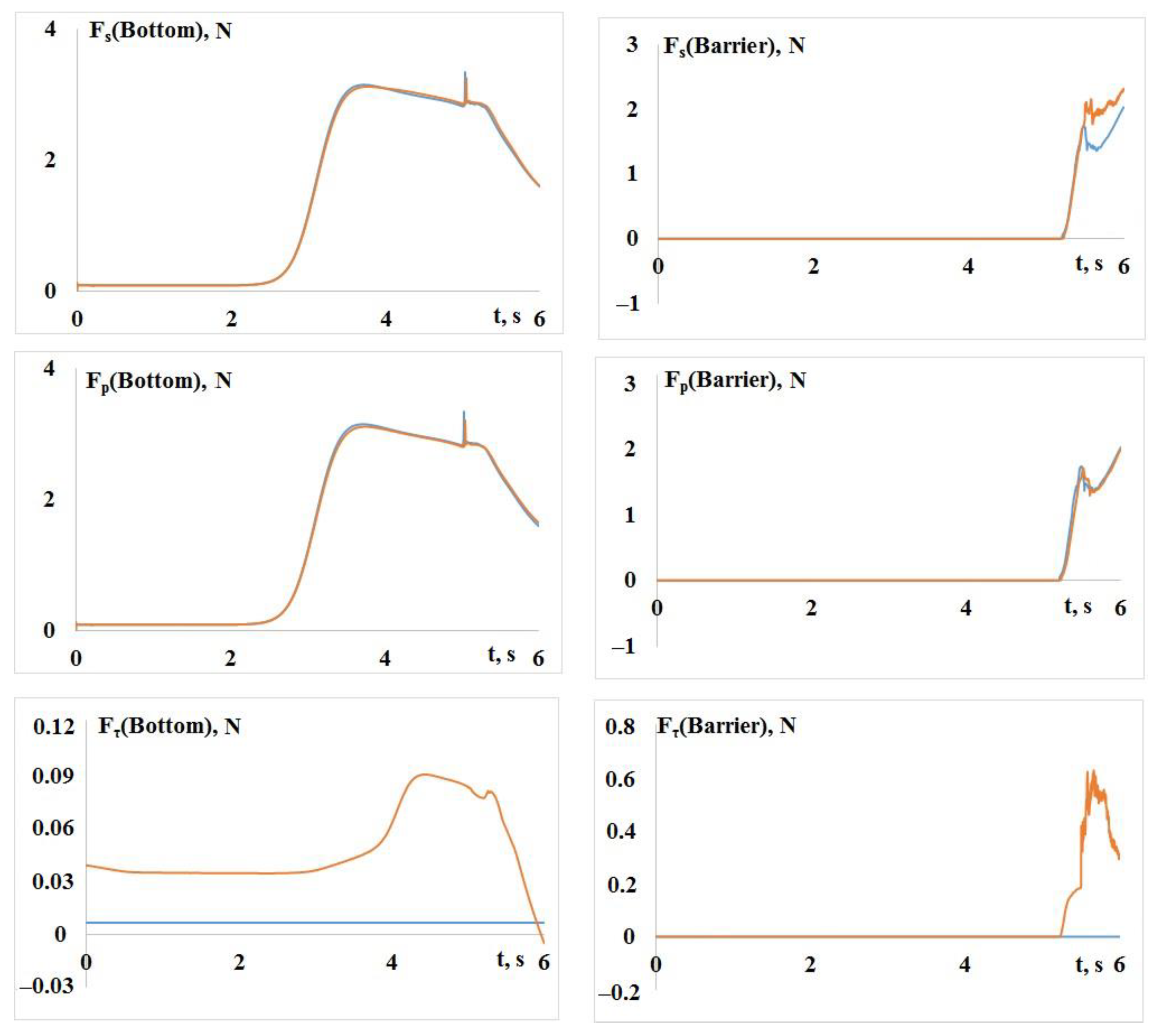
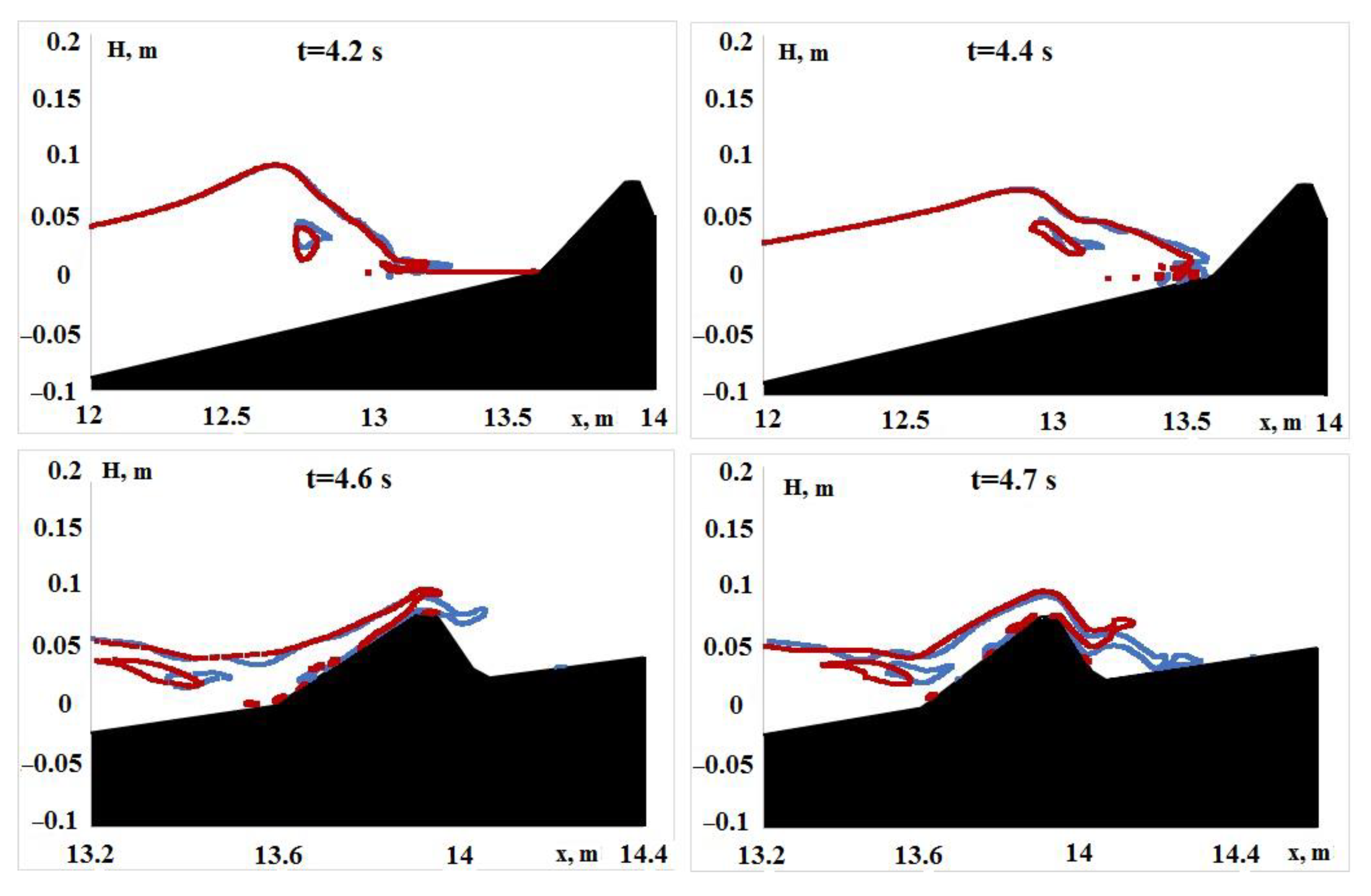
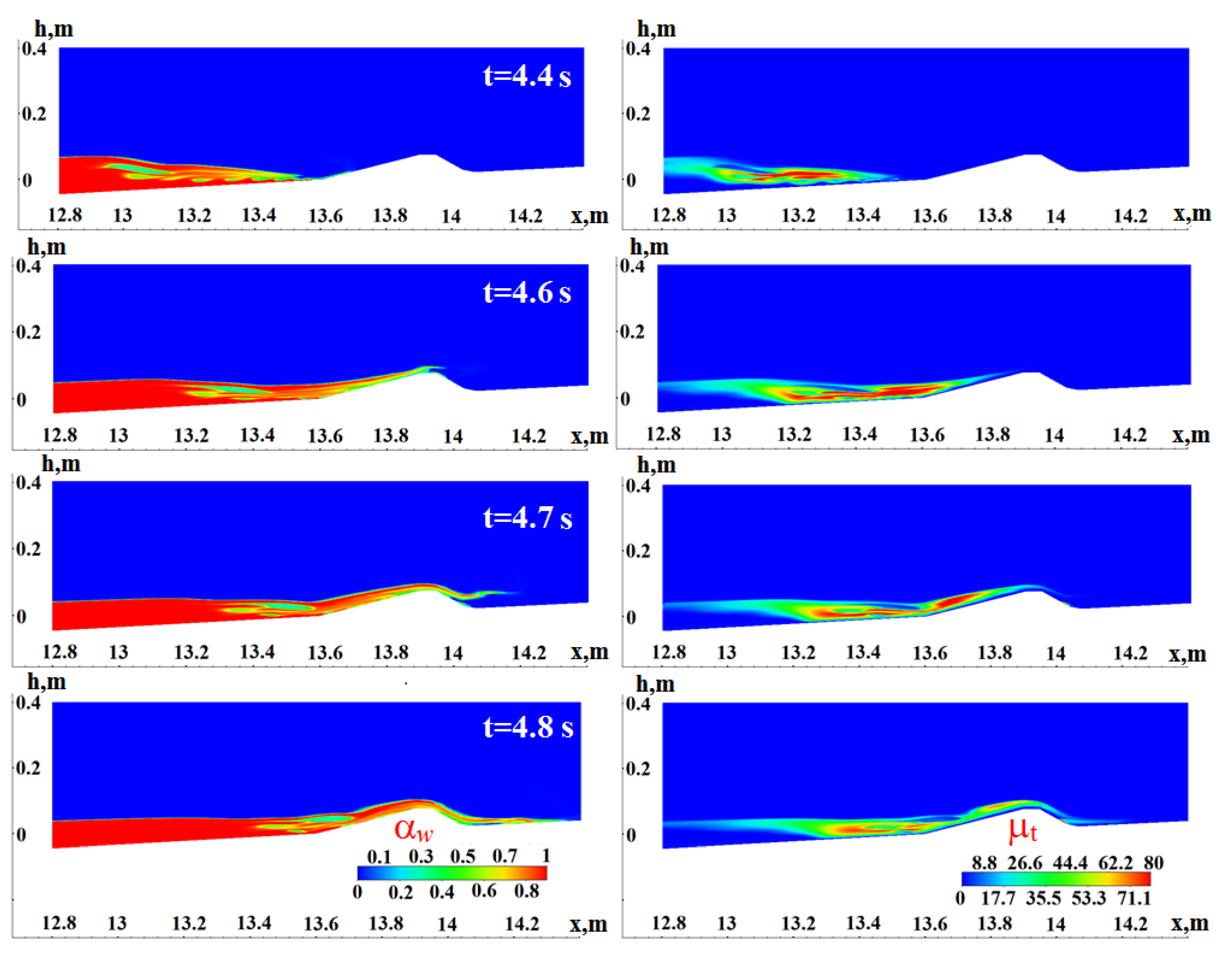
 —without TM,
  —with TM).
 —without TM,
  —with TM).
—without TM, —with TM).
—with TM).
—without TM, —with TM).
 —without TM,
  —with TM).

 —without TM,
  —with TM).
—without TM, —with TM).
—with TM).
—without TM, —with TM).
 —without TM,
  —with TM).

 —without TM,
  —with TM).
—without TM, —with TM).
—with TM).
—without TM, —with TM).
 —without TM,
  —with TM).

 —without TM,
  —with TM).
—without TM, —with TM).
—with TM).
—without TM, —with TM).

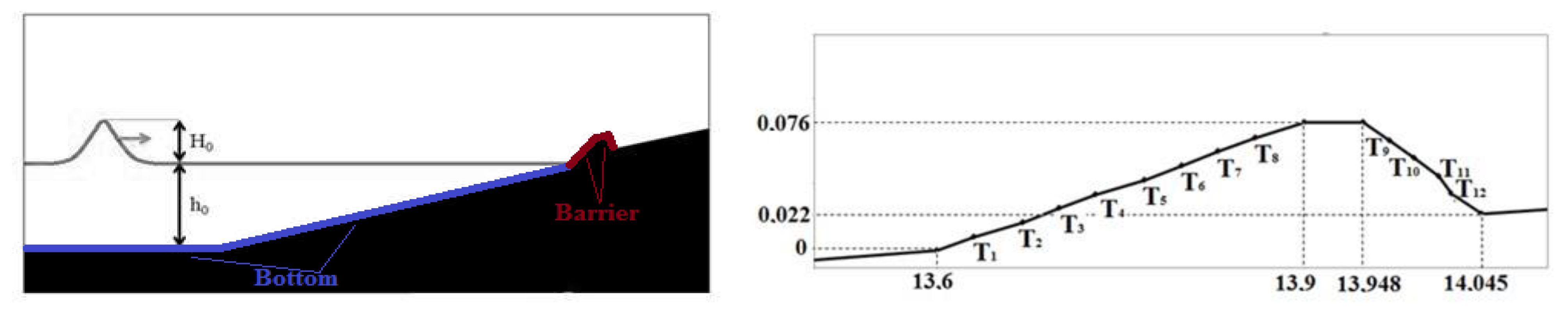
| Point (Figure 1, Right) | Coordinates | Point (Figure 1, Right) | Coordinates | Point (Figure 1, Right) | Coordinates |
|---|---|---|---|---|---|
| T1 | (13.63, 0.008) m | T5 | (13.77, 0.042) m | T9 | (13.97, 0.065) m |
| T2 | (13.67, 0.017) m | T6 | (13.80, 0.050) m | T10 | (13.99, 0.055) m |
| T3 | (13.70, 0.025) m | T7 | (13.83, 0.059) m | T11 | (14.01, 0.044) m |
| T4 | (13.73, 0.033) m | T8 | (13.86, 0.067) m | T12 | (14.02, 0.034) m |
| Setup No.: | Reynolds Number | H0, m |
|---|---|---|
| 1 | 2.8 × 10⁴ | 0.02 |
| 2 | 1.92 × 10⁵ | 0.07 |
| 3 | 5.4 × 10⁵ | 0.12 |
| 4 | 7.2 × 10⁵ | 0.15 |
Publisher’s Note: MDPI stays neutral with regard to jurisdictional claims in published maps and institutional affiliations. |
© 2022 by the authors. Licensee MDPI, Basel, Switzerland. This article is an open access article distributed under the terms and conditions of the Creative Commons Attribution (CC BY) license (https://creativecommons.org/licenses/by/4.0/).
Share and Cite
Kozelkov, A.; Tyatyushkina, E.; Kurulin, V.; Kurkin, A. Influence of Turbulence Effects on the Runup of Tsunami Waves on the Shore within the Framework of the Navier–Stokes Equations. Fluids 2022, 7, 117. https://doi.org/10.3390/fluids7030117
Kozelkov A, Tyatyushkina E, Kurulin V, Kurkin A. Influence of Turbulence Effects on the Runup of Tsunami Waves on the Shore within the Framework of the Navier–Stokes Equations. Fluids. 2022; 7(3):117. https://doi.org/10.3390/fluids7030117
Chicago/Turabian StyleKozelkov, Andrey, Elena Tyatyushkina, Vadim Kurulin, and Andrey Kurkin. 2022. "Influence of Turbulence Effects on the Runup of Tsunami Waves on the Shore within the Framework of the Navier–Stokes Equations" Fluids 7, no. 3: 117. https://doi.org/10.3390/fluids7030117
APA StyleKozelkov, A., Tyatyushkina, E., Kurulin, V., & Kurkin, A. (2022). Influence of Turbulence Effects on the Runup of Tsunami Waves on the Shore within the Framework of the Navier–Stokes Equations. Fluids, 7(3), 117. https://doi.org/10.3390/fluids7030117