Numerical Simulation of Irregular Breaking Waves Using a Coupled Artificial Compressibility Method

Abstract

Wave breaking is widely recognized as a very challenging phenomenon to emulate using numerical/computational methods. On that condition, the transition from modelling regular to irregular breaking waves is not trivial. Even though some issues are surpassed in CFD simulations, there still are two substantial problems to account for. The first one entails the proper generation of irregular waves in a numerical wave tank, while the second is the introduction of the turbulent regime of breaking in the solver. The present work addresses these two problems by employing the Stabilized $k-\omega$ SST model for turbulence closure and by proposing an efficient and accurate method for irregular wave generation. Apart from that, an artificial compressibility method is used for coupling the system of equations, which solves these equations in a non-segregated manner and overcomes problems pertaining to the existence of the interface in free-surface flows. The methodology is validated through the test case of irregular wave propagation over a submerged breaker bar and a piecewise sloped bottom, indicating the ability of the method to capture irregular breaking wave phenomena. Simulations are in fair agreement with experimental data regarding energy spectra and free surface time-series, while results suggest that the known over-prediction of turbulent kinetic energy (TKE) is significantly constrained by the stabilized $k-\omega$ SST model.

1. Introduction

When studying water waves, the consideration of a motion that consists of individual waves of the same frequency and height might provide significant results but is quite idealistic and of limited practical utility. Ocean wave patterns tend to continuously change with time and space in an unrepeatable and non-deterministic manner; therefore, the investigation of real sea states is proven to be highly complex. Considering the complexities, the focus on irregular breaking waves is one of the most challenging tasks. In particular, wave breaking is one of the most interesting phenomena that occurs in shallow waters and also presents very complicated dynamics regarding the fluid’s motion.

Experiments have been widely used for the study of irregular breaking waves; however, during recent years, numerical models of different origins have emerged and gained profound popularity. Reynolds-Averaged Navier–Stokes equations (RANS) constitute a good numerical approach for the modelling of the wave transformation over sloping seabeds [1]. Classical potential flow theory formulations disregard the influence of viscosity and turbulence production, which plays a significant role in the investigation of surf zone dynamics. Thus, they require a coupling with semi-empirical viscosity models [2]. In addition, Computational Fluid Dynamics (CFD) has become widely popular due to its cost-effectiveness and relative accuracy in comparison with experiments, as well as its ability to surpass scale effects.

In RANS simulations of regular breaking waves, the problem of turbulence modelling was addressed and highlighted from the beginning. Especially the difficulty of capturing the adverse transformations of the free-surface upon breaking. In particular, Lin and Liu [1] simulated spilling breakers using a single-phase algebraic $k-ϵ$ turbulence model and the VOF method. One of their major findings was the sensitivity of the simulated wave profile and the respective turbulent kinetic energy for different turbulence closure approaches. Moreover, Bradford [3] used $k-ϵ$ and Re-Normalization Group (RNG) $k-ϵ$ models to simulate spilling and plunging waves and identified the limitations of VOF in capturing the overturning of a plunging breaker, which according to the author’s opinion, might also be due to the nonphysically large dissipation of the turbulence models. Additionally, Mayer and Madsen [4] used an ad hoc modification of the TKE production term for the $k-\omega$ model by using the mean flow vorticity instead of the mean velocity gradient. Under this scope, the overproduction of TKE and the excessive wave damping in the potential flow pre-breaking regions were eliminated, and the agreement with the experimental results was significantly ameliorated. More recently, Chella [5] has implemented the Level Set Method (LSM) with a $k-\omega$ turbulence model to investigate the wave breaking over a seabed. Brown et al. [6] conducted an evaluation of different RANS turbulence closure models and compared their accuracy and efficiency regarding the capturing of wave breaking. They showed that the most suitable are the nonlinear $k-ϵ$, the $k-\omega$ SST and the Reynolds Stress Model. Furthermore, Devolder et al. [7] identified the issue of the inherent damping of non-breaking waves in the vicinity of the free-surface and developed a Buoyancy Modified $k-\omega$ and $k-\omega$ SST model to address this issue. The essence of this approach is the transition to a laminar regime in the region where the wave propagates without deforming and the recovery of the turbulence model in the surf zone, where large horizontal density gradients are present. Although results showed an improved agreement with experiments, the author highlighted that the problem of turbulent kinetic energy over-prediction remains unresolved. Larsen and Fuhrman [8] showed that all the turbulence models in the literature were subject to irrepressible growth of the turbulent kinetic energy, as well as the eddy viscosity, and thus were unconditionally unstable. For this reason, they introduced the Stabilized $k-\omega$ SST model, which further limits the eddy viscosity in regions where the flow is nearly potential. Liu et al. [9] have implemented the modified VOF method with free-surface jump conditions to study wave breaking in order to address the issue of spurious air velocities described by Vukcevic et al. [10].

Regarding the generation of irregular waves in CFD-based numerical wave tanks, Lara et al. [11] have presented the application of a method for generating irregular waves through the use of internal wavemakers with a mass-source function. This approach, first introduced by Lin and Liu [12] proved to be quite precise for the generation of irregular patterns from a given spectrum. More recently, Paulsen et al. [13] carried out numerical simulations in order to study the irregular wave loads on monopiles. Gatin et al. [14] developed a framework for simulation of irregular waves using a RANS model coupled with a Higher-Order Spectral (HOS) method, which led to increased computational efficiency.

Even though both of the aforementioned topics have been addressed individually, the literature pertaining to irregular breaking waves that combines these two areas is rather limited. Aggarwal et al. [15] have developed a method for the numerical simulation of irregular waves and used it for the investigation of breaking wave properties [16] and the breaking-wave–structure interaction [17]. However, throughout the described work, the influence of turbulence is not the prime concern and the standard $k-\omega$ model is used, despite its known shortcomings. In the present work, an investigation of irregular breaking waves is made using the stabilized $k-\omega$ SST model. Initially, the wave generation, the method described in [12] for producing irregular waves from a given spectrum is slightly modified to fit the in-house solver MaPFlow. Afterward, the capacity of the solver in the simple propagation of irregular waves is studied, and then two test cases of propagation over a submerged bar and a piecewise sloped seabed are considered, where computational results are compared with available experimental data.

2. Governing Equations

Considering an incompressible fluid medium, the equations of the conservation of mass and momentum, respectively, will be

$$\nabla \overrightarrow{u}=0$$

(1)

$$\frac{\partial \overrightarrow{u}}{\partial t}+\overrightarrow{u}\nabla \overrightarrow{u}=-\frac{1}{\rho }\nabla p+\nabla \overline{\sigma }+{\overrightarrow{F}}_B$$

(2)

where $\rho$ denotes the fluid density, $\overrightarrow{u}$ the velocity vector, p the pressure, ${\overrightarrow{F}}_B$ the source terms and body forces’ density and $\overline{\sigma }$ the stress tensor.

For the simulation of two-phase flows, the Volume-Of-Fluid (VOF) method [18] is used, which translates the presence of the liquid or the gas phase in a certain region to the value of the volume fraction

$${\alpha }_l=\frac{{\rho }_m-{\rho }_a}{{\rho }_w-{\rho }_a}$$

(3)

where the index w corresponds to the liquid phase and a to the gas phase. It is evident that the volume fraction takes the values 1 and 0 for water and air, respectively, while at the interface of the fluids, it takes an interim value. In this area, which defines the vicinity of the free surface, the properties of the mixture fluid are redefined according to the volume fraction and follow

$${\rho }_m=\alpha {\rho }_w+(1-\alpha ){\rho }_a$$

(4)

$${\mu }_m=\alpha {\mu }_w+(1-\alpha ){\mu }_a$$

(5)

Moreover, the free surface is treated as a material surface, hence

$$\frac{D\alpha }{Dt}=\frac{\partial \alpha }{\partial t}+\overrightarrow{u}·\nabla \alpha =0$$

(6)

The artificial compressibility method, proposed by Chorin [19], is implemented in the present study in order to couple the equations of mass and momentum, through the addition of a fictitious time ($\tau$) derivative of pressure

$$\frac{1}{\beta }\frac{\partial p}{\partial \tau }+\rho \nabla \overrightarrow{u}=0$$

(7)

where $\beta$ is the artificial compressibility factor and regulates the influence of the pseudo-time derivative. In fact, it is a free numerical parameter, which corresponds to a pseudo-sound speed, similar to the sound of speed in compressible flows.

$$\frac{\partial p}{\partial \rho }=c^2\Rightarrow \frac{\partial \rho }{\partial p}{|}_{\tau }=\frac{1}{\beta }$$

(8)

The system that is constituted by Equations (1), (2) and (6) can fully describe viscous two-phase flows.

$$\Gamma {\int }_{\Omega }\frac{\partial \overrightarrow{Q}}{\partial \tau }d\Omega +{\Gamma }_e{\int }_{\Omega }\frac{\partial \overrightarrow{Q}}{\partial t}d\Omega =-{\oint }_{\partial \Omega }({\overrightarrow{F}}_c-{\overrightarrow{F}}_v)dS+{\int }_{\Omega }{\overrightarrow{S}}_{q}d\Omega$$

(9)

where $\Gamma$ is the preconditioner of Kunz [20], used in order to counteract the problem of stiff matrices that occur when high-density ratios appear in the eigenvalues of the system. Vector $\overrightarrow{Q}$ is the matrix of primitive variables, whereas $\overrightarrow{U}$ are the respective conservative variables. It is worth noticing that the unsteady system of equations is expressed for the conservative variables $\overrightarrow{U}$ at each physical timestep, but at each fictitious timestep, a pseudo-steady state problem is solved for the primitive equations $\overrightarrow{Q}$. The transformation from the latter to the former is achieved through the Jacobian matrix ${\Gamma }_e=\frac{\partial \overrightarrow{U}}{\partial \overrightarrow{Q}}$.

$$\overrightarrow{U}={\left[\begin{array}{ccc}0& \rho \overrightarrow{u}& {\alpha }_l\end{array}\right]}^T\overrightarrow{Q}={\left[\begin{array}{ccc}p& \overrightarrow{u}& {\alpha }_l\end{array}\right]}^T$$

(10)

$$\Gamma =\left[\begin{array}{ccc}\frac{1}{\beta {\rho }_m}& 0& 0\\ 0& {\rho }_{m}I& \overrightarrow{u}\Delta \rho \\ \frac{{\alpha }_l}{\beta {\rho }_m}& 0& 1\end{array}\right]{\Gamma }_e=\left[\begin{array}{ccc}0& 0& 0\\ 0& {\rho }_{m}I& \overrightarrow{u}\Delta \rho \\ 0& 0& 1\end{array}\right]$$

(11)

Moreover, ${\overrightarrow{F}}_c$ and ${\overrightarrow{F}}_v$ denote the inviscid and viscous fluxes, respectively, described as

$${\overrightarrow{F}}_c=\left[\begin{array}{c}{V}_n\\ {\rho }_{m}u{V}_n+p{n}_x\\ {\rho }_{m}v{V}_n+p{n}_y\\ {\rho }_{m}w{V}_n+p{n}_z\\ {\alpha }_l{V}_n\end{array}\right]{\overrightarrow{F}}_v=\left[\begin{array}{c}0\\ {\tau }_{xx}{n}_x+{\tau }_{xy}{n}_y+{\tau }_{xz}{n}_z\\ {\tau }_{yx}{n}_x+{\tau }_{yy}{n}_y+{\tau }_{yz}{n}_z\\ {\tau }_{zx}{n}_x+{\tau }_{zy}{n}_y+{\tau }_{zz}{n}_z\\ 0\end{array}\right]$$

(12)

where $V_n=\overrightarrow{u}·\overrightarrow{n}$. The velocity ${\overrightarrow{u}}_{vol}$ corresponds to the movement of the control volume and $\overrightarrow{n}$ denotes the surface normal of the control volume.

The viscous stresses ${\tau }_{ij}$, according to Boussinesq’ hypothesis follow,

$${\tau }_{ij}=({\mu }_m+{\mu }_t)(\frac{\partial u_i}{\partial x_j}+\frac{\partial u_j}{\partial x_i})-\frac{2}{3}\rho {\delta }_{ij}k$$

(13)

where ${\mu }_t$ is the turbulent dynamic viscosity, k is the turbulent kinetic energy and ${\delta }_{ij}$ is the Kronecker delta.

3. Numerical Method

3.1. Spatial Discretization

The primitive variables for a control volume ${\Omega }_i$ will be integrated to

$$\overrightarrow{\overline{Q}}=\frac{1}{{\Omega }_i}{\int }_{{\Omega }_i}\overrightarrow{Q}(\overrightarrow{x};t)d\Omega$$

(14)

By gathering the right-hand side terms of Equation (9) in a residual and following the formulation above considering finite volumes, it will follow that

$${\Gamma }_e\frac{\partial (\overrightarrow{\overline{Q}}\Omega )}{\partial t}+\Gamma \frac{\partial (\overrightarrow{\overline{Q}}\Omega )}{\partial \tau }=-{\overrightarrow{R}}_{\Omega }$$

(15)

where

$${\overrightarrow{R}}_{\Omega }={\oint }_{\partial {\Omega }_i(t)}({\overrightarrow{F}}_c-{\overrightarrow{F}}_v)dS-{\int }_{{\Omega }_i(t)}{\overrightarrow{S}}_{q}d\Omega$$

(16)

Assuming that the surface integral of the residual ${\overrightarrow{R}}_{\Omega }$ does not vary across different edges of each cell, it can be approximated as a sum of the fluxes evaluated at each face midpoint. In addition, the volume integral of the source term is assumed to be constant throughout each elemental volume. Thus, if $N_f$ is the total number of faces of the corresponding control volume, it can be expressed as

$${\overrightarrow{R}}_{{\Omega }_i}=\sum _j^{N_f}({\overrightarrow{F}}_c-{\overrightarrow{F}}_v)d{S}_i-{\overrightarrow{\overline{S}}}_q{\Omega }_i$$

(17)

As can be noticed in Equation (17), the values of the inviscid fluxes on the cells’ faces are required to proceed. This can be achieved via the extrapolation of the field variables’ values from the center of the cells to the corresponding face. Between two adjacent cells, the common edge will have a left and right state, according to the normal vector on the face, which points from the former to the latter. For the aforementioned process, several reconstruction schemes are employed, which differ based on the nature of each equation. Regarding the velocity field, which is continuous everywhere, the Piecewise Linear Reconstruction can be implemented, as well as for the pressure in one-phase flows.

In two-phase cases, both the pressure gradient and the volume fraction present a strong discontinuity in the vicinity of the free surface due to the density jump, and this transitional area must be taken into account appropriately. Regarding the pressure field, a condition of $\left[\frac{\nabla p}{\rho }\right]=0$ is required, which is treated by the density-based interpolation scheme of Qeuetey et al. [21] near the free surface. Proceeding with $\alpha$, which is discontinuous by its definition, special treatment should also be given in order to preserve the associated interface sharpness and hinder excessive smearing due to numerical diffusion. For this purpose, the PLR scheme is used for the volume fraction away from the free surface, while at this region, an interface capturing scheme is activated, which was selected to be HRIC [22] for the present study.

On each cell face, two different values ${\overrightarrow{Q}}_R$ and ${\overrightarrow{Q}}_L$ are extrapolated, and a local Riemann problem is solved between the left and the right state. In this work, the approximate Riemann solver of Roe [23] is used in combination with the preconditioning matrix $\Gamma$ to scale the eigenvalues of the system. A more extensive description of the convective and viscous fluxes’ calculation, as well as of the variable reconstruction process, can be found in [24].

3.2. Temporal Discretization

Proceeding with the discretization of the governing equations in the time scale, considering ${\overrightarrow{Q}}^{*}$ as the flow variables, the constituted implicit formulation will be

$$\Gamma \frac{\partial ({\overrightarrow{Q}}^{*}\Omega )}{\partial \tau }+{\overrightarrow{R}}^{*}=0$$

(18)

where ${\overrightarrow{R}}^{*}$ is the unsteady residual, including the spatial residual (16), as well as the unsteady term as per below

$${\overrightarrow{R}}^{*}={\overrightarrow{R}}_{\Omega }({\overrightarrow{Q}}^{*})+{\Gamma }_e\frac{\partial ({\overrightarrow{Q}}^{*}\Omega )}{\partial t}$$

(19)

Under the scope of dual time-stepping, two indices n and k are introduced to describe the iterations for the physical time and the fictitious time (or internal), respectively. In particular, for every computational step, a pseudo-steady problem is solved, starting with $k=0$, and the flow variables vector is initialized based on the previous convergent solution so that ${\overrightarrow{Q}}_0^{*,n+1}={\overrightarrow{Q}}_k^n$. During this process, ${\overrightarrow{Q}}^{*}$ does not satisfy the original equation, whereas upon convergence, the term $\Gamma \frac{\partial ({\overrightarrow{Q}}^{*}\Omega )}{\partial \tau }$ is eliminated, and the initial equations are recovered.

A Backward Differentiation Formula (BDF) scheme [25] is employed for the discretization of the unsteady term, providing the following series of successive time levels

$$\frac{\partial (\overrightarrow{Q}{\Omega }_i)}{\partial t}=\frac{1}{\Delta t}\left[{\varphi }_{n+1}{({\Omega }_i\overrightarrow{Q})}^{n+1}+{\varphi }_n{({\Omega }_i\overrightarrow{Q})}^n+{\varphi }_{n-1}{({\Omega }_i\overrightarrow{Q})}^{n-1}+\dots \right]$$

(20)

In the present study, two successive time levels were retained, resulting in a second-order accurate discretization. The pseudo-time derivative is discretized using a first-order backward difference scheme as per below

$$\frac{\partial ({\overrightarrow{Q}}^{*}\Omega )}{\partial \tau }={\Omega }_i^{n+1}\frac{{\overrightarrow{Q}}^{*,k+1}-{\overrightarrow{Q}}^{*,k}}{\Delta \tau }$$

(21)

Finally, the local time stepping technique is used for convergence facilitation purposes, according to which the local/cell-specific fictitious timestep is

$$\Delta {\tau }_i=CFL\frac{{\Omega }_i}{{\widehat{\Lambda }}_{c,i}}$$

(22)

where ${\widehat{\Lambda }}_{c,i}$ denotes the convective spectral radii defined as

$${\widehat{\Lambda }}_{c,i}=\sum _{j=1}^{N_f}{\left(|V_n-\frac{V_g}{2}|+c\right)}_{ij}\Delta S_{ij}$$

(23)

3.3. Turbulence Modelling

In the present study, the Stabilized $k-\omega$ SST has been employed, including also the buoyancy term introduced by Devolder et al. [7]. This turbulence closure model was developed by Larsen and Fuhrman [8], who identified all the past turbulence models to be unconditionally unstable in regions of nearly potential flow with finite strain. This argument was backed up by an extension of the analysis of Mayer and Madsen [4], which proved an asymptotic exponential rate of increase in turbulence production in the aforementioned regions, where the mean rotation rate tensor ${\Omega }_{ij}=\frac{1}{2}\left(\frac{\partial u_i}{\partial x_j}-\frac{\partial u_j}{\partial x_i}\right)$ takes near zero values. Hence, according to them, the root cause of the irrepressible growth of the turbulent kinetic energy and the eddy viscosity in surface non-breaking waves is the instability of the standard models in the bulk region below their free surface.

The stabilized $k-\omega$ SST is established on the same advection-diffusion equations for the turbulent kinetic energy k and the specific dissipation rate $\omega$ as introduced by Menter [26] for the original $k-\omega$ SST model

$$\begin{array}{c}\hfill \frac{\partial (\rho k)}{\partial t}+\nabla (\overrightarrow{u}\rho k)=\nabla \left[(\mu +{\sigma }_k{\mu }_t)\nabla k\right]+\rho P_k+G_b-{\beta }^{*}\rho \omega k\\ \hfill \frac{\partial (\rho \omega )}{\partial t}+\nabla (\overrightarrow{u}\rho \omega )=\nabla \left[(\mu +{\sigma }_{\omega }{\mu }_t)\nabla \omega \right]+\alpha \rho S^2-\beta \rho {\omega }^2+2(1-F_1)\frac{\rho {\sigma }_{\omega 2}}{\omega }\nabla k·{(\nabla \omega )}^T\end{array}$$

(24)

where $P_k=\min ({\mu }_t(\nabla \times \overrightarrow{u}){(\nabla \times \overrightarrow{u})}^T,10{\beta }^{*}\rho k\omega )$ is the production term of turbulent kinetic energy, ${\mu }_t$ is the turbulent dynamic viscosity (or eddy viscosity) and $S=\sqrt{2S_{ij}{S}_{ij}}$ is the mean strain rate. Moreover, $F_1$ and $F_2$ are switching functions between the $k-\omega$ and the $k-ϵ$ turbulence models and for $F_1=1$ the equations of the former are solved, while the latter is activated when $F_1=0$. These functions are defined as

$$F_1=tanh\left\{{\left\{\min \left[\max \left(\frac{\sqrt{k}}{{\beta }^{*}\omega y},\frac{500v}{y^2\omega }\right),\frac{4\rho {\sigma }_{\omega 2}k}{C{D}_{k\omega }{y}^2}\right]\right\}}^4\right\}$$

(25)

$$F_2=tanh\{\left[\max {\left(\frac{2\sqrt{k}}{{\beta }^{*}\omega y},\frac{500v}{y^2\omega }\right]}^2\right\}$$

(26)

$$C{D}_{k\omega }=\max \left(2\frac{\rho {\sigma }_{\omega 2}}{\omega }\nabla k·{(\nabla \omega )}^T,{10}^{-10}\right)$$

(27)

The constants for this model are: ${\beta }^{*}=0.09$, ${\alpha }_1=5/9$, ${\beta }_1=0.075$, ${\sigma }_{k1}=0.85$, ${\sigma }_{\omega 1}=0.5$, ${\alpha }_2=0.44$, ${\beta }_2=0.0828$, ${\sigma }_{k2}=1.0$ and ${\sigma }_{\omega 2}=0.856$. These parameters are also subject to blending as per below

$$\varphi =F_1{\varphi }_1+(1-F_1){\varphi }_2$$

(28)

The buoyancy term $G_b$ (Equation (29)), introduced by Devolder et al. [7], is deliberately designed to serve a twofold purpose and is tailor-made for the study of wave shoaling and breaking. In particular, it suppresses the level of turbulence by setting a laminar regime in the zone where the interface is horizontal, and the density gradient is very large, driving ${\mu }_t$ to zero. Apart from that, when the wavefront becomes vertical and the wave breaking occurs, $G_b$ is deactivated, providing a fully turbulent solution of the flow field.

$$G_b=-\frac{{\nu }_t}{0.85}\frac{\partial \rho }{\partial x_i}{g}_i$$

(29)

Finally, a limiter is also imposed on the eddy viscosity of the original $k-\omega$ SST model [26] providing

$${\mu }_t=\frac{\rho {\alpha }_{1}k}{\max \left({\alpha }_1\omega ,S{F}_2,{\alpha }_1{\lambda }_2\frac{\beta }{{\beta }^{*}\alpha }\frac{P_0}{P_{\Omega }}\omega \right)}$$

(30)

where $P_0=2S_{ij}{S}_{ij}$, $P_{\Omega }=2{\Omega }_{ij}{\Omega }_{ij}$, and ${\lambda }_2$ is a constant that denotes the upper limit for the model to be formally stable, considering that $P_{\Omega }/P_0\le {\lambda }_2$. It is worth noticing that the new term will only be activated when the flow is nearly potential due to its insignificant rotation, while the initial Buoyancy Modified $k-\omega$ SST model will be recovered in shear regions.

4. Irregular Wave Generation

4.1. Numerical Wave Tank

Due to the high necessity for efficient and accurate wave generation, several approaches have been developed in recent years, which are termed numerical wave-makers. Some of these methods are: Relaxation Zone Method [27], Static and Dynamic Boundaries [28], Mass Source Method [12] and Impulse Source Method [29]. The same practices, along with the Numerical Beach [30] and the Cell Stretching Method [31], can also be implemented for the artificial damping of the waves. More details, as well as a general overview and assessment of the aforementioned methods for wave generation and absorption, can be found in [32,33].

In the present work, a modified Relaxation Zone Method [27] has been adopted for both wave generation and absorption, termed as the Forcing Zone Method [34]. In particular, the numerical solution inside the generation zone is forced to implicitly converge to a wave profile outlined by a suitable wave theory, while in the damping zone, it is artificially damped in the same way. Absorption of the propagating waves is also required in order to prevent any physical disturbance from reaching the outlet boundary. Both of these procedures are achieved by adding an appropriate source term to the spatial residual of Equation (16), the general form of which is

$${\overrightarrow{S}}_{nwt}=C_{nwt}{\rho }_m(\overrightarrow{\varphi }-{\overrightarrow{\varphi }}_{tar})$$

(31)

In the above equation, the term $\overrightarrow{\varphi }$ stands for variables such as the velocity vector $\overrightarrow{u}$ or the volume fraction a, whereas ${\overrightarrow{\varphi }}_{tar}$ is the value towards which $\overrightarrow{\varphi }$ is driven. The choice of the variables that are included is case-dependent and is correlated with the geometry and the physics of the computational domain. Moreover, the effect of the source term is controlled by the term $C_{nwt}$, which requires special treatment and is provided by the following equation

$$C_{nwt}=\alpha \frac{e^{x_r^n}-1}{e-1}{x}_r=\frac{x_s-x}{x_s-x_e}$$

(32)

where $x_r$ is a non-dimensional normalized space variable and ranges between the starting and ending position of the forcing zone. The parameter $\alpha$ regulates the maximum value of the forcing function, while the parameter n regulates its spatial distribution. The values of these two constants should be selected properly, and a case-specific study is generally suggested, as large values of $\alpha$ may lead to numerical instabilities and hinder convergence, whereas small values of it may not be sufficient for driving the solution to the desired form. The function takes its maximum values in the internal boundaries of the computational domain with the zones and reaches zero at the other end of each zone.

4.2. Irregular Wave Generation Framework

In the case of regular wave propagation, MaPFlow determines the velocity, pressure and free-surface elevation fields in the generation zone through the Linear Wave Theory or the Stream Function Theory, as described by Fenton [35]. However, in the case of irregular waves, the generation is not so straightforward and requires the introduction of the energy density spectrum, which in a discretized form can be written as

$$S_i(\omega )\Delta \omega =\frac{1}{2}{A}_i^2$$

(33)

The general principle of the irregular wave generation in MaPFlow is the implementation of a reverse spectral analysis process and the construction of the corresponding time histories by adding a large number of wave components. For the representation of these components, their linear form is considered, meaning that the free surface elevation is a linear superposition of the regular wave components such that

$$\eta (x,t)=\sum _{i=1}^N{A}_{i}cos(k_{i}x-{\omega }_{i}t+{ϵ}_i)$$

(34)

where index i denotes each wave component in a way that its frequency ${\omega }_i$ is the i-th frequency of the discretized energy spectrum. Its wavenumber $k_i=\frac{2\pi }{{\lambda }_i}$ is determined by solving the dispersion equation, whereas its amplitude, according to the definition of the energy spectrum, follows

$$A_i=\sqrt{2S_i(\omega )\Delta \omega }$$

(35)

where the term $S_i$ denotes the spectral density of the wave component and corresponds to the i-th component of the discretized spectrum, similarly with the frequency. It is important to consider that two generated irregular wave patterns, derived from the same spectrum, that have a different distribution of phase angles will have a different free-surface elevation field but will contain the same amount of energy.

Thus, the horizontal and vertical velocity will be, respectively,

$$u(x,z,t)=\sum _{i=1}^N{A}_i{\omega }_i\frac{cosh\left[k_i(z+h)\right]}{sinh(k_{i}h)}cos(k_{i}x-{\omega }_{i}t+{ϵ}_i)$$

(36)

$$w(x,z,t)=\sum _{i=1}^N{A}_i{\omega }_i\frac{sinh\left[k_i(z+h)\right]}{sinh(k_{i}h)}sin(k_{i}x-{\omega }_{i}t+{ϵ}_i)$$

(37)

Furthermore, the corresponding pressure field will follow

$$p(x,z,t)=\sum _{i=1}^N\rho g{A}_i\frac{cosh\left[k_i(z+h)\right]}{cosh(k_{i}h)}cos(k_{i}x-{\omega }_{i}t+{ϵ}_i)$$

(38)

Therefore, the forcing zone term that is added to the momentum equation can be slightly modified so that it incorporates the sum of the corresponding quantity over all the wave components.

$${\overrightarrow{S}}_{nwt}=C_{nwt}{\rho }_m(\overrightarrow{\varphi }-\sum _{n=1}^N{\overrightarrow{\varphi }}_{tar,i})$$

(39)

4.3. Model Validation

In this section, the framework for the generation of irregular waves described above is validated through the generation and propagation of waves derived from a JONSWAP-type [36] spectrum over a flat bed. The spectrum that was used for the generation of the waves is

$$S(\omega )=\frac{5}{16}{H}_s^2{\omega }_p^4{\omega }^{-5}{e}^{-\frac{5}{4}{(\frac{\omega }{{\omega }_p})}^{-4}}{\gamma }^{e^{\frac{-{(\omega -{\omega }_p)}^2}{2{\sigma }^2{\omega }_p^2}}}{A}_{\gamma }$$

(40)

where $\omega$ is the angular frequency over which the spectral density $S(\omega )$ is distributed, $H_s$ is the significant wave height, ${\omega }_p=\frac{2\pi }{T}$ is the peak angular frequency, $\gamma =3.3$ is the peak enhancement factor, $A_{\gamma }=1-0.287\ln \gamma$ and $\sigma =0.07$ for $\omega <{\omega }_p$ or $\sigma =0.09$ for $\omega >{\omega }_p$.

Under that scope, the numerical wave tank shown in Figure 1 was constructed, and a spectrum of peak period $T_p=2$ s and significant height $H_s=0.018$ m was considered. This choice was based on the need for small free-surface elevations so that the non-linearity of the wave pattern is weak and the comparison with the analytical results is feasible. Moreover, the determination of the exact spectrum and the wave components that will be imported into the numerical wave tank at a pre-processing stage allows an estimation of the characteristics of these waves. Thus, the extent of the generation and damping zone was chosen to coincide with the largest wavelength among the generated wave components. For the evaluation of the model, four stations were placed inside the tank in the following positions: $x_{WG1}=5$ m, $x_{WG2}=10$ m, $x_{WG3}=15$ m, $x_{WG4}=20$ m. The first gauge is placed inside the generation zone in order to provide an insight into whether the irregular wave is generated accurately. The reason for setting multiple gauges in the domain is to assess the amount of spectral energy that is lost due to numerical diffusion during the wave propagation.

Three grid resolutions of ascending order were considered, the features of which, as well as their correlation with the generated waves, are shown in

Table 1. Grid resolutions for the model validation case.

	Nodes	$\mathit{d}\mathit{x}$ (m)	Cells per ${\mathit{H}}_{\mathit{s}}$	Cells per ${\mathit{\lambda }}_{\mathit{p}}$
G1	49000	0.040	7	470
G2	105000	0.030	12	647
G3	225000	0.015	18	1177

. The term ${\lambda }_p$ denotes the wavelength of the wave, which has a period of $T=T_p$ and amplitude of $A=\sqrt{2S({\omega }_p)\Delta \omega }$. It is chosen as a point of reference since most of the generated waves that contain a significant amount of energy have similar characteristics.

The grid sensitivity study was carried out with a timestep of $dt=T_p/800$, as an extension of the conclusion of Ntouras and Papadakis [24] about the timestep of regular waves and considering that most of the generated wave components are concentrated in this area at the frequency spectrum. Moreover, the duration of the simulation was set to $150T_p=375$ s and the number of wave components to which the frequency spectrum was divided and were superposed to provide the irregular pattern was $N=100$. These quantities were derived from a thorough parametric analysis in the present case study and can be generalized to any examined wave, as long as the length of the discretized spectrum’s frequency range is kept constant.

Regarding the effect of the grid resolution, the time histories of the free-surface elevation at the four wave gauges are presented in Figure 2. It may be concluded that the free-surface profiles for the three grids are quite similar, and they are in very good agreement with the analytical elevations, as they are predicted from the Linear Theory.

The mesh $G3$ was considered to provide the best results for the representation of the irregular wave. Hence, the simulation was conducted again for that grid and for $dt=T_p/400$ and $dt=T_p/1600$, in order to assess the influence of the timestep selection in correlation with the spectrum’s main parameters. In Figure 3, the free surface elevations for the timestep sensitivity study, respectively, are presented, where it can be clearly seen that the largest timestep of $T_p/400$ fails to capture dispersive phenomena of the irregular wave, resulting in a gradual offset of the elevation against the analytical solution. Between the other two examined timesteps, the differences are negligible, and they can be considered to have nearly equivalent accuracy.

From the preceding analysis, the selected numerical setup to continue the analysis is for the mesh resolution $G3$ and a timestep of $dt=T_p/800$. In Figure 4, the energy density spectra of the wave as measured in the four wave gauges are presented. It is worth noting that the transition from the time to the frequency domain and the power spectrum estimation was carried out using the Welch method [37]. It is noticed that there is quite good agreement between the numerical spectrum and the JONSWAP, especially in the first gauge, which is inside the generation zone, which marks the success of the methodology described above. Nevertheless, along with the propagation of the wave, a quantity of energy density is lost due to numerical diffusion, which is estimated to be about 9% in the fourth gauge.

5. Numerical Results

5.1. Submerged Trapezoid Bar

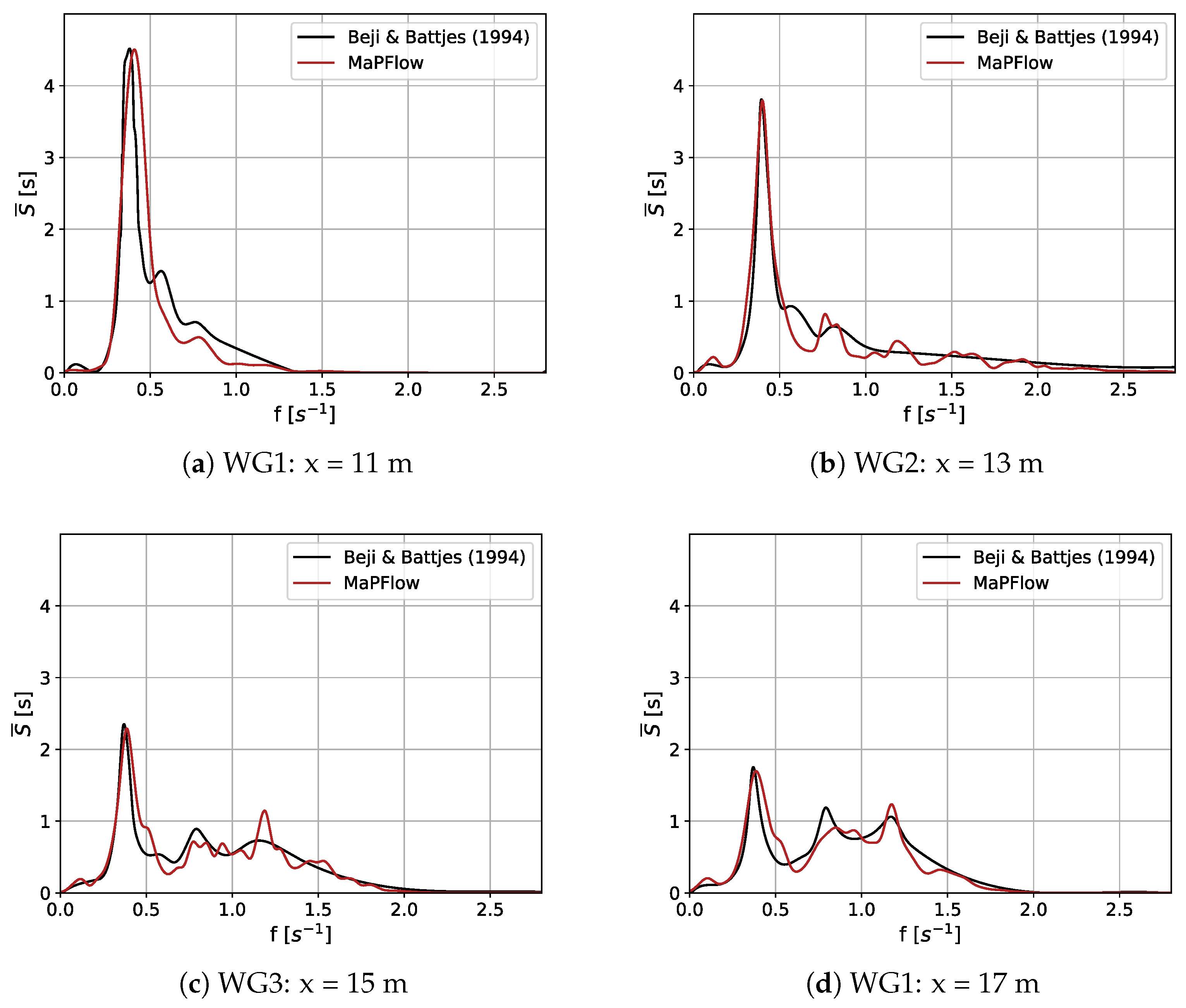
In this section, the developed numerical model is implemented to study the transformation and spectral evolution of irregular waves over a submerged breaker bar. A schematic approach of the numerical wave tank is shown in Figure 5, which emulates the physical wave tank of the experimental work of Beji and Battjes [38], against which the numerical results are also compared. The beach that is used in the experiment for the damping of the waves is omitted here, as it is replaced with the forcing zone.

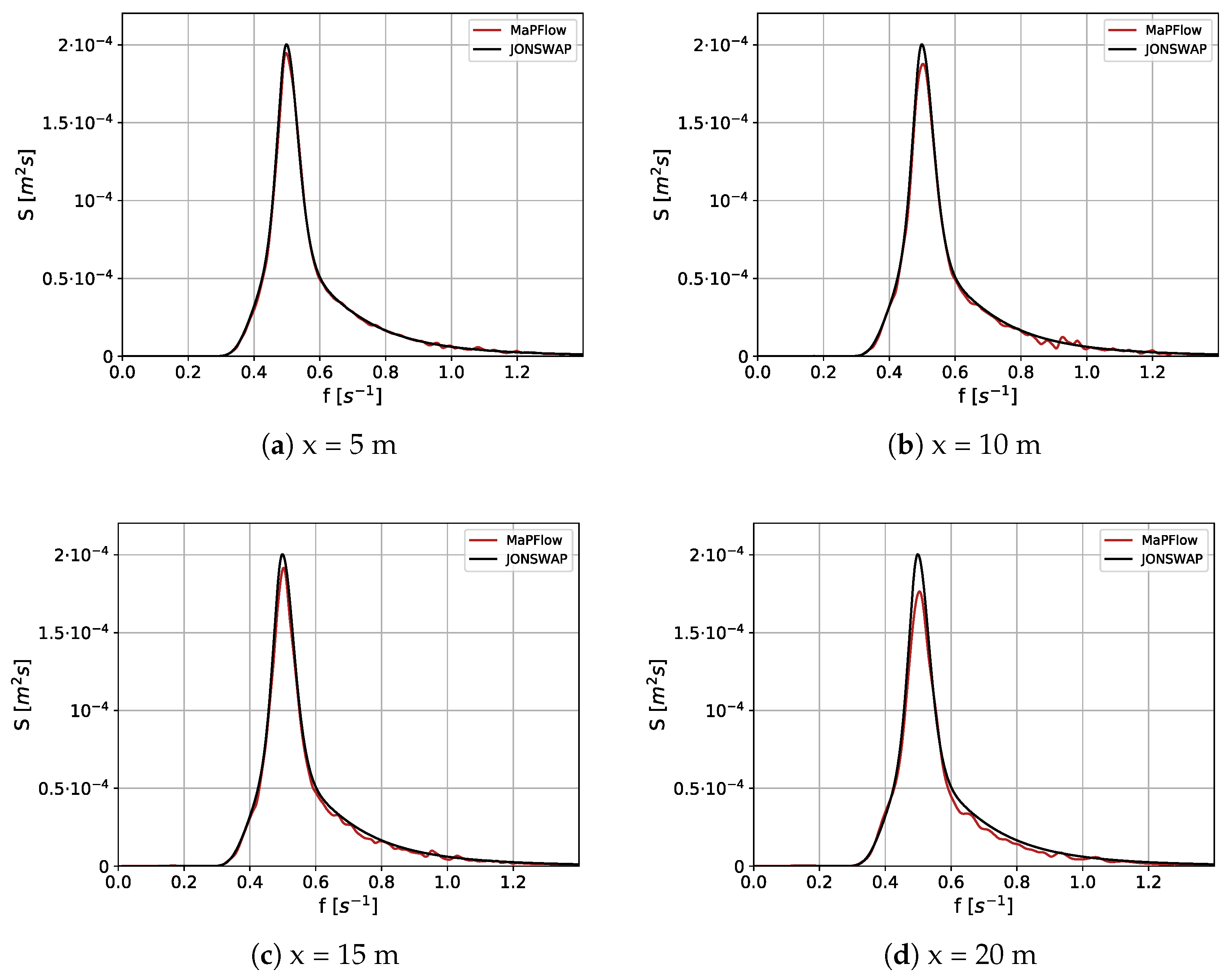
The positions of the wave gauges are chosen to coincide with the experimental gauges for which spectral density results are provided, and they are $x_{WG1}=11$ m, $x_{WG2}=13$ m, $x_{WG3}=15$ m and $x_{WG4}=17$ m. Moreover, two different irregular waves are generated from a JONSWAP-type spectrum, with peak periods of $T_p=2.5$ s and $T_p=1$ s and significant wave heights of $H_s=0.029$ m and $H_s=0.041$ m, respectively. Following the terminology of the work of Beji and Battjes, the first wave pattern is characterized as long waves due to their relatively large wavelength, and the second as short waves.

Regarding the timestep, $dt=T_p/800$ was considered adequate to thoroughly capture the wave transformations, while as for mesh selection, a grid with a uniform cell size in the flat-bottom region of $d{x}_1=0.015$ m, which becomes denser and reaches $d{x}_2=0.01$ m in the region of the bar was created for long waves. However, in order to maintain the philosophy that connects grid properties with the wave features, a much finer mesh was constructed in order to satisfy this condition for the short waves, with the aforementioned cell sizes to be $d{x}_1=0.0085$ m and $d{x}_2=0.005$ m. In the vertical direction, the mesh is relatively dense in the vicinity of the free surface, and it gradually coarsens towards the upper boundary and the lower boundary, while it is also denser in the boundary layer region. The grid sizes for the two wave conditions described above were $335·{10}^3$ and $570·{10}^3$ cells, respectively.

On what concerns turbulence modelling, the Stabilized $k-\omega$ SST model discussed above was used with ${\lambda }_2=0.05$, as prescribed by Larsen and Fuhrman. It should also be clarified that the time history of the free surface elevation in the four gauges does not match the one in the experiment due to a lack of data for the phase angle distribution. Therefore, the soundness of the results is based on the principle that irregular waves generated from the same spectrum will contain the same amount of energy. The number of generated wave components was $N=120$, with a frequency interval of $\Delta f\approx 0.0092$ s⁻¹.

5.1.1. Long Waves

In Figure 6, the normalized energy density spectrum of the simulated long waves in the four stations of interest is presented. The normalization is made so that the area below the spectrum is equal to unity, and it allows direct comparison between spectra for different wave conditions. In the first gauge, which is located on the upslope side of the bar, the spectral energy has increased due to shoaling, and the spectrum has started becoming broader. In the second station, which is located in the horizontal crest of the bar, a decrease in the height of the peak is noticed and higher harmonics have been generated with spectral density spreading towards them in a way that the total amount of energy is maintained. According to Beji and Battjes, that horizontal region plays a significant role in the transfer of energy to higher harmonics, as it creates a non-dispersive regime for the wave. Hence, that process further occurs in the next station, which is also at the top of the breaker bar, with a quite large portion of energy being distributed to higher frequencies. Finally, in the last gauge, which is located on the downslope side of the bar and the de-shoaling process is dominant and the formation of secondary peaks is observed, while the initial spectral peak decreases further. In that region, wave decomposition takes place, from waves of a certain amplitude into several smaller amplitude waves of similar frequencies, and the spectral shape takes its final form from a narrow-banded to a broad-banded spectrum. From a numerical point of view, this process facilitates the damping of the propagating waves before they reach the boundary of the domain.

The simulated results are generally in good agreement with the experimental, and thus, MaPFlow seems to capture the dispersive and shoaling phenomena of the irregular waves. A quite significant deviation is depicted in the region of shoaling (in the first subfigure), which is also observed by Aggarwal et al. [15]. A reason for that might be the selected means of spectral density estimation as, in the present work, the Welch Method was used for spectral estimation, which differs from the method that was used in the experiment. Apart from that, the reallocation of the spectral energy to the different frequency ranges is captured accurately, and the formation of the secondary peaks is also evident.

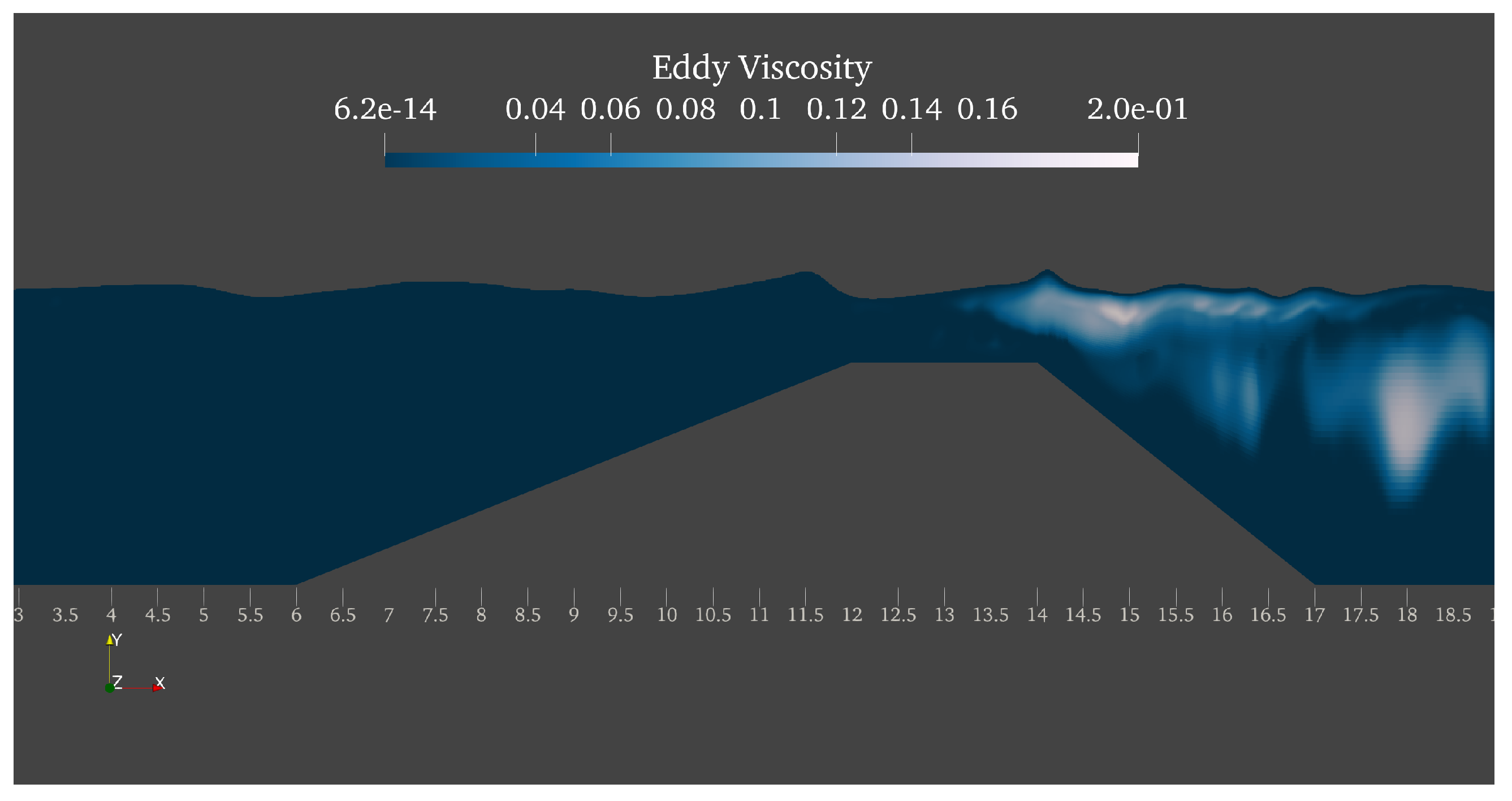
Finally, the eddy viscosity for the case of the long waves is presented in Figure 7. Due to the random character of the propagating waves, the evolution of this variable in time is also chaotic and random. However, the success of the Stabilized $k-\omega$ SST model for the simulation of irregular wave shoaling is quite evident when observing that there is no turbulence production in the region before the bar, while the turbulent viscosity tends to fade during the de-shoaling process.

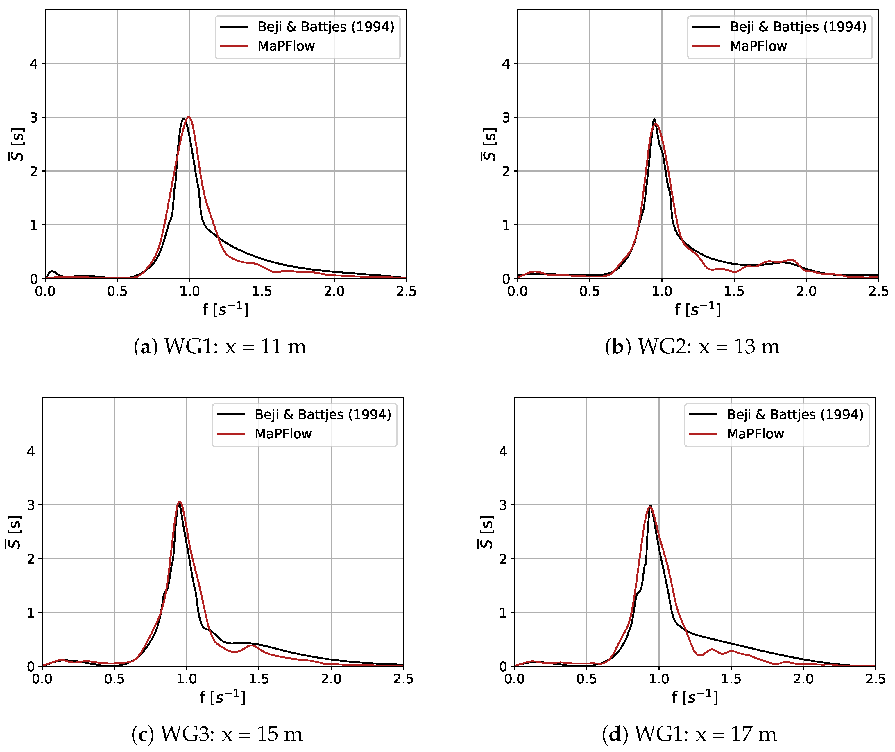
5.1.2. Short Waves

In Figure 8, the normalized energy density spectrum of the simulated short waves in the four stations of interest is presented. In contrast with the long waves, the spectral evolution, in this case, shows shape reformations on a much smaller scale, whereas higher harmonics are not induced on a primary base. This feature is captured well by MaPFlow, and the numerical spectrum maintains its initial narrow-banded shape, similar to the experiment.

The contour plot of the turbulent dynamic viscosity is also presented for the short waves in Figure 9. The trend that is observed in both wave cases is the fact that the emergence of turbulence is strictly located in the region after the bar. Nevertheless, in the short wave simulation, the eddy viscosity is considerably limited in terms of ${\mu }_t$ values, as well as the area of presence, which may be explained by the also limited redistribution of spectral energy to adjacent frequencies.

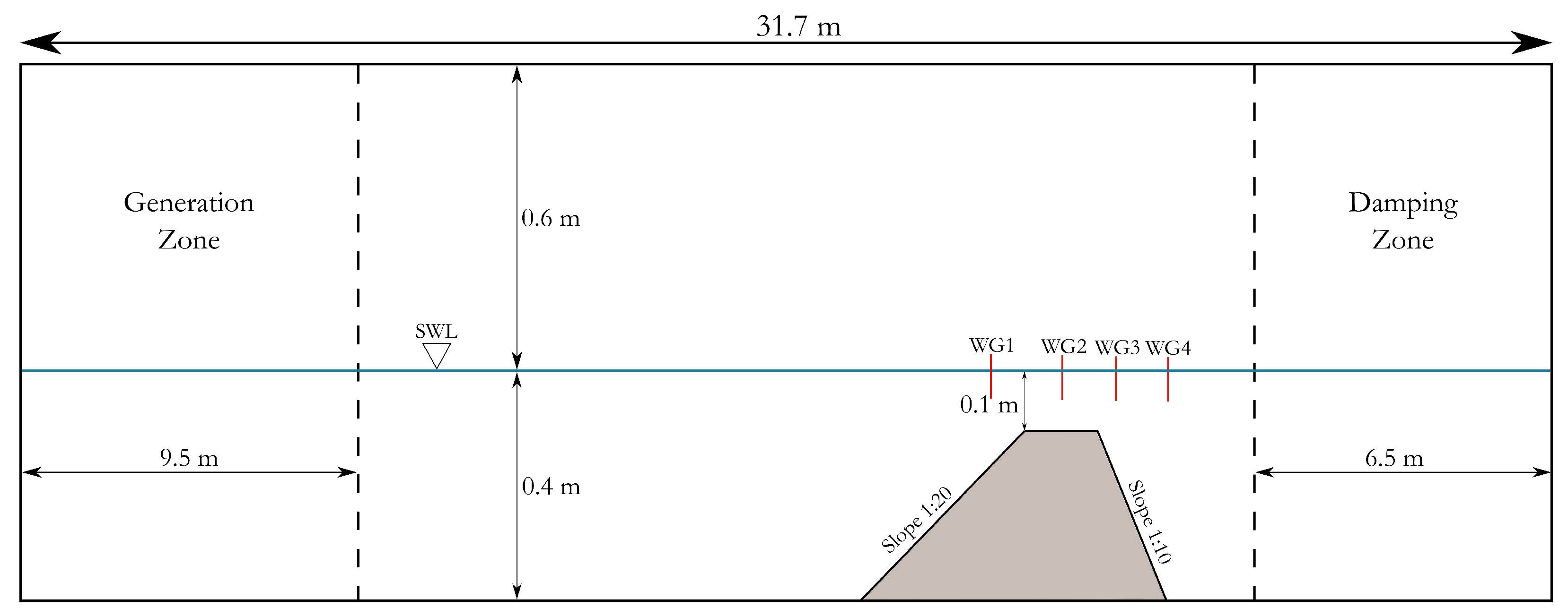
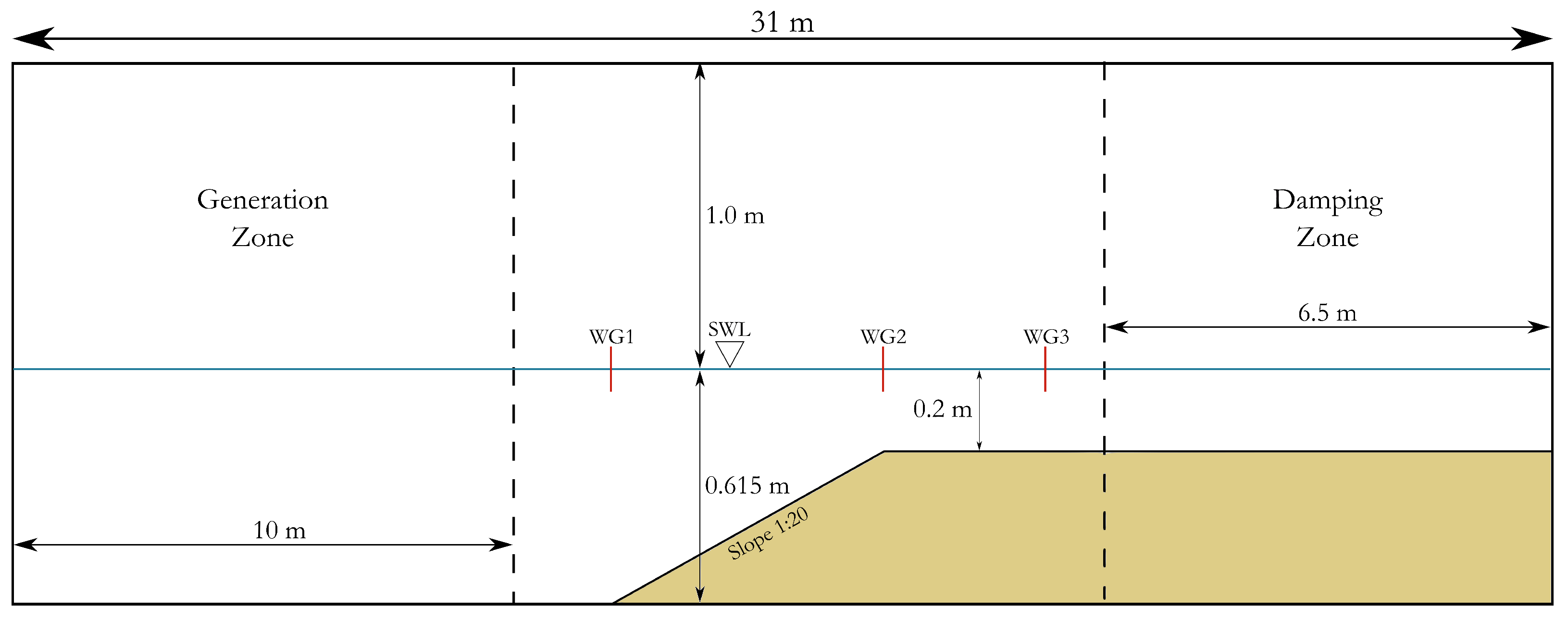
5.2. Piecewise Sloped Seabed

The analysis of the previous section has been conducted using an arbitrary phase angle distribution, and the soundness of the comparison of the results is derived from the fact that both the experimental and numerical irregular waves have been generated according to the same exact spectrum. On the contrary, in this section, the Free Surface Reconstruction Algorithm [39] is used in order to attempt to reproduce the exact free-surface time history of the experiments of Adytia et al. [40] and assess whether the numerical results are in accordance with the experimental wave transformation. A similar approach for the generation of phase-accurate irregular waves and their propagation over the breaker bar of Beji and Battjes [38] can be found in [41].

The numerical wave tank under consideration is presented in Figure 10, and the wave spectrum is of JONSWAP-type with a peak period of $T_p=2.5$ s and a significant wave height of $H_s=0.2$ m. The locations of the wave gauges are identical to the experimental stations at $x_{WG1}=13.65$ m, $x_{WG2}=21.98$ m and $x_{WG3}=24$ m.

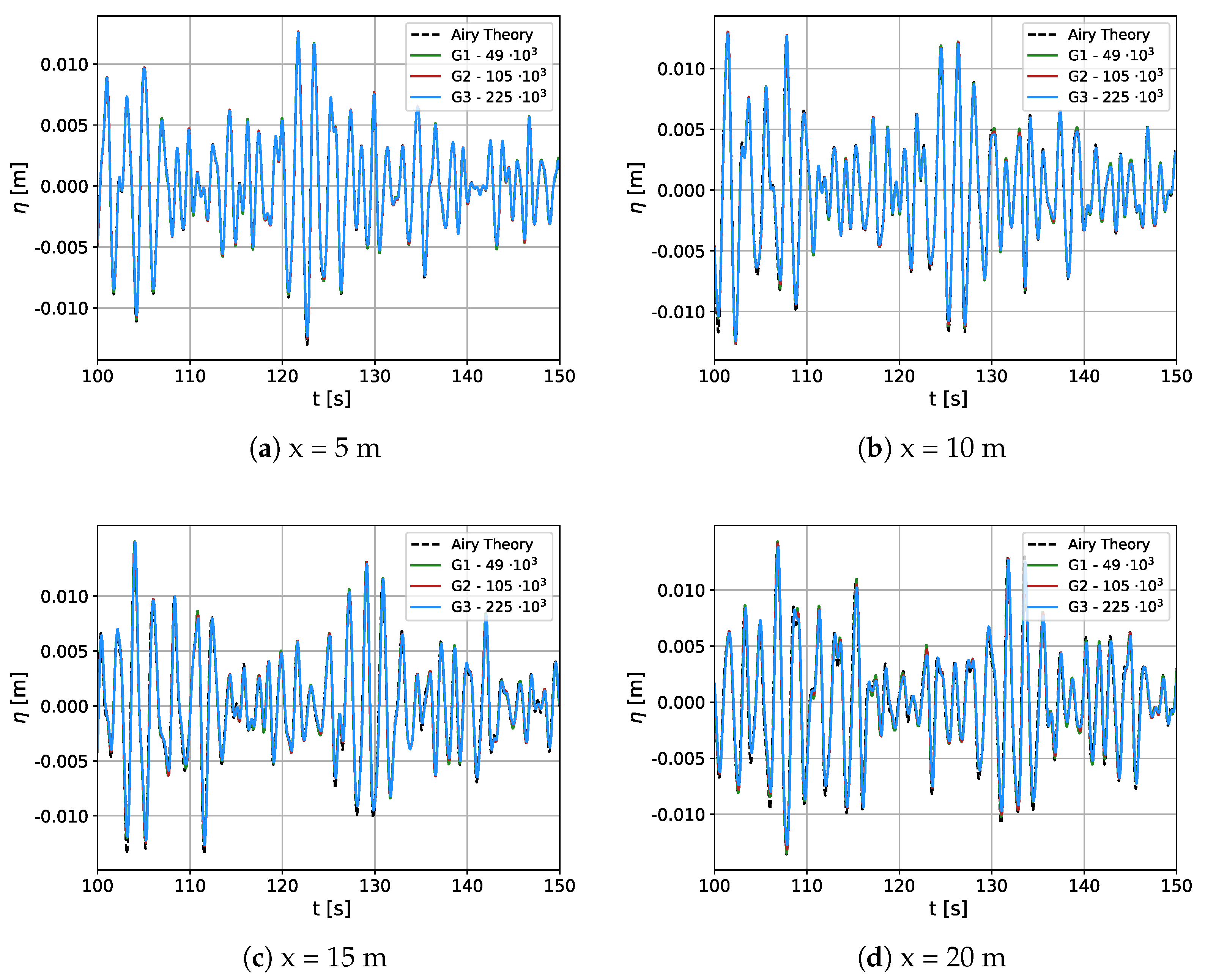
In this case, the breaking is much stronger than the previous since the ratio of the significant wave height to the depth at the most shallow point is $H_s/d=1$. Thus, the starting point of the analysis consists of a grid and timestep independence study. Three grid resolutions of ascending order of refinement were examined, the features of which are shown in

Table 2. Grid resolutions for the case of irregular wave propagation over the sloped bottom.

	Nodes	Cells per ${\mathit{H}}_{\mathit{s}}$	${\mathit{d}\mathit{x}}_1$ (m)	${\mathit{d}\mathit{x}}_2$ (m)
G1	140000	18	0.03	0.02
G2	240000	28	0.02	0.01
G3	356000	34	0.015	0.075

. The term $d{x}_1$ denotes the uniform cell size in the x-direction in the area of the incident spectrum, where the depth is equal to $0.615$ m, while $d{x}_2$ is the cell size in the flat region after the slope.

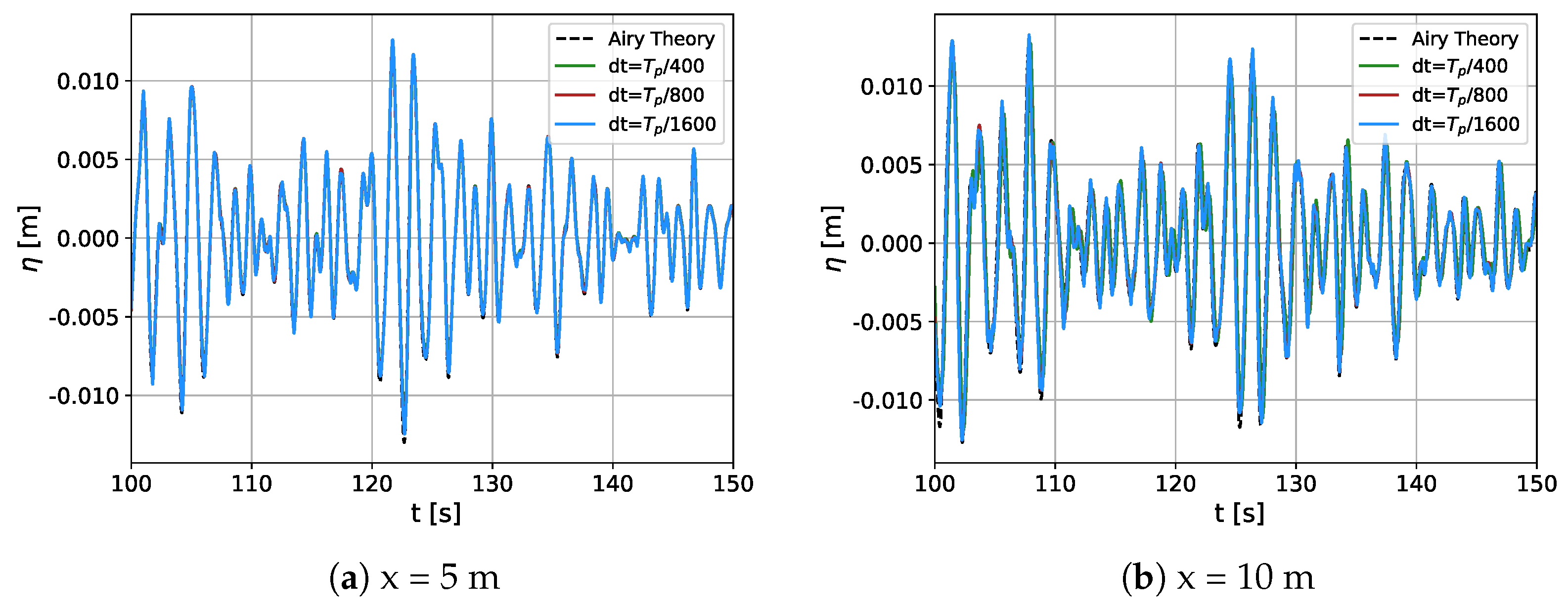
The grid resolution $G2$, with a timestep of $dt=T_p/2000$, was found to be highly accurate and computationally affordable, so for this computational domain, the simulation was carried out for the timesteps $dt=T_p/1000,T_p/4000$ (see

Table 3. Reduction in $E_{rms}$ for the three gauge positions relative to the previous grid/timestep selection (%).

	WG1	WG2	WG3
G1	-	-	-
G2	0.085	0.387	0.931
G3	0.007	0.154	1.047
$T_p/1000$	-	-	-
$T_p/2000$	0.405	2.449	4.129
$T_p/4000$	0.157	0.944	3.385

). A significant increase in the accuracy level was observed in the case of $dt=T_p/2000$, in comparison with the respective increase for $dt=T_p/4000$. Thus, the analysis that follows was conducted using the grid resolution $G2$ and a timestep of $dt=T_p/2000$. Similar to the previous case, due to a more effective representation of the eddy viscosity and turbulent kinetic energy field, the Stabilized $k-\omega$ SST model was chosen for the illustration of the final results. The number of generated wave components was set to $N=100$, with a frequency interval of $\Delta f\approx 0.011s^{-1}$.

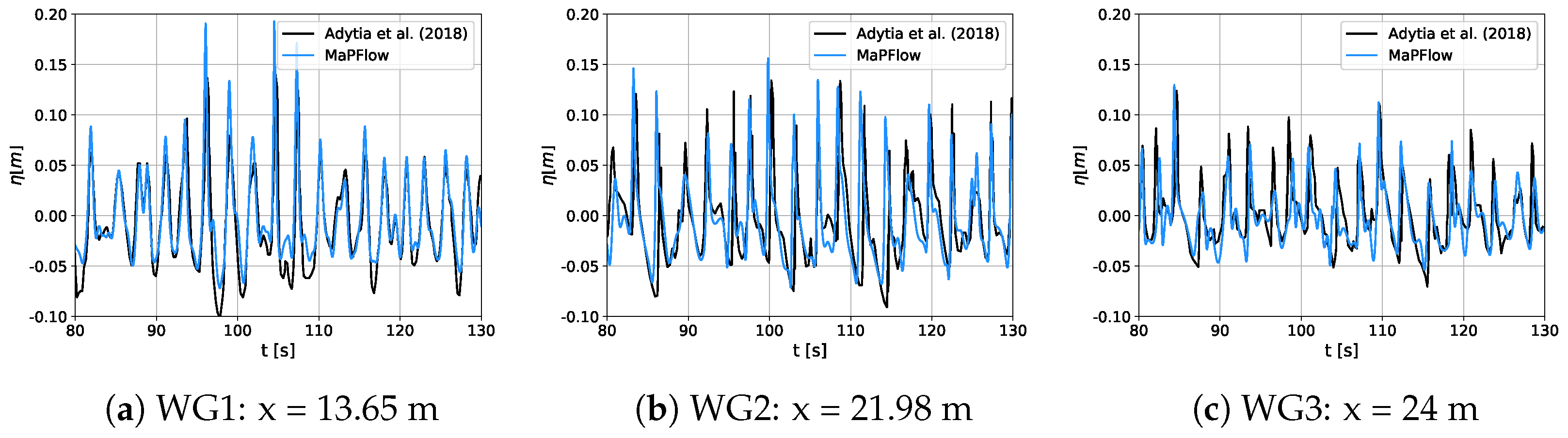
In Figure 11, the reproduced free surface elevation history for the three stations is presented against the experimental results. The first subfigure corresponds to the location where the slope begins and depicts the time history used for the free surface reconstruction. The accuracy of the reconstruction is quite satisfactory; however, several discrepancies are observed in the troughs and crests. The reason for these discrepancies is that the linear Free Surface Reconstruction Algorithm was adopted, and it was mentioned as one of the method’s limitations in the study of Grilli et al. [39]. In the second and third subfigures, the wave transformation and breaking are depicted, and the results are very promising. Considering the inherent error of the FSRA method, it is evident that the wave’s transformation due to shoaling and eventually breaking follows the general trend of the experimental results, despite this relative error. The fact that the elevations follow the periodic profile of the experimental irregular wave highlights the ability of MaPFlow not only to capture the dispersive but also the shoaling phenomena of the problem.

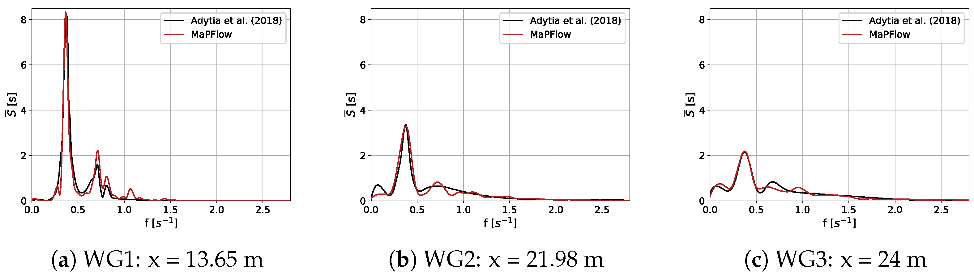
In Figure 12, the spectral evolution of the reconstructed irregular wave along the three stations and in normalized form is presented. In the first gauge, where the incident spectrum is illustrated, apart from the primary peak at the respective frequency, a spread of energy in higher frequencies is observed. In the numerical spectrum, the formation of a secondary peak is also observed but on a smaller scale than the experimental results. This is probably caused by the effect of the seabed on the propagation of the irregular waves since the significant wave height is relatively large compared to the still water depth. In contrast with the previous case, where essentially non-breaking waves were considered, an appreciable portion of energy is lost here due to breaking. This fact can be graphically evaluated by the significant reduction in the area under the spectrum between the second and first gauges. In the last station, which is in the flat bottom area after the slope, further reduction in the wave energy is observed due to the strong interaction of the wave with the seabed topography.

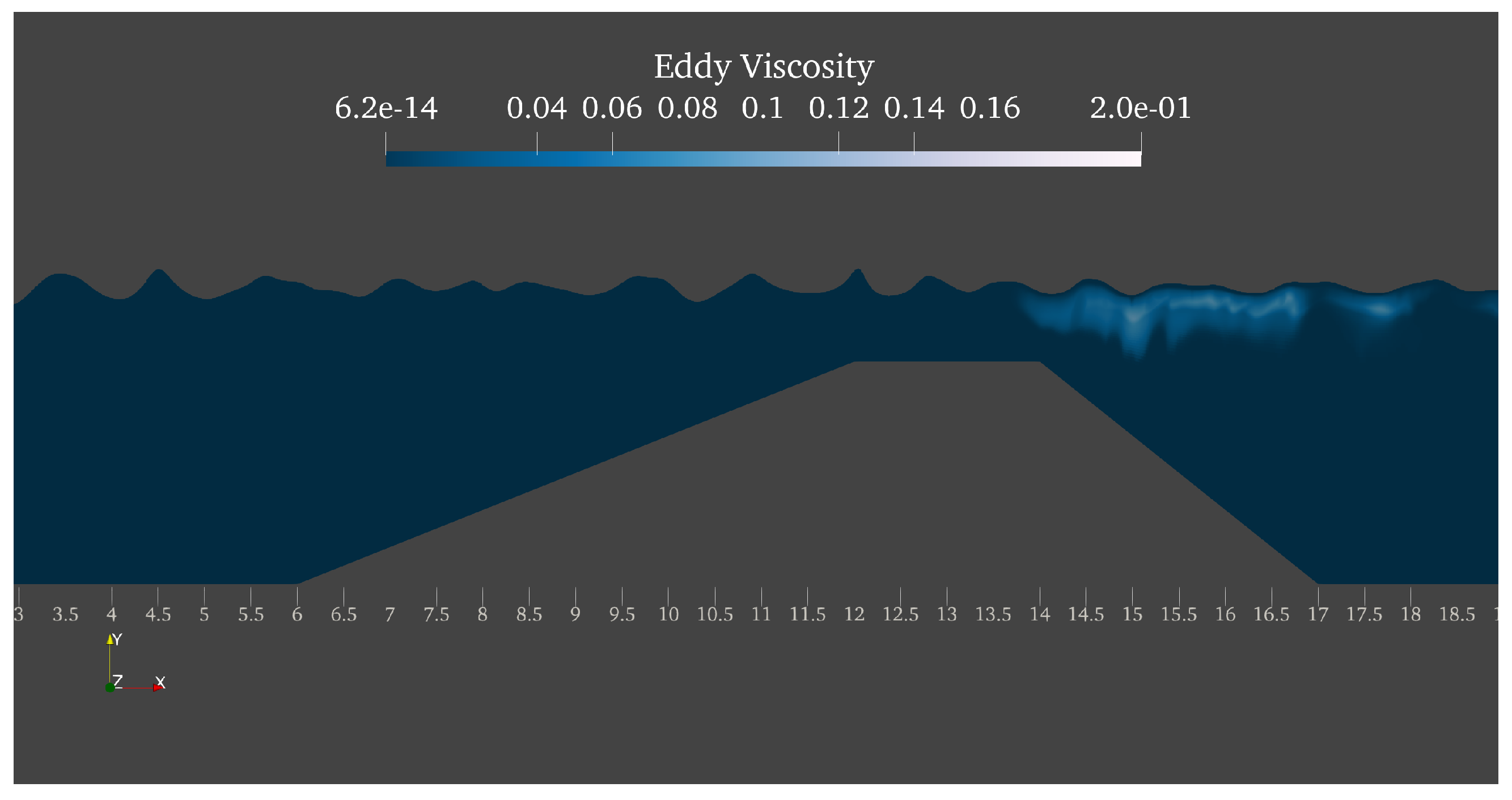
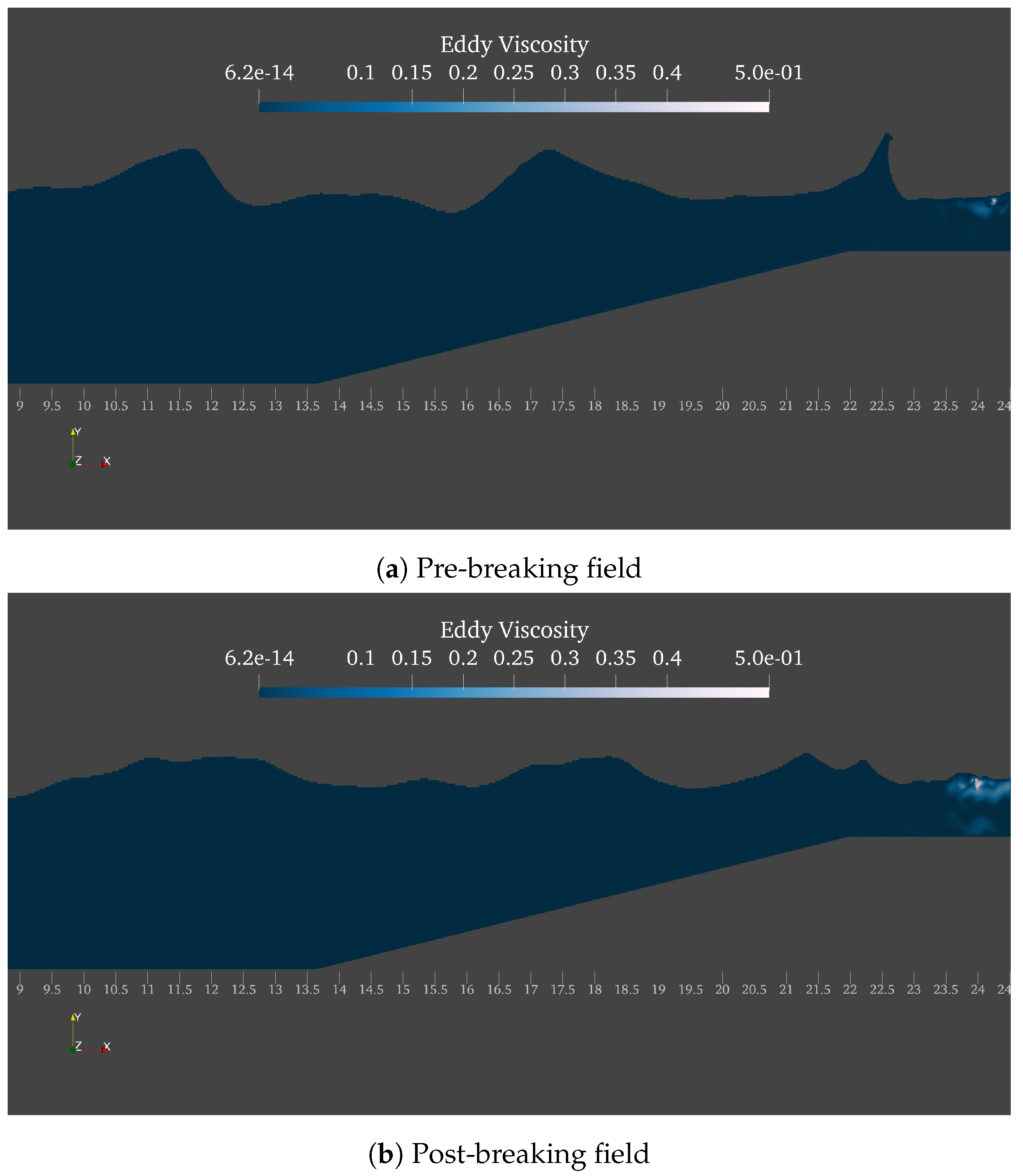
In Figure 13, snapshots of the eddy viscosity in the region of the slope for a formed plunging wave before breaking, as well as for a post-breaking field, are presented. The effect of the stabilization technique is also evident here and can be extended to the case of irregular wave breaking. In particular, in the region where the wave propagates without deformations, no turbulence production is observed, whereas it is mostly generated after the end of the slope, where the breaking tends to occur, and the surf zone is formed. Furthermore, a qualitative aspect that indicates the applicability of this model to irregular wave breaking is the fact that prior to the breaking of the plunging peak (first subfigure), limited turbulence generation is present. On the contrary, after the breaking onset (second subfigure), the turbulence generation mechanisms are activated, and the presence of the eddy viscosity is more intense in the aforementioned region. A quantitative approach to this issue, including the comparison with experimental results, is necessary for further validation of this turbulence model in irregular domains, as well as for the proper calibration of the parameter ${\lambda }_2$; thus, further research is recommended.

6. Conclusions

In conclusion, the present work constitutes a fully-featured approach to modelling irregular wave breaking and addresses several existing issues. First and foremost, an artificial compressibility approach for modelling free-surface flows has been tested regarding its ability to capture irregular wave transformations. The positive attributes that render this approach a good alternative for free-surface flow simulations is that it solves a single system of equations in a coupled manner. Therefore, the occurrence of disturbances, such as spurious air velocities, which are present in pressure-correction methods, is prevented.

Under that scope, an efficient and accurate framework for the generation of irregular waves in a numerical wave tank is adopted, which constructs the desired wave pattern from a given energy density spectrum. For the demonstration of the fidelity of the solver, as well as for the validation of the aforementioned method, the test case of the propagation of irregular waves over a breaker bar is considered. For both long and short waves, the numerical results seem to be in good agreement with the experimental results of Beji and Battjes. For further investigation of the problem, the case of irregular wave propagation over a piecewise linear seabed was considered, through which the ability of the solver to effectively capture the time history of the wave transformation was highlighted.

Furthermore, the problem of turbulence overproduction that is frequently observed in breaking wave simulations is addressed. Precisely, the Stabilized $k-\omega$ SST model is employed, which seems to provide rational results regarding the turbulent regime of wave breaking. Thus, through this work, an extension of the applicability of this particular turbulence model to the domain of irregular waves is made.