Article

Finding Closure Models to Match the Time Evolution of Coarse Grained 2D Turbulence Flows Using Machine Learning

Department of Mechanical Engineering, Johns Hopkins University, Baltimore, MD 21218, USA
*
Author to whom correspondence should be addressed.
Fluids 2022, 7(5), 154; https://doi.org/10.3390/fluids7050154
Submission received: 15 March 2022 / Revised: 22 April 2022 / Accepted: 25 April 2022 / Published: 27 April 2022
(This article belongs to the Special Issue Modelling and Simulation of Turbulent Flows)

Abstract

:
Machine learning is used to develop closure terms for coarse grained model of two-dimensional turbulent flow directly from the coarse grained data by ensuring that the coarse-grained flow evolves in the correct way, with no need for the exact form of the filters or an explicit expression of the subgrid terms. The closure terms are calculated to match the time evolution of the coarse field and related to the average flow using a Neural Network with a relatively simple structure. The time dependent coarse grained flow field is generated by filtering fully resolved results and the predicted coarse field evolution agrees well with the filtered results in terms of instantaneous vorticity field in the short term and statistical quantities (energy spectrum, structure function and enstropy) in the long term, both for the flow used to learn the closure terms and for flows not used for the learning. This work shows the potential of using data-driven method to predict the time evolution of the large scales, in a complex situation where the closure terms may not have an explicit expression and the original fully resolved field is not available.

1. Introduction

Direct Numerical Simulations (DNS) where every spatial and temporal scale in turbulent flows is fully resolved usually require fine grids and long computational times and are therefore too computationally intensive for most flows of industrial interest. Thus, there is a need for reduced order representations of the flow such as Large Eddy Simulation (LES), which are able to predict some of the statistics by evolving only the large scales using subgrid models to account for the unresolved motion. Generating appropriate subgrid models is still an active area of research and often models perform well for one specific flow but not for others. The classical Smagorinsky model, for example, is too dissipative in wall-bounded flows and prevents laminar flows from transitioning to turbulence [1]. DNS that fully resolves all spatial and temporal scales for moderate Reynolds number flows provides enormous amount of data which has been widely used to assist with the development of subgrid models, usually by matching coefficients in relationships between the subgrid stresses and the coarse flow, proposed by scaling and other considerations. The recent availability of data-driven methods to “automatically” extract correlations from very large data-sets are offering new ways to relate subgrid stresses to the resolved coarse flow. While current focus is mostly on single phase flow, this should be particularly useful for more complex flows, where the details of the subgrid scales are less well known.
A number of researchers have recently explored the use of machine learning to develop reduced order models in fluid mechanics [2,3,4,5,6,7,8,9]. See [10] for a review. Most of the contributions have focused on closure models for Reynolds-Averaged Navier-Stokes (RANS) equations, but some efforts have also been made for LES. Sarghini et al. [11] used a Neural Network (NN) to predict the turbulent viscosity coefficient for the mixed model in a turbulent channel flow. Gamahara et al. [12] modeled the subgrid stress tensor directly using NN for turbulent channel flows, without making any assumption about the model form, but the results did not show obvious advantages over the Smagorinsky model. Beck et al. [13] reported instabilities in an a posteriori test with closure models using Residual Neural Network (RNN), even though a priori test showed a high correlation coefficient. Predicting the turbulent viscosity instead of the subgrid stresses did, however, eliminate the instabilities. Wang et al. [14] included second derivatives of the velocity field as inputs for NN to predicted subgrid stresses, showing a better result than the classical Smagorinsky and the dynamic Smagorinsky models for the energy dissipation. Xie et al. [15] used NN to model the source term, rather than the subgrid stresses in homogeneous isotropic turbulence and while they found a high correlation coefficients (0.99), they had to add artificial diffusion to damp out instabilities. They also extended their modeling to turbulence in compressible flows [16]. We note that while Xie et al. [15] work with the source term, they compute it from the subgrid stresses, rather than finding it directly from the coarse field, as we do. We note that 2D turbulece are of relevance to geophysical and planetary flows, due to the large aspect ratio of these systems, but have also been studied extensively as model problems for highly non-linear systems [17,18]. Maulik and San [19] presented an a priori test using NN models for deconvolution of the 2D turbulent flow field, as well as for 3D homogeneous isotropic turbulence, and turbulence in stratified flow. They extended their work by conducting an a posteriori test for 2D turbulence, but had to truncate the predicted subgrid source terms to suppress instabilities [20].
Ensuring that the large scales evolve in a correct way is the main idea of the subgrid stresses. Traditionally, in LES for single phase flow, the subgrid stress can be calculated exactly by τ S G S = u u ˜ u ˜ u ˜ and, therefore, usually the focus is on modeling the subgrid stress directly. The process of modeling τ S G S and comparing it with the exact results from the DNS simulation is generally referred to as an a priori test. However, the success of an a priori test does not guarantee a correct flow evolution, due to errors originating from filtering, discretization and stability considerations. A different strategy is to ask how the evolution equations of the coarse flow have to be augmented or modified to ensure that the flow evolves correctly. In this case, an a posteriori test is automatically taken care of in the modeling and an a priori test is irrelevant. In the context of closure terms for Reduced Order Models (ROMs), Ahmed et al. [21] refer to this strategy as trajectory regression, where the trajectory of the ROMs are optimized, rather than the model itself. Here we use “trajectory regression”, where the time evolution of the filtered 2D turbulence flow field is optimized, by adjusting a closure term added to the continuum equations, and machine learning used to correlate the closure terms to the resolved variables. The advantage of this strategy is that an exact form of the closure terms, explicit filters or DNS data are not needed since the added terms are adjusted by the machine learning to ensure that the coarse flow evolves correctly. Thus, an a priori test is not needed (although doing so would be straightforward for 2D turbulence using a linear filter). We anticipate that not only can our approach be extended to 3D turbulence, but also to more complex flows where either a highly non-linear filter is used for the coarsening, or when only the coarse flow is available.

2. Method

2.1. The Coarse Field

We conduct fully resolved simulations of an unsteady two dimensional flow and filter the results to produce a coarse grained velocity and pressure fields. The simulations are done using a standard projection method on a regular staggered grid. A second order Runge-Kutta method is used for the time integration, a second order QUICK scheme is used for the advection terms and second order centered approximations are used for all other spatial derivatives. The coarse grained velocity field, denoted by u ˜ , is generated by spatial filtering. Here we use a Gaussian:
G Δ = ( 6 π Δ 2 ) 3 / 2 e x p ( 6 x x 2 Δ 2 ) ,
where Δ is the cutoff length that separates the length scales.
To evolve the coarse field, we add a source term F to the single-phase incompressible Navier-Stokes equations:
u ˜ t + · u ˜ u ˜ = 1 ρ p ˜ + ν 2 u ˜ + F ,
where ρ is the density, p ˜ is the coarse grained pressure field and ν is the kinematic viscosity. We then calculate the source terms so that the time evolution of the coarse grained flow matches the filtered solution:
F = u ˜ t + · u ˜ u ˜ + 1 ρ p ˜ ν 2 u ˜ .
We note that this is different from what is usually done for LES modeling using DNS results, where the subgrid stresses are computed from the fully resolved results. The extra term, F , is intended to ensure that Equation (2) evolves the coarse field correctly. While we have the fully resolved flow field and could thus compute the subgrid stresses directly in the usual way, our motivation is to test an approach applicable to cases where we only have the coarse field.

2.2. Neural Network (NN) Architecture

The key assumption in LES is that the subgrid stresses can be related to the coarse or large scale flow and we assume that the same is true for the source term (even if it is not computed directly as the divergence of the stresses). The source term cannot depend directly on the velocities since we can always add a constant translation based on Galilean invariance, so it must depend on the derivatives of the velocity. For three-dimensional flows, Wang et al. [14] examined the relevance of a number of variables as input for neural network for the subgrid stresses and determined that the first and second derivative of the velocity were most important. Xie et al. [15] determined the source term · τ S G S (which they refer to as the SGS force) using the first derivatives, but included several surrounding spatial points, instead of just the single point under consideration. They found that working with the full source term, rather than the stresses, resulted in a much better agreement with the filtered data. Here, we assume that the source term depends on the local value of the first and second derivatives: u ˜ x , u ˜ y , v ˜ x , 2 u ˜ x 2 , 2 u ˜ x y , 2 u ˜ y 2 and 2 v ˜ x 2 . Only 7 components are needed because of the incompressibility condition. Since the flow is isotropic and without any directional preference, we can use the same expression for the two components F x and F y , since by rotating the coordinate system by 90 in counterclockwise direction, the new “x” axis collapses into the original “y” axis. Thus, we can use the same mapping function for the y component, by projecting the fluid velocities of the original coordinate system onto the rotated coordinate system. Thus,
F x = M u ˜ x , u ˜ y , v ˜ x , 2 u ˜ x 2 , 2 u ˜ x y , 2 u ˜ y 2 , 2 v ˜ x 2 ,
F y = M v ˜ y , v ˜ x , u ˜ y , 2 v ˜ y 2 , 2 v ˜ x y , 2 v ˜ x 2 , 2 u ˜ y 2 ,
where M denotes the function found by the machine learning. In this way we preserve the rotational invariance, are able to use the data for the two components together in one big dataset, and train only once. Siddani et al. [22] also rotated the coordinate system to augment the training dataset, based on the rotational invariance. Ling et al. [2] proposed a neural network architecture with embedded invariance property by constructing an integrity basis for the input tensor.
The Neural Network is a multilayered structure, with a linear vector transformation followed by a nonlinear activation function at each layer, achieving complicated regression from inputs to outputs. Here, we use a Neural Network with a relatively simple structure, containing one input layer with 7 neurons, 3 hidden layers with 20 neurons in each layer, and an output layer with 1 neuron. Neurons in adjacent layers are fully connected to each other. The transformation from layer l to layer l + 1 can be expressed as
Y l + 1 = σ ( W l X l + b l ) ,
where X R m × 1 is the data in layer l, Y R n × 1 is the data in layer l + 1 , W R n × m and b R n × 1 represents the weighting matrix and the bias term that needs to be optimized. σ ( x ) stands for the RELU activation function, σ ( x ) = m a x ( x , 0 ) , used to introduce nonlinearity into the mapping. For effective learning, the input data has been preprocessed in such a way that X 0 = 1 α ( X X m e a n ) , where X m e a n and α are the mean and standard deviation of the raw data. The NN structure is built with Keras in Python 3.7 and the mapping is optimized by stochastic gradient descent method by monitoring the mean square error as the loss function. Based on our experiment, 500 epochs are generally enough for finding the optimum and the loss function does not decrease significantly with a further increase in the number of epochs. We note that while the simple NN structure used here works well, using more sophisticated adaptive activations may speed up the convergence and increase the accuracy of the training [23,24,25].

3. Results and Discussion

To generate a 2D turbulent flow in a doubly periodic domain, we start with four perturbed shear layers that quickly break up by Kelvin-Helmholtz instability into approximately isotropic flow as seen in Figure 1, where the vorticity is shown at two times. The domain size is 2 π × 2 π , resolved by a 2048 × 2048 grid. Due to the inverse energy cascade characteristic of 2D turbulence, small vortices grab each other and form larger ones, as shown in the evolution of the vorticity field. In this case, turbulence energy dissipation rate is ϵ = 2 ν ( S i j ¯ S i j ¯ ) = 0.179 and the Kolmogorov length scale is approximately η k = ( ν 3 / ϵ ) 1 / 4 = 0.009 . The Reynolds number defined by the integral length scale is R e L = u R M S L / ν = 2335 , where u R M S is the RMS velocity u R M S = E k = 3.28 and the integral length scale can be found by L = ( π / 2 u R M S 2 ) E ( k ) k d k = 0.713 . The large eddy turnover time scale is τ L = L / u R M S = 0.22 , and the simulation is run for over 45 large eddy turnover times.

3.1. NN Learning

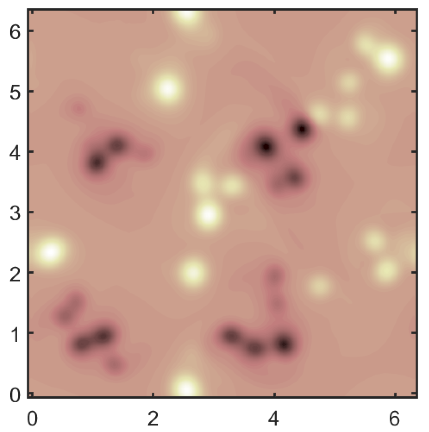
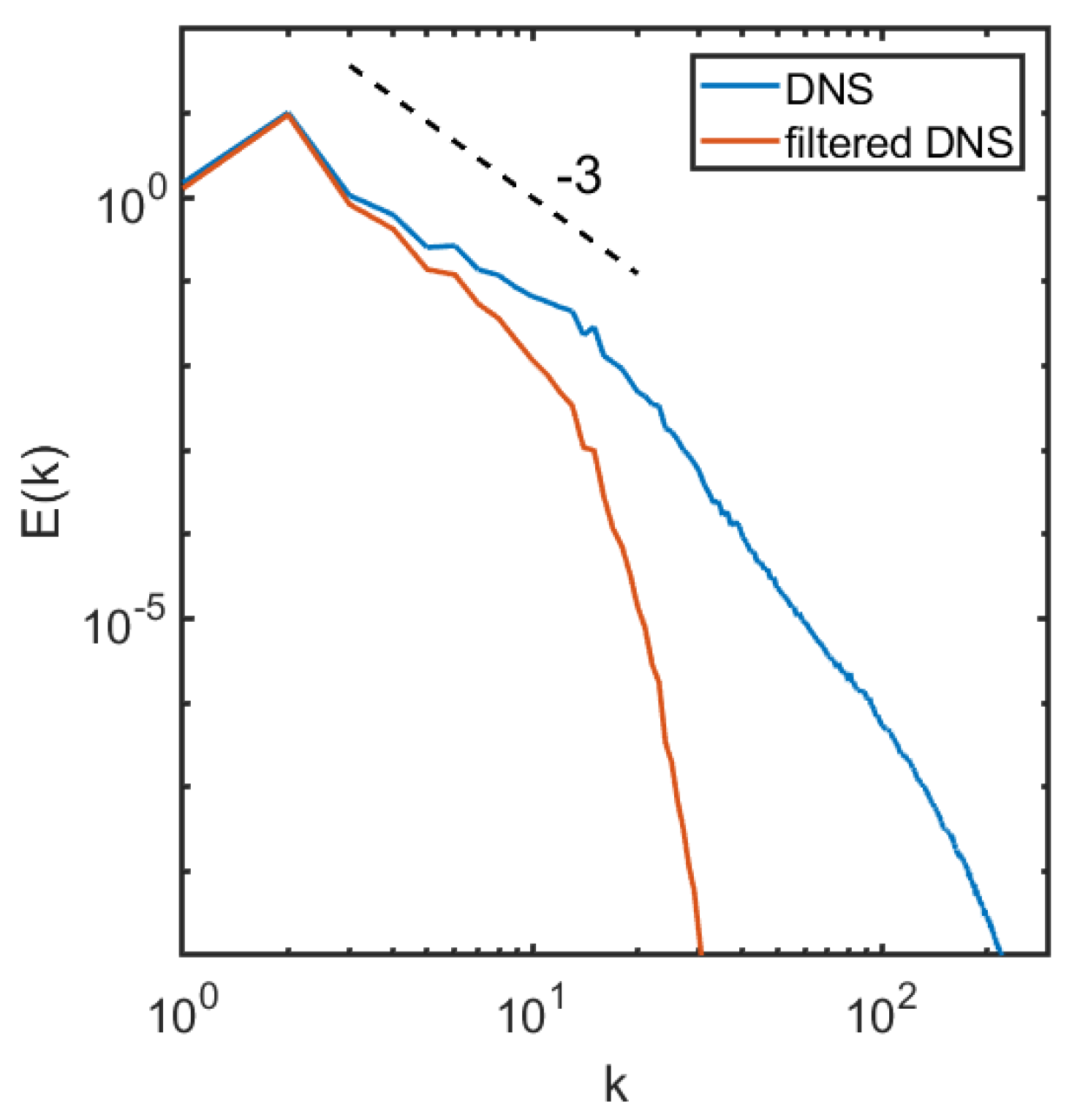
To generate a coarse flow field, we apply a Gaussian filter to the DNS flow field so that the original 2048 × 2048 field is coarsened to 128 × 128 grid points, or Δ c = 16 Δ f , where Δ c and Δ f denote the coarse grid spacing and the fine grid spacing, respectively. The filter width in Equation (1) is chosen to be Δ = 0.4 , which is about half the integral length scale L and much larger than the grid spacing of the coarse mesh ( Δ c = 0.049 ). Note that the filter applied here is more aggressive than that in [19], who used Δ c = 8 Δ f . The filter size is also much larger than the fine grid spacing ( Δ = 130 Δ f ), and more aggressive than in [15] where Δ = 32 Δ f . Figure 2 shows the filtered vorticity field on the 128 × 128 grid. We obtain the 1D energy spectrum E ( k ) = 1 2 | u ^ ( k ) | 2 , where u ^ ( k ) represents the Fourier Transform of the velocity fluctuation field, by taking the Fourier transform of the fluctuation along the x direction and average in the y direction. Doing it in a reversed way (taking the Fourier transform along the y direction and averaging in the x direction) gives similar results. The energy spectrum for the fully resolved DNS solution and the filtered flow are shown in Figure 3. The spectrum shows the classical 3 power law in the inertial range for 2D turbulence [17].
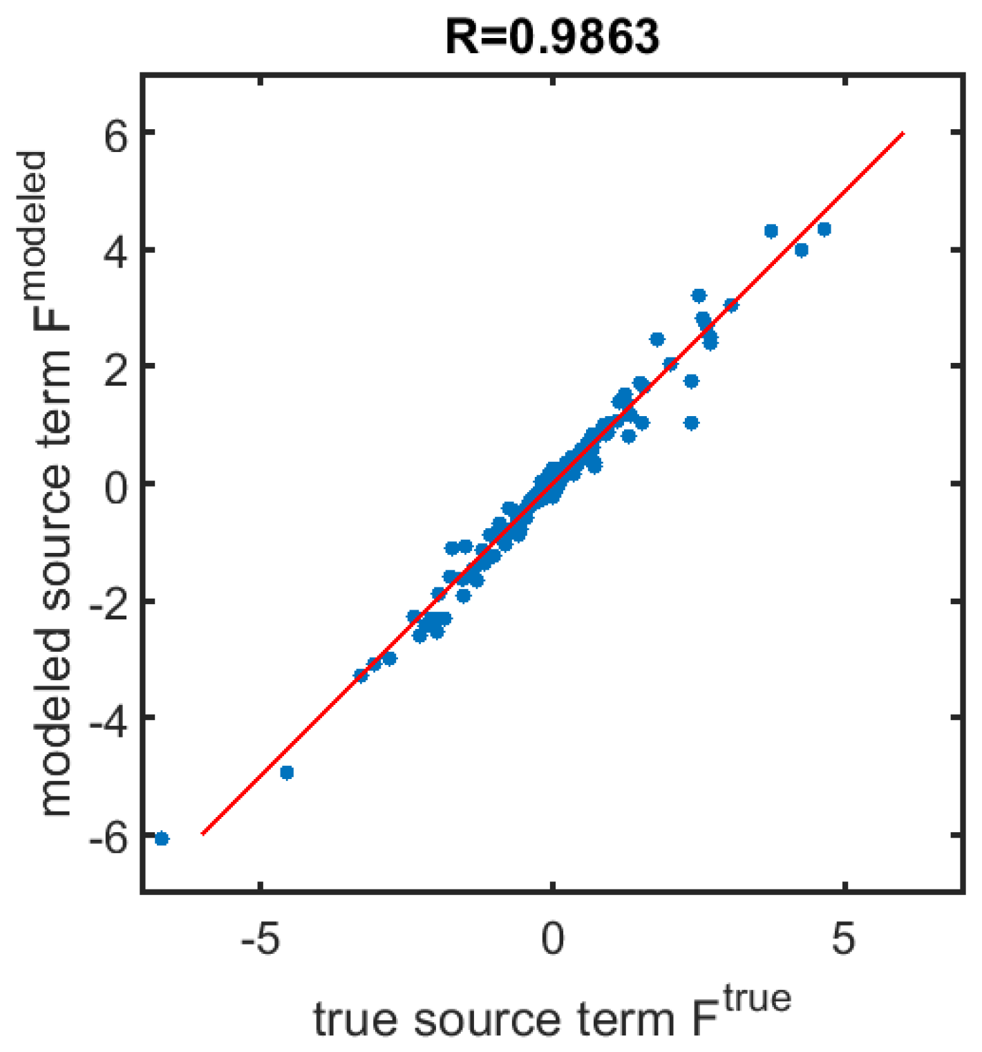
Here, we sample the data every Δ t * = 2.27 from t * = 2.27 to t * = 27.27 for the Neural Network training, giving a total of 12 filtered DNS fields, each containing 128 × 128 data points (total of 393,216 samples by combining data for both components). We calculate the first and second derivatives of the filtered velocity field based on finite difference and use those as the NN inputs based on Equation (4). Before the data was used to train the NN, it was normalized by subtracting the mean and dividing by the standard deviation, enforcing a mean and standard deviation of 0 and 1, respectively. The data is split into a training set (90%) and a validation set (10%) randomly in order to perform a cross-validation. Figure 4 shows the predicted value of one component of the source term versus the true source term computed from the data by Equation (3). The correlation coefficient is shown on the top of the frame. It achieves a value higher than 0.98 after 500 epochs. Increasing the number of epochs, as well as using different initial guesses, has minimal impact on the results. The high correlation coefficient in the cross-validation test is about the same as Xie et al. [15] found and higher than what Wang et al. [14] found (0.7). The NN found here only works for a specific Reynolds number, filter size and relatively homogeneous isotropic 2D turbulent flow, with no solid boundary walls in the domain. In principle, we can use Reynolds number and filter size as inputs for the NN and enlarge the training dataset to include other simulations with different R e and filter sizes, in order to generalize the NN. Our scope, however, is more limited and we only seek to show that we can use machine learning to find the closures if only the coarse fields are available.
The source term coming from the neural network is not a completely smooth function and the noise is sometimes amplified when used in the modified Navier-Stokes equations. To eliminate that we smooth the source term slightly, using a box filter to smooth it over a 5 by 5 stencil on the course grid. Using a Gaussian filter with the same cut-off length as used to coarsen the fully resolved flow also gives similar results. We note that instabilities were also seen in other works [13,15,20]. In order to avoid the numerical instabilities for 2D flows, Maulik ans San [20] forced the subgrid stress to be only dissipative at large scales by truncating the source term, assuming that the small scales only cause dissipation of the kinetic energy. Piomelli et al. [26] pointed out that forward- and backscatter are present in approximately equal amounts in 3D. This was also shown in [20], who found that even in 2D flows about half of the grid points transfer energy from fine scales to large scales. Here, we avoid excluding the backscatter mechanism. Xie et al. [15] prevented instabilities in 3D by including artificial dissipation into the momentum equation to damp out the high frequency fluctuations.

3.2. A Posteriori Tests

Studies of subgrid stresses in LES typically distinguish between an a priori comparison of predicted subgrid stresses with subgrid stresses computed by filtering fully resolved results, and an a posteriori comparison of how well the flow field computed by LES matches the filtered fully resolved results. In our case, where the closure terms are computed directly by matching the coarse grained flow evolution, an a priori test is irrelevant. We are not trying to reproduce the subgrid stresses or the source term computed from the filtered DNS solution, but to ensure that the coarsened field evolves correctly. The a posteriori test on the other hand, where we compare the evolution of the coarse grained field to the evolution of the filtered fully resolved field, is of course the ultimate test.

3.2.1. The Training Data

The purpose of a subgrid model is to ensure that the coarse field reproduces the evolution of the fully resolved field, filtered at each instance in time. Since the flow is highly unsteady and slightly different initial conditions diverge at long times, we do not expect the coarse solution to follow the filtered field exactly, except initially. Thus, we can only do a detailed comparison between the spatial fields at early times and must be content with comparing statistical quantities at later times.
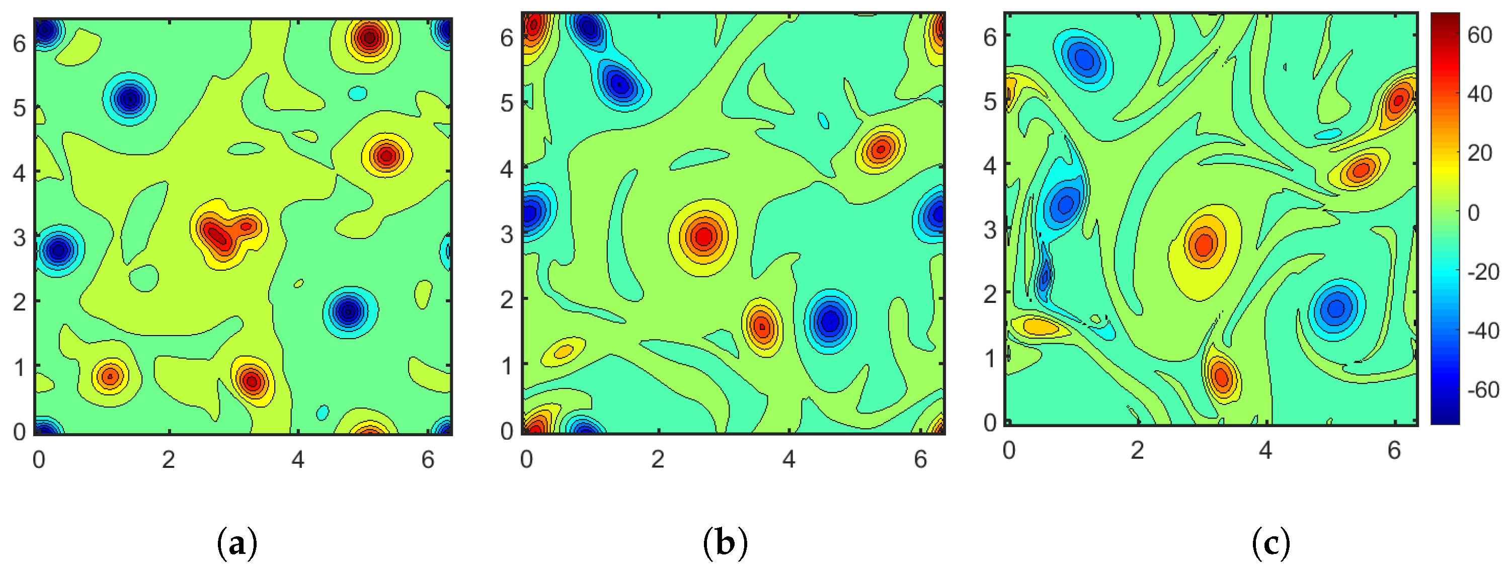
We use the filtered DNS field at t * = 4.55 (Figure 2) as the initial condition for the a posteriori test. The LES uses a 128 × 128 grid, with the NN predicted source terms F m o d e l added on the right hand side of the momentum equation, followed by a slight spatial smoothing of the modeled source term field. We also ran an under-resolved DNS simulation on a 128 × 128 grid for comparison, also with the filtered fully resolved solution at t * = 4.55 as initial conditions. Figure 5 shows the instantaneous vorticity field as found by the filtered DNS, the LES and the under-resolved DNS at t * = 11.36 . The agreement between the filtered DNS and the LES results is reasonably good and the coarse grid solution (under-resolved DNS) is further away from the filtered solution. This suggests that the NN model captures the evolution of the coarse filtered field, at least for the first 6.81 large eddy turnover times.
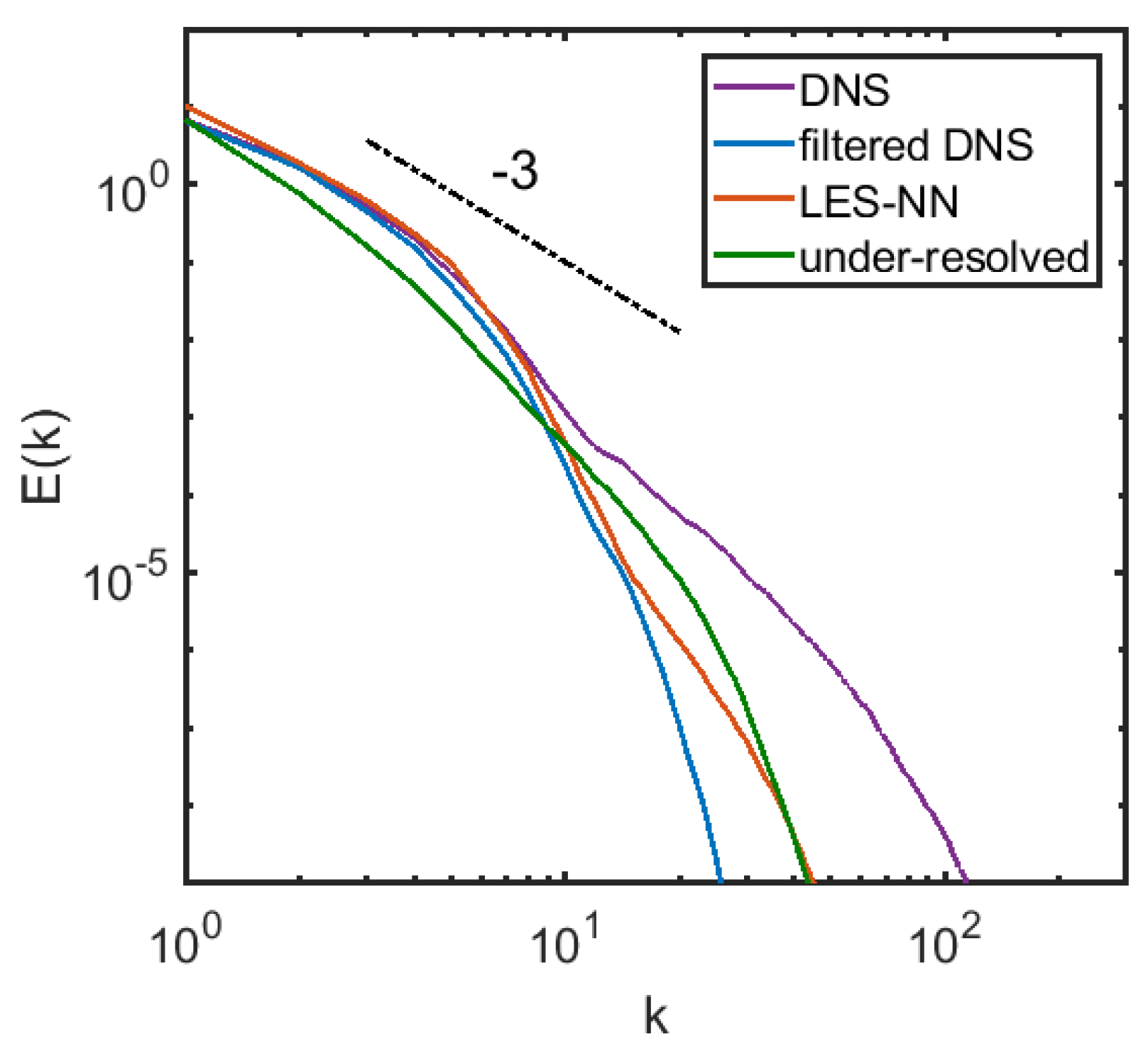
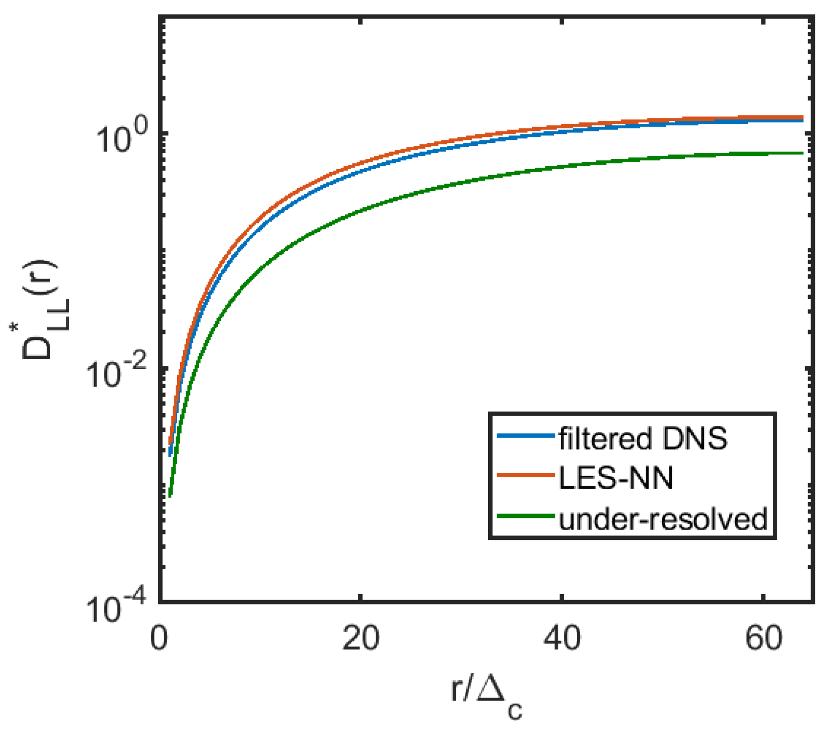
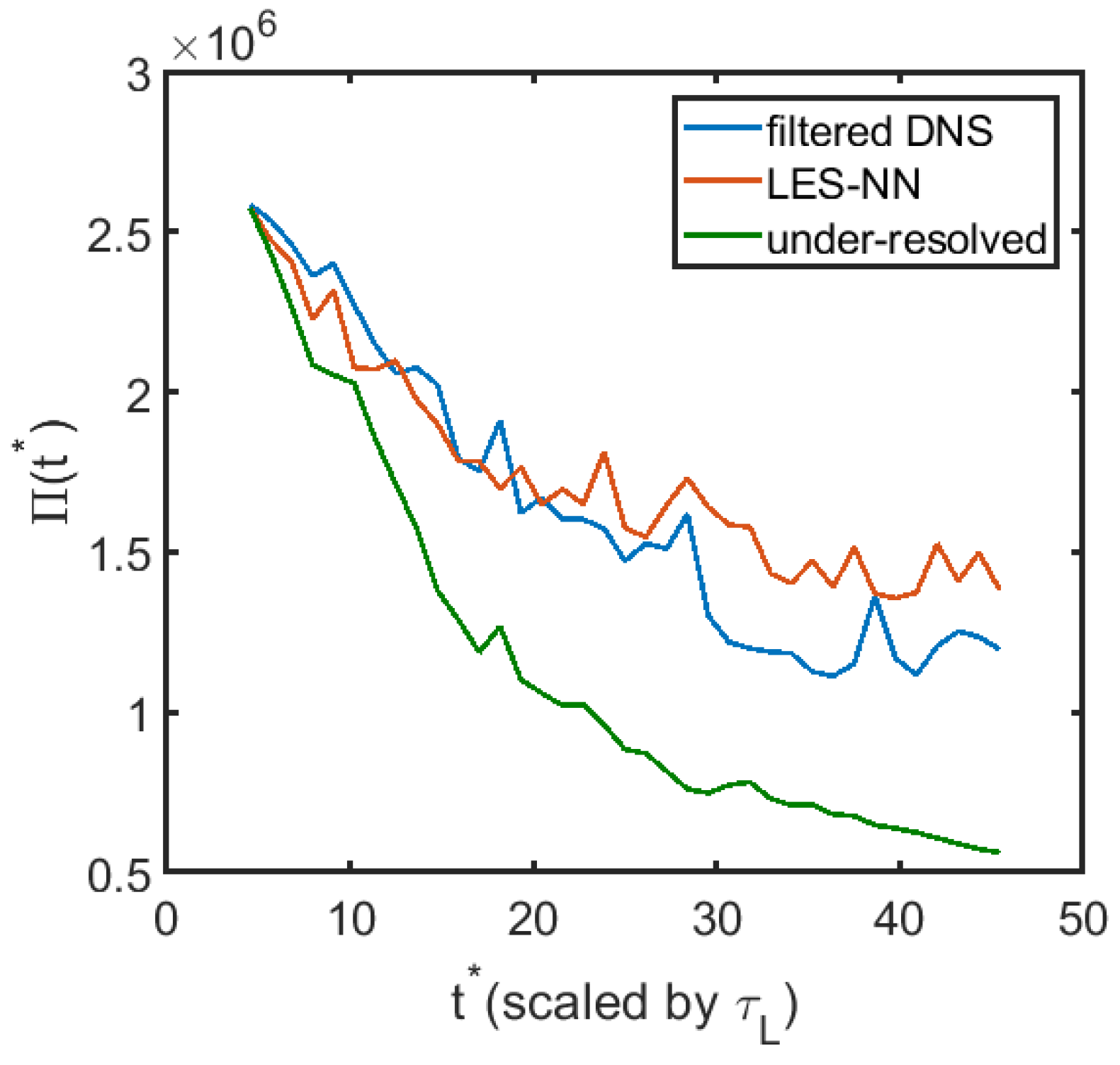
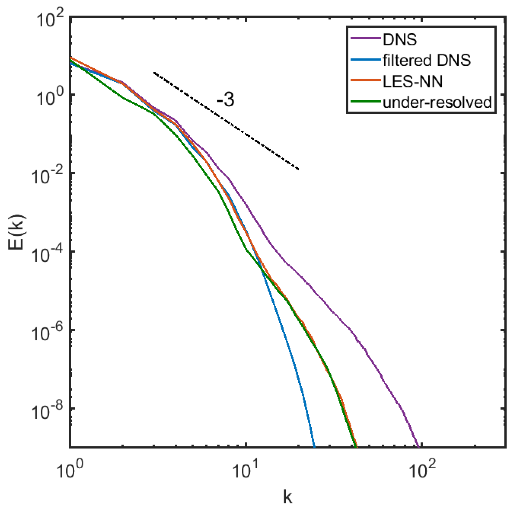
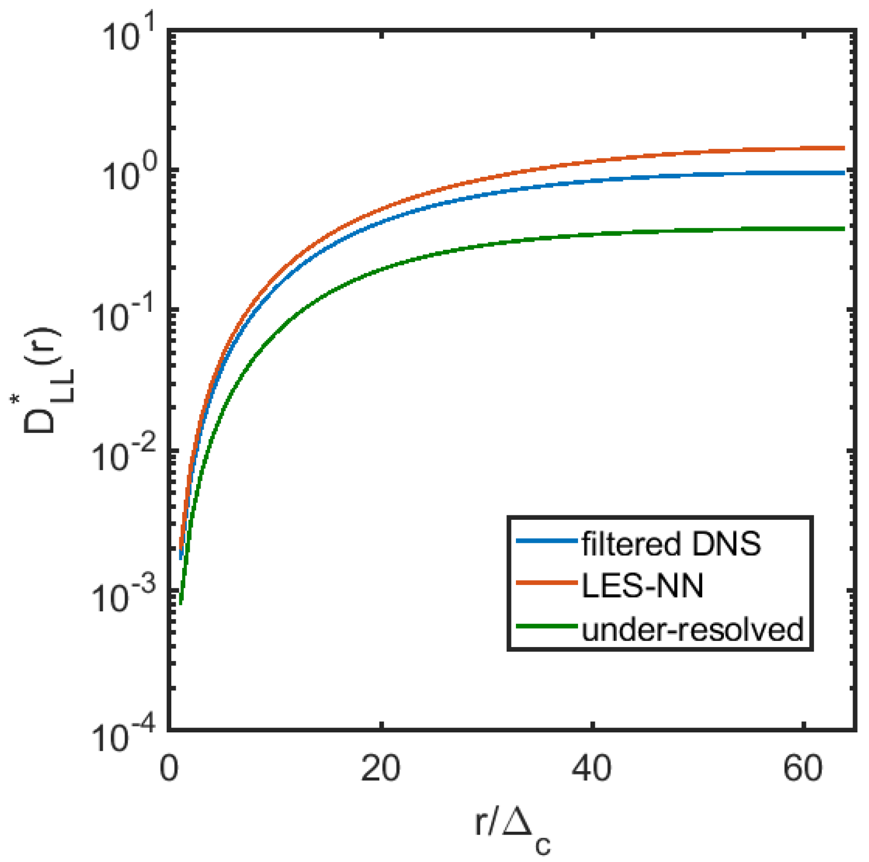
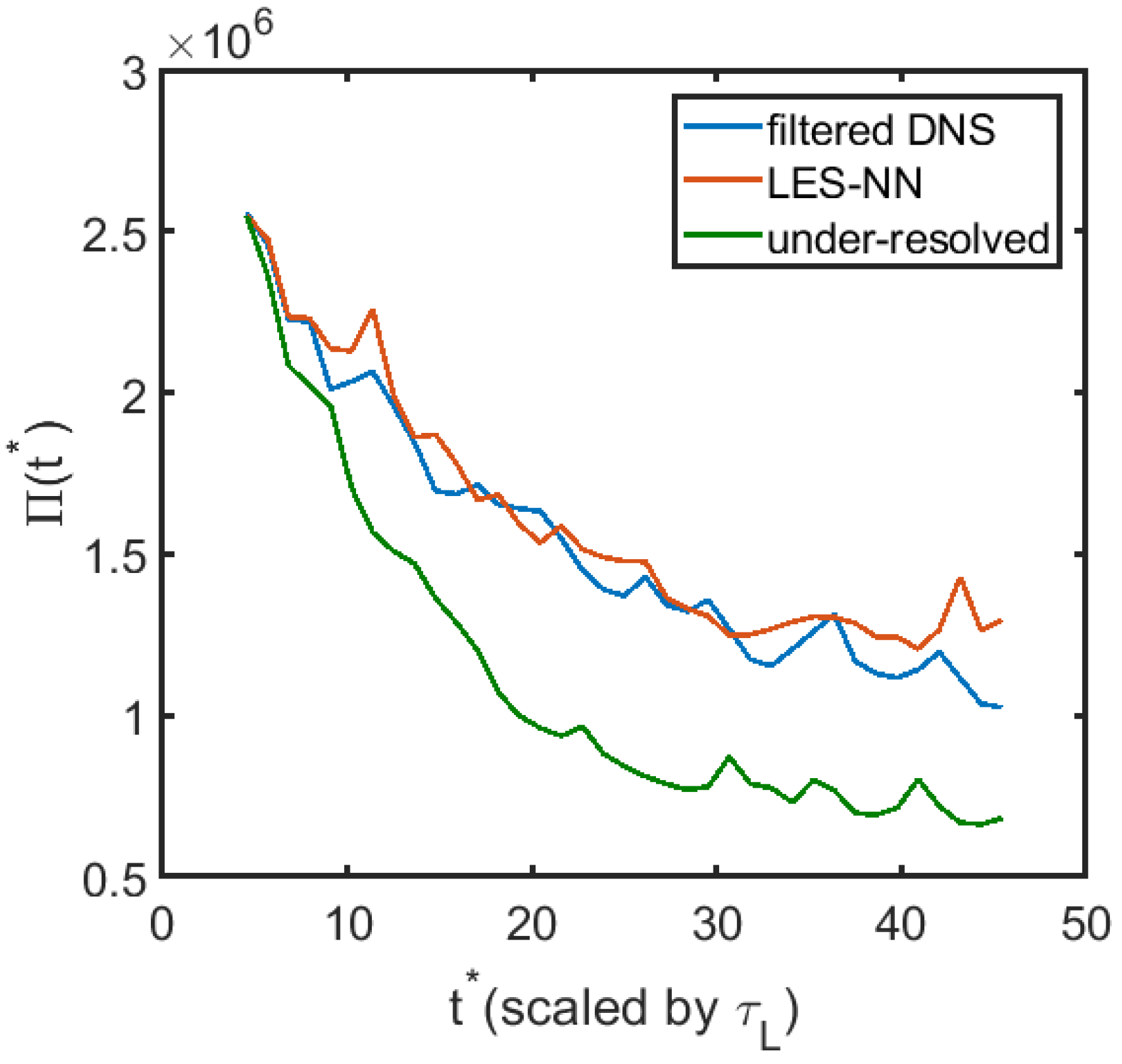
Since it is unrealistic to expect the coarse field obtained by filtering the fully resolved results and the coarse field evolved by the model equations to match completely at long times, we calculate the 1D energy spectrum and the 2nd order structure function for the filtered DNS field, LES field with NN model, and the coarse grid solution with no models. The 1D longitudinal structure function is defined as D L L ( r ) = ( u ( x + r ) u ( x ) ) 2 ¯ , where u denotes the horizontal velocity fluctuation. We average the field at 11 different times and nondimensionalize the structure function by u R M S 2 . Averaging with more samples or at other times does not significantly change the structure function or the 1D spectrum. As shown in Figure 6, the energy spectrum obtained by the NN modeled LES follows the 3 power law well in the inertial range. The coarse grid solution is however, a little bit away from the 3 power law at large scales. Figure 7 shows the 1D 2nd order nondimensional longitudinal structure function versus r / Δ c . The NN modeled LES structure function agrees well with the filtered fully resolved one, and is much closer than the coarse grid solutions. We also plot the enstropy, defined as Π = ω · ω d S , versus time for the three different cases in Figure 8. It can be seen that there is an obvious improvement in matching the enstropy evolution by using the NN modeled LES compared to the under-resolved solution. We note that it takes 25 days on a single Intel core to evolve the DNS solution to t * = 45.46 but only less than half an hour for the NN modeled LES.

3.2.2. Non-Training Data

In the previous section we show that the Neural Network closure model works well in terms of matching both the instantaneous flow field at early times as well as the turbulence statistics at long times for the data used to train the model. Here we apply the model to a different case generated by 4 vertical shear layers separating flows with discontinuous velocities, still on a 2048 × 2048 grid for a domain size of 2 π × 2 π . The Reynolds number, defined by the integral length scale, is about the same as for the previous case, or R e L = 2685 . The Kolmogorov length and the RMS velocity fluctuations are η k = 0.0082 and u R M S = 3.29 . The large eddy turnover time is τ L = 0.24 . We choose the same filter size Δ = 0.4 and coarsen the DNS fields onto 128 × 128 grid points, since the NN model has only been trained for one filter size.
We note that we keep the majority of the inputs to the NN within the range of the training data, facilitating a nonlinear interpolation of the data. We start the a posteriori test from the filtered DNS field at t * = 4.17 , and plot the instantaneous vorticity field at t * = 10.42 in Figure 9, along with the under-resolved solution on a 128 × 128 grid. The LES vorticity field shows a better agreement with the true field after nearly 7 large eddy turnover times than the under-resolved one. Figure 10 shows that the LES matches the energy spectrum well and is better than under-resolved solution in terms of the structure function, shown in Figure 11, and the evolution of the enstropy in Figure 12. These results show that the modeled closure terms more or less preserve the rotational invariance and are able to evolve the coarse field correctly for a long time, retaining the turbulence statistics.

4. Conclusions

The main goal of the present paper is to explore how we can generate closure terms for a reduced order, or coarse grained, model directly from the coarse data, by finding what we need to add to the standard momentum equations so that the coarse flow evolves in the same way as the filtered fully resolved flow. The not unexpected conclusion is that it works, at least for the problem examined here. The NN achieved 0.98 correlation for the closure term prediction and the LES matches the filtered DNS instantaneous vorticity field for almost 7 large eddy turnover time. The LES also performs better than the under-resolved solution in terms of matching the long term statistics, including energy spectrum, structure function and enstropy. Here we start with a fully resolved flow field and could, of course, compute the standard subgrid stresses by filtering the fully resolved velocities and the product of the fully resolved velocities separately and then subtract the product of the filtered velocities from the filtered product, as is usually done (see [20]). The present approach should also work in more complicated situations where the fully resolved solution is not available, or if the coarsening is carried out in such a highly nonlinear way that is not possible to write down the analytical form of the source terms. In the future we will test out this idea in learning the closure terms for multiphase flows with nonlinear filters to coarsen the field and where we do not have the exact forms of the closure terms. We also note that we took the subgrid stresses to depend on any coarse quantity we could think of. It is likely that this number can be reduced, but doing so is not needed for the purpose of this study. One of the limitations of this work is that predicting the source term directly by machine learning, rather than the subgrid stress, does not ensure that the momentum is fully conserved. We could either potentially reconstruct the stress tensor from the source term and predict the stress tensor by machine learning, or design a more sophisticated NN structure so that the global momentum conservation is satisfied.

Author Contributions

X.C.: conceptualization, methodology, formal analysis, writing—original draft preparation; J.L.: software, code preparation; G.T.: conceptualization, methodology, investigation, writing—review and editing, supervision, project administration. All authors have read and agreed to the published version of the manuscript.

Funding

This research was supported in part by the National Science Foundation Grant CBET-1953082.

Data Availability Statement

Publicly available datasets were analyzed in this study. This data can be found here: https://drive.google.com/file/d/1t0EDepo1e2kWqOvE0qq1GrYXA_HAa-RK/view?usp=sharing (accessed on 10 March 2022).

Acknowledgments

This work was also carried out at the Advanced Research Computing at Hopkins (ARCH) core facility (rockfish.jhu.edu, accessed on 29 October 2020), which is supported by the National Science Foundation (NSF) grant number OAC 1920103.

Conflicts of Interest

The authors declare no conflict of interest.

References

  1. Piomelli, U.; Zang, T.A. Large-eddy simulation of transitional channel flow. Comput. Phys. Commun. 1991, 65, 224–230. [Google Scholar] [CrossRef] [Green Version]
  2. Ling, J.; Kurzawski, A.; Templeton, J. Reynolds averaged turbulence modelling using deep neural networks with embedded invariance. J. Fluid Mech. 2016, 807, 155–166. [Google Scholar] [CrossRef]
  3. Xiao, H.; Wu, J.L.; Wang, J.X.; Sun, R.; Roy, C. Quantifying and reducing model-form uncertainties in Reynolds-averaged Navier–Stokes simulations: A data-driven, physics-informed Bayesian approach. J. Comput. Phys. 2016, 324, 115–136. [Google Scholar] [CrossRef] [Green Version]
  4. Wang, J.X.; Wu, J.L.; Xiao, H. Physics-informed machine learning approach for reconstructing Reynolds stress modeling discrepancies based on DNS data. Phys. Rev. Fluids 2017, 2, 034603. [Google Scholar] [CrossRef] [Green Version]
  5. Wu, J.; Xiao, H.; Sun, R.; Wang, Q. Reynolds-averaged Navier–Stokes equations with explicit data-driven Reynolds stress closure can be ill-conditioned. J. Fluid Mech. 2019, 869, 553–586. [Google Scholar] [CrossRef] [Green Version]
  6. Tracey, B.D.; Duraisamy, K.; Alonso, J.J. A machine learning strategy to assist turbulence model development. In Proceedings of the 53rd AIAA Aerospace Sciences Meeting, Kissimmee, FL, USA, 5–9 January 2015; p. 1287. [Google Scholar]
  7. Weatheritt, J.; Sandberg, R.D. Hybrid Reynolds-averaged/Large-Eddy Simulation methodology from symbolic regression: Formulation and application. AIAA J. 2017, 55, 3734–3746. [Google Scholar] [CrossRef]
  8. Ma, M.; Lu, J.; Tryggvason, G. Using statistical learning to close two-fluid multiphase flow equations for a simple bubbly system. Phys. Fluids 2015, 27, 092101. [Google Scholar] [CrossRef]
  9. Ma, M.; Lu, J.; Tryggvason, G. Using statistical learning to close two-fluid multiphase flow equations for bubbly flows in vertical channels. Int. J. Multiph. Flow 2016, 85, 336–347. [Google Scholar] [CrossRef] [Green Version]
  10. Duraisamy, K.; Iaccarino, G.; Xiao, H. Turbulence modeling in the age of data. Annu. Rev. Fluid Mech. 2019, 51, 357–377. [Google Scholar] [CrossRef] [Green Version]
  11. Sarghini, F.; De Felice, G.; Santini, S. Neural networks based subgrid scale modeling in Large Eddy Simulations. Comput. Fluids 2003, 32, 97–108. [Google Scholar] [CrossRef]
  12. Gamahara, M.; Hattori, Y. Searching for turbulence models by artificial neural network. Phys. Rev. Fluids 2017, 2, 054604. [Google Scholar] [CrossRef]
  13. Beck, A.; Flad, D.; Munz, C.D. Deep neural networks for data-driven LES closure models. J. Comput. Phys. 2019, 398, 108910. [Google Scholar] [CrossRef] [Green Version]
  14. Wang, Z.; Luo, K.; Li, D.; Tan, J.; Fan, J. Investigations of data-driven closure for subgrid-scale stress in Large-Eddy Simulation. Phys. Fluids 2018, 30, 125101. [Google Scholar] [CrossRef]
  15. Xie, C.; Wang, J.; Weinan, E. Modeling subgrid-scale forces by spatial artificial neural networks in Large Eddy Simulation of turbulence. Phys. Rev. Fluids 2020, 5, 054606. [Google Scholar] [CrossRef]
  16. Xie, C.; Wang, J.; Li, H.; Wan, M.; Chen, S. Spatially multi-scale artificial neural network model for Large Eddy Simulation of compressible isotropic turbulence. AIP Adv. 2020, 10, 015044. [Google Scholar]
  17. Kraichnan, R.H. Inertial ranges in two-dimensional turbulence. Phys. Fluids 1967, 10, 1417–1423. [Google Scholar] [CrossRef] [Green Version]
  18. Boffetta, G.; Ecke, R.E. Two-dimensional turbulence. Annu. Rev. Fluid Mech. 2012, 44, 427–451. [Google Scholar] [CrossRef]
  19. Maulik, R.; San, O. A neural network approach for the blind deconvolution of turbulent flows. J. Fluid Mech. 2017, 831, 151–181. [Google Scholar] [CrossRef] [Green Version]
  20. Maulik, R.; San, O.; Rasheed, A.; Vedula, P. Subgrid modelling for two-dimensional turbulence using neural networks. J. Fluid Mech. 2019, 858, 122–144. [Google Scholar] [CrossRef] [Green Version]
  21. Ahmed, S.E.; Pawar, S.; San, O.; Rasheed, A.; Iliescu, T.; Noack, B.R. On closures for reduced order models—A spectrum of first-principle to machine-learned avenues. Phys. Fluids 2021, 33, 091301. [Google Scholar] [CrossRef]
  22. Siddani, B.; Balachandar, S.; Moore, W.C.; Yang, Y.; Fang, R. Machine learning for physics-informed generation of dispersed multiphase flow using generative adversarial networks. Theor. Comput. Fluid Dyn. 2021, 35, 807–830. [Google Scholar] [CrossRef]
  23. Jagtap, A.D.; Kawaguchi, K.; Karniadakis, G.E. Adaptive activation functions accelerate convergence in deep and physics-informed neural networks. J. Comput. Phys. 2020, 404, 109136. [Google Scholar] [CrossRef] [Green Version]
  24. Jagtap, A.D.; Kawaguchi, K.; Em Karniadakis, G. Locally adaptive activation functions with slope recovery for deep and physics-informed neural networks. Proc. R. Soc. A 2020, 476, 20200334. [Google Scholar] [CrossRef] [PubMed]
  25. Jagtap, A.D.; Shin, Y.; Kawaguchi, K.; Karniadakis, G.E. Deep Kronecker neural networks: A general framework for neural networks with adaptive activation functions. Neurocomputing 2022, 468, 165–180. [Google Scholar] [CrossRef]
  26. Piomelli, U.; Cabot, W.H.; Moin, P.; Lee, S. Subgrid-scale backscatter in turbulent and transitional flows. Phys. Fluids A Fluid Dyn. 1991, 3, 1766–1771. [Google Scholar] [CrossRef] [Green Version]
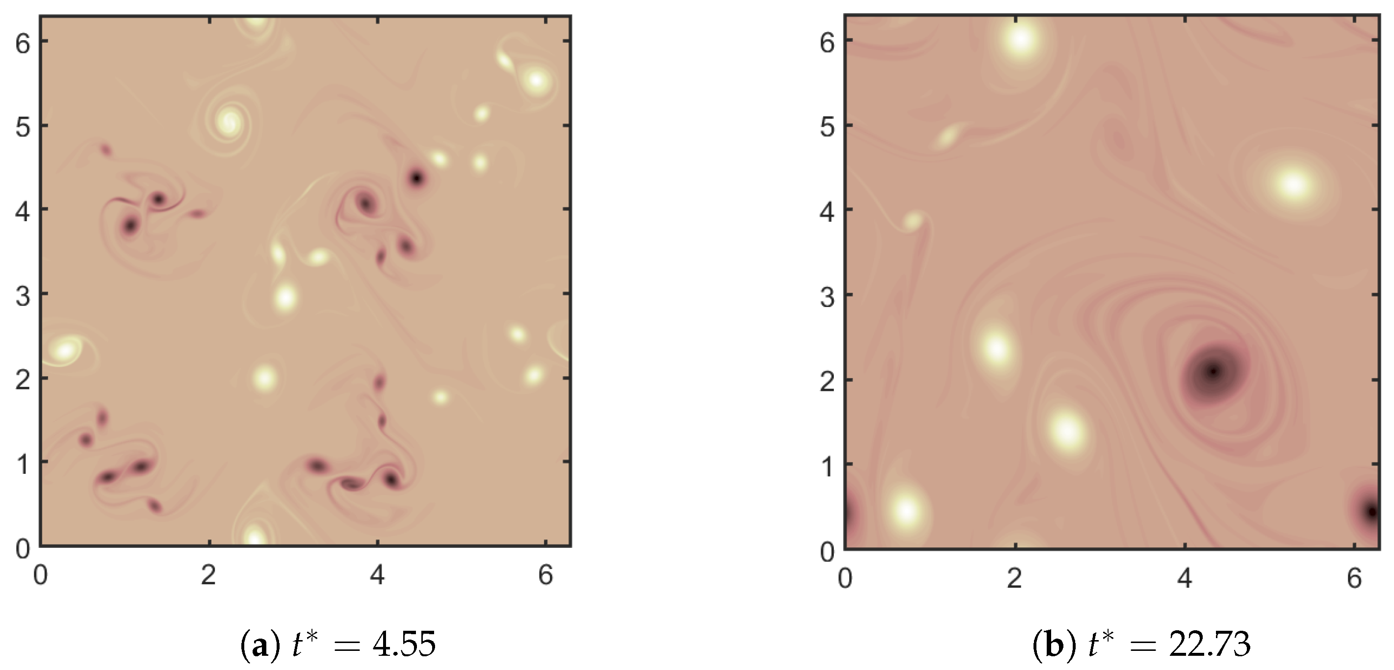
Figure 1. DNS vorticity at nondimensional times t * (scaled by τ L ).
Fluids 07 00154 g001
Figure 2. Filtered vorticity field with filter width Δ = 0.4 at t * = 4.55 .
Fluids 07 00154 g002
Figure 3. Energy spectrum for the DNS field and the filtered DNS field at t * = 4.55 .
Fluids 07 00154 g003
Figure 4. The predicted value of one component of the source term versus the true source terms (plotted in blue dots). The correlation coefficient is shown on the top of the frame. The 45 red line shows a perfect fit.
Fluids 07 00154 g004
Figure 5. The vorticity contours at t * = 11.36 . (a) Filtered DNS vorticity field; (b) LES vorticity field with NN models; (c) Vorticity field on coarse grid with no model.
Fluids 07 00154 g005
Figure 6. The 1D-energy spectrum of the DNS field, the filtered DNS field, the LES field and the coarse grid solution.
Fluids 07 00154 g006
Figure 7. The second-order nondimentional longitudinal structure function D L L * .
Fluids 07 00154 g007
Figure 8. The evolution of the enstropy for the filtered DNS, LES and the under-resolved solution.
Fluids 07 00154 g008
Figure 9. Vorticity contours at t * = 10.42 . (a) Filtered DNS vorticity field; (b) LES vorticity field with NN model; (c) Under-resolved vorticity field on coarse grid.
Fluids 07 00154 g009
Figure 10. The 1D-energy spectrum of the DNS field, the filtered DNS field, the LES field and the coarse grid solution.
Fluids 07 00154 g010
Figure 11. The second-order nondimentional longitudinal structure function D L L * .
Fluids 07 00154 g011
Figure 12. The evolution of the enstropy for the filtered DNS, the LES and the under-resolved solution.
Fluids 07 00154 g012
Publisher’s Note: MDPI stays neutral with regard to jurisdictional claims in published maps and institutional affiliations.