Calculation of the Pressure Field for Turbulent Flow around a Surface-Mounted Cube Using the SIMPLE Algorithm and PIV Data

Abstract

The calculation of the pressure field on and around solid bodies exposed to external flow is of paramount importance to a number of engineering applications. However, conventional pressure measurement techniques are inherently linked to problems principally caused by their point-wise and/or intrusive nature. In the present paper, we attempt to calculate a time-averaged two-dimensional pressure field by integrating PIV (particle image velocimetry) velocity measurements into a CFD code and modifying them by the respective correction step of the SIMPLE algorithm. Boundary conditions are applied from the PIV data as a three-layer area of constant velocities adjacent to the boundaries. A novel characteristic of the approach is the straightforward inclusion of the Reynolds stresses into the source terms of the momentum equations, calculated directly from the PIV statistics. The methodology is applied to three regions of the symmetry plane parallel to the main boundary layer flow past a surface-mounted cube. In spite of findings of deviations from the planar 2D flow assumption, the derived pressure fields and the adjusted velocity fields are found to be reliable, while the intrinsic turbulent nature of the flow is considered without modelling the Reynolds stresses.

1. Introduction

Calculation of the pressure field on and around solid bodies exposed to turbulent flow is an engineering challenge of primary importance to numerous applications, e.g., the calculation of power curves as well as lift and drag coefficients of wind turbines [1], wind loads on structures [2], etc. Although computational fluid dynamics (CFD) does provide a path, the accuracy of the results is heavily dependent on several factors such as the definition of correct boundary conditions and the choice and implementation of the turbulence model, to name but a few. On the other hand, measurements of pressure are almost always of limited spatial discretisation, while area or volume measurements of the velocity field are often available at the lab scale via particle image velocimetry (PIV) technology. The traditional approach in the field of fluid mechanics relies on a simple juxtaposition of CFD and experimental solutions for the purpose of comparison and not on their combination, even though they refer to a common physical problem. One of the concepts of the present study is that of merging different sources of information in order to produce a new, improved solution.

Conventional pressure measurement techniques such as pressure probes of the multiple-hole pitot type or fast-response pressure sensors are either incapable of providing a quantification beyond that of the mean flow field and/or restricted to point-wise or intrusive measurements [3]. Many researchers have proposed experimental methods such as pressure-sensitive paint (PSP) for surface pressure measurements in a wind tunnel [4,5], whereas other researchers used air bubbles to measure static pressures [6]. Nevertheless, these experimental techniques are of restrained applicability, since they are not usually able to capture the whole pressure field in the computational domain.

The PIV (particle image velocimetry) measurement technique constitutes a non-intrusive experimental technique, being able to extract instantaneous velocity fields over the whole domain of interest [7]. Therefore, many scientists have oriented their attention towards the implementation of PIV-based pressure calculation. By utilising instantaneous PIV velocity data and by solving a Poisson pressure equation, instantaneous pressure fields have been extracted for the case of a stationary circular cylinder with $Re=2000$ [8], while the time-averaged pressure field of an annular swirling jet flow has been calculated using stereo-PIV measurements under the assumption of axisymmetric and inviscid flow [9]. The calculation of an instantaneous pressure field for the case of the unsteady wake flow around a cylinder of square cross section by directly solving Navier–Stokes equations and, alternatively, a Poisson pressure equation using stereo-PIV velocity data has also been performed [10]. Various forms of a Poisson pressure equation along with direct solutions of the Navier–Stokes equations were deployed [11] for time-dependent incompressible flows using DPIV (digital particle image velocimetry) velocity data, whilst the surface pressures on a flapping rigid plate utilising data originating from stereo-PIV have also been calculated [12]. Another attempt in the framework of reconstructing pressure from 2D PIV data by solving a Poisson pressure equation [13] deploys Taylor’s hypothesis (TH) for the extraction of an instantaneous pressure field. Eulerian and Lagrangian approaches were adopted by [14] for the determination of instantaneous planar pressure fields from velocity data obtained by the PIV method in turbulent flows, while they also provided guidelines for the PIV temporal and spatial resolution, the PIV interrogation window size and the acquisition frequency. The deployment of various pressure reconstruction methods (including a Eulerian and Taylors’ hypothesis approach), designated for PIV and LPT (Langrangian particle tracking) measurements, was accomplished for a simulated experiment by [15], while ref. [16] assessed a procedure for the extraction of aerodynamic loads and surface pressures on an airfoil for transonic flows using PIV data. Volumetric approaches, where PIV data also include the third component of the velocity as well as some information for its gradient, exist in the bibliography [17,18,19,20].

Although in the aforementioned undertakings, experimental data were utilised for the computation of the respective pressure fields, these were not integrated/assimilated, since the velocity fields remained invariant and no iterative method took place. The idea of integrating measurements into a CFD code is not new, since a methodology appertaining to the family of state observers has been proposed [21], where the SIMPLER algorithm uses partial experimental information as feedback for the reconstruction of the boundary conditions of turbulent flows. State observers can be defined as functions aiming to reconstruct the state of a system from an incomplete set of measurements [22]. The principal motive behind the integration of measurements is the necessity of reproducing the exact structure of real complex flows, especially in disciplines such as meteorology and feedback flow control [23]. The inherent difficulty in calculating adequately real complex flows is directly linked to the uncertainty with regard to the boundary conditions [23]. The creation of a state observer for the integration of three-dimensional PIV velocity measurements into a CFD simulation has recently been accomplished [24].

Another approach aiming at the integration of PIV data and, at the same time, at the reconstruction of the respective pressure field consists of SIMPLE-based methods where the boundary conditions of the velocity are constructed from PIV data. To the authors’ knowledge, only two other attempts following the latter reasoning can be distinguished: ref. [25] extracted pressure fields from two-dimensional PIV snapshots using the SIMPLER algorithm on a non-staggered grid for laminar, incompressible and steady flow, whereas ref. [26] computed pressure from two-dimensional PIV data for incompressible, laminar steady and unsteady flows. Therefore, the novelty characterising the present research is its application to a turbulent flow with direct computation of Reynolds stresses from the PIV statistics and their inclusion in the source terms of the Reynolds-averaged Navier–Stokes (RANS) equations. The utilisation of a turbulence model can also be avoided through the implementation of direct numerical simulation (DNS) [27], but DNS is not always feasible, as extensive computational resources are usually required.

All the aforementioned methods for measurement integration into CFD codes do not take into account the uncertainty of the measurements or the CFD solution, so the way that experimental and computational resources are combined is not always mathematically rigorous and problem-independent. For these reasons, many researchers found the strict mathematical framework of data assimilation (DA) methods appealing, where the uncertainty of the discrete sources of information is modelled by the respective error covariance matrices. DA methods have been used widely in the discipline of weather forecasting and earth sciences [28,29,30] for years, and their utilisation is expanding rapidly in different scientific fields. Data assimilation can be defined as an approach/method for combining observations with model output with the objective of improving the latter [31]. Concerning these DA methods (where the uncertainty is quantified), variational data assimilation and adjoint-based optimisation has been performed [32] using PIV data collected from a wind tunnel as well as synthetic measurements to generate inflow conditions for direct numerical simulations (DNS). The combination of PTV (particle tracking velocimetry) and DNS for the analysis of vortical motion in the shear layers of a jet by implementing a reduced-order Kalman filter (KF) has been presented [33], whereas the ensemble Kalman filter has also been used [34] for the combination of pressure measurements acquired through experiments in a wind tunnel with a CFD code for the case of a square cylinder. The DA approach is not the same as the data integration presented here as, in DA, the two sources of information remain invariant as they are combined to form a new output. This relies on rigorous calculations to quantify the uncertainty in both sources. Although there are several robust approaches to this, which lead to an overall reduction in uncertainty, none are based on the preservation of the conservation laws inherent in the fluid dynamics equations. We have found that integration of data into a CFD solution procedure has not received significant attention, and this has been the starting point for the first steps in the present research.

Here, two-dimensional PIV velocity data [35] for the turbulent flow past a surface mounted cube are integrated into a CFD code based on the SIMPLE algorithm. Turbulence is included in the Reynolds-averaged Navier–Stokes equations through the Reynolds stresses, avoiding the need for a turbulence model as they are computed directly using the statistics of the PIV experiment. To the authors’ knowledge, this is the first time this has appeared in the literature, and the combination with the SIMPLE pressure correction methodology serves the ultimate goal of calculating the respective pressure field through simultaneous adjustment of the velocity fields in order to satisfy the conservation of mass and momentum. The structure of this paper is as follows: in Section 2, an extended analysis of the methodology and its necessary components is presented. In Section 3, the respective results of the estimates of pressure and velocities for three planes around the cube are illustrated, and a synopsis with conclusions is given in Section 4.

2. Computational Method

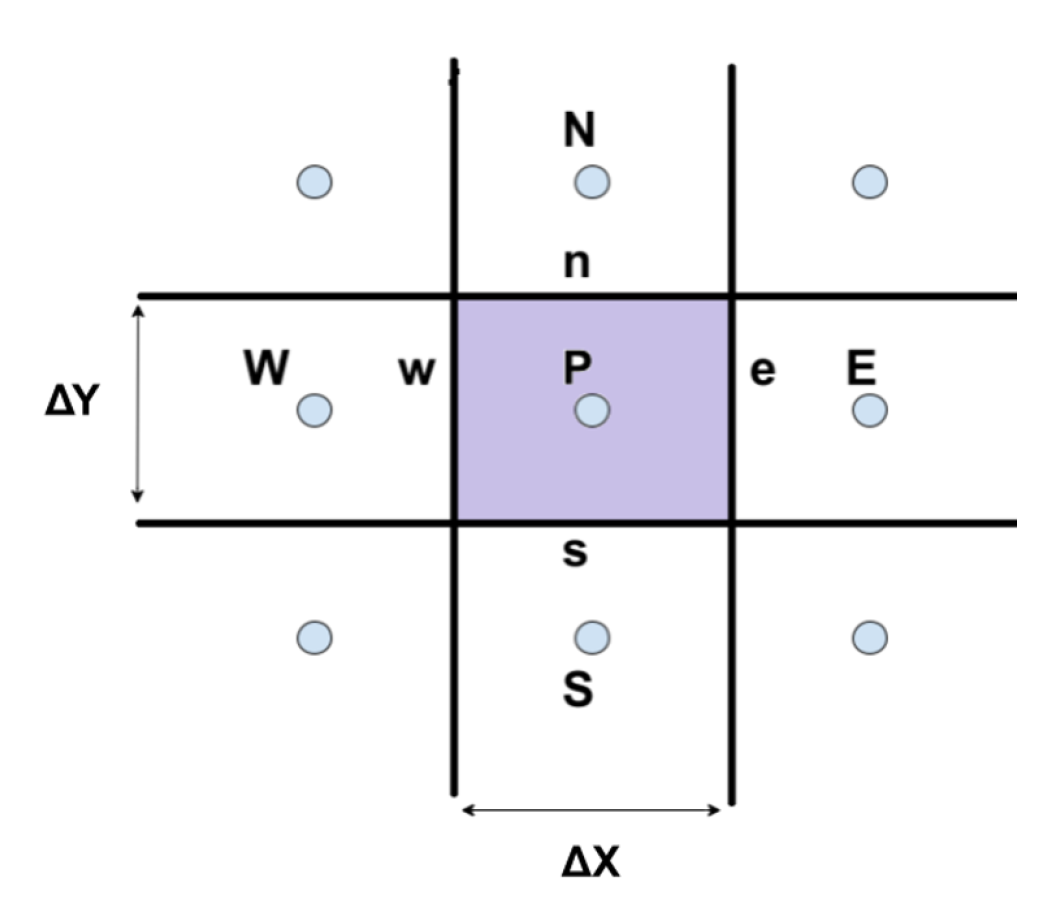
2.1. Basic Equations and Discretisation

An in-house code has been used for the implementation of the present methodology. The code has been used in various forms and extensions over the years [36,37] and is a standard finite volume implementation of the SIMPLE algorithm on a Cartesian grid with collocated variables. A brief description of the code follows. The basic equations that are solved and participate in the iterative method are the steady state Reynolds-averaged Navier–Stokes (RANS) equations in two dimensions i.e., Equation (1), along with the continuity equation i.e., Equation (2), for incompressible flow.

$$\rho {\overline{u}}_j\frac{\partial {\overline{u}}_i}{\partial x_j}=\frac{\partial \overline{p}}{\partial x_i}+\mu \Delta {\overline{u}}_i-\rho \left(\frac{\partial \overline{u_i^{\prime }{u}_j^{\prime }}}{\partial x_j}\right)$$

(1)

$$\nabla u=0$$

(2)

where the overbar denotes Reynolds-averaged quantities, $i,j=1$ or 2 (with respect to x and y directions), $\Delta$ is the Laplace operator, $\rho$ and $\mu$ are the density and dynamic viscosity, respectively. The last term on the right-hand side of Equation (1) corresponds to the Reynolds stresses. It is noted that from now on, the time-averaged velocity components with respect to the x and y directions are indicated u and v, respectively (without overbar), unless denoted differently. It has to be denoted that although the continuity equation is not solved directly, it constitutes a basic element of the SIMPLE pressure correction algorithm [38] and will also be used as a measure of quality quantification of the initial PIV data.

By implementing the finite volume method in Equation (1), a pentadiagonal system is derived shown in Equation (3), where $\Phi$ is equal to the velocity component with respect to the x or y direction (i.e., u or v, respectively), ${\alpha }_{P/S/E/N/W}$ are constant coefficients depending on the geometry and the deployed discretisation schemes, and $S_P^{\Phi },S_U^{\Phi }$ are source terms. A clarification of the indices $P, S, E,N$ and W is better illustrated in Figure 1, where a typical finite volume of this problem is shown (the depth, z, is considered equal to unity as a two-dimensional problem is confronted). P stands for the cell centre where the equations are solved, while $S, E, N$ and W correspond to South, East, North and West.

$$({\alpha }_P^{\Phi }-S_P^{\Phi }){\Phi }_P={\alpha }_N^{\Phi }{\Phi }_N+{\alpha }_S^{\Phi }{\Phi }_S+{\alpha }_E^{\Phi }{\Phi }_E+{\alpha }_W^{\Phi }{\Phi }_W+S_U^{\Phi }$$

(3)

For the discretisation of the convective terms, the hybrid differencing scheme was implemented, while for the diffusive terms, a central differencing scheme was applied.

The pressure gradient in Equation (1) is contained in the source term $S_U^{\Phi }$ of Equation (3) and discretised using the central differencing scheme. All variables (i.e., $P, u$ and v) are stored at the centre of every cell/finite volume (collocated approach), and a corresponding modification [39] is implemented to avoid checkerboard pressure oscillations. For the present application, the distance between the cell centres is constant (uniform grid), and the computational grid is chosen to be almost identical to the PIV method (see [40,41]). The slight difference between the PIV and computational grid is presented in the next section.

The aforementioned choice is based on the reasoning that a disadvantage of the PIV method in comparison to a CFD solution is its low spatial resolution. Thus, the choice of an almost identical CFD grid to PIV came as the most natural selection, since the experimental information was available only on the PIV nodes. Although remapping information onto a denser grid is an obvious option, here, we chose to keep things simple in order to better assess the effect of individual parameters and to test the method in the least computationally intensive way.

In the standard implementation of the code, several eddy viscosity-type turbulence models are available [42,43], while previous applications included LES [44]. Here, a novel approach is adopted whereby the Reynolds stress terms, after the implementation of finite volume method and linear interpolation on the faces of each cell (i.e., $n, s, w$ and e), are included in the source terms of Equation (3) in discretised form (for the x and y direction, respectively):

$$-[{\left(\rho \overline{{u^{\prime }}^2}\delta y\right)}_e-{\left(\rho \overline{{u^{\prime }}^2}\delta y\right)}_w]-[{\left(\rho \overline{u^{\prime }{v}^{\prime }}\delta x\right)}_n-{\left(\rho \overline{u^{\prime }{v}^{\prime }}\delta x\right)}_s]$$

(4)

$$-[{\left(\rho \overline{u^{\prime }{v}^{\prime }}\delta y\right)}_e-{\left(\rho \overline{u^{\prime }{v}^{\prime }}\delta y\right)}_w]-[{\left(\rho \overline{{v^{\prime }}^2}\delta x\right)}_n-{\left(\rho \overline{{v^{\prime }}^2}\delta x\right)}_s]$$

(5)

If the number of acquired PIV snapshots is N, then Reynolds stresses can be calculated using the velocity statistics and can be added to the source terms of the momentum equations, while their values remain constant throughout the iterative method (see Section 2.2):

$$\overline{u_i^{\prime }{u}_j^{\prime }}=\sum _{k=1}^N\frac{u_{k,i}^{\prime }{u}_{k,j}^{\prime }}{N}$$

(6)

where generally, $u_i^{\prime }=u_i-\overline{u_i}$ and $i=1$ or 2 with respect to the x or y direction ($u_i$ corresponds to an instantaneous velocity in this context). This approach is an alternative to the implementation of a turbulence model, assuming that the turbulence model would introduce greater uncertainty than the PIV data.

The classic formulation of the SIMPLE algorithm includes a pressure correction equation which is derived from the continuity equation combined with correction equations for velocity as well as pressure. By implementing finite volumes and suitable discretisation schemes, the following equation is derived [38]:

$${\alpha }_P^{P^{\prime }}{P}_P^{\prime }={\alpha }_N^{P^{\prime }}{P}_N^{\prime }+{\alpha }_S^{P^{\prime }}{P}_S^{\prime }+{\alpha }_E^{P^{\prime }}{P}_E^{\prime }+{\alpha }_W^{P^{\prime }}{P}_W^{\prime }+S_U^{P^{\prime }}$$

(7)

In Equation (7), $P^{\prime }$ is the pressure correction, equal to the difference between the current pressure value and the last iteration, ${\alpha }_{P/S/W/N/E}^{P^{\prime }}$ are coefficients with dependence on the coefficients of Equation (3), the discretisation schemes and the geometry, and $S_U^{P^{\prime }}$ is a source term. The source term is basically equal to the residual of the continuity equation of every iteration for the finite volume with cell centre P, and for that reason, the initial PIV data continuity residual is of vital importance for the convergence of the iterative method.

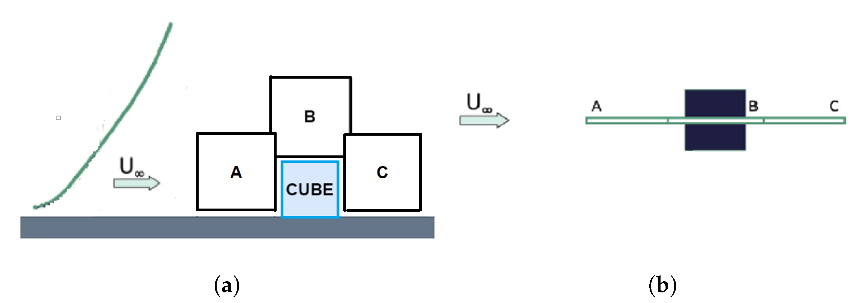
2.2. Geometry and Experimental Configuration

The geometry and the configuration of the experiment [35] on which the method is applied are given in Figure 2.

From the results illustrated in [35], the present method is applied to the case of high shear flow around a solid, surface-mounted cube and for the planes that lay on the flow’s symmetry plane (planes A, B and C), being parallel to the vector of the free stream velocity, in order to satisfy the 2D flow assumption.

The coordinates X and Y in all the forthcoming figures are non-dimensionalised with the height of the cube, $H_c=0.11$ m, whilst the thick black line represents the boundary of the cube. It has to be clarified that the distance of planes A, B and C from every solid boundary (i.e., walls of the cube and ground) is close to 1 cm, to ensure optical access during the PIV experiment [35]. The working fluid is air with density $\rho =1.21$ kg/m${}^3$ and dynamic viscosity $\mu =17.9\times {10}^{-6}$ kg/(m·s). The Reynolds number at cube height exceeded $2\times {10}^4$ throughout the realisation of the experiment; namely, it was over the suggested limit for Reynolds number independence in wind tunnel tests on buildings [35].

Apart from the PIV experiment, pressure taps on the walls of the cube were utilised for the extraction of profiles of the pressure coefficient, $C_{P_{EXP}}$. The pressure measurements were performed along the plane of symmetry on the front, the roof and the back face, which is perpendicular to the velocity vector of the free stream, as can be observed in Figure 3 [45]. The maximum experimental error of the pressure coefficient is derived equal to $4.5\%$ with error propagation, owing to the fact that the maximum measurement errors of the pressure and the reference velocity are $3\%$ [35] and $1.67\%$, respectively.

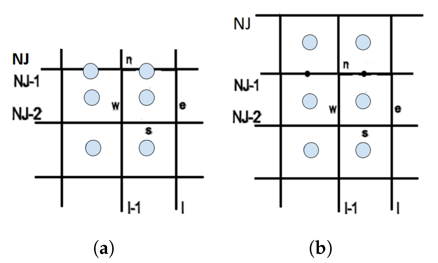
2.3. Boundary Conditions and Iterative Method

Initial attempts to use Dirichlet boundary conditions (i.e., constant velocities, u and v, and constant convective terms) were ineffective, and a new type of boundary conditions (BC) is imposed in the present research, which requires a three-layer area (e.g., the area defined by the grid cells below lines $NJ$, $NJ-2$, $NJ-1$ in Figure 4a; note that “cell” NJ is a zero area cell defining the boundary) where constant velocities u and v are imposed, corresponding to constant first and second normal derivatives. These velocities are equal to those originating from the PIV method without any change, except for those on the grid lines defining the boundaries, where a linear interpolation takes place. The experimental and computational grids are slightly different on the boundaries, since the finite volume of the boundary for the PIV grid (Figure 4b) is not of zero area as for the CFD one (e.g., for the finite volume/grid line $NJ$ in Figure 4a). For example, on the northern grid line, $NJ$, the velocities are given by the equation $\Phi {\left(NJ\right)}_{CFD}=(\Phi {(I,NJ)}_{PIV}+\Phi {(I,NJ-1)}_{PIV})/2$, where $\Phi =u$ or v. The index $PIV$ denotes that the velocities emanate directly from the experimental data (i.e., PIV grid), while the index $CFD$ corresponds to the velocity utilised for the computational procedure (i.e., CFD grid). The former reasoning is applied for every boundary of the domain. Regarding the boundary conditions of the pressure correction equation, Neumann BC are imposed on the internal boundaries of the three-layer area, while for the cells within this area, the pressure correction equation is not solved.

For the commencement of the iterative procedure, the initial guess of the values of the velocities are those of the PIV method, while the initial pressure field is set to zero. The pressure is calculated with respect to a reference value, chosen at a specific point where the flow could be considered the least disturbed. This is a point to which further attention will be directed in the next sections. A field of Reynolds stresses, computed directly from the PIV data, is also included in the source terms of the pentadiagonal system of equations (Equations (3)–(5)) and remains constant throughout the iterative method. The system is solved with the alternating direction implicit method (ADI).

The iterative algorithm is composed of the following steps:

• The pressure correction equation, i.e., Equation (7), is solved once having introduced as initial velocity fields those emanating from the PIV measurements;
• The velocity and pressure fields are corrected by implementing the SIMPLE pressure correction steps [38], including the Rhie and Chow corrections [39];
• The RANS momentum equations are solved with the corrected velocity and pressure fields, having included the Reynolds Stresses from the PIV data. Reynolds stresses are not corrected in this work.
• The aforementioned iterative steps are repeated until there is the best possible convergence.

Overall, for application of the present methodology, the in-house code was adjusted in order to: (a) receive PIV data as input (initial fields), (b) include the PIV-calculated Reynolds stresses in the source terms of Equation (3) and (c) impose the above-mentioned customised boundary conditions.

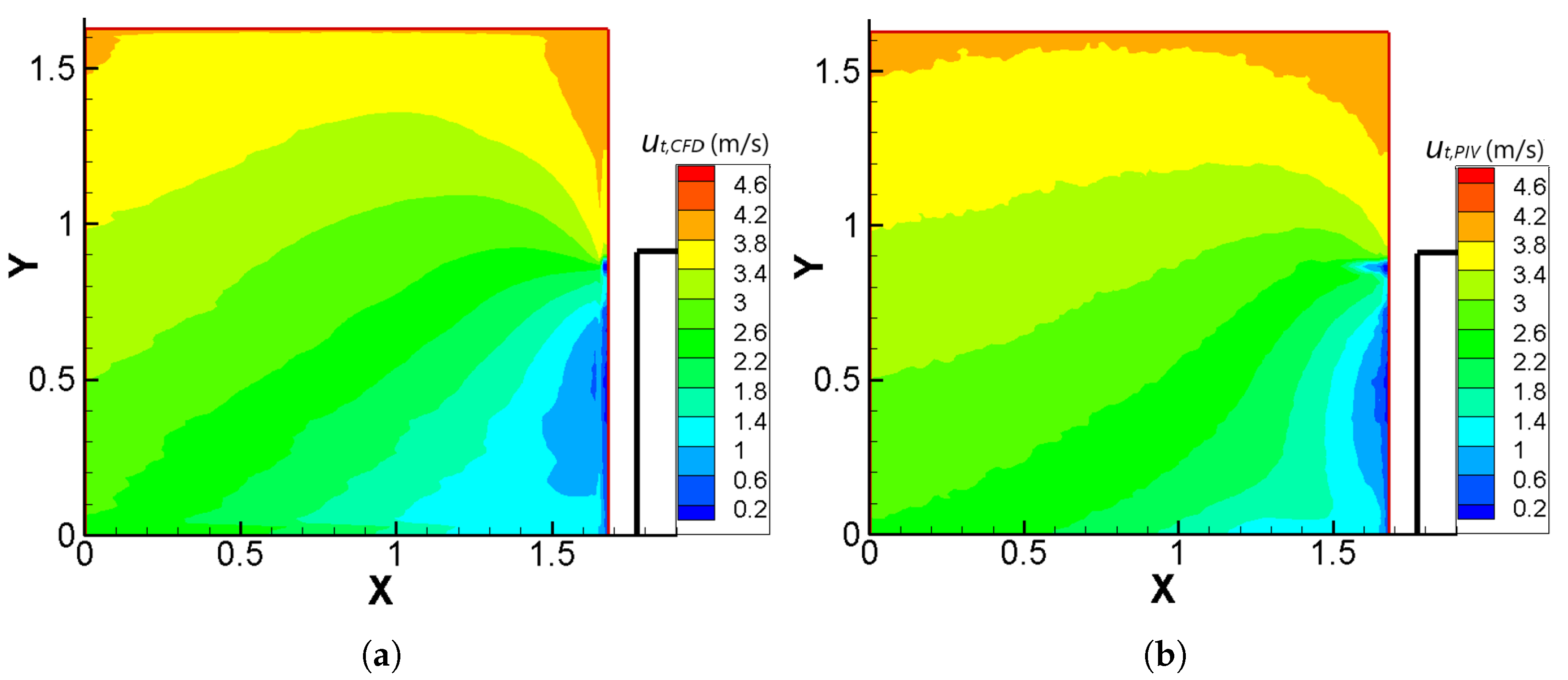
2.4. Post-Processing Tools and Validation

For the validation of the initial PIV data as well as for the final solution, a number of criteria have been used. Firstly, the initial continuity residual is calculated, as follows:

$$\frac{u_E-u_W}{2\Delta x}+\frac{v_N-v_S}{2\Delta y}=CR$$

(8)

where $E, W, N$ and S stand for the eastern, western, northern and southern cell centre and $CR$ is the continuity residual. The above-mentioned equation is evaluated on the cell centre P (see Figure 1) and is applied directly to the PIV data under the following non-dimensional form:

$$CRN=\frac{CR}{\left(\frac{<u_{t,PIV}>}{2\Delta x}\right)}$$

(9)

with:

$$<u_{t,PIV}>=\sum _{k=1}^{NI·NJ}\frac{{\left(\sqrt{u_{PIV}^2+v_{PIV}^2}\right)}_k}{NI·NJ}$$

(10)

where <$u_{t,PIV}$> is the spatially and time-averaged value of the total velocity of the PIV velocity field.

The integral form of the continuity equation is also evaluated for the whole domain of the examined PIV data, yielding a characteristic value that represents the residual of mass inside the whole experimental domain:

$$ICR=\left({\int }_{Y_{min}}^{Y_{max}}\rho u_{E}dy-{\int }_{Y_{min}}^{Y_{max}}\rho u_{W}dy\right)+\left({\int }_{X_{min}}^{X_{max}}\rho v_{N}dx-{\int }_{X_{min}}^{X_{max}}\rho v_{S}dx\right)$$

(11)

where indices $max$ and $min$ indicate the maximum and minimum dimensions of the experimental domain, and the velocities participating in the integrals are those which are normal to the boundaries of the PIV domain. In an analogy to CR, the $ICR$ (integral continuity residual) is non-dimensionalised.

$$ICRN=\frac{ICR}{\rho <u_{t,PIV}>(X_{tot}+Y_{tot})/2}$$

(12)

with $X_{tot}=X_{max}-X_{min}$, $Y_{tot}=Y_{max}-Y_{min}$ and $<u_{t,PIV}>$ as defined in Equation (10). Similar to the denominator in the expression for the $CRN$, the denominator in Equation (12) constitutes a characteristic mass flux of the PIV velocity field. The integrals in Equation (11) are numerically calculated by applying the Simpson 1/3 method [46].

The residuals $ICRN$ and $CRN$ constitute an indication of the uncertainty in the experimental data and, in the present case, of the extent that the assumption of two-dimensionality of the flow is accurate. This emanates from the fact that the third velocity component has been ignored in their calculation, based on the choice of measurement planes lying on the flow’s symmetry plane. Hence, a part of these residuals can be attributed to the possible 3D structures of the flow, especially near solid boundaries.

A deployed measure of validation of the CFD solution is the difference/error between the CFD local velocity estimate and that acquired directly through the PIV measurements, shown in Equation (13), in order to quantify the level of velocity correction which takes place throughout the iterative method.

$${ϵ}_{corr,u_t}(\%)=100·\frac{|u_{t,CFD}-u_{t,PIV}|}{|<u_{t,PIV}>|}$$

(13)

where subscripts $PIV$ and $CFD$ correspond to the PIV velocities and the CFD velocity estimate, respectively, $u_t$ is the total velocity and <$u_{t,PIV}$> is as defined in (10). The velocities $u_{t,PIV}$ and $u_{t,CFD}$ are local velocities, defined in every cell centre. The denominator is chosen to be <$u_{t,PIV}$> instead of the local velocity e.g., $u_{t,PIV}$, to avoid possible fictitious overestimation in regions of small total velocities.

3. Results and Discussion

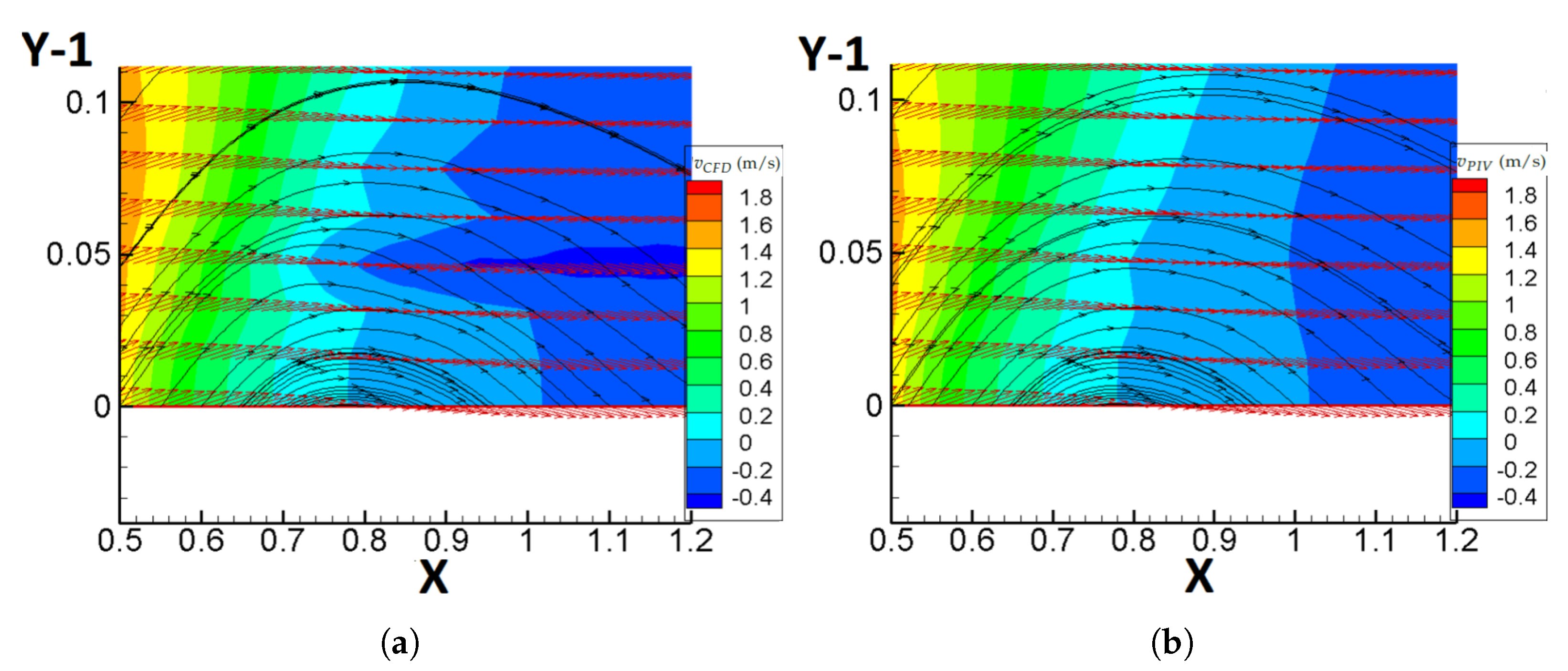
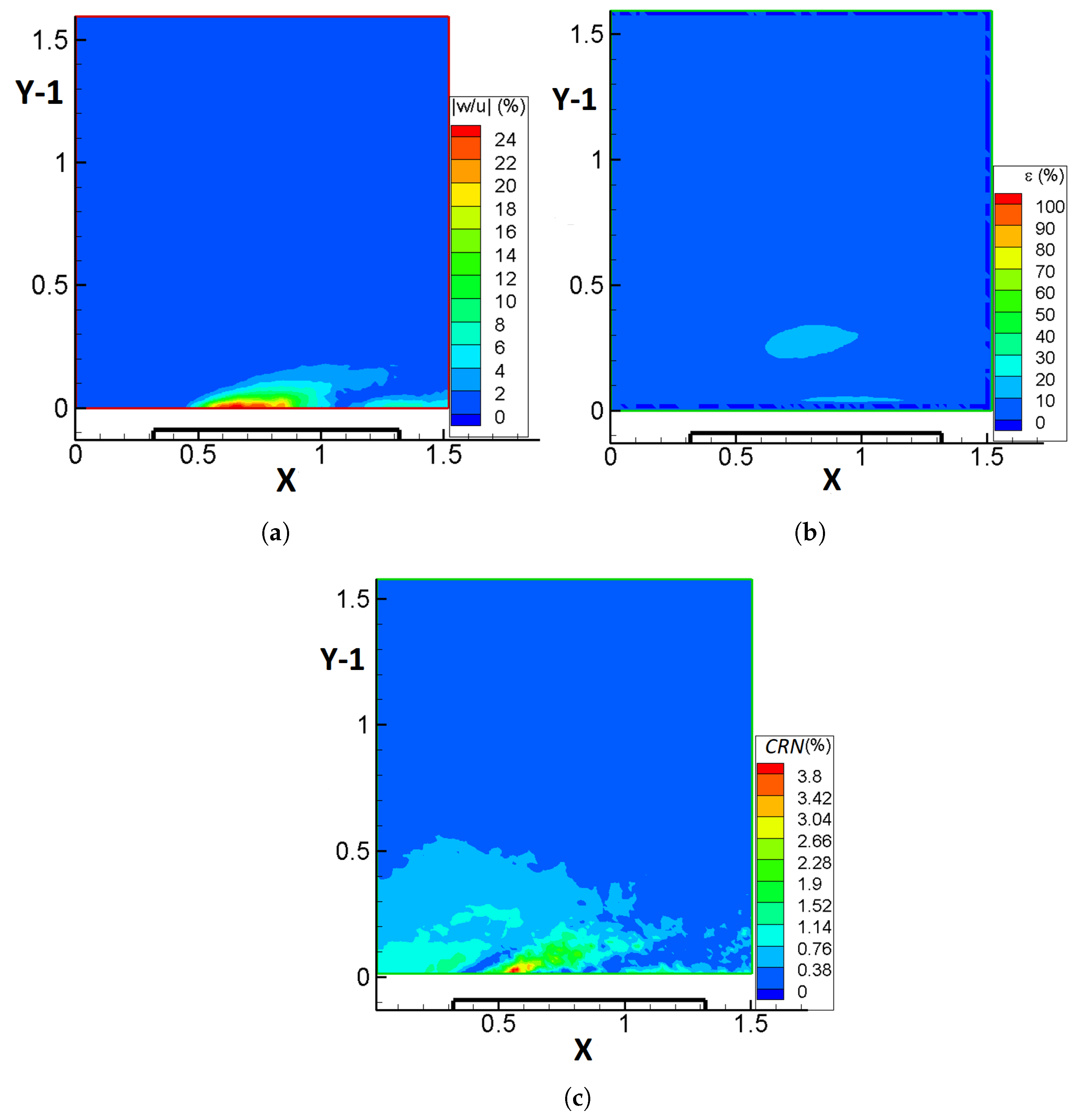
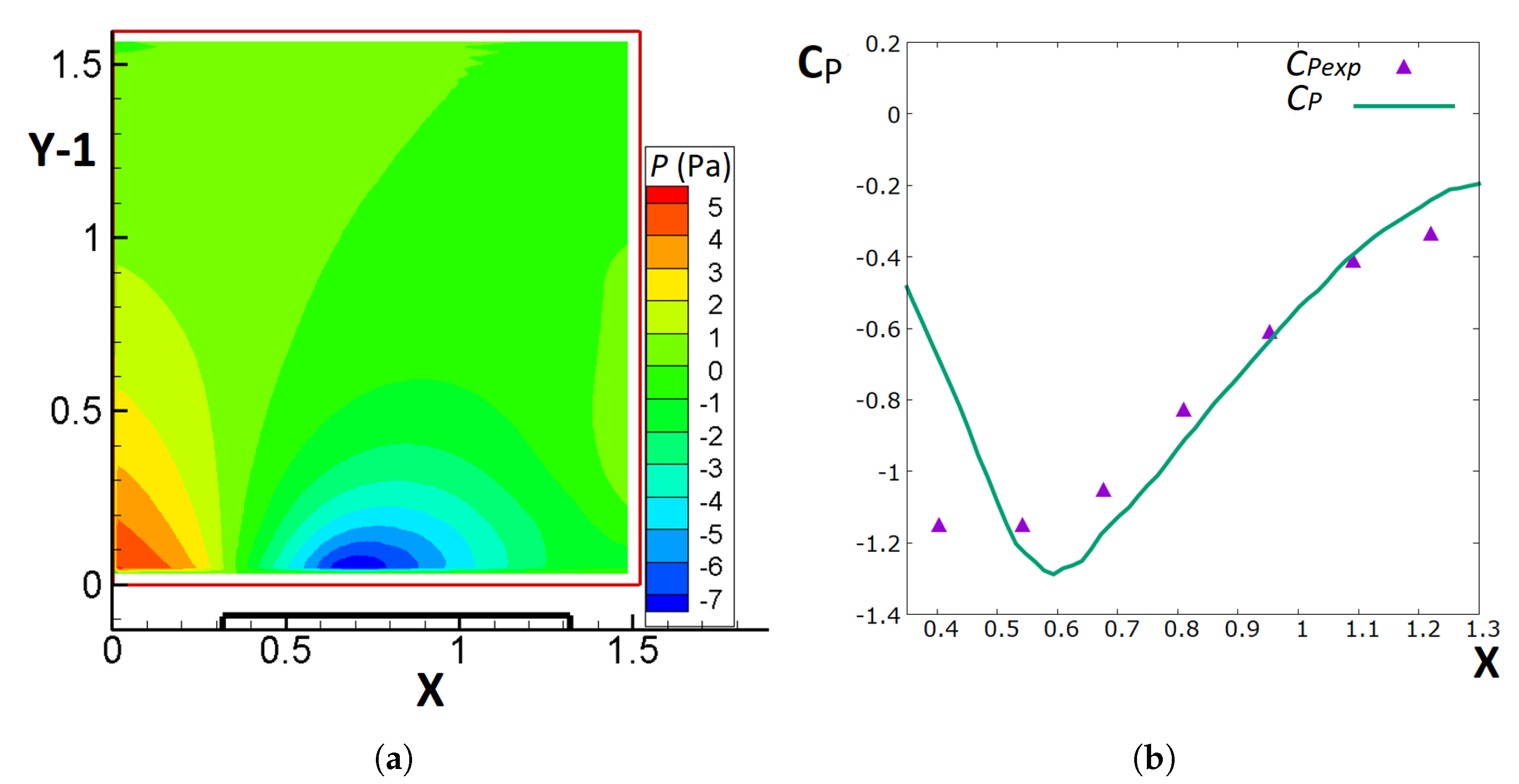
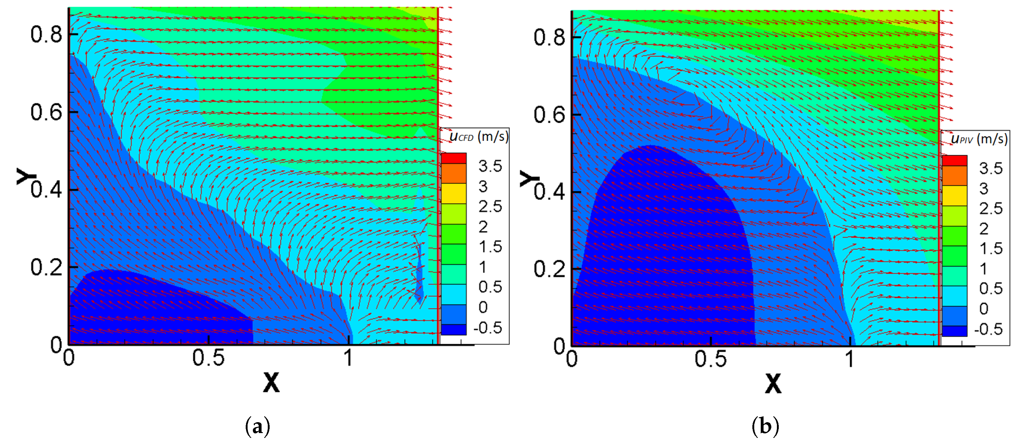
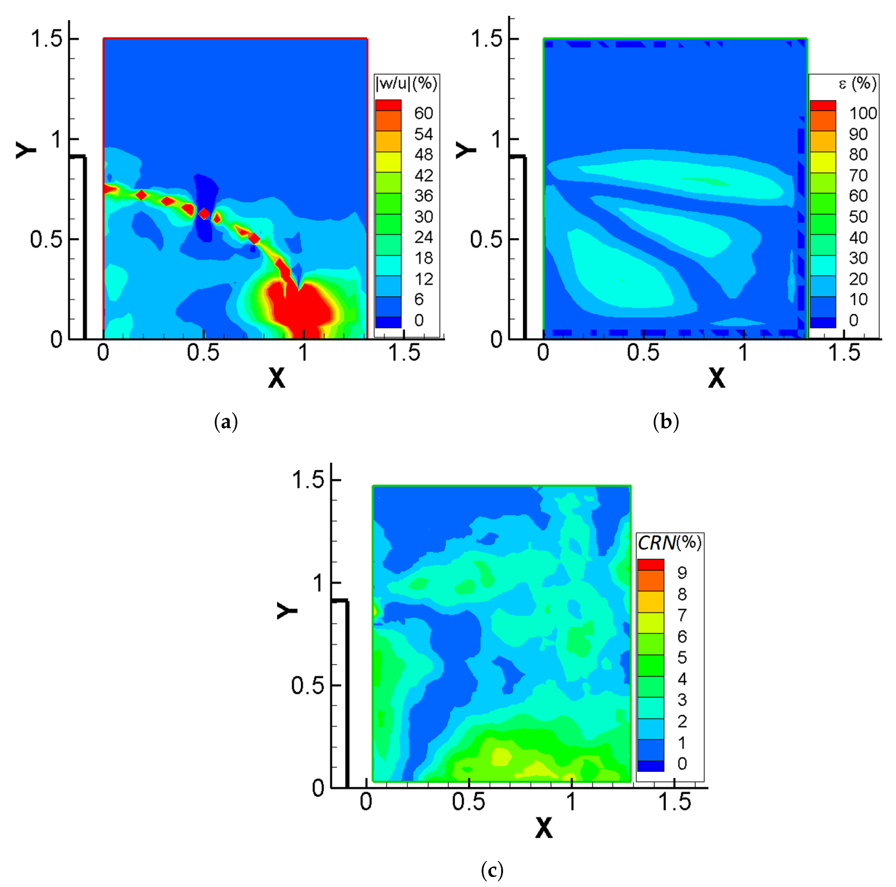
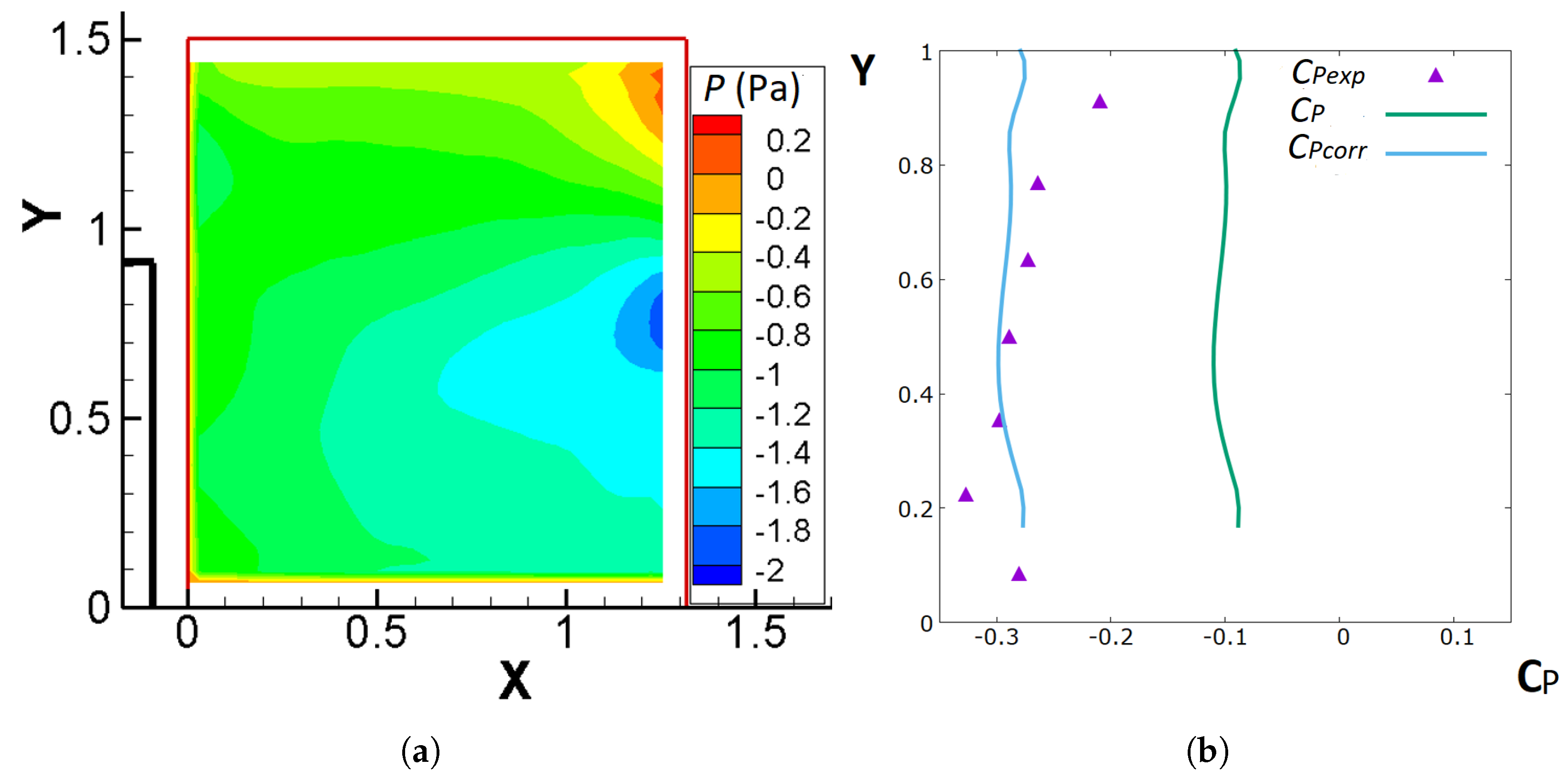
3.1. Results for Plane A

The basic geometric and grid parameters for both the PIV measurements and the CFD calculations are shown in tabulated form in

Table 1. Basic geometric and grid parameters: $NI$ and $NJ$ are the numbers of the grid lines with respect to the x and y direction, while $X_{tot}$ and $Y_{tot}$ are the x and y dimensions of the computational domain.

Plane	$\mathit{N}\mathit{I}$	$\mathit{N}\mathit{J}$	${\mathit{X}}_{\mathit{t}\mathit{o}\mathit{t}}/{\mathit{H}}_{\mathit{c}}$	${\mathit{Y}}_{\mathit{t}\mathit{o}\mathit{t}}/{\mathit{H}}_{\mathit{c}}$
A	130	126	1.68	1.63

. Owing to the fact that the south boundary ($Y=0$) of plane A has a non-dimensional distance of $0.09$ from the ground/base of the cube, the top upstream corner of the cube is located at a non-dimensional height of $Y=0.91$ and not $Y=1$ in all the forthcoming figures.

The contours of the total velocity, $u_{t,CFD}$, calculated with the above-mentioned CFD methodology are shown in Figure 5a, whilst in Figure 5b those of the uncorrected PIV total velocity, $u_{t,PIV}$ are given.

As expected, the CFD estimate closely resembles the initial PIV data. The position of the stagnation point, i.e., approximately $(X_{max},0.7)$, and the range of the velocity values is invariant after the iterative method. The aforementioned arguments are further supported by Figure 6b, where the error, as expressed in Equation (13), is presented. More specifically, only in the area adjacent to the boundary of the cube and especially near its top upstream corner where the flow accelerates does the error appear to reach its maximum value. The CFD calculation fails to adequately represent the physics of the flow in this area, most probably due to the poor spatial resolution. However, the error value far from the cube tends to zero.

The greater difference between CFD calculations and PIV data near the cube may also be attributed to the appearance of 3D flow structures near the upstream wall. This qualitative statement is quantified in Figure 6a, where the absolute value of the ratio of the third velocity component w, acquired through stereo-PIV, over the u velocity component, is given in the form of contours. As can be observed, in the area near the cube, w takes values comparable to those of the u velocity component, justifying at least part of the discrepancy between the CFD velocity estimate and the PIV data.

A direct consequence, originating from the 3D structure of the flow near the cube, is the increase of the continuity residual (represented by the $CRN$ and $ICRN$), since the third velocity component and its gradient are not taken into account. As can be seen in Figure 6c, $CRN$ reaches the highest values (about 30–40%) near the upstream wall of the cube. Thus, the quantities $|w/u|$ and $CRN$ are closely related and play a significant role in the success of the presented method. From the integral expression of the continuity equation, $ICRN$ is equal to $-62\%$. This high percentage can mainly be attributed to the way that $ICRN$ is normalised in Equation (12). The value itself cannot reveal much, but it is going to be compared with the value corresponding to the experiment on plane B and C.

In general, because of the 2D assumption of the plane of symmetry, the lower the level of $|w/u|$, the lower the value of $CRN$ and $ICRN$, leading to better convergence, more reliable results and lesser discrepancy between the CFD and PIV velocities. However, it should be noted that a zero PIV continuity residual does not ensure perfect implementation of the method, since several factors can deteriorate the situation, such as the temporal resolution of the PIV experiments (a critical parameter for the quality of the statistics of the PIV data), the spatial CFD and PIV resolution, as well as other numerical errors.

Figure 7a shows the contours of the relative pressure on plane A with respect to a reference pressure taken at a point near the top upstream corner of plane A, where the flow approaches free stream conditions. Figure 7b constitutes a comparative diagram between the extracted CFD estimate of the profile of the pressure coefficient, $C_P$ and the measurements (i.e., $C_{P_{exp}}$ [45]). From the calculated pressure fields, the profile of the pressure coefficient $C_P$, computed by Equation (14), is extracted near the walls of the cube (at a distance of approximately 1 cm, which was the minimum distance of PIV measurements from the wall). The Y-axis in Figure 7b corresponds to the non-dimensional distance from the south boundary of the domain ($Y=0.91$ denotes the upper edge of the cube).

$$C_P=(P-P_{ref})/\left(P_{dyn}\right)$$

(14)

where $P_{ref}=0$, $P_{dyn}=1/2\rho U^2=5.99$ Pa and U is the free stream velocity.

The pressure contours, shown in Figure 7a, present a reasonable behaviour, since the maximum value is observed in the area adjacent to the stagnation point and is also in agreement with Figure 5 (i.e., $(X_{max},0.7)$). Near the corner, there is a pressure drop due to flow acceleration. In the region adjacent to the western (inlet) and the northern boundary, the (relative) pressure is equal to zero, since the flow demonstrates free-stream behaviour.

Regarding the comparison between $C_{P_{exp}}$ and $C_P$, it is marked that there is a slight difference between them (i.e., the maximum difference is about $10\%$ of $C_{P_{exp}}$), which is probably caused by: (a) the reference pressure not being exactly the same as the experimental reference pressure, which was outside the experimental domain available here and (b) numerical and experimental errors.

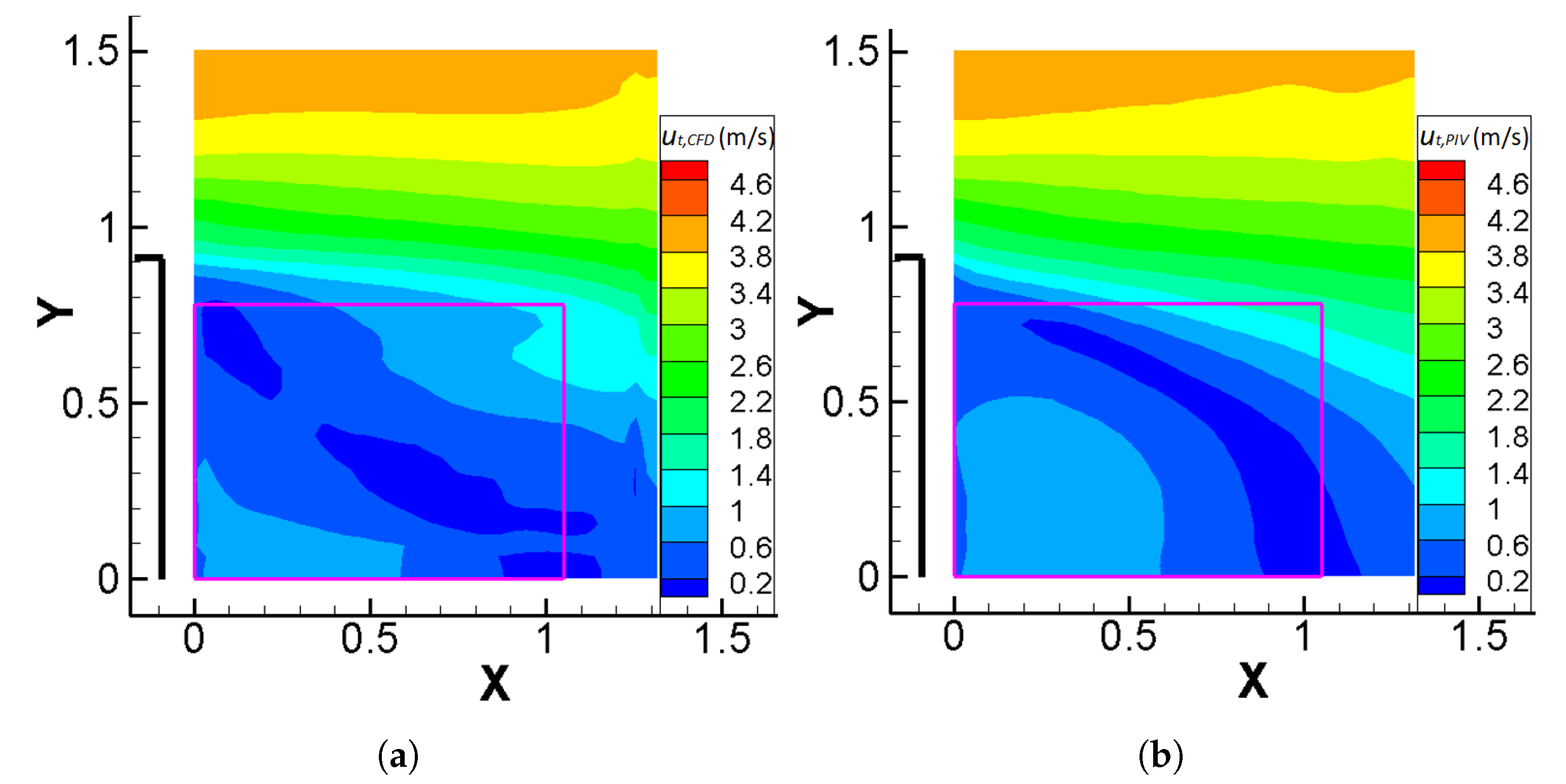
3.2. Results for Plane B

As for plane A, in

Table 2. Basic geometric and grid parameters: $NI$ and $NJ$ are the numbers of the grid lines with respect to the x and y direction, while $X_{tot}$ and $Y_{tot}$ are the x and y dimensions of the computational domain.

Plane	$\mathit{N}\mathit{I}$	$\mathit{N}\mathit{J}$	${\mathit{X}}_{\mathit{t}\mathit{o}\mathit{t}}/{\mathit{H}}_{\mathit{c}}$	${\mathit{Y}}_{\mathit{t}\mathit{o}\mathit{t}}/{\mathit{H}}_{\mathit{c}}$
B	99	104	1.52	1.60

, the basic geometric and grid parameters for the case of plane B are given. These parameters are kept constant for the CFD calculations.

The contours of the CFD estimate of the total velocity, $u_{t,CFD}$, as well as those of the PIV total velocity, $u_{t,PIV}$, are displayed in Figure 8a,b, respectively.

Similar to the behaviour observed for plane A, the discrepancy between the two solutions caused by the correction of velocities through the pressure correction algorithm is not significant. The form and the shape of the region of low velocities (blue region) is preserved in the CFD total velocity field and the range of the velocities is almost the same for both figures. For both solutions, the flow accelerates close to the upstream corner of the cube.

Figure 9 shows contours of the v velocity component, extracted by the CFD calculation (Figure 9a), as well as those originating from the PIV data (Figure 9b). It is interesting to note the indication of a recirculation zone in the above-mentioned area of low total velocities, which is marked by the positive values near the upstream boundary and the negative values near the downstream boundary and appears similar for both the PIV data and the CFD calculation. This is supported by Figure 10, where the vectorial fields and streamlines of the PIV and CFD total velocity along with contours of v are given for an area near the south boundary (indicated by the pink box in Figure 9), since a clear change of direction, tending to 180 degrees, is observed for the velocity vector. This recirculation region probably extends outside the computational domain, near the solid boundary of the cube.

Figure 11b illustrates that the error/difference between the two velocity fields is kept under 10–20%. The maximum value of $20\%$ is observed in a very limited area and for the rest of the computational domain, the difference is below $10\%$. Hence, the discrepancy between the two velocity fields for plane B, is markedly lower than that derived for plane A. The lower value of the difference can partially be attributed to the significantly lower continuity residual, $CRN$. Figure 11c shows that the values of $CRN$ are below $4\%$, namely the maximum value of this quantity for plane B is ten times lower than than that for plane A.

A more detailed analysis of Figure 11c indicates that near the boundary of the cube, the continuity residual increases, which is in accordance with the conclusion already extracted for plane A. By juxtaposing Figure 8 and Figure 11c, it can be concluded that the maximum value of $CRN\%$ is obtained at the commencement of the area of low total velocities. Figure 11a, confirms that in this area, the third velocity component, w, becomes significant in comparison with the u velocity component. The latter observation further confirms the existence of a correlation between the continuity residual and the relative magnitude of the third velocity component i.e., the assumption of two-dimensionality of the flow.

The contours of pressure as well as a comparative diagram between the experimental and the CFD-estimated profiles of the pressure coefficient on the wall of the cube are given in Figure 12a,b respectively. The X-axis in Figure 12b corresponds to the non-dimensional distance from the upstream boundary of the domain (the roof of the cube is between $X=0.3$ and $X=1.3$). The position of the reference pressure is located on the upper left corner of the computational domain, assuming that the flow there is almost free-stream and, therefore, the discrepancy between the experimental reference and the CFD one is minimised (the experimental reference point was located outside the boundary layer of the wind tunnel).

By consulting both figures, it can be contended that the results are physically consistent. Near the upstream boundary of the PIV plane, positive pressure values are observed, affected by the stagnation region on the upstream face of the cube, whilst near the roof of the cube, negative pressure values are acquired, which is in line with observations of other researchers [47,48].

Figure 12b reveals that there is a slight difference between the experimental [45] and CFD-estimated $C_P$ profiles, which can be attributed to the following reasons: (a) $C_P$ is calculated at a distance of approximately 1 cm and not exactly on the roof wall, (b) the reference pressure is not exactly the same as the experimental reference one, which was outside the experimental domain and (c) numerical and experimental errors. The largest discrepancy between the two profiles is observed on the first measurement point and is possibly caused by the fact that the spatial discretisation is most probably insufficient to capture the sharp gradients in this region. Possible alternatives that might improve results are to implement CFD approaches such as local grid refinement, which are beyond the scope of this stage of the work. Nevertheless, the $C_P$ calculation for plane B is, generally, in even better agreement with measurements than that of plane A.

3.3. Results for Plane C

The basic geometric and grid parameters are shown in

Table 3. Basic geometric and grid parameters: $NI$ and $NJ$ are the numbers of the grid lines with respect to the x and y direction, while $X_{tot}$ and $Y_{tot}$ are the x and y dimensions of the computational domain.

Plane	$\mathit{N}\mathit{I}$	$\mathit{N}\mathit{J}$	${\mathit{X}}_{\mathit{t}\mathit{o}\mathit{t}}/{\mathit{H}}_{\mathit{c}}$	${\mathit{Y}}_{\mathit{t}\mathit{o}\mathit{t}}/{\mathit{H}}_{\mathit{c}}$
C	44	50	1.32	1.50

. These experimental geometric and grid parameters are kept the same for the CFD calculations, as in planes A and B. The boundary of the cube is indicated by the thick black line. Since the south boundary has a non-dimensional distance of $0.09$ from the ground, the upper downstream corner of the cube is located at a non-dimensional height of $Y=0.91$ and not $Y=1$ in all the forthcoming figures.

Figure 13 illustrates that the CFD correction of the velocities results in a similar range of total velocity values for both $u_{t,CFD}$ and $u_{t,PIV}$, but the shape of the contours, mainly in the region of low total velocities, is subject to changes.

In Figure 14, contours of the u velocity component along with the vectorial field of $u_t$ for the case of the CFD estimate (Figure 14a) as well as the PIV data (Figure 14b) are given. The region of negative values of u in Figure 14b combined with the information from the vectorial field indicates the existence of a recirculation region behind the cube, captured by the PIV method. The field here is highly complex with a large separation bubble and a saddle point apparent in the PIV measurements. However, these features are not well-presented in the CFD results and, in fact, the recirculation bubble completely vanishes. The most probable reason for this is the significantly lower spatial resolution with an unsuitably sparse grid, which is unable to capture the complex physics of the flow.

In terms of the two-dimensionality of the flow, Figure 15 presents the contours of the absolute value of the fraction of the third velocity component w over the u velocity component (acquired through stereo-PIV) (Figure 15a), the difference between the CFD estimate of the total velocity and that of the PIV method (Figure 15b) and the non-dimensional continuity residual, $CRN$, for the PIV results, on plane C (Figure 15c). In Figure 15c, the non-dimensional continuity residual, $CRN$, seems to be below $9\%$, a maximum value which is low in comparison with that of plane A but about two or three times higher than that of plane B. The residual $ICRN$ is equal to $-34\%$, whose absolute value is 4–5 times higher than that of plane B and almost half the value of plane A, in accordance with the results for $CRN$. This may indicate that the reason for the failure of the CFD correction procedure may not lay exclusively in the high initial values of the continuity residual, as assumed earlier for the other planes. With lower residual values here and the significant departure of the CFD velocity field from that of the PIV measurements, it is reasonable to look towards the lack of adequate spatial resolution for an explanation.

The difference between the CFD total velocity and that of the PIV data (Figure 15b) reaches a maximum value of $50\%$, while extended areas with differences close to $30\%$ can be observed. These areas coincide with those of lower total velocities in Figure 13 and that of the recirculation region of Figure 14b, indicating that, although the $CRN$ does not take high values, the correction/adjustment of the SIMPLE algorithm is significant. The aforementioned conclusion, further enhances the belief that the low spatial resolution is the principal cause for the above-mentioned problems. In any case, one should also keep in mind that the absolute values of the velocity differences appearing here are quite small as far as the overall flow is concerned since they appear at points of low velocities.

The w component reaches its maximum value in a series of points of the domain, which are nevertheless within the region where the u component is close to zero (Figure 14b). Moreover, an increased three-dimensionality of the flow is linked to an increased value of $CRN$, which, however, in the case of plane C, takes moderate values, indicating that the three-dimensionality may not constitute the most critical parameter for the results on plane C.

In Figure 16, the contours of CFD-calculated pressure (Figure 16a) along with the comparison between the experimental and computational profile of the pressure coefficient on the downstream wall of the cube (Figure 16b) are given. The Y-axis in Figure 16b represents the non-dimensional distance from the ground. The reasonable choice for the reference pressure for the computational method is the upper downstream corner of the domain, which is expected to be the closest to the free stream conditions among the other available points of the measurement plane.

Figure 16a shows that the pressure remains constant for an extended area of the computational domain with the exception being the east boundary, where a difference of about 1.5–2 Pa is observed between the minimum and maximum pressure values. This may be an indication that the Neumann boundary conditions fail to properly predict the pressure values there. The pressure near the wall of the cube is almost constant, as expected for the area in the wake of a bluff body, where flow separation is usually observed.

In Figure 16b, the green line is the pressure coefficient extracted by the iterative method with the reference pressure chosen at the top downstream corner of the domain, while the purple points are pressure measurements [45] on the downstream wall of the cube. As can be observed, the calculated $C_P$ demonstrates a significant difference with the pressure measurements. This offset may be attributed to the choice of reference pressure in this plane. The assumption of free stream behaviour can be examined through Figure 12a, whose lower downstream corner overlaps with the top upstream corner of Figure 16a. One may proceed to take this pressure difference into account and consider a new reference pressure, corresponding to the upper boundary of Figure 12a, which is much closer to the free stream. The pressure coefficient, $C_{P_{corr}}$, with respect to the latter, new, reference pressure is represented by the blue line in Figure 16b, showing a far better accordance with the pressure measurements. An argument in favour of the plausibility of the aforementioned reasoning is that the maximum relative error $ϵ=|C_{P_{corr}}-C_{P_{exp}}|/|C_{P_{exp}}|(\%)$ appears to be equal to $15\%$, while its average value is close to $6\%$. The fact that the corrected $C_P$ demonstrates a more reasonable behaviour does not mean, though, that other factors do not also contribute to the differences in the resulting values of pressure.

4. Conclusions

A method has been presented where two-dimensional time-averaged pressure fields were obtained by integrating planar PIV velocity fields into a CFD code based on the SIMPLE pressure correction algorithm, including turbulence through PIV-computed Reynolds stresses, rather than modelling them. The method was implemented on three different PIV data sets pertaining to three different planes around a cube immersed in a boundary-layer flow with an angle of attack of 0 degrees with respect to the cube’s upstream face.

Calculated pressures were compared with experimentally measured surface pressures, revealing that, overall, the method has the potential to produce reliable and physically consistent results, especially if one considers that the maximum error of the experimental pressure coefficient is derived to be equal to approximately $4.5\%$. The inclusion of turbulence through Reynolds stresses, directly computed from the statistics of the PIV experiment, constitutes a novel and promising element. Indeed, although not within the scope of the present stage of the research, one of the possible applications of the current methodology is the improvement of existing turbulence closure models. Given that closure is accomplished here by direct inclusion, rather than modeling of Reynolds stresses, this may well serve as a type of targeted calibration for turbulence closure models.

Although the application of the method to this test case has shown promising results and seems to provide overall agreeable results, there are several issues that remain which cause discrepancies. It is furthermore interesting to note that these vary in magnitude depending on the local characteristics of the flow. Specific issues include the availability, temporal and spatial resolution of the experimental data, the spatial resolution of the computational procedure, the uncertainties in the data and the two-dimensionality assumption of the flow.

The length/time scales that can be resolved by the PIV method constitute a limiting factor of the method. That is to say, some frequencies inherently existent in turbulent flows cannot be included through the PIV-calculated Reynolds stresses. Hence, although a turbulence model is not required for the application of this method, the direct computation of Reynolds stresses is subject to physical limitations intrinsically linked to its PIV-based calculation. For computational implementation based on the same PIV grid, this may not be an issue as smaller length scales and shorter time scales would not have been expected from the CFD either in this case. The issue would become more evident in case of mapping to a finer CFD spatial resolution, and in this case, a sub-(PIV) grid scale model may be necessary.

It should not be overlooked that the spatial discretisation available to the CFD method was restricted by the corresponding PIV method. This was shown to hamper performance, especially in regions of steep gradients, i.e., the upstream corner in plane A and B and the recirculation zone and saddle point in plane C. In cases where the gradients of the examined variables take high values and the nature of the flow is significantly complex (e.g., in the wake of bluff bodies), the sparse CFD grid may prove to be inadequate to capture the inherent physics of the flow. Mapping of the PIV velocity field to a higher spatial resolution for the CFD calculation may be a route to alleviate this handicap, especially in even more complex geometries. The same could be done for the Reynolds stresses field, namely to interpolate it to a finer and/or locally refined grid in order to avoid the need for a turbulence model. However, as one implements the method in more complex geometries, optical access problems concerning the PIV method will probably be increased and, thus, less data will be available. This may be dealt with by supplementing data from other sources of measurement and/or including sparse data in the computational simulation.

Although the flow past a surface-mounted obstacle is undoubtedly three dimensional, the availability of the measurements and the assumption that the symmetry plane should, in theory, satisfy two-dimensionality supported the choice of the application. The PIV measurements of the velocity fields along the symmetry plane of the flow were corrected through the SIMPLE pressure correction algorithm, ensuring that the continuity equation is satisfied. Obviously, successful adjustment of the velocities and a correct pressure calculation necessitates low values of initial PIV mass residuals inside the experimental/computational domain, since the convergence of the pressure correction equation is strongly coupled with the continuity residual. Moreover, owing to the two-dimensional assumption for the planes of application of the method, extensive three-dimensional flow structures can jeopardise its credibility. This was found to be the case at specific points of the flow, e.g., the stagnation region on the upstream face and the recirculation bubble behind the obstacle, all regions where three-dimensional effects are significant and were found to coincide with higher residual errors. This is not a detriment of the approach since results are encouraging for the rest of the examined area, but a future attempt to apply the method to a 2D experimental configuration will provide further light on this issue. Alternatively, but in a more complex computational and experimental setup, the problem could be addressed by the utilisation of a three-dimensional set of equations in conjunction with volumetric PIV techniques.

Overall, this approach has shown promising results for a challenging application. Throughout the paper, limitations and possible routes to overcome them have been proposed, warranting further research in this direction.

References

1. Arabgolarcheh, A.; Jannesarahmadi, S.; Benini, E. Modeling of near wake characteristics in floating offshore wind turbines using an actuator line method. Renew. Energy 2022, 185, 871–887. [Google Scholar] [CrossRef]
2. Pomaranzi, G.; Amerio, L.; Schito, P.; Lamberti, G.; Gorlé, C.; Zasso, A. Wind tunnel pressure data analysis for peak cladding load estimation on a high-rise building. J. Wind Eng. Ind. Aerodyn. 2022, 220, 104855. [Google Scholar] [CrossRef]
3. Van Oudheusden, B. PIV-based pressure measurement. Meas. Sci. Technol. 2013, 24, 032001. [Google Scholar] [CrossRef]
4. Klein, C.; Engler, R.H.; Henne, U.; Sachs, W.E. Application of pressure-sensitive paint for determination of the pressure field and calculation of the forces and moments of models in a wind tunnel. Exp. Fluids 2005, 39, 475–483. [Google Scholar] [CrossRef]
5. Anyoji, M.; Numata, D.; Nagai, H.; Asai, K. Pressure-sensitive paint technique for surface pressure measurements in a low-density wind tunnel. J. Vis. 2015, 18, 297–309. [Google Scholar] [CrossRef] [PubMed] [Green Version]
6. Ran, B.; Katz, J. Pressure fluctuations and their effect on cavitation inception within water jets. J. Fluid Mech. 1994, 262, 223–263. [Google Scholar] [CrossRef]
7. Van Oudheusden, B.W.; Scarano, F.; Roosenboom, E.W.; Casimiri, E.W.; Souverein, L.J. Evaluation of integral forces and pressure fields from planar velocimetry data for incompressible and compressible flows. Exp. Fluids 2007, 43, 153–162. [Google Scholar] [CrossRef] [Green Version]
8. Fujisawa, N.; Tanahashi, S.; Srinivas, K. Evaluation of pressure field and fluid forces on a circular cylinder with and without rotational oscillation using velocity data from PIV measurement. Meas. Sci. Technol. 2005, 16, 989. [Google Scholar] [CrossRef]
9. Vanierschot, M.; Van den Bulck, E. Planar pressure field determination in the initial merging zone of an annular swirling jet based on stereo-PIV measurements. Sensors 2008, 8, 7596–7608. [Google Scholar] [CrossRef] [Green Version]
10. De Kat, R.; Van Oudheusden, B.; Scarano, F. Instantaneous planar pressure field determination based on time-resolved Stereo-PIV. In Proceedings of the EWA International Workshop on Advanced Measurement Techniques in Aerodynamics, Delft, The Netherlands, 31 March–1 April 2008; pp. 1–5. [Google Scholar]
11. Charonko, J.J.; King, C.V.; Smith, B.L.; Vlachos, P.P. Assessment of pressure field calculations from particle image velocimetry measurements. Meas. Sci. Technol. 2010, 21, 105401. [Google Scholar] [CrossRef]
12. Suryadi, A.; Obi, S. The estimation of pressure on the surface of a flapping rigid plate by stereo PIV. Exp. Fluids 2011, 51, 1403–1416. [Google Scholar] [CrossRef]
13. Van der Kindere, J.; Laskari, A.; Ganapathisubramani, B.; De Kat, R. Pressure from 2D snapshot PIV. Exp. Fluids 2019, 60, 1–18. [Google Scholar] [CrossRef] [Green Version]
14. De Kat, R.; Van Oudheusden, B. Instantaneous planar pressure determination from PIV in turbulent flow. Exp. Fluids 2012, 52, 1089–1106. [Google Scholar] [CrossRef] [Green Version]
15. Van Gent, P.; Michaelis, D.; Van Oudheusden, B.; Weiss, P.; Kat, R.; Laskari, A.; Jeon, Y.; David, L.; Schanz, D.; Huhn, F.; et al. Comparative assessment of pressure field reconstructions from particle image velocimetry measurements and Lagrangian particle tracking. Exp. Fluids 2017, 58, 1–23. [Google Scholar] [CrossRef] [Green Version]
16. Ragni, D.; Ashok, A.; Van Oudheusden, B.; Scarano, F. Surface pressure and aerodynamic loads determination of a transonic airfoil based on particle image velocimetry. Meas. Sci. Technol. 2009, 20, 074005. [Google Scholar] [CrossRef] [Green Version]
17. De Kat, R.; van Oudheusden, B.; Scarano, F. Instantaneous pressure field determination in a 3d flow using time resolved thin volume tomographic-PIV. In Proceedings of the 8th International Symposium on Particle Image Velocimetry—PIV09, Melbourne, Australia, 25–28 August 2009. [Google Scholar]
18. Violato, D.; Moore, P.; Scarano, F. Lagrangian and Eulerian pressure field evaluation of rod-airfoil flow from time-resolved tomographic PIV. Exp. Fluids 2011, 50, 1057–1070. [Google Scholar] [CrossRef]
19. Koschatzky, V.; Overmars, E.; Boersma, B.; Westerweel, J. Comparison of planar PIV and tomographic PIV for aeroacoustics. In Proceedings of the 16th International Symposium on Applications of Laser Techniques to Fluids Mechanics, Lisbon, Portugal, 9–12 July 2012. [Google Scholar]
20. Percin, M.; Vanierschot, M.; Van Oudheusden, B. Analysis of the pressure fields in a swirling annular jet flow. Exp. Fluids 2017, 58, 1–13. [Google Scholar] [CrossRef] [Green Version]
21. Hayase, T.; Hayashi, S. State estimator of flow as an integrated computational method with the feedback of online experimental measurement. J. Fluids Eng. Trans. ASME 1997, 119, 814–822. [Google Scholar] [CrossRef] [Green Version]
22. Neeteson, N.J.; Rival, D.E. State observer-based data assimilation: A PID control-inspired observer in the pressure equation. Meas. Sci. Technol. 2019, 31, 014003. [Google Scholar] [CrossRef]
23. Hayase, T. A review of measurement-integrated simulation of complex real flows. J. Flow Control. Meas. Vis. 2015, 3, 51. [Google Scholar] [CrossRef] [Green Version]
24. Saredi, E.; Ramesh, N.T.; Sciacchitano, A.; Scarano, F. State observer data assimilation for RANS with time-averaged 3D-PIV data. Comput. Fluids 2021, 218, 104827. [Google Scholar] [CrossRef]
25. Jaw, S.Y.; Chen, J.H.; Wu, P.C. Measurement of pressure distribution from PIV experiments. J. Vis. 2009, 12, 27–35. [Google Scholar] [CrossRef]
26. Gunaydinoglu, E.; Kurtulus, D.F. Pressure–velocity coupling algorithm-based pressure reconstruction from PIV for laminar flows. Exp. Fluids 2020, 61, 1–20. [Google Scholar] [CrossRef]
27. Alfonsi, G.; Lauria, A.; Primavera, L. On evaluation of wave forces and runups on cylindrical obstacles. J. Flow Vis. Image Process. 2013, 20, 269–291. [Google Scholar] [CrossRef]
28. Carrassi, A.; Bocquet, M.; Bertino, L.; Evensen, G. Data assimilation in the geosciences: An overview of methods, issues, and perspectives. Wiley Interdiscip. Rev. Clim. Chang. 2018, 9, e535. [Google Scholar] [CrossRef] [Green Version]
29. Tandeo, P.; Ailliot, P.; Bocquet, M.; Carrassi, A.; Miyoshi, T.; Pulido, M.; Zhen, Y. A review of innovation-based methods to jointly estimate model and observation error covariance matrices in ensemble data assimilation. Mon. Weather. Rev. 2020, 148, 3973–3994. [Google Scholar] [CrossRef]
30. Ott, E.; Hunt, B.R.; Szunyogh, I.; Zimin, A.V.; Kostelich, E.J.; Corazza, M.; Kalnay, E.; Patil, D.; Yorke, J.A. A local ensemble Kalman filter for atmospheric data assimilation. Tellus A Dyn. Meteorol. Oceanogr. 2004, 56, 415–428. [Google Scholar] [CrossRef]
31. Asch, M.; Bocquet, M.; Nodet, M. Data Assimilation: Methods, Algorithms, and Applications; SIAM: Philadelphia, PA, USA, 2016. [Google Scholar]
32. Gronskis, A.; Heitz, D.; Mémin, E. Inflow and initial conditions for direct numerical simulation based on adjoint data assimilation. J. Comput. Phys. 2013, 242, 480–497. [Google Scholar] [CrossRef] [Green Version]
33. Suzuki, T. Reduced-order Kalman-filtered hybrid simulation combining particle tracking velocimetry and direct numerical simulation. J. Fluid Mech. 2012, 709, 249–288. [Google Scholar] [CrossRef]
34. Kato, H.; Obayashi, S. Integration of CFD and wind tunnel by data assimilation. J. Fluid Sci. Technol. 2011, 6, 717–728. [Google Scholar] [CrossRef] [Green Version]
35. Manolesos, M.; Gao, Z.; Bouris, D. Experimental investigation of the atmospheric boundary layer flow past a building model with openings. Build. Environ. 2018, 141, 166–181. [Google Scholar] [CrossRef] [Green Version]
36. Konstantinidis, E.; Bouris, D. Vortex synchronization in the cylinder wake due to harmonic and non-harmonic perturbations. J. Fluid Mech. 2016, 804, 248–277. [Google Scholar] [CrossRef]
37. Kopanidis, A.; Theodorakakos, A.; Gavaises, E.; Bouris, D. 3D numerical simulation of flow and conjugate heat transfer through a pore scale model of high porosity open cell metal foam. Int. J. Heat Mass Transf. 2010, 53, 2539–2550. [Google Scholar] [CrossRef]
38. Patankar, S.V. Numerical Heat Transfer and Fluid Flow, 1st ed.; CRC Press: Boca Raton, FL, USA, 1980. [Google Scholar]
39. Rhie, C.M.; Chow, W.L. Numerical study of the turbulent flow past an airfoil with trailing edge separation. AIAA J. 1983, 21, 1525–1532. [Google Scholar] [CrossRef]
40. Raffel, M.; Willert, C.E.; Kompenhans, J. Particle Image Velocimetry: A Practical Guide; Springer: Berlin/Heidelberg, Germany, 1998; Volume 2. [Google Scholar]
41. Adrian, R.J. Twenty years of particle image velocimetry. Exp. Fluids 2005, 39, 159–169. [Google Scholar] [CrossRef]
42. Jurelionis, A.; Bouris, D. Impact of urban morphology on infiltration-induced building energy consumption. Energies 2016, 9, 177. [Google Scholar] [CrossRef] [Green Version]
43. Bouris, D.; Triantafyllou, A.; Krestou, A.; Leivaditou, E.; Skordas, J.; Konstantinidis, E.; Kopanidis, A.; Wang, Q. Urban-Scale Computational Fluid Dynamics Simulations with Boundary Conditions from Similarity Theory and a Mesoscale Model. Energies 2021, 14, 5624. [Google Scholar] [CrossRef]
44. Bouris, D.; Bergeles, G. 2D LES of vortex shedding from a square cylinder. J. Wind Eng. Ind. Aerodyn. 1999, 80, 31–46. [Google Scholar] [CrossRef]
45. Manolesos, M.; Gao, Z.; Xing, Z.; Panos, M.; Bouris, D. Experimental study of the flow past a cube with openings embedded in a turbulent boundary layer. In Proceedings of the 10th International Symposium on Turbulence and Shear Flow Phenomena, Chicago, IL, USA, 7–9 July 2017. [Google Scholar]
46. Davis, P.J.; Rabinowitz, P. Methods of Numerical Integration; Courier Corporation: Chelmsford, MA, USA, 2007. [Google Scholar]
47. Hölscher, N.; Niemann, H.J. Towards quality assurance for wind tunnel tests: A comparative testing program of the Windtechnologische Gesellschaft. J. Wind Eng. Ind. Aerodyn. 1998, 74, 599–608. [Google Scholar] [CrossRef]
48. Castro, I.; Robins, A. The flow around a surface-mounted cube in uniform and turbulent streams. J. Fluid Mech. 1977, 79, 307–335. [Google Scholar] [CrossRef]
Figure 1. A typical finite volume employed in the problem.
Fluids 07 00140 g001
Figure 2. Configuration of the geometry of the PIV experiment and the planes on which PIV measurements were performed [35]: (a) side view, (b) top view. Adapted with permission from Ref. [35]. 2022 Elsevier.
Fluids 07 00140 g002
Figure 3. Placement of the pressure taps [45]. Adapted with permission from Ref. [45].
Fluids 07 00140 g003
Figure 4. A typical finite volume near the North boundary of the: (a) CFD grid, (b) PIV grid.
Fluids 07 00140 g004
Figure 5. Contours of the total velocities, u t , C F D (m/s) and u t , P I V (m/s), on plane A, extracted by: (a) CFD methodology, (b) PIV. The solid boundary of the cube is denoted by the thick black line, while X and Y are non-dimensional coordinates. Flow is from left to right.
Fluids 07 00140 g005
Figure 6. Contours of: (a) the absolute value of the fraction of the third velocity component w over the u velocity component (acquired through stereo-PIV), | w / u | % , on plane A. (b) The difference between the CFD estimate of the total velocity and that of the PIV method, ϵ ( % ) , on plane A. (c) The non-dimensional continuity residual, C R N ( % ) , for the PIV results on plane A. The solid boundary of the cube is denoted by the thick black line, while X and Y are non-dimensional coordinates. Flow is from left to right.
Fluids 07 00140 g006
Figure 7. (a) Pressure contours, P (Pa), on plane A where the solid boundary of the cube is denoted by the thick black line, while X and Y are non-dimensional coordinates. (b) Comparison between C P e x p [45] and calculated C P on the centre line of the upstream wall of the cube, where the Y-axis corresponds to the non-dimensional distance from the south boundary of the PIV domain ( Y = 0.91 denotes the upper edge of the cube). Flow is from left to right in (a) (Adapted with permission from Ref. [45]).
Fluids 07 00140 g007
Figure 8. Contours of the total velocities, u t , C F D (m/s) and u t , P I V (m/s), on plane B, extracted by: (a) CFD methodology, (b) PIV experimental technique. The solid boundary of the cube is denoted by the thick black line, while X and Y are non-dimensional coordinates (non-dimensional distance of 1 corresponds to 1 cube height). Flow is from left to right.
Fluids 07 00140 g008
Figure 9. Contours of the v (m/s) velocity component on plane B, extracted by: (a) CFD methodology ( v C F D ), (b) PIV experimental technique ( v P I V ). The solid boundary of the cube is denoted by the thick black line, while X and Y are non-dimensional coordinates (non-dimensional distance of 1 corresponds to 1 cube height). The pink box denotes the area for Figure 10. Flow is from left to right.
Fluids 07 00140 g009
Figure 10. Contours of v (m/s), vectorial fields of u t and streamlines (in the same figure), on a region near the south boundary of plane B, extracted by: (a) CFD methodology ( v C F D ), (b) PIV experimental technique ( v P I V ). X and Y are non-dimensional coordinates (non-dimensional distance of 1 corresponds to 1 cube height). Flow is from left to right.
Fluids 07 00140 g010
Figure 11. Contours of: (a) the absolute value of the fraction of the third velocity component w over the u velocity component (acquired through stereo-PIV), | w / u | % , on plane B, (b) the difference between the CFD estimate of the total velocity and that of the PIV method, ϵ ( % ) , on plane B, and (c) the non-dimensional continuity residual, C R N ( % ) , for the PIV results on plane B. The solid boundary of the cube is denoted by the thick black line, while X and Y are non-dimensional coordinates (non-dimensional distance of 1 corresponds to 1 cube height). Flow is from left to right.
Fluids 07 00140 g011
Figure 12. (a) Contours of pressure, P (Pa), on plane B (the solid boundary of the cube is denoted by the thick black line, while X and Y are non-dimensional coordinates where a non-dimensional distance of 1 corresponds to 1 cube height). (b) Comparison between C P e x p [45] and C P on the centre line of the roof of the cube, where the X-axis corresponds to the non-dimensional distance from the upstream boundary of the domain. Flow is from left to right in (a) (Adapted with permission from Ref. [45]).
Fluids 07 00140 g012
Figure 13. Contours of the total velocities, u t , C F D (m/s) and u t , P I V (m/s), on plane C, extracted by: (a) CFD methodology, (b) PIV. The solid boundary of the cube is denoted by the thick black line, while X and Y are non-dimensional coordinates. The pink box indicates the region, shown in Figure 14. Flow is from left to right.
Fluids 07 00140 g013
Figure 14. Contours of u (m/s) and vectorial fields of u t (in the same figure) on a region near the south boundary of plane C, extracted by: (a) CFD methodology ( u C F D ), (b) PIV experimental technique ( u P I V ) with X and Y being non-dimensional coordinates. Flow is from left to right.
Fluids 07 00140 g014
Figure 15. Contours of: (a) the absolute value of the fraction of the third velocity component w over the u velocity component (acquired through stereo-PIV), | w / u | % , on plane C, (b) the difference between the CFD estimate of the total velocity and that of the PIV method, ϵ ( % ) , on plane C, (c) the non-dimensional continuity residual, C R N ( % ) , for the PIV results on plane C. The solid boundary of the cube is denoted by the thick black line, while X and Y are non-dimensional coordinates. Flow is from left to right.
Fluids 07 00140 g015
Figure 16. (a) Pressure contours, P (Pa), on plane C. (b) Comparison between C P e x p [45] and C P on the centre line of the downstream wall of the cube, where the Y-axis corresponds to the non-dimensional distance from the south boundary of the PIV domain ( Y = 0.91 denotes the upper edge of the cube). Flow is from left to right in (a) (Adapted with permission from Ref. [45]).
Fluids 07 00140 g016