Abstract
The turbulence of a realistic dilute solution of DNA macromolecules is investigated through a hybrid Eulerian–Lagrangian approach that directly solves the incompressible Navier–Stokes equation alongside the evolution of polymers, modelled as finitely extensible nonlinear elastic (FENE) dumbbells. At a friction Reynolds number of 320 and a Weissenberg number of , the drag reduction is equal to 26%, which is similar to the one obtained at the lower Reynolds number of 180. The polymers induce an increase in the flow rate and the turbulent kinetic energy, whose axial contribution is predominantly augmented. The stress balance is analysed to investigate the causes of the drag reduction and eventually the effect of the friction Reynolds number on the probability distribution of the polymer configuration. Near the wall, the majority of the polymers are fully stretched and aligned along the streamwise direction, inducing an increase in the turbulence anisotropy.
1. Introduction
The addition of small amounts of polymers to a Newtonian solvent can drastically reduce the drag in turbulent wall-bounded flows. This phenomenon, which is called Toms’ effect, has been known since the 1940s [1,2], but a clear, physical understanding is still missing [3].
Experiments by McComb and Rabie [4] showed that the polymers are effective in drag reduction in the buffer and the lower logarithmic layer, while according to Virk [5], the onset of drag reduction occurs when the characteristic time of the turbulent bursts becomes comparable with the relaxation time of the macromolecules. Berman [6] noticed that the onset is only dependent on the inner time scale ( is the friction velocity and the kinematic viscosity of the solvent), while drag reduction is related to the lifetime of large eddies after the onset. This suggests that the extension of the polymers plays a role in the drag-reduction mechanism, even though it does not appear to be responsible for triggering the phenomenon.
Virk [5] proposed a three-layer structure for a wall-bounded drag-reduced flow, consisting of a viscous sublayer, an elastic sublayer, and a Newtonian (logarithmic) layer. The elastic sublayer, which occupies the zones corresponding to the Newtonian buffer and the lower log layer, increases its thickness with increasing drag reduction, and its expansion is predicted to pervade the entire cross-section of the flow region at maximum drag reduction. According to Virk’s model, the mean velocity profile in the Newtonian log layer has the same slope (but higher intercept) as that of the Newtonian case, while the slope is increased at maximum drag reduction.
Sureshkumar et al. [7], by using the FENE-P (finitely extensible nonlinear elastic with Peterlin’s approximation) model [8,9] to account for polymer dynamics and effects, captured some of the main features of drag reduction in a turbulent channel flow, including the onset at a critical Weissenberg number (ratio between the polymer relaxation time and an opportunely defined fluid time scale) and the root mean square velocity profiles. In particular, the authors showed that the viscoelastic forces cause an increase in the velocity fluctuations along the flow direction, a reduction of the fluctuations in the cross-flow plane, and also a decrease in the streamwise vorticity fluctuations. Since the quasi-streamwise vortices are known to play an important role in the production of turbulence, the latter observation seems to support a drag-reduction mechanism based on the weakening of the turbulence-generating events through the action of the polymer chains. The existence of a critical value of the Weissenberg number for the onset was confirmed by Dimitropoulos et al. [10], who also showed that in the FENE-P model, drag reduction does not appear to depend separately on the polymer concentration or the molecular extensibility, but that it is only related to the extensional viscosity and to the Weissenberg number.
Other numerical simulations attempted to explain the phenomenon of drag reduction in terms of elastic energy transfer. De Angelis et al. [11] demonstrated a negative correlation between the velocity fluctuations and the force that the polymers exert on the fluid, suggesting that in most of the field, the polymers extract energy from the turbulent fluctuations; the correlation between the streamwise velocity fluctuations and the reaction force is instead shown to be positive very close to the wall, with energy that appears to be given back to the fluctuating field.
All the previous numerical studies succeeded in demonstrating some features of the drag-reduction phenomenon, and their results are in qualitative accordance with experimental investigations. However, a quantitative agreement is still lacking; for instance, FENE-P simulations require very high, unrealistic concentrations (or equivalently very high polymer elasticity) in order to reproduce drag reduction. Sureshkumar et al. [7] associated this feature with the fact that most of the experimental results are available at Reynolds number values that are unaffordable in direct numerical simulations. Another limitation of the constitutive models is that high Weissenberg simulations are not affordable because the hyperbolic nature of those models makes the system numerically unstable. Further investigations have shown that the FENE-P model has some deficiencies in describing polymer dynamics. Zhou and Akhavan [12], in the one-way coupling regime (the flow is not modified by the polymer back reaction), compared the FENE dumbbell and FENE-P dumbbell models with a reference 10-bead FENE bead-spring chain. The FENE dumbbell, with a proper choice of parameters, can match the results of a multi-bead chain, whilst the FENE-P model incurs large errors when the non-linearity of the spring becomes significant. In wall-bounded turbulence, despite a qualitative agreement with more complex models, the FENE-P model is shown to be quantitatively inaccurate, overestimating the polymer stresses in regions of high polymer stretching.
To overcome the above limitations, we employed a hybrid Eulerian–Lagrangian approach in which the polymers are modelled with FENE dumbbells, are individually tracked according to their dynamics, and back-react on the fluid. The approach is exploited to numerically investigate a drag-reducing polymer solution in a turbulent pipe flow at a friction Reynolds number of . The present method has been successfully used in a previous work [13] at a lower Reynolds number, showing no limitations in the Weissenberg number along with the capability to reproduce drag using realistic values of polymer concentrations.
2. Method
The evolution of the flow field in the cylindrical geometry of a pipe is described by the incompressible, dimensionless Navier–Stokes equations, with the no-slip condition at the solid boundaries:
In Equation (1), is the fluid velocity, is the hydrodynamic pressure, and is the field that accounts for the effect of the polymers on the fluid (back reaction). The dimensionless form is obtained by using the pipe radius as the reference length scale (dimensional quantities are denoted by an asterisk) and the bulk velocity of the Newtonian case as reference velocity. Given the volumetric flow rate and the kinematic viscosity , the bulk Reynolds number is . The mean flow rate is sustained by imposing a constant pressure gradient—corresponding to , where is the friction velocity.
Every single polymer is modelled with two massless, spherical beads linked with entropic springs of stiffness k. Each bead experiences the friction force , where is the friction coefficient, is the velocity of the bead, and is the velocity of the fluid deprived of the spurious self-interaction of each bead [14,15]. Under the hypothesis of inertialess beads, the friction, elastic, and Brownian forces come into balance [16]. Thus, the evolution of the jth polymer dumbbell, in terms of the polymer centre and the link vector , is described by the following equations:
The equilibrium size of the chain in a quiet solvent, , is set through the white noise terms . The Weissenberg number is defined as , where is the relaxation time of the polymer chain. The constraint on the dumbbell’s maximum extensibility is accounted for by means of the following nonlinear FENE correction:
given the polymer contour length L and the link length
The system of equations (2) are coupled with the flow field Equation (1), and the expression of the polymer back-reaction term is as follows:
with the summation spanning over the number of dumbbells . The expression of the back reaction in terms of the elastic forces emphasises the role of the polymer extension, while the contribution that involves the white noise , which is proportional to , is negligible.
The polymers and the geometry considered in the present paper are the same as those used in [13], where a more complete and exhaustive derivation of the model and of the dimensionless parameters is presented. The simulation reproduces a DNA macromolecule solution at a concentration of wppm, a value which is comparable to the experimental study of Choi et al. [17] for the same polymer molecule. In the present study, the friction Reynolds number is , which corresponds to a bulk Reynolds number of for the reference Newtonian case. The resulting Weissenberg number is , a significantly large value that compels a Lagrangian description of the polymer molecules.
The system of Equation (1) was thus numerically discretised on a staggered grid with cylindrical coordinates () using a second-order scheme in space and the semi-spectral projection method in order to enforce the zero-divergence velocity constraint. The system was directly solved (DNS), with no need for turbulence models. Periodic boundary conditions were imposed in the axial direction. Temporal integration was performed by means of a four-step, third-order, low-storage Runge–Kutta scheme. The domain of dimensionless size was discretised with collocation points in the polymer-laden simulations. The used grid was structured with local, orthogonal coordinate lines. The grid points were homogeneously distributed in the azimuthal and the axial directions, assuring a maximum grid spacing equal to and . In the radial direction, an inhomogeneous distribution was employed, thus ensuring a higher resolution close to the wall , where the largest velocity gradients were expected, and a coarser resolution at the pipe centre . The + superscript represents the normalisation with the internal units, i.e., the viscous length and the friction velocity . The grid and domain convergence are reported in Figure 1. The force feedback of polymers on the fluid flow was regularised by the Exact Regularised Point Particle (ERPP) method for multiphase, wall-bounded flows [18,19]. A hybrid MPI+GPUs approach was adopted to accelerate the numerical solutions of systems (1) and (2). The 2DECOMP&FFT library [20] was used and the simulations were run on the CINECA Marconi100 cluster. Concerning polymer-laden simulations, 64 GPUs were used for each simulation for approximately 10,000 core hours to collect 200 statistically steady-state and uncorrelated fields.
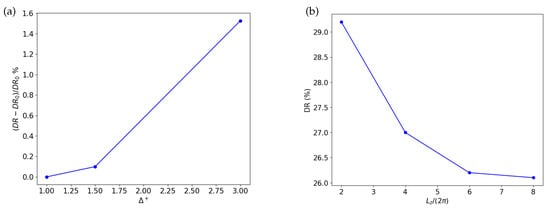
Figure 1.
Panel (a): Drag reduction error as a function of the grid spacing. Panel (b): Drag reduction as a function of the domain length.
A visual example of the flow configuration is provided by Figure 2, which shows the instantaneous contour of the velocity magnitude and the instantaneous configuration of the polymer position and shape (black lines; for the sake of visibility, only polymers in half geometry are represented).
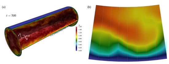
Figure 2.
Panel (a): Instantaneous snapshot of the velocity magnitude (contour plot) and the polymer conformation (black lines). Panel (b): Detail of the grid close to the wall. For the sake of visibility, the azimuthal grid points are represented with a skip equal to 7.
3. Results and Discussion
The addition of the polymers to the Newtonian solvent resulted in an increase in the flow rate. Figure 3a shows the mean axial velocity profile (angular parentheses denote the ensemble average) as a function of the wall distance . The inset shows the same data in wall units in a semi-log plot. The mean velocity profile is modified in the buffer layer and maintains a higher slope with respect to the unladen case, also in the logarithmic layer. The Von Karman constant is modified from to the value of in the polymer case. Overall, the polymers produced an increase in the mean axial velocity, resulting in a flow rate increase of the order of . The drag reduction can be estimated by defining the DR parameter in terms of the friction coefficient of the unladen and laden cases,
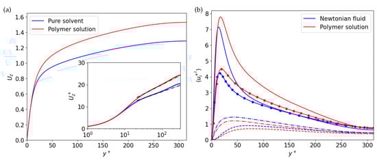
Figure 3.
Comparison between Newtonian flow and a polymer solution. (a) Mean velocity profiles, (b) Root mean square velocity statistics. : Solid line. : Dashed line. : Dot-dashed line. Turbulence intensity : Solid line with filled circles.
According to the definition, the drag reduction is of the order of . A comparison with the result reported in [13] ( at ) denotes that the amount of drag reduction is almost unaffected by the increase in the Reynolds number.
Figure 3b shows that the addition of the polymers produced a depletion of the spanwise and wall-normal velocity fluctuations and an increase in the axial velocity fluctuations . Overall, the effect on the turbulence intensity, the sum of the three terms, increased along the pipe radius. Besides the changes in the magnitude, the peaks of all the quantities reported in Figure 3b moved towards the pipe centre, which is in accordance with the increase in the buffer layer size captured by the experiments in [5] and the numerical simulations of viscoelastic flows in [7,11].
By integrating the mean axial momentum equation into the volume of the pipe, the classical stress balance can be recast as follows:
The viscous stress , the Reynolds stress , and the polymer extra stress are reported in Figure 4 together with their sum and the sum of the polymer and Reynolds stresses. The Reynolds stress of the Newtonian unladen case is also reported for reference purposes (black dashed line). In the laden case, the polymers produced a decrease in the Reynolds stress and an additional contribution representing the polymer back reaction on the fluid. Despite this additional stress, the sum is lower than the unladen Reynolds stress in both the buffer layer and the log layer, while it peaks further from the wall with respect to the Newtonian case. The modification of the stresses, i.e., of the streamwise momentum flux towards the wall, gives reason for the alteration of the mean velocity profile, which ultimately leads to drag reduction. We observed that, in contrast to the theory proposed by Virk, the presence of the polymers was felt all across the pipe section. Indeed, the mean velocity profile also had a different slope in the logarithmic layer, see Figure 3b.
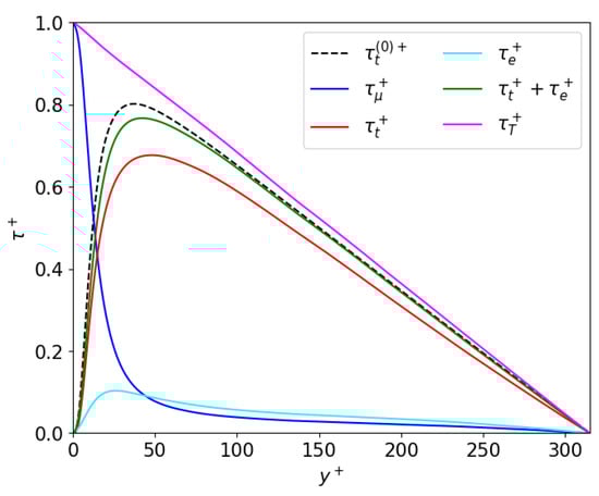
Figure 4.
Radial profile of stresses. The Newtonian unladen Reynolds stress (black dashed line) is reported for reference purposes.
The effects on the fluid described above are due to the polymer feedback on the carrier phase. Since the feedback force is strongly dependent on the polymer extension, it is useful to analyse the statistical properties of the polymer conformation by means of the probability density functions (pdf) of the end-to-end vector, see Figure 5. Panels (a)–(d), which correspond to different components of the end-to-end vector, show that the pdfs peak at the maximum length, independently of the distance from the wall, testifying that a large fraction of the polymer population (≈) is stretched to the limit. This effect is shown to be crucial for drag reduction at large Weissenberg numbers [13]. These numerical simulations also show that only the fully extended polymers contribute to the feedback reaction. The probability distributions of the three components of the end-to-end vector also highlight the preferential orientation of the polymer forcing. Note that only the right side of the pdf is displayed because of symmetry.
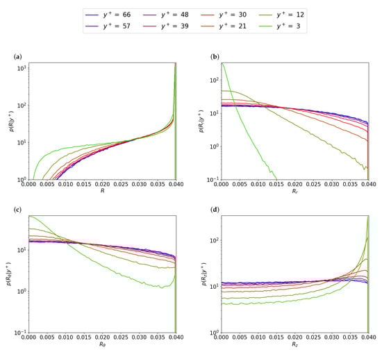
Figure 5.
Probability density functions of the polymer end-to-end vector conditioned to different distances from the wall. Panel (a): End-to-end length. Panel (b): Radial component. Panel (c): Tangential component. Panel (d): Axial component.
In the viscous and buffer layers, the most probable configuration consists of fully extended polymers aligned with the direction of the mean flow, whilst the polymer conformation, and thus the polymer back reaction, becomes more isotropic while approaching the pipe centre.
4. Conclusions
The direct numerical simulation of a polymer-laden turbulent pipe flow at high Weissenberg and Reynolds numbers was used to investigate the drag reduction phenomenon. An Eulerian–Lagrangian approach was employed by tracking every single polymer as a massless dumbbell and then considering their back reaction on the carrier fluid. The approach was able to overcome the limitations of the constitutive Eulerian–Eulerian-based models such as the FENE-P and allowed for the simulation of realistic polymer macromolecules at concentrations comparable to actual experiments.
The polymers contributed to the increase in flow rate at a fixed pressure drop corresponding to . The drag reduction was of the order of , which is similar to the one obtained at , showing a weak dependence on the Reynolds number.
Concerning the turbulent fluctuations, the turbulent kinetic energy increased, which was accompanied by an increase in the anisotropy of the flow. Indeed, the polymers increased the axial velocity component and decreased the others. The origin of the drag reduction had to be searched in the modification of the stress balance. The Reynolds stress was depleted by the polymer phase, and despite the appearance of an additional contribution, the sum of the Reynolds and the polymer stresses did not overcome the Newtonian Reynolds stress. The overall momentum flux towards the wall decreased with respect to the pure solvent, which led to the modification of the mean axial velocity profile and the increase in flow rate.
Finally, the analysis of the polymer conformation showed that the majority of the polymers were fully stretched and mainly aligned along the mean flow direction in the buffer and viscous layers, whilst in the log and outer layers, the chain conformation was almost isotropic.
Author Contributions
Conceptualization, F.B. and P.G.; software, F.S. and F.B.; data curation, F.S.; writing—original draft, F.S. and F.B.; Visualization, F.S.; writing—review and editing, P.G. and C.M.C.; supervision, P.G. and C.M.C.; funding acquisition, P.G. and C.M.C. All authors have read and agreed to the published version of the manuscript.
Funding
This work was partially supported by the Sapienza 2021 Funding Scheme, Project #RG12117A66DC803E.
Data Availability Statement
Not applicable.
Acknowledgments
We acknowledge the CINECA award under the ISCRA initiative, Iscra B number HP10B0F5V3, for the availability of high-performance computing resources.
Conflicts of Interest
The authors declare no conflict of interest. The funders had no role in the design of the study; in the collection, analyses, or interpretation of data; in the writing of the manuscript, or in the decision to publish the results.
References
- Toms, B. Proceedings of the 1st International Congress on Rheology; North Holland: Amsterdam, The Netherlands, 1949; Volume II, p. 135. [Google Scholar]
- Toms, B. On the early experiments on drag reduction by polymers. Phys. Fluids 1977, 20, S3–S5. [Google Scholar] [CrossRef]
- Marchioli, C.; Campolo, M. Drag reduction in turbulent flows by polymer and fiber additives. KONA Powder Part J 2021, 38, 64–81. [Google Scholar] [CrossRef]
- McComb, W.; Rabie, L. Local drag reduction due to injection of polymer solutions into turbulent flow in a pipe. Part I: Dependence on local polymer concentration. AIChE J. 1982, 28, 547–557. [Google Scholar] [CrossRef]
- Virk, P.S. Drag reduction fundamentals. AIChE J. 1975, 21, 625–656. [Google Scholar] [CrossRef]
- Berman, N.S. Flow time scales and drag reduction. Phys. Fluids 1977, 20, S168–S174. [Google Scholar] [CrossRef]
- Sureshkumar, R.; Beris, A.N.; Handler, R.A. Direct numerical simulation of the turbulent channel flow of a polymer solution. Phys. Fluids 1997, 9, 743–755. [Google Scholar] [CrossRef]
- Bird, R.B.; Curtiss, C.F.; Armstrong, R.C.; Hassager, O. Dynamics of Polymeric Liquids, Volume 2: Kinetic Theory; Wiley: New York, NY, USA, 1987. [Google Scholar]
- Dubief, Y.; Terrapon, V.E.; Hof, B. Elasto-Inertial Turbulence. Annu. Rev. Fluid Mech. 2022, 55, 2023. [Google Scholar] [CrossRef]
- Dimitropoulos, C.D.; Sureshkumar, R.; Beris, A.N. Direct numerical simulation of viscoelastic turbulent channel flow exhibiting drag reduction: Effect of the variation of rheological parameters. J. Non-Newton. Fluid Mech. 1998, 79, 433–468. [Google Scholar] [CrossRef]
- De Angelis, E.; Casciola, C.; Piva, R. DNS of wall turbulence: Dilute polymers and self-sustaining mechanisms. Comput. Fluids 2002, 31, 495–507. [Google Scholar] [CrossRef]
- Zhou, Q.; Akhavan, R. A comparison of FENE and FENE-P dumbbell and chain models in turbulent flow. J. Non-Newton. Fluid Mech. 2003, 109, 115–155. [Google Scholar] [CrossRef]
- Serafini, F.; Battista, F.; Gualtieri, P.; Casciola, C. Drag Reduction in Turbulent Wall-Bounded Flows of Realistic Polymer Solutions. Phys. Rev. Lett. 2022, 129, 104502. [Google Scholar] [CrossRef] [PubMed]
- Gatignol, R. The Faxén formulae for a rigid particle in an unsteady non-uniform Stokes flow. J. Mec. Theor. Appl. 1983, 2, 143–160. [Google Scholar]
- Maxey, M.R.; Riley, J.J. Equation of motion for a small rigid sphere in a nonuniform flow. Phys. Fluids 1983, 26, 883–889. [Google Scholar] [CrossRef]
- Picardo, J.R.; Singh, R.; Ray, S.S.; Vincenzi, D. Dynamics of a long chain in turbulent flows: Impact of vortices. Philos. Trans. R. Soc. A 2020, 378, 20190405. [Google Scholar] [CrossRef] [PubMed]
- Choi, H.; Lim, S.; Lai, P.Y.; Chan, C. Turbulent drag reduction and degradation of DNA. Phys. Rev. Lett. 2002, 89, 088302. [Google Scholar] [CrossRef] [PubMed]
- Gualtieri, P.; Picano, F.; Sardina, G.; Casciola, C.M. Exact regularized point particle method for multiphase flows in the two-way coupling regime. J. Fluid Mech. 2015, 773, 520–561. [Google Scholar] [CrossRef]
- Battista, F.; Mollicone, J.P.; Gualtieri, P.; Messina, R.; Casciola, C.M. Exact regularised point particle (ERPP) method for particle-laden wall-bounded flows in the two-way coupling regime. J. Fluid Mech. 2019, 878, 420–444. [Google Scholar] [CrossRef] [PubMed]
- Li, N.; Laizet, S. 2decomp & fft-a highly scalable 2d decomposition library and fft interface. In Proceedings of the Cray User Group 2010 Conference, Edinburgh, UK, 24–27 May 2010; pp. 1–13. [Google Scholar]


Publisher’s Note: MDPI stays neutral with regard to jurisdictional claims in published maps and institutional affiliations. |
© 2022 by the authors. Licensee MDPI, Basel, Switzerland. This article is an open access article distributed under the terms and conditions of the Creative Commons Attribution (CC BY) license (https://creativecommons.org/licenses/by/4.0/).