Abstract
In this paper, we numerically investigate the turbulence modulation produced by long flexible fibres in channel flow. The simulations are based on an Euler–Lagrangian approach, where fibres are modelled as chains of constrained, sub-Kolmogorov rods. A novel algorithm is deployed to make the resolution of dispersed systems of constraint equations, which represent the fibres, compatible with a state-of-the-art, Graphics Processing Units-accelerated flow-solver for direct numerical simulations in the two-way coupling regime on High Performance Computing architectures. Two-way coupling is accounted for using the Exact Regularized Point Particle method, which allows to calculate the disturbance generated by the fibers on the flow considering progressively refined grids, down to a quasi-viscous length-scale. The bending stiffness of the fibers is also modelled, while collisions are neglected. Results of fluid velocity statistics for friction Reynolds number of the flow and fibers with Stokes number = 0.01 (nearly tracers) and 10 (inertial) are presented, with special regard to turbulence modulation and its dependence on fiber inertia and volume fraction (equal to · and ·). The non-Newtonian stresses determined by the carried phase are also displayed, determined by long and slender fibers with fixed aspect ratio , which extend up to the inertial range of the turbulent flow.
1. Introduction
The transport of fibers by a turbulent flow is the subject of ongoing research because of its relevance in many industrial applications, such as pulp and paper production [1], pharmaceutical processing [2], post-combustion filtering [3] and drag reduction in oil pipelines [4]. In addition, fiber transport by turbulence is common to a number of environmental and natural processes, such as the dynamics of plankton in the oceans, the formation of icy particles in clouds and the dispersion of pollen in the atmosphere [5]. In all of these systems, fibers are rotating and their interaction with the flow strongly depends on the fiber orientation relative to the flow at a microscopic level [6,7,8,9]. This gives rise to a physics-rich phenomenology at the macroscopic level, which culminates in the modification of the overall drag associated to the turbulent flow. When this modification is favorable, a beneficial effect is obtained (drag reduction) since the flow rate can be increased while keeping the same driving pressure gradient. The first study of drag reduction dates back to the pioneering work of Forrest and Grierson on wood pulp fiber suspensions [10], and was later reported to the international community by Toms, after his experiments with dispersed polymers in pipes [11]. Polymers are macromolecules that can coil and have sizes smaller than the Kolmogorov length scale, which is the smallest scale in a turbulent flow. In this study, however, we are interested in the drag-reducing capabilities of fibers with size larger than, or at least equal to, the Kolmogorov length scale. The main advantage of using fibers as drag-reducing agents is that fibers exhibit chemical and mechanical stability over a wider range of temperatures compared to polymers; the disadvantages are a lower effectiveness in reducing drag and the risk of plugging the pipelines where they are dispersed [12].
Motivated by possible applications in oil pipelines and deep-operating flooded motors, many experimental studies followed the two above-mentioned seminal works and produced a large qualitative characterization of drag reduction both by polymers [13,14] and by fibers, especially in the limit of very high aspect ratio i.e., the ratio between the fiber length and the fiber diameter [15]. In these early works, the explanation for drag reduction was associated with the occurrence of extra stresses of non-Newtonian nature within the flow (due to the presence of the drag-reducing agent) even at low concentrations of few hundreds of PPM in weight. Moreover, polymers appeared to reduce the coupling between the axial and the wall-normal components of the turbulent flow field by being continuously stretched from their coiled state: this effect was observed to be particularly strong near the walls, where the polymers are found to interfere with the turbulent bursts directed towards the bulk of the flow [16]. On the other hand, fibers appeared to have a broader range of influence since their resistance to extensional deformations allows to produce a favorable effect even in the core of the flow [17,18,19]. However, subsequent experiments with asbestos rigid rods with estimated aspect ratio of 40,000 showed higher drag-reduction efficiencies when injecting the drag-reducing agent near the wall rather than in the bulk of the flow [20]. Interestingly, polymers and fibers were also found to be more effective when acting in combination rather than in isolation, also in the dilute regime [21].
While early experiments could produce a qualitative description of the phenomenology of drag reduction, the first numerical studies could be performed only much later due to the computational costs of simulating a polymer-/fiber-laden turbulent flow. The simulation task is made particularly difficult not only by the anisotropies associated with both the (wall-bounded) flow and the (non-spherical) polymers/fibers, but also by the need to account for the polymer/fiber disturbance on the flow, which ultimately determines drag modulation and requires proper modelling of the two-way coupling between the phases. Two-way coupled direct numerical simulations with rod-like fibers as drag-reducing agents, were performed by Paschkewitz et al. [22] and by Gillissen et al. [23], who reported an increase of axial turbulent intensities and a decrease of the wall-normal ones, resulting in a modified momentum balance where a new term, the axial-wall normal fiber stress, appears to take over the role that Reynolds stresses (weaker in two-phase turbulence) have in single-phase turbulence. The modelling approach adopted in these two studies is quite similar, since neither of the two did actually resolve the motion of the fibers in a Lagrangian fashion, but rather relied on the knowledge of the orientation probability to obtain a local expression for the fiber-induced stresses feed-backing on the flow. The clear advantage of this approach is provided by the reduced computational effort, albeit at the cost of being applicable only to sub-Kolmogorov, inertia-less polymers that are stretched and do not coil, or very short fibers. Following these purely Eulerian investigations, direct numerical simulations based on the Eulerian–Lagrangian approach started to appear in the literature. In these simulations, dense suspensions were considered and the dynamics of the dispersed phase was directly resolved to calculate the non-Newtonian stresses exerted on the flow, either based on a Monte Carlo approach [24] or derived as a sum of stresslets [25]. These simulations granted higher accuracy in determining the axial-wall normal particles stress on the flow and, in turn, the actual drag reduction (which could be easily miscalculated using Eulerian closure methods). However, the two-way coupling method employed in these works (which requires a normalization over local flow volumes to compute the disperse phase feedback force on the turbulence to be performed) suffers from several drawbacks. Firstly, the back-reaction field, that can be constructed given the configuration of the suspension, is grid dependent and the solution depends on how many particles per computational cell are available. The constraint on the number of particles per cell was found to limit the range of the dimensionless parameters (Stokes number, mass loading, particle-to-fluid density ratio and Reynolds number) that can be explored in the simulations [26]. In particular, the method is not accurate in the case of dilute suspensions, when fiber-induced drag reduction was observed to occur even at low volume fractions [15,21]. A further issue concerns the model used to compute the hydrodynamic forces acting on each particle. In the simplest Stokes drag model, the fluid velocity at the particle position must be the fluid velocity in absence of the disturbance flow produced by the dispersed phase. Unfortunately, such a velocity is unavailable in two-way coupled simulations, and specific techniques must be exploited to remove the particle self-disturbance [26].
Motivated by the interest to investigate numerically turbulent drag reduction in dilute fiber suspensions, and by the need to go beyond classic two-way coupling methods, in this manuscript we present a series of momentum-coupled, Euler–Lagrangian direct numerical simulations of fiber-laden turbulent channel flow. The two-way coupling linear momentum is calculated according to the Exact Regularized Point Particle method [26], a rigorous method proposed recently to circumvent the necessity of considering a large number of fibers at the price of highly resolved calculations. Then, we extend the work of Dotto et al. [27], in which flexible fibers were considered, modelled according to the rod-chain model [28,29,30]. In this work, fibers are composed of a series of point-wise, sub-Kolmogorov rods constrained together to achieve an overall fiber length that extends in the inertial range of turbulent scales [31] and to allow deformation through relative rotation of neighboring rods. An instantaneous visualization of the resulting flow is shown in Figure 1, where fibers are shown together with the flow structures with which they interact (rendered using iso-surfaces of the second invariant Q of the velocity gradient tensor).
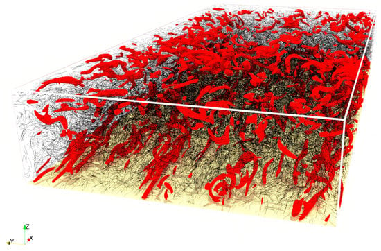
Figure 1.
Instantaneous visualization of the fiber-laden turbulent channel flow considered in this study. Flow structures are rendered as iso-surfaces of the second invariant Q of the fluid velocity gradient tensor (the selected value is , corresponding to one tenth of the maximum value of Q obtained in the simulations); the diameter of the fibers is enhanced by a factor of three for visualization purposes. The upper wall of the channel is transparent for visualization purposes.
The length of the fiber is a crucial parameter of the simulations, as it is known that long fibers feel less the contribution of the smallest turbulent structures due to local averaging along their shape [32]. Therefore, a strong impact on the non-Newtonian stresses so generated should be expected. We considered a fixed value of the fiber aspect ratio, namely : This value is enough to generate fibers with length comparable to the scales of turbulence in the inertial range for the specific shear Reynolds number we simulated () and yet is two orders of magnitude lower than that considered in previous experiments [15,20]. In addition, the fiber length considered in our study is equal to 0.6 times the wall-to-wall distance of the computational domain (assuming that the fiber is fully stretched): this value is significantly higher than that typically investigated in experiments, e.g., ∼0.07 in the pipe flow experiment of Sharma [20]. Clearly, computational costs limit our exploitable parametric space. Nevertheless, as we will show, it is in an appreciable drag reducing dispersion of fibers.
The manuscript is organized as follows. First, we give an overview of the physical problem, its governing equations and the numerical method used to solve them (Section 2), focusing on the importance of including two-way coupling to retrieve experimentally-validated results. Then we move on to the discussion of flow visualizations and statistical observables that allow a characterization of the flow modulation (Section 3). Finally, the main conclusions and future developments are provided in Section 4.
2. Materials and Methods
2.1. Flow
The carrier phase is an incompressible Newtonian fluid, flowing between two smooth, parallel walls in a plane channel. The flow is driven by an imposed pressure gradient and can be described by the coupled system of Continuity and Navier–Stokes equations, which in dimensionless vector form read as:
where is the velocity vector at the position , is the equivalent pressure gradient that drives the flow, is the shear Reynolds number, whereas the term represents two-way coupling momentum term that the dispersed phase exerts on the flow. This term is calculated according to the ERPP method [26], and will be presented in detail in Section 2.3 of this manuscript.
The shear Reynolds number of the flow is defined as , with the fluid density, the fluid dynamic viscosity, the shear velocity (computed based on the mean wall shear stress, ) and h the half-height of the channel. The flow is resolved down to the smallest scales performing a direct numerical simulation on an Eulerian grid that discretizes a rectangular box of size in the streamwise direction x, in the spanwise direction y and in the wall-normal direction z. The numerical method used by the flow solver is based on a classical pseudo-spectral algorithm, where all the calculations are performed in the Fourier–Chebyshev modal space, except for the convective terms , which are resolved in physical space and then back transformed in modal space [33]. The governing equations (conservation of mass and momentum) are solved in their velocity-vorticity formulation by projecting along the wall-normal coordinate and calculating the respective vorticity and velocity w components. From these, the remaining velocity components u and v are then obtained. Time integration is performed using a mixed implicit-explicit scheme: the linear and non-linear terms of the Navier–Stokes equations are split, so that a Crank–Nicolson implicit scheme is employed to calculate the former, whilst an Adams–Bashforth explicit scheme is employed to calculate the latter. Note that the two-way coupling force is added to the non-linear terms before integration. The solution is advanced in time on an Eulerian grid, partially displayed in Figure 2: The grid spacing is uniform along the homogeneous directions (represented by the x and y coordinates), while Chebyshev polynomials are employed along the wall-normal direction to obtain a suitably-fine grid discretization near the walls. Finally, periodic boundary conditions are imposed in x and y, while a no-slip boundary condition is enforced at the two walls.
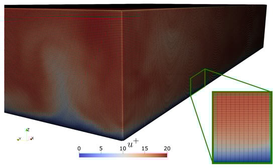
Figure 2.
Visualization of the Eulerian grid adopted in our simulations over half of the channel height. Grid points are located at the intersection between black lines. The grid spacing in the streamwise x and spanwise y coordinates is uniform, and is simply determined by the chosen number of points (). Chebyshev polynomials, given by the following expression, , with allow to obtain a much finer grid discretization close to the wall, as we can appreciate from the small insert. In the simulations presented in this manuscript the minimum spacing is at the wall, while the maximum value is at the center of the channel.
2.2. Fibers
Fibers are modelled using the rod-chain model [27,28,29,30]. According to this model, multiple sub-Kolmogorov rod-like elements are constrained together to form long, flexible fibers. The main advantage of this model is that, as each rod element is shorter than the smallest (Kolmogorov) flow scale, the surrounding flow can be linearized. By doing so, the torques acting on each rod can be directly calculated using the viscous theory derived by Jeffery [34] for ellipsoidal particles, and later extended to fibers by the semi-empirical correlation of Cox [35] in its generalization to three-dimensional flows [36].
As shown in Figure 3, the nth rod element of each fiber is treated as a point-wise object to calculate its translation and rotational dynamics: its position will be provided by the unit norm vector , its orientation will be given by a unity norm vector and its linear and angular velocities will be reported as and . The mass of the rod is , where is its density, a its radius and its aspect ratio, defined as the ratio between the rod half length ℓ and cross-sectional radius a. The governing dynamic and kinematic equations for the linear and angular motions of the rod read as follows:
where is the hydrodynamic drag force exerted by the fluid on the element, is the inertia tensor of the element in the absolute frame of reference, with the identity matrix. The term is the hydrodynamic torque due to the relative spin between fluid and rod element and the term is the hydrodynamic torque due to the fluid velocity gradients’ action of the rod. Finally, the extra terms and represent the constraint forces and moments that consecutive rods belonging to the same chain exert on each other, as shown in Figure 4. These terms arise from the enforcement of a no-slip constraint between the rod pair, given by the following condition:
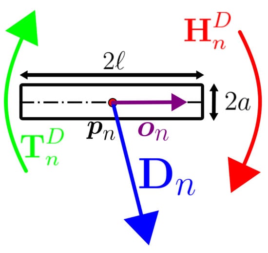
Figure 3.
Representation of a pointwise rod element of length and cross-sectional diameter . The force and the torques and exerted by the surrounding flow on the element are also shown, together with the position unit vector and the orientation unit vector .
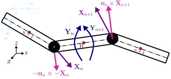
Figure 4.
Schematic representation of three constrained, pointwise rod elements with the constraint forces and torques.
Note that the constraint forces alone would be sufficient to keep the chains of rods together. Therefore, the role of the moments is simply to keep the rod elements aligned, and the generic torque determined by the relative orientation between the th and the nth rod element is given by the following expression:
where the Young modulus of the material appears, as well as the solid angle between two consecutive elements, , and their relative curvature, .
Therefore, Equations (2a–d) and (3) combined together determine a tridiagonal block-matrix system. Its resolution requires the following steps to be taken:
- an interpolation of the flow velocity components and velocity gradients at the center of gravity of each rod-like element of the fiber to determine the force and the torques exerted by the surrounding fluid on the element, which we calculated using fourth order polynomials;
- the resolution of a tridiagonal block-matrix system to determine the constraint forces on each element over all the tracked fibers (chains);
- time integration of the kinematic equations of each element of each fiber, which perform using a second order Adams–Bashforth scheme to determine the position and the orientation of the element itself;
- detection of collisions between a given element of the fiber and the walls, modelled as an elastic impact with unitary restitution coefficient, in which the sign of the wall-normal velocity of the element is changed;
- verification of the accuracy of the time integration with special regards towards the accumulation of numerical error between constrained elements and correction.
This last step is of particular importance [29,37], and was performed by fixing the position of the middle element of the chain and translating the other rods around it, in order to reproduce the exact fiber length and avoid accumulation of numerical errors. Each chain of rods must then meet a maximum constraint error, which distinguishes between valid and invalid solutions. To accomplish this verification, a sub-stepping procedure is introduced, in order to improve the stability of the model, particularly critical when simulating large values of the Young modulus and/or short rod-like elements.
Besides stability issues, the time integration of fiber motion is dominated by the fiber shape and density ratio with respect to the fluid. These two parameters are combined to determine the response time of the generic element of the chain [27]:
Fibers characterized by a negligible response time behave as tracers in the flow, whereas fibers characterized by with high values of the response time exhibit a more ballistic behavior. Finally, gravity is not taken into account in the present simulations, so that the inertial behavior of the fibers is purely hydrodynamic.
2.3. Two-Way Coupling
The pointwise modelling adopted for tracking the fibers neglects the boundary condition that finite-size fibers would impose on the flow. This modelling assumption is clearly necessary given the need to simulate a large number of fibers and hence elements (up to two million). Even within this limit, however, it is possible to recover the fiber back-reaction to the fluid as the Newtonian reaction to the drag force . Intuitively, each fiber contributes to the back-reaction within a finite volume of the flow, so that the sum of all reaction forces determines the normalized force that appears in the Navier–Stokes Equation (1b). The method just described is known as the Particle In Cell method, originally proposed by Squires et al. [38] and largely employed since, due to its simplicity. However, the method requires the presence of a very large number of particles within the control flow volume over which the two-way coupling force is normalized in order not to diverge. Because of this requirement, accurate calculation of the particle stresses on the turbulent flow requires extremely high (sometimes unfeasible) computational resources [39]. Therefore, in this work (in which particle concentrations are not particularly large) another method of more recent derivation is employed, namely the Exact Regularized Point Particle method [26] in its generalization to wall-bounded turbulent flows [40]. The details of this method are briefly described in the following.
The ERPP method provides a rigorous derivation based on the unsteady Stokes flow around a small, spherical, rigid particle, whose interaction with the flow is physically regularized by viscous diffusion, that slowly propagates the generated vorticity field from the particles boundary to the computational grid, as shown in Figure 5. To account for this, the method introduces a delayed time-scale, , below which the particle’s disturbance has yet to interact with the flow and can be neglected without incurring a large error. The resolution of such time-scale imposes a length-scale that the computational grid needs to discretize:
where indicates the fluid kinematic viscosity. In the end, each particle-delayed hydrodynamic force will be the one calculated at a slightly previous time-step , when the particle was at the position , regularized by means of a Gaussian whose variance is indeed . The summation of the contribution of all particles gives:
where is the total number of simulated rods and the Gaussian corresponds to the following expression:
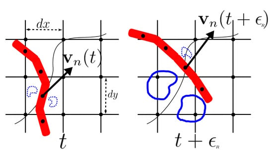
Figure 5.
Schematic representation (freely inspired by [26]) of the two-way coupling according to the ERPP method. Left panel: the disturbance generated by the element moving with velocity at the time-step t has yet to diffuse to the computational grid, whose spacing is indicated by and . Right panel: At time , the element has moved along its trajectory while the previously generated disturbance has diffused enough to reach the computational grid with delay .
In summary, the ERPP method consists of an extra step that can be easily added to any flow solver for multiphase numerical simulations. As displayed in Figure 6, the method only requires to store, since the start of the simulation and over a suitably-long time window, the position of each element composing the fiber and the drag force experienced by the element. Then, once the delayed time scale has expired, the two-way coupling term can be calculated and added as a source term in the governing equations for the fluid, Equation (2a,b). The array in which and are stored is finally updated, removing the oldest data in the chronology and replacing it with the data at the current time step, thus allowing for advancement of the equations to the next time step.
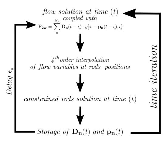
Figure 6.
Schematic representation of the method of study: all the simulations performed in this study start from a random dispersion of mean-flow-aligned fibers at a given volume fraction in fully-developed turbulent channel flow. Then, the calculations are advanced in time, storing the instantaneous position of each fiber element, , and the drag force experienced by the element, over a time window whose length is given by the ratio between the delayed time scale and the value for the time step, . Once one full delayed time scale has expired, the two-way coupling term can be calculated and added as a source term in the governing equations for the fluid, . The loop is then repeated until the end of the simulation.
2.4. Implementation
The governing equations for the two phases are implemented in a proprietary flow and particle solver that is written in CUDA C for accelerated computing on Graphics Processing Units. The Eulerian flow solver can handle Fourier–Chebyshev transforms between physical and modal spaces by relying on the CUFFT library, whereas all other solver subroutines have been developed in-house.
Single-GPU optimization is obtained by accessing the data in slabs, to minimize the impact of complex operations along the non-homogeneous coordinate z, such as derivatives and solution of systems of equations, which carry embedded data dependencies and would be extremely cumbersome in terms of coalescent memory access [41]. Then, multi-GPU execution is coordinated by standard Message Passing Interface (MPI), according to a classical mono-dimensional domain decomposition, where the data synchronization is managed through collective asynchronous calls to maximize overlap between calculations and communications. The Lagrangian fiber tracking solver, instead, is written in Fortran 90 and parallelized by OpenMP for multi-core execution. The entire chains of rods are resolved locally and the compatibility with the flow-solver is ensured by an asynchronous algorithm, in order to correctly sample the Eulerian grid when performing (a) the fourth-order interpolation of the flow variables at the position of the center of mass of each rod, and (b) the diffusion of the fibers disturbance. This is done by a second copy of the rod elements that is travelling within the distributed memory units among which the Eulerian grid is parallelized: synchronization between the two copies of each element is then ensured by two collective communication moments, in correspondence with operations (a) and (b), where data is shared on demand according to the highly unpredictable conformation of each fiber. All these features are combined to give a scalable application, suitable for execution on large, distributed computational architectures: to the best of our knowledge, this is the first time that a similar algorithm is employed for fiber-laden turbulent flows.
2.5. Validation
A classic test-case for the validation of a fiber-laden flow solver in the two-way coupling regime consists of replicating the rotation of one fiber in a simple viscous shear flow. If in an iso-density condition, the fiber will undergo periodic rotations, while each of its ends describes a closed orbit, known as Jeffery orbit (it was G. B. Jeffery who was the first to provide an analytical description of the phenomenon for ellipsoidal particles [34]). The period of rotation for the fiber is given by the following expression:
where is the shear rate of the viscous shear flow.
Great care must be taken to simulate rod-like fibers as these are characterized by an equivalence of shape with respect to ellipsoidal fibers. This equivalence is such that the rod-like fibers exhibit a shorter period of rotation compared to ellipsoidal fibers, as observed experimentally and rationalized by the semi-empirical correlation of R. G. Cox [35]:
where the equivalent aspect ratio that will give the correct period of rotation of a rod-like fiber, , through Equation (9) is related to the aspect ratio of the ellipsoidal fiber, , for which the theoretical calculation of the rate of strain and rate of rotation torques is given.
We validate our implementation of the ERPP method against the period of rotation of fibers in viscous shear flow, using the length-scale given by Equation (6) and considering progressive refinements of the computational grid. Such a validation is performed at friction Reynolds number by imposing a zero pressure gradient in the Navier–Stokes solver as well as no-slip boundary conditions at the two walls, which are now moving with imposed constant velocity in opposite directions. The equations that describe the flow and the fibers can be normalized in terms of the relevant scales at the wall so that dimensionless quantities in these equations are indicated by the superscript +. By doing so, a dimensionless quantity that appears in the fiber equation of motion is the Stokes number, defined here as the ratio between the characteristic time scale of the generic element of the fiber and the characteristic time scale of the flow, :
This parameter can be compared to time-scale , introduced by the ERPP method, and directly determined by the resolution of the computational grid. By doing so, we can estimate the optimal resolution, fine enough to produce an experimentally validated solution for the Jeffery orbits of the fiber, but also not so computationally expensive to result in unfeasible simulations when these are applied to turbulent flows.
The coarser Eulerian grid adopted for the one-way coupling is perfectly affordable from a computational cost perspective, being made of points. However, despite having imposed the Cox equivalence for each rod-like element, the recovered solution for the whole fiber clearly overestimates the period of rotation, displayed as empty blue squares in Figure 7. A first refinement, obtained by increasing the the number of grid points in each direction by a factor of 2 and by activating the two-way coupling, results in a ratio of 90 between the ERPP time-scale and the element Stokes number, shown as green empty diamonds in Figure 7. We can appreciate a first impact of the two-way coupling, which slightly reduces the period of rotation. Finally, refining once more the number of grid points by a factor of 2 in each direction, the ratio becomes equal to 5, and the solution, displayed as orange empty diamonds in Figure 7, perfectly recovers the semi-empirical correlation of Cox [35]. In conclusion, the two-way coupling is crucial to obtain a correct solution, in agreement with what reported by Lindstrom et al. [29]. This is especially true when the ratio between the particle characteristic time-scale and the grid-resolved time-scale is small. The criterion just discussed has been used to estimate the scale up of our calculations and the Eulerian grid needed to properly simulate the targeted fiber-laden turbulent channel flow in the two-way coupling regime.
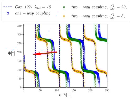
Figure 7.
Time evolution of the angle , defined as the angle between the gradient direction of a viscous shear flow and the particle orientation vector. Here, the fiber is assembled as a chain of five rods of aspect ratio so that the total aspect ratio is ; bending is avoided by imposing a large-enough value of the Young modulus. The dotted curves represent the Jeffery orbits, obtained from calculations over progressively refined grids, while the dashed line is the analytical solution, obtained from Jeffery theory [34] through the equivalence of shape of Cox [35]. The red arrow indicates the progressive refinements of the Eulerian grid: A grid refinement of on the number of grid points is introduced between each solution.
3. Results
3.1. Summary of the Simulations
In this work, we present the results of four different simulations. Each fiber is made of 40 rod-like elements of aspect ratio . The length of the fibers is thus fixed to in wall units and their aspect ratio to , while their inertia and average volume fraction are varied according to Equation (11). In particular, we consider a low-inertia case, in which each element has and , and a high-inertia case, in which each element has and . We note here that the Stokes number of each rod-like element can be intuitively associated to the Stokes number of the entire fiber (namely the entire chain of rods) when the fiber is in its fully stretched equilibrium configuration and assuming that all elements have the same density. In this specific instance, the total Stokes number becomes ∼0.05 for the low-inertia case and ∼50 for the high-inertia case. These two cases correspond to an average volume fraction of and , respectively. In turn, these volume fractions correspond to a dispersion of = 200,000 and = 2,000,000 elements having each a dimensionless volume . The corresponding by weight can be calculated as:
resulting in 27.5 and 275 for the low-inertia case and in 21,605 and 216,055 for the high-inertia case. Elaborating on the considerations made previously about the discrepancy of fiber concentrations between experiments and numerical studies, we want to highlight here that the mass loadings for the low-inertia fibers are directly comparable with the experiments of Hoyt [15]. The considered values differ substantially from previous numerical studies, which refer to simulated mass loads at least one decade larger than what presented in the present study.
The Navier–Stokes and Continuity Equations (2a–d) are integrated on a computational grid made of points. This allows to set the dimensionless regularization length-scale required by the ERPP method to , which gives a ratio , where represents the grid spacing for the ith direction. Eventually, this produces a delayed time-scale wall time units. Therefore, the drag force acting on each fiber element and the position of the center of mass of each element are stored for 108 time-steps before the corresponding disturbance can be calculated. We can compare the dimensionless characteristic response time of the individual rod-like elements or that of the full chain, Equation (11), with this delayed time-scale, so that if the latter is smaller than the former, the accuracy of the validation in simple viscous shear flow is maintained when considering large-scale turbulent channel flow simulations. Clearly, this is the case for the inertial fibers, while a compromise between quality and computational cost had to be made for the tracer-like fibers. On a final note, we impose a constant value for the Young modulus: . This value enforces a minimal energy configuration for the fully-stretched chain and is sufficient to keep the individual elements of the chain aligned to each other in the shear flow validation tests. In the turbulent channel flow simulations, however, this value turns out to be not high enough to prevent fiber deformation and bending. Nevertheless, the influence of the Young modulus on the measured drag reduction will not be discussed in this manuscript, as it is a matter of ongoing investigation.
All the simulations start from a fully-developed turbulent flow condition. Fibers are injected into the flow as fully stretched and randomly dispersed, with initial orientation along the streamwise direction. After injection, fibers evolve in time under the action of the turbulent flow and eventually forget about the initial condition imposed on their conformation, position, orientation and velocity. The statistics discussed in the following were computed only after this independence was achieved. Calculations are performed on 64 Nvidia Tesla V100 cards of Marconi 100, hosted by CINECA (Italy). Thanks to the scalability properties of the computational solver, simulations at the lower volume fraction () require an elapsed time per time-step of approximately 400 milliseconds. The elapsed time per time-step doubles when the higher volume fraction () is simulated. The calculations are carried out until a linear profile of the total axial momentum balance is obtained [31], resulting in nearly 2000 (resp. 4000) GPU hours at the lower (resp. higher) volume fraction. Then, the flow field is sampled every 15 wall time units, gathering at least 100 fields to calculate the statistics discussed in the following. Great care was taken for the statistics referring to the inertial fibers, for which longer averaging windows are necessary to achieve convergence. Unless otherwise stated, all statistics are presented as functions of the wall-normal dimensionless coordinate . Averaging of the statistics is performed along the two homogeneous directions, applying the classical Reynolds decomposition of the velocity vector:
where the overbar indicates the mean component of the velocity vector, whereas the superscript indicates its fluctuating component.
3.2. Flow Visualization
A visual rendering of the modification of turbulence due to the presence of the fibers is provided in Figure 8, Figure 9, Figure 10 and Figure 11, each referring to a different simulation carried out in this study. For each figure, the Eulerian grid is horizontally cut at from the wall and the resulting slice is colored according to the local value of the streamwise fluid velocity. Fibers located within a distance of 20 wall units above the slice are also rendered. The actual fiber length is shown, whereas the fiber diameter is magnified by a factor of five for visualization purposes.
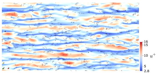
Figure 8.
Top view of the streamwise fluid velocity streaks in the near-wall region () and instantaneous fiber distribution. Reference simulation: .
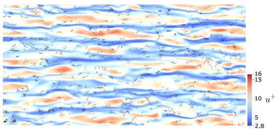
Figure 9.
Top view of the streamwise fluid velocity streaks in the near-wall region () and instantaneous fiber distribution. Reference simulation: .
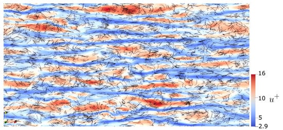
Figure 10.
Top view of the streamwise fluid velocity streaks in the near-wall region () and instantaneous fiber distribution. Reference simulation: .
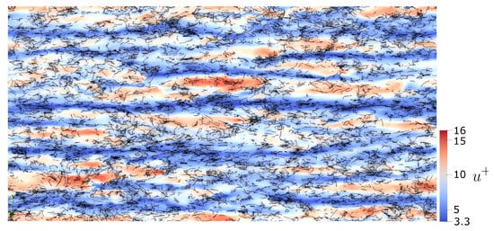
Figure 11.
Top view of the streamwise fluid velocity streaks in the near-wall region () and instantaneous fiber distribution. Reference simulation: .
The two cases at lower volume fraction, shown in Figure 8 for the fibers and in Figure 9 for the fibers respectively, already show some modification in the spatial distribution of the velocity streaks. These appear to be somehow weaker and characterized by a smoothing of the velocity field. Also, fibers seem to align along low speed streaks, in agreement with previous numerical studies [42], but in disagreement with the experiments of Shaik et al. [43].
As could be expected, the near-wall flow field modifications appear to be more evident at the higher volume fraction, as shown in Figure 10 for the fibers and in Figure 11 for the fibers respectively. The velocity streaks appear more regular and the spacing between them seems to increase, especially in the case of fibers with higher inertia, in accordance with numerical simulations of turbulence modulation by sub-Kolmogorov spheroids [25]. From a qualitative point of view, it can be observed again that fibers exhibit a preferential alignment in the low-speed streaks. This is especially visible in the case of inertial fibers, which are able to accumulate more efficiently than tracer-like fibers in the near-wall region by virtue of the turbophoretic mechanism that controls their wall-normal transport. In turn, this leads to an increase of the local (near-wall) volume and mass fractions, which generate a stronger feedback force from the fibers to the fluid.
A comment is in order about the conformation attained by the fibers as they are transported by the turbulent flow. Albeit characterized by a certain degree of bending stiffness, fibers are not able to maintain the initial conformation and cannot remain fully stretched. Rather, they undergo deformation and behave like flexible objects, as clearly displayed in Figure 12. In this figure, we isolate a relatively small volume of the flow domain to allow a real-scale rendering of the fibers, considering the simulation with inertial rods () at higher concentration () as reference. It is possible to appreciate a bundle of stretched fibers seemingly moving away from the wall, from left to right, probably due to a strong shearing event. Around them, instead, curved fibers can be observed, with the most likely conformation being that of a regularly bent object. Some extreme bending angles can be seen from time to time: An investigation of such extreme deformations, however, would require a discussion over the interplay between turbulence and fiber bending stiffness in the two-way coupling regime, which is beyond the purposes of the present work.
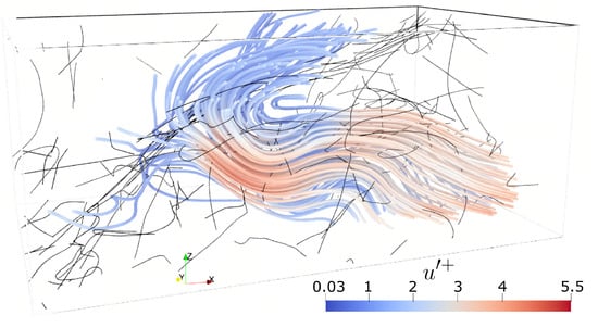
Figure 12.
Visualization of the flow streamlines within a volume of size in wall units, centered at a distance of 50 wall units from the wall (for the reference case of fibers and as volume fraction). The streamlines are colored according to the magnitude of the fluctuating fluid velocity. The fibers are also shown, rendered as thin black filaments.
3.3. Mean Velocity Profiles
The mean velocity profiles of the fiber-laden simulations are shown in Figure 13. To correctly compare these profiles with those of the unladen case, the velocity is normalized by the shear velocity obtained from the actual mean wall shear stress of the two-way coupled simulation. Only the streamwise velocity component u is plotted, as the other two components have zero mean. Our results indicates that there is a proportionality between the fiber volume fraction and the attained drag reduction, with a higher concentration of particles determining stronger reduction. This effect is more subtle for the inertial fibers. Apparently, an onset volume fraction is trespassed between the two simulations, which leads to a switch from drag increase in the low- case to drag reduction in the high- case. We can quantify these trends by defining the drag reduction percentage as done in [22]:
where the superscript L indicates the friction velocity obtained in the two-way coupled simulations while the superscript U indicates the same quantity for the unladen flow. As reported in Table 1, our results indicate a gentle drag reduction, except for one drag increase result. As a comparison, previous numerical investigations [22,23,24,25] reported a 10-times higher drag reduction percentage with a 10-times higher mass loading. The comparison with experiments is less satisfactory, as the measured drag reduction percentages reported in the literature are always larger than those reported in the table, even for the very low concentrations [15,21]. These discrepancies, however, can be ascribed to several aspects of the present simulations, among which two emerge. The first aspect is the flexibility of the simulated fibers, which are not perfectly rigid as those considered in the experiments. The second, and most relevant, aspect is the fiber aspect ratio, which was too large to be measured in the experiments, and therefore estimated to be several thousands [15]. In our numerical study, we are limited to less slender fibers, in order to not be overwhelmed by an excessively-high number of fiber elements (which would be necessary to maintain a volume fraction high enough to produce appreciable turbulence modulation).
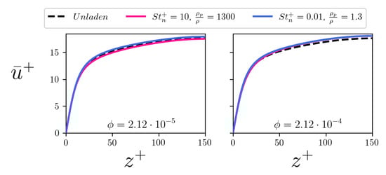
Figure 13.
Mean streamwise fluid velocity along the wall-normal coordinate. The left panel refers to the case, the right panel refers to the case. The curves relative to the fibers are plotted in blue while the curves relative to the fibers are plotted in pink. The curve of the unladen flow case is plotted in dashed black for reference. All cases are normalized according to the shear velocity yield by the corresponding simulation.

Table 1.
Percentage of drag reduction, (defined as in Equation (14)), for the different cases simulated in the (, ) parameter space considered in this study. Drag increase is obtained when , whereas drag reduction is obtained when .
3.4. Root Mean Square Profiles of the Velocities
The profiles of the root mean square (rms) of the fluid velocities allow more insight into the physical mechanism that controls drag modulation. The rms of the streamwise fluid velocity is shown in Figure 14 for all the simulated cases. Tracer-like fibers enhance the rms peak, in agreement with the previous simulations with inertialess spheroids [25]. This rms modulation effect reduces with the volume fraction. Inertial particles, instead, suppress this peak and, at higher , produce a shift of the peak away from the wall.
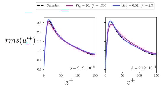
Figure 14.
Root mean square (rms) of the streamwise fluid velocity along the wall-normal coordinate. The left panel refers to the case, the right panel refers to the case. The curves relative to the fibers are plotted in blue while the curves relative to the fibers are plotted in pink. The curve of the unladen flow case is plotted in dashed black for reference. All cases are normalized according to the shear velocity yield by the corresponding simulation.
It can also be observed that all the simulations show a gentle increase of the rms profiles away from the wall. This corresponds to a suppression of turbulent activity and an enlargement of the buffer layer, in qualitative agreement with previous studies on polymer-induced drag reduction [44]. Considering the spanwise rms, shown in Figure 15, tracer-like fibers determine a peak that is located further away from the wall with respect to the unladen case. In addition, at low volume fraction, the mean profile is shifted upwards as one moves away from the wall. This is not observed with the inertial fibers, which appear to shift the profiles downward at increasing volume fraction. Finally, the overall physical picture is coherent also for the wall-normal rms, shown in Figure 16. In this case, all simulations show a gentle reduction, proportional to the volume fraction and to the inertia of the fibers, with the exception of the tracer fibers at low concentration, which seem to slightly detach the profile peak from the wall and increase its value in the center of the channel.
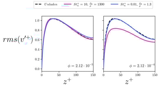
Figure 15.
Root mean square (rms) of the spanwise fluid velocity along the wall-normal coordinate. The left panel refers to the case, the right panel refers to the case. The curves relative to the fibers are plotted in blue while the curves relative to the fibers are plotted in pink. The curve of the unladen flow case is plotted in dashed black for reference.
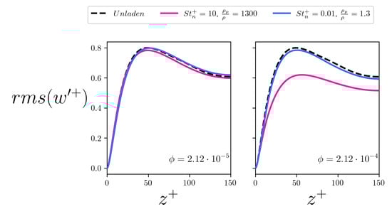
Figure 16.
Root mean square (rms) of the wall-normal fluid velocity along the wall-normal coordinate. The left panel refers to the case, the right panel refers to the case. The curves relative to the fibers are plotted in blue while the curves relative to the fibers are plotted in pink. The curve of the unladen flow case is plotted in dashed black for reference.
3.5. Axial Momentum Balance
In the flow configuration considered in this study, the mean axial momentum balance in the unladen case is determined solely by the viscous shear stress, , and the mixed axial-wall normal Reynolds stress, . The sum of these two contributions provides the total shear stress, , which is a linear function of the wall-normal coordinate [31]:
When a dispersed phase is added to the carrier fluid, an extra stress term must be accounted for in the balance. This extra stress is determined by the presence of the dispersed phase, and is generally referred to as particle extra stress in the following. This term is calculated directly from the two-way coupling force, defined as in Equation (7), in the form of a cumulative integral over a given coordinate :
The momentum balance given by Equation (15) then becomes:
where (simply referred to as hereinafter, for ease of notation). The different contributions to the total balance in the unladen flow case are shown in Figure 17, whereas the contributions in the fiber-laden cases are shown in Figure 18 and Figure 19. Achieving a linear profile for the axial momentum balance is computationally intensive even in the unladen flow case, as statistics need to be calculated on very long averaging windows.
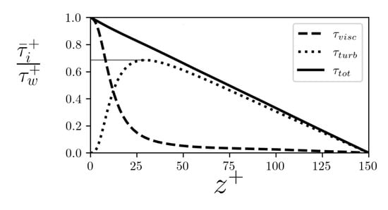
Figure 17.
Unladen-flow momentum balance along the wall-normal coordinate. The viscous shear stress dominates near the wall, while the Reynolds stress takes over away from it. The gray line indicates the maximum value of the Reynolds stress, which is used to compare present results with the fiber-laden ones.
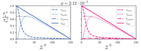
Figure 18.
Axial momentum balance at low volume fraction (). Panels: (left) ; (right) .
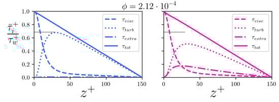
Figure 19.
Axial momentum balance at high volume fraction (). Panels: (left) ; (right) .
Figure 17 demonstrates that our simulations have reached a statistically steady state and ensures that the reported drag reduction is not depending on beneficial but temporary turbulent activity. For the two cases at the lower volume fraction, shown in Figure 18, we can appreciate an effect of the mass loading on the intensity of the fiber extra (axial-normal) stress . This stress is larger for the inertial fibers, while the disturbance given by the tracer-like fibers appears to determine an irrelevant contribution to the momentum balance of the flow (as it is reasonable to expect). At higher volume fraction, as can be seen from Figure 19, the effect of the mass loading is even more clear, as the inertial fibers determine a significant increase of , which qualitatively behaves like a turbulent stress and directly feeds from the Reynolds stress . Finally, we note that, even if the stress determined by the tracer-like fibers has slightly increased with the volume fraction, its contribution to the total momentum balance is still very small.
3.6. Particle Stresses
Equation (16) can be generalized to calculate the mean particle normal stresses, which reveal the non-Newtonian contribution of the dispersed fibers. Fibers introduce a dominant axial-normal stress , that peaks close to the wall before decreasing and vanishing to zero at the center of the channel due to the symmetry of the flow configuration. The intensity of this profile is proportional to the local volume fraction of the dispersed fibers, as one would expect, but also to their inertia. This picture holds for the other non-zero normal stress, , which is shown in Figure 20 and indeed shows a different profile. Starting from the wall, increases up to a distance of about 50 wall units and then maintains an almost constant value in the rest of the channel.
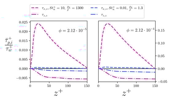
Figure 20.
Particle normal stresses: (left) ; (right) .
Another interesting feature is the fact that, away from the wall, the component is dominated by the component produced by the tracer-like fibers, whereas the situation is the opposite for the inertial cases. Compared with previous studies [25], we can appreciate a difference related to the peak of and , which appear to be less localized than previously observed [25].
4. Conclusions
In this paper, we have presented a statistical characterization of fiber-laden turbulent channel flow in the two-way coupling regime. Statistics refer to almost inertia-less and highly inertial slender fibers whose length extends up to the inertial range of turbulent scales, and were gathered performing highly-resolved Euler–Lagrangian direct numerical simulations and considering four different cases in the Stokes number and fiber volume fraction parameter space. Our study sets itself apart from previous numerical works, as we considered longer particles with a slightly higher aspect ratio but at considerably lower volume fraction [22,23,24,25]. The general picture that emerges from a brief statistical characterization of the laden flows highlights the importance of the volume fraction, which is the key parameter in determining the intensity of the drag reduction. The mass load is also an important parameter as, for inertial fibers, we report a minimal concentration for the onset of drag reduction, below which we have obtained, instead, drag increase. Looking at the turbulence intensities, we appreciate two slightly different behaviors: one efficient case is determined by tracer fibers at low volume fraction, when they determine slightly stronger turbulence intensities, especially for the peak of the axial component and in the bulk of the flow. Instead, the three other simulations highlight a more classical picture, where the turbulence intensities are weakened proportionally with the inertia of the dispersed particles, especially for their peak [44]. Keeping this is mind, we look at the axial momentum balance, where the non-Newtonian, axial-normal particle extra stress appears: from available theories on polymer-induced drag reduction, it is known that this term is limiting the possible amount of drag reduction, therefore it must be considered an undesired effect [44]. At the considered volume fractions, tracer-like fibers do not generate significant extra stresses, while inertial fibers do, feeding from the Reynolds stress proportionally to the mass load. However, tracer-like fibers are capable of introducing a more appreciable normal extra stress, of opposite sign. We speculate here that this stress acts to reduce the axis-wall normal momentum transfer, which can be thought of as the fundamental mechanism on which drag reduction is based [44]. This term, differently from previous studies, shows a profile with non-zero mean all over the channel section and we argue that this is determined by the length of the tracked fibers, which extends well into the inertial range of turbulence at the considered flow Reynolds number [22,23,24,25]. The effectiveness of the tracer-like fibers could be then related to their production of purely normal extra stresses without introducing a relevant particle stress in the momentum balance. Inertial fibers do not exhibit the same feature at lower concentration, as the resulting drag is increased. Instead, at higher volume fraction, the ratio between these two terms becomes more favorable and drag reduction is obtained.
Author Contributions
Conceptualization, C.M.; methodology, D.D.G. and C.M.; software, D.D.G.; validation, D.D.G.; formal analysis, D.D.G. and C.M.; investigation, D.D.G. and C.M.; resources, D.D.G. and C.M.; data curation, D.D.G.; writing D.D.G. and C.M.; writing—review and editing, D.D.G. and C.M.; visualization, D.D.G.; supervision, C.M.; project administration, C.M.; funding acquisition, D.D.G. and C.M. All authors have read and agreed to the published version of the manuscript.
Funding
This research was founded by University of Udine, Doctoral scholarship, XXXV cycle.
Data Availability Statement
Data are contained within the article.
Acknowledgments
The first author acknowledges the Università Italo-Francese, Bando Vinci 2021, cap. 2, progetto C2-257 “Fibre flessibili in flusso turbolento ad elevato numero di Reynolds” for the generous funding. The authors acknowledge the generous allowance of computational ours at CINECA (Iscra B HP10BXAOD6), ALCF (ALCF developer access), and PRACE member Jülich Supercomputing Centre (PRACE PRACE-DEV-2022D01-011).
Conflicts of Interest
The authors declare no conflict of interest. The funders had no role in the design of the study; in the collection, analyses, or interpretation of data; in the writing of the manuscript, or in the decision to publish the results.
Nomenclature
| Drag-reduction percentage | |
| Mean velocity component | |
| Epurated axial pressure gradient | |
| Flow vorticity | |
| Angle between the rigid fiber orientation vector and the velocity gradient direction in a viscous shear flow | |
| Generic particle stress component given by the ith force component over the jth direction | |
| Generic stress component | |
| Length of the turbulent channel flow over th ith direction | |
| Root Mean Square of a variable | |
| Fluctuating velocity component | |
| Identity matrix | |
| Inertia-tensor of any rod element | |
| Shear rate of the viscous shear flow | |
| ℓ | Half-length of any rod element |
| Regularization time-scale of the ERPP method | |
| Aspect ratio of any rod element | |
| Aspect ratio of a full chain of rods | |
| Rod element rotational velocity | |
| Drag Force experienced by the nth rod element of any fiber | |
| Two-way coupling Eulerian force | |
| Hydrodynamic torque on the nth rod element due to the flow velocity gradient | |
| Rod element orientation | |
| Rod element position | |
| Hydrodynamic torque on the nth rod element due to the relative spin between particle and flow | |
| Flow velocity vector at a given Eulerian coordinate | |
| Rod element linear velocity | |
| Eulerian coordinate vector in the absolute frame of reference | |
| Constrain force between the th and the nth rod elements of any fiber | |
| Constrain momentum between the th and the nth rod elements of any fiber | |
| Fluid viscosity | |
| ∇ | Gradient |
| Fluid kinematic viscosity | |
| ∂ | Partial derivative |
| Volume fraction of the fibers | |
| Fluid density | |
| Density of any rod element | |
| Regularization length-scale of the ERPP method | |
| Characteristic response time of the flow at the wall | |
| Response time of any rod element | |
| a | Radius of any rod element |
| Grid spacing in the homogeneous directions | |
| time-step | |
| Maximum grid spacing in the non-homogeneous direction | |
| Minimum grid spacing in the non-homogeneous direction | |
| Young’s Modulus of the rod elements | |
| g | Gaussian function of the ERPP method |
| h | Channel Half-height |
| L | Length of any stretched fiber |
| Mass of any rod element | |
| Number of grid-points in the three coordinates (x,y,z) | |
| Total number of dispersed rods | |
| P | Equivalent pressure gradient |
| Parts Per Million concentration of fibers in weight | |
| Shear Reynolds number | |
| Stokes number | |
| T | Period of a fiber in viscous shear flow |
| t | Time |
| Shear velocity | |
| Volume of the turbulent channel flow | |
| Volume of any rod |
References
- Lundell, F.; Söderberg, L.D.; Alfredsson, P.H. Fluid mechanics of papermaking. Ann. Rev. Fluid Mech. 2011, 43, 195–217. [Google Scholar] [CrossRef]
- Atugoda, T.; Vithanage, M.; Wijesekara, H.; Bolan, N.; Sarmah, A.K.; Bank, M.S.; You, S.; Ok, Y.S. Interactions between microplastics, pharmaceuticals and personal care products: Implications for vector transport. Environ. Int. 2021, 149, 106367. [Google Scholar] [CrossRef] [PubMed]
- Wang, Y.; Zhao, L.; Otto, A.; Robinius, M.; Stolten, D. A review of post-combustion CO2 capture technologies from coal-fired power plants. Energy Procedia 2017, 114, 650–665. [Google Scholar] [CrossRef]
- Campolo, M.; Marchioli, C. Drag Reduction in Turbulent Flows by Polymer and Fiber Additives. KONA Powder Part. J. 2021, 38, 64–81. [Google Scholar]
- Voth, G.A.; Soldati, A. Anisotropic particles in turbulence. Ann. Rev. Fluid Mech. 2017, 49, 249–276. [Google Scholar] [CrossRef]
- Zhao, L.; Marchioli, C.; Andersson, H.I. Slip velocity of rigid fibers in turbulent channel flow. Phys. Fluids 2014, 26, 063302. [Google Scholar] [CrossRef]
- Marchioli, C.; Zhao, L.; Andersson, H.I. On the relative rotational motion between rigid fibers and fluid inturbulent channel flow. Phys. Fluids 2016, 28, 013301. [Google Scholar] [CrossRef]
- Qiu, J.; Marchioli, C.; Andersson, H.I.; Zhao, L. Settling tracer spheroids in vertical turbulent channel flows. Int. J. Multiphase Flow 2019, 118, 173–182. [Google Scholar] [CrossRef]
- Saccone, D.; Marchioli, C.; De Marchis, M. Effect of roughness on elongated particles in turbulent channel flow. Int. J. Multiphase Flow 2022, 152, 104065. [Google Scholar] [CrossRef]
- Forrest, F.; Grierson, G.A. Friction losses in cast iron pipe carrying paper stock. Pap. Trade J. 1931, 92, 39–41. [Google Scholar]
- Toms, B.A. Some observations on the flow of linear polymer solutions through straight tubes at large Reynolds numbers. Proc. First Int. Congr. Rheol. 1948, 2, 135–141. [Google Scholar]
- Wang, Y.; Yu, B.; Zakin, J.L.; Shi, H. Review on drag reduction and its heat transfer by additives. Adv. Mech. Eng. 2011, 3, 478749. [Google Scholar] [CrossRef]
- Metzner, A.B.; Park, M.G. Turbulent flow characteristics of viscoelastic fluids. J. Fluid Mech. 1964, 20, 291–303. [Google Scholar] [CrossRef]
- Gadd, G.E. Turbulence damping and drag reduction produced by certain additives in water. Nature 1965, 206, 463–467. [Google Scholar] [CrossRef]
- Hoyt, J.W. Turbulent Flow of Drag-Reducing Suspensions; National Technical Information Service: Springfield, VA, USA, 1972. [Google Scholar]
- Virk, P.S. Drag Reduction Fundamentals. AIChE J. 1975, 21, 625–656. [Google Scholar] [CrossRef]
- Vaseleski, R.C.; Metzner, A.B. Drag Reduction in the Turbulent Flow of Fiber Suspensions. J. Fluid Mech. 1970, 44, 419–440. [Google Scholar] [CrossRef]
- Radin, I.; Zakin, J.L.; Patterson, G.K. Drag Reduction in Solid-Fluid Systems. AIChE J. 1975, 21, 358–371. [Google Scholar] [CrossRef]
- Lee, P.F.W.; Duffy, G.G. Relationship between velocity profiles and drag reduction in turbulent fiber suspension flow. AIChE J. 1976, 22, 750–753. [Google Scholar] [CrossRef]
- Sharma, R.S. Drag reduction by fibers. Can. J. Chem. Eng. 1981, 59, 3–13. [Google Scholar] [CrossRef]
- Lee, W.K.; Vaseleski, R.C.; Metzner, A.B. Turbulent Drag Reduction in Polymeric Solutions Containing Suspended Fibers. AIChE J. 1974, 20, 128–173. [Google Scholar] [CrossRef]
- Paschkewitz, J.S.; Dubief, Y.; Dimitropoulos, C.D.; Shaqfeh, E.S.; Moin, P. Numerical simulation of turbulent drag reduction using rigid fibers. J. Fluid Mech. 2004, 518, 281–317. [Google Scholar] [CrossRef]
- Gillissen, J.J.J.; Boersma, B.J.; Mortensen, P.H.; Andersson, H.I. Fiber-induced drag reduction. J. Fluid Mech. 2008, 602, 209–218. [Google Scholar] [CrossRef]
- Moosaie, A.; Manhart, M. Direct Monte Carlo simulation of turbulent drag reduction by rigid fibers in a channel flow. Acta Mech. 2013, 224, 2385–2413. [Google Scholar] [CrossRef]
- Wang, Z.; Xu, C.X.; Zhao, L. Turbulence modulations and drag reduction by inertialess spheroids in turbulent channel flow. Phys. Fluids 2021, 33, 123313. [Google Scholar] [CrossRef]
- Gualtieri, P.; Picano, F.; Sardina, G.; Casciola, C. Exact regularized point particle method for multiphase flows in the two-way coupling regime. J. Fluid Mech. 2015, 773, 520–561. [Google Scholar] [CrossRef]
- Dotto, D.; Soldati, A.; Marchioli, C. Deformation of flexible fibers in turbulent channel flow. Meccanica 2019, 55, 343–356. [Google Scholar] [CrossRef]
- Yamamoto, S.; Matsuoka, T. A method for dynamic simulation of rigid and flexible fibers in a flow field. J. Chem. Phys. 1993, 98, 644–650. [Google Scholar] [CrossRef]
- Lindstrom, S.; Uesaka, T. Simulation of the motion of flexible fibers in viscous fluid flow. Phys. Fluids 2007, 98, 644–650. [Google Scholar] [CrossRef]
- Andric, J.; Lindström, S.; Sasic, S. A study of a flexible fiber model and its behavior in DNS of turbulent channel flow. Acta Mech. 2013, 224, 2359–2374. [Google Scholar] [CrossRef]
- Pope, S.B.L. Turbulent Flows; Cambridge University Press: Cambridge, UK, 2000. [Google Scholar]
- Shin, M.; Koch, D.L. Rotational and translational dispersion of fibres in isotropic turbulent flows. J. Fluid Mech. 2005, 540, 143–173. [Google Scholar] [CrossRef]
- Canuto, C.; Hussaini, M.Y.; Quarteroni, A.; Zang, T.A. Spectral Methods; Springer: Berlin, Germany, 2006. [Google Scholar]
- Jeffery, G.B. The Motion of Ellipsoidal Particles Immersed in a Viscous Fluid. Proc. R. Soc. Lond. Ser. A 1922, 1, 161–179. [Google Scholar]
- Cox, R.G. The motion of long slender bodies in a viscous fluid. Part 2. Shear flow. J. Fluid Mech. 1971, 45, 625–657. [Google Scholar] [CrossRef]
- Kim, S.; Karrila, S.J.L. Microhydrodynamics Principles and Selected Applications; Brenner, H., Ed.; Butterworth-Heinemann: Oxford, UK, 1991. [Google Scholar]
- Delmotte, B.; Climent, E.; Plouraboué, F. A general formulation of Bead Models applied to flexible fibers and active filaments at low Reynolds number. J. Comput. Phys. 2015, 286, 14–37. [Google Scholar] [CrossRef]
- Squires, K.D.; Eaton, J.K. Particle response and turbulence modification in isotropic turbulence. Phys. Fluids. 1990, 2, 1191–1203. [Google Scholar] [CrossRef]
- Gillissen, J.J.J.; Boersma, B.J.; Mortensen, P.H.; Andersson, H.I. The stress generated by non-Brownian fibers in turbulent channel flow simulations. Phys. Fluids 2007, 19, 115107. [Google Scholar] [CrossRef]
- Battista, F.; Mollicone, J.; Gualtieri, P.; Messina, R.; Casciola, C. Exact regularised point particle (ERPP) method for particle-laden wall-bounded flows in the two-way coupling regime. J. Fluid Mech. 2019, 878, 420–444. [Google Scholar] [CrossRef]
- Cheng, J.; Grossman, M.; McKercher, T. Professional CUDA C Programming; John Wiley & Sons: Hoboken, NJ, USA, 2014. [Google Scholar]
- Dotto, D.; Marchioli, C. Orientation, distribution, and deformation of inertial flexible fibers in turbulent channel flow. Acta Mech. 2019, 230, 597–621. [Google Scholar] [CrossRef]
- Shaik, S.; Kuperman, S.; Rinsky, V.; van Hout, R. Measurements of length effects on the dynamics of rigid fibers in a turbulent channel flow. Phys. Rev. Fluids 2020, 11, 114309. [Google Scholar] [CrossRef]
- Li, X. Turbulent drag reduction by polymer additives: Fundamentals and recent advances. Phys. Fluids 2019, 31, 121302. [Google Scholar]


Publisher’s Note: MDPI stays neutral with regard to jurisdictional claims in published maps and institutional affiliations. |
© 2022 by the authors. Licensee MDPI, Basel, Switzerland. This article is an open access article distributed under the terms and conditions of the Creative Commons Attribution (CC BY) license (https://creativecommons.org/licenses/by/4.0/).