Internal Energy Relaxation Processes and Bulk Viscosities in Fluids

Abstract

Internal energy relaxation processes in fluid models derived from the kinetic theory are revisited, as are related bulk viscosity coefficients. The apparition of bulk viscosity coefficients in relaxation regimes and the links with equilibrium one-temperature bulk viscosity coefficients are discussed. First, a two-temperature model with a single internal energy mode is investigated, then a two-temperature model with two internal energy modes and finally a state-to-state model for mixtures of gases. All these models lead to a unique physical interpretation of the apparition of bulk viscosity effects when relaxation characteristic times are smaller than fluid times. Monte Carlo numerical simulations of internal energy relaxation processes in model gases are then performed, and power spectrums of density fluctuations are computed. When the energy relaxation time is smaller than the fluid time, both the two temperature and the single-temperature model including bulk viscosity yield a satisfactory description. When the energy relaxation time is larger than the fluid time, however, only the two-temperature model is in agreement with Boltzmann equation. The quantum population of a He-H${}_2$ mixture is also simulated with detailed He-H${}_2$ cross sections, and the resulting bulk viscosity evaluated from the Green–Kubo formula is in agreement with the theory. The impact of bulk viscosity in fluid mechanics is also addressed, as well as various mathematical aspects of internal energy relaxation and Chapman–Enskog asymptotic expansion for a two-temperature fluid model.

1. Introduction

The relaxation of internal energy is of fundamental importance in reentry problems and laboratory plasmas [1,2,3,4,5,6,7,8,9,10,11,12,13,14,15]. Internal energy exchanges notably lead to the apparition of bulk viscosity coefficients in fluid models in relaxation regimes [16,17,18,19,20,21,22,23,24,25,26,27,28]. Theoretical results and experimental measurements have further shown that bulk viscosity coefficients of polyatomic gases are of the order of shear viscosity coefficients [29,30,31,32,33,34,35]. These are strong motivations for investigating internal energy relaxation processes and related bulk viscosity coefficients in nonequilibrium models derived from the kinetic theory of gases.

A hierarchy of thermodynamic nonequilibrium fluid models may be derived from the kinetic theory of polyatomic gas mixtures. The most general thermodynamic nonequilibrium model is the state-to-state model, in which each internal state of a molecule is independent and considered as a separate species [1,2,3,4,5,6,7,8,9,10,11,12,13]. When the internal states are lumped into energy bins, coarse-grained models are obtained, with each bin considered a separate species [14,15]. When there are partial equilibria between some of the bins or between the internal states, species internal energy temperatures may be defined, and the complexity of the model is reduced accordingly [9]. The next reduction step consists of equating some of the species’ internal temperatures with the equilibrium one-temperature model ultimately obtained [9]. Each relaxation step towards a simpler and more equilibrated model then yields bulk viscosity contributions—provided the characteristic energy relaxation times are smaller than the flow times, the most complete bulk viscosity coefficient being that obtained for the equilibrium one-temperature fluid [26,27,28].

A simplified kinetic model where elastic and resonant collisions are fast but collisions exchanging translational and internal energy are slow is first considered [26]. In such a framework, the translational and internal temperatures are macroscopic quantities associated with collisional invariants of the fast collision operator. In a relaxation regime, when the characteristic time of internal energy relaxation is smaller than the flow characteristic time, the difference between the translational temperature $T^{\mathrm{tr}}$ and the equilibrium temperature T becomes proportional to the divergence of the velocity field $\mathit{v}$. This leads to the apparition of a bulk viscosity coefficient $\kappa$, such that $n{k}_{\mathrm{B}}(T^{\mathrm{tr}}-T)=-\kappa \mathbf{\nabla }·\mathit{v}$ where n is the number density and $k_{\mathrm{B}}$ the Boltzmann constant.

A more complex situation with two internal energy modes, one with a slow exchange rate and the other one with a fast exchange rate, is then investigated [26]. The translational-rapid mode temperature and the slow mode temperature are then collisional invariants of the fast collision operator. For such a model, there is a bulk viscosity due to the fast internal energy mode, as in classical one-temperature models, but part of the thermodynamic equilibrium bulk viscosity is still hidden in the slow internal mode. A detailed analysis yields that, in a relaxation regime, there are five contributions to the effective bulk viscosity, namely the fast internal mode bulk viscosity, the slow internal mode bulk viscosity, the reduced relaxation pressure and two perturbed relaxation source terms. In the thermodynamic equilibrium limit, the sum of these five contributions coincide with the one-temperature two-mode bulk viscosity. The physical interpretation of the origin of the bulk viscosity coefficient is found to be similar to that of the simplified two-temperature model [26]. This analysis may also be generalized to the situation of gas mixtures, as well as to the case of nonindependent energy modes [27].

Next, the general situation of state-to-state mixture models in which each quantum state of each species is independent is considered [28]. Relaxation equations in symmetric form are derived for the quantum state population Gibbs functions and the translational temperature. Approximate solutions of the population relaxation equations compatible with the asymptotic equilibrium limit are then obtained. At zeroth order, using a relaxation approximation, the differences between the pseudo species’ chemical potentials and their equilibrium value are proportional to the divergence of the velocity field. The ‘internal energy’ bulk viscosity ${\kappa }_{\left[01\right]}$ is then recovered with the relation $n{k}_{\mathrm{B}}(T^{\mathrm{tr}}-T)=-{\kappa }_{\left[01\right]}\mathbf{\nabla }·\mathit{v}$. At first order, the relaxation approximation yields a bulk viscosity that converges at thermodynamic equilibrium towards the traditional bulk viscosity.

Monte Carlo simulations of spontaneous fluctuations near thermodynamic equilibrium are then performed in order to investigate a polyatomic model gas [36,37,38]. The density fluctuation power spectrum of the model gas is evaluated by using the Boltzmann equation, as well as linearized fluid equations [7,26,39,40,41,42]. The simplified one-temperature model, including the bulk viscosity term, then well agrees with Boltzmann equation when the internal energy relaxation time is smaller than the flow time [26,27]. When the relaxation time is larger than the flow characteristic time, however, only the two-temperature model is in agreement with Boltzmann equation.

Next, a state-to-state model for mixtures of Helium and Hydrogen is investigated numerically. The required collision integrals are evaluated from a complete set of state-to-state cross sections for the $\mathrm{He}+{\mathrm{H}}_2(v,\mathrm{J})$ collisional system. The latter have been obtained using an implementation of the quasiclassical method [43,44,45,46,47] with the accurate Muchnik–Russek potential energy surface [48,49,50,51,52,53,54,55,56]. The values of the bulk viscosity for the model gas, obtained from the fluctuation–dissipation theory [57,58,59,60,61,62,63,64,65,66,67,68,69], are then in full agreement with the theory [28].

The impact of bulk viscosity in fluid mechanics, which has scarcely been discussed in the literature [70,71,72,73,74,75,76,77], is further addressed. The success of the erroneous Stokes approximation is mostly due to the gradient structure of the bulk viscosity term [74]. The mathematical structure of relaxation systems of partial differential equations and their symmetry is also discussed [78,79,80,81,82,83,84,85,86,87,88,89,90,91,92,93,94,95,96,97]. Various mathematical aspects associated with the Chapman–Enskog method for partial-differential equations are also addressed and applied to the simplified two-temperature model, and found to agree with formal expansions [82,94,95,96,97].

The simplified two-temperature model is considered in Section 2, the two-temperature two-mode nonequilibrium model in Section 3, and the state-to-state model in Section 4. The Monte Carlo simulations of single gases are presented in Section 5 and that of state-to-state mixture models in Section 6. The impact in fluid mechanics and the mathematical aspects are finally addressed in Section 7.

2. A Simplified Two-Temperature Model

2.1. Kinetic Framework

A single polyatomic gas is considered with the Boltzmann equation written in the form

$${\partial }_t^{}f+\mathit{c}·\mathbf{\nabla }f=\frac{1}{ϵ}{\mathcal{J}}^{\mathrm{rap}}+{\mathcal{J}}^{\mathrm{sl}},$$

(1)

where ${\partial }_t^{}$ denotes the time derivative operator, $\mathit{c}$ the particle velocity, ∇ the space derivative operator, $f(t,\mathit{x},\mathit{c},\mathrm{I})$ the distribution function, $\mathit{x}$ the spatial coordinate, I the index of the quantum energy state, ${\mathcal{J}}^{\mathrm{rap}}$ the rapid collision operator, ${\mathcal{J}}^{\mathrm{sl}}$ the slow collision operator, and $ϵ$ the formal parameter associated with the Chapman–Enskog procedure. The complete collision operator $\mathcal{J}={\mathcal{J}}^{\mathrm{rap}}+{\mathcal{J}}^{\mathrm{sl}}$ is in the form

$$\mathcal{J}\left(f\right)=\sum _{\mathrm{J},{\mathrm{I}}^{\prime },{\mathrm{J}}^{\prime }}\int \left(f({\mathit{c}}^{\prime },{\mathrm{I}}^{\prime })f({\tilde{\mathit{c}}}^{\prime },{\mathrm{J}}^{\prime })\frac{a_{\mathrm{I}}{a}_{\mathrm{J}}}{a_{{\mathrm{I}}^{\prime }}{a}_{{\mathrm{J}}^{\prime }}}-f(\mathit{c},\mathrm{I})f(\tilde{\mathit{c}},\mathrm{J})\right)g{\sigma }^{\mathrm{I}\mathrm{J}{\mathrm{I}}^{\prime }{\mathrm{J}}^{\prime }}\mathrm{d}\tilde{\mathit{c}}\mathrm{d}{\mathit{e}}^{\prime },$$

(2)

where in a direct collision i and j denote the indices of the quantum energy states before collision, ${\mathrm{I}}^{\prime }$ and ${\mathrm{J}}^{\prime }$ the corresponding numbers after collision, $\tilde{\mathit{c}}$ the velocity of the colliding partner, ${\mathit{c}}^{\prime }$ and ${\tilde{\mathit{c}}}^{\prime }$ the velocities after collision, $a_{\mathrm{I}}$ the degeneracy of the ith quantum energy state, g the absolute value of the relative velocity $\mathit{c}-\tilde{\mathit{c}}$, ${\mathit{e}}^{\prime }$ the unit vector in the direction of the relative velocity ${\mathit{c}}^{\prime }-{\tilde{\mathit{c}}}^{\prime }$, and ${\sigma }^{\mathrm{I}\mathrm{J}{\mathrm{I}}^{\prime }{\mathrm{J}}^{\prime }}$ the collision cross sections [18,22]. The dependence of f on $(t,\mathit{x})$ has been left implicit in (2) and the cross sections ${\sigma }^{\mathrm{I}\mathrm{J}{\mathrm{I}}^{\prime }{\mathrm{J}}^{\prime }}$ satisfy the reciprocity relations $a_{\mathrm{I}}{a}_{\mathrm{J}}g{\sigma }^{\mathrm{I}\mathrm{J}{\mathrm{I}}^{\prime }{\mathrm{J}}^{\prime }}\mathrm{d}\mathit{c}\mathrm{d}\tilde{\mathit{c}}\mathrm{d}{\mathit{e}}^{\prime }=a_{{\mathrm{I}}^{\prime }}{a}_{{\mathrm{J}}^{\prime }}{g}^{\prime }{\sigma }^{{\mathrm{I}}^{\prime }{\mathrm{J}}^{\prime }\mathrm{I}\mathrm{J}}\mathrm{d}{\mathit{c}}^{\prime }\mathrm{d}{\tilde{\mathit{c}}}^{\prime }\mathrm{d}\mathit{e}$.

Denoting by $E_{\mathrm{I}}$ the internal energy in the ith state, the rapid collisions are either elastic without change of internal energy or resonant with $\Delta E=E_{{\mathrm{I}}^{\prime }}+E_{{\mathrm{J}}^{\prime }}-E_{\mathrm{I}}-E_{\mathrm{J}}=0$, $E_{{\mathrm{I}}^{\prime }}\ne E_{\mathrm{I}}$ and $E_{{\mathrm{J}}^{\prime }}\ne E_{\mathrm{J}}$, whereas the slow collisions are such that $\Delta E=E_{{\mathrm{I}}^{\prime }}+E_{{\mathrm{J}}^{\prime }}-E_{\mathrm{I}}-E_{\mathrm{J}}\ne 0$. Denoting by ${\mathcal{J}}^{\mathrm{tr}-\mathrm{tr}}$ the operator associated with elastic collision, ${\mathcal{J}}^{\mathrm{int}-\mathrm{int}}$ the operator associated with resonant collisions, and ${\mathcal{J}}^{\mathrm{tr}-\mathrm{int}}$ the operator associated with collisions, such that $\Delta E\ne 0$, the fast and slow collision operators are then

$${\mathcal{J}}^{\mathrm{rap}}={\mathcal{J}}^{\mathrm{tr}-\mathrm{tr}}+{\mathcal{J}}^{\mathrm{int}-\mathrm{int}},{\mathcal{J}}^{\mathrm{sl}}={\mathcal{J}}^{\mathrm{tr}-\mathrm{int}}.$$

(3)

The collisional invariants of the fast collision operator ${\mathcal{J}}^{\mathrm{rap}}$ are associated with particle number ${\psi }^1=1$, momentum ${\psi }^{1+\nu }=m{c}_{\nu }$, $\nu \in \{1,2,3\}$ with $\mathit{c}={(c_1,c_2,c_3)}^t$, kinetic energy ${\psi }^5={\psi }^{\mathrm{tr}}=\frac{1}{2}m{|\mathit{c}-\mathit{v}|}^2$ and internal energy ${\psi }^6={\psi }^{\mathrm{int}}=E_{\mathrm{I}}$ where m denotes the particle mass and $\mathit{v}$ the fluid velocity.

The Enskog expansion is in the form $f=f^{\left(0\right)}\left(1+ϵ\varphi +\mathcal{O}\left({ϵ}^2\right)\right)$ and the Maxwellian distribution $f^{\left(0\right)}$ reads

$$f^{\left(0\right)}={\left(\frac{m}{2\pi k_{\mathrm{B}}{T}^{\mathrm{tr}}}\right)}^{\frac{3}{2}}\frac{n{a}_{\mathrm{I}}}{Z^{\mathrm{int}}}exp\left(-\frac{{m|\mathit{c}-\mathit{v}|}^2}{2k_{\mathrm{B}}{T}^{\mathrm{tr}}}-\frac{E_{\mathrm{I}}}{k_{\mathrm{B}}{T}^{\mathrm{int}}}\right),$$

(4)

where n denotes the number density, $k_{\mathrm{B}}$ the Boltzmann constant, $T^{\mathrm{tr}}$ the translational temperature, $T^{\mathrm{int}}$ the internal temperature, and $Z^{\mathrm{int}}={\sum }_{\mathrm{I}}{a}_{\mathrm{I}}exp\left(-E_{\mathrm{I}}/k_{\mathrm{B}}{T}^{\mathrm{int}}\right)$ the partition function. There are two different temperatures, $T^{\mathrm{tr}}$ and $T^{\mathrm{int}}$, in $f^{\left(0\right)}$, since there are two different energy collisional invariants: ${\psi }^{\mathrm{tr}}$ and ${\psi }^{\mathrm{int}}$. The scalar product $⟨⟨\xi ,\zeta ⟩⟩$ between two tensorial quantities $\xi (t,\mathit{x},\mathit{c},\mathrm{I})$ and $\zeta (t,\mathit{x},\mathit{c},\mathrm{I})$ is naturally defined by

$$⟨⟨\xi ,\zeta ⟩⟩=\sum _{\mathrm{I}}\int \xi ·\zeta \mathrm{d}\mathit{c}.$$

where $\xi ·\zeta$ is the contracted product.

The equations for conservation of mass, momentum and internal energies are then obtained by taking the scalar product of the Boltzmann equation (1) with the collisional invariants of the fast collision operator. The corresponding fluid variables are the particle number density $n=⟨⟨{\psi }^1,f⟩⟩=⟨⟨{\psi }^1,f^{\left(0\right)}⟩⟩$ or, equivalently, the mass density $\rho =mn$, the mass averaged velocity $\mathit{v}$ with $\rho \mathit{v}=⟨⟨m\mathit{c},f⟩⟩=⟨⟨m\mathit{c},f^{\left(0\right)}⟩⟩$, the internal energy per unit volume of translational origin ${\mathcal{E}}^{\mathrm{tr}}=⟨⟨f,{\psi }^{\mathrm{tr}}⟩⟩=⟨⟨f^{\left(0\right)},{\psi }^{\mathrm{tr}}⟩⟩$, and the internal energy per unit volume of internal origin ${\mathcal{E}}^{\mathrm{int}}=⟨⟨f,{\psi }^{\mathrm{int}}⟩⟩=⟨⟨f^{\left(0\right)},{\psi }^{\mathrm{int}}⟩⟩$, or, equivalently, the translation and internal temperatures $T^{\mathrm{tr}}$ and $T^{\mathrm{int}}$ defined by ${\mathcal{E}}^{\mathrm{tr}}(T^{\mathrm{tr}},n)=⟨⟨f,{\psi }^{\mathrm{tr}}⟩⟩$ and ${\mathcal{E}}^{\mathrm{int}}(T^{\mathrm{int}},n)=⟨⟨f,{\psi }^{\mathrm{int}}⟩⟩$. The pressure p and the internal energies ${\mathcal{E}}^{\mathrm{tr}}$ and ${\mathcal{E}}^{\mathrm{int}}$ are found in the form

$$p=n{k}_{\mathrm{B}}{T}^{\mathrm{tr}},{\mathcal{E}}^{\mathrm{tr}}=n\frac{3}{2}{k}_{\mathrm{B}}{T}^{\mathrm{tr}},{\mathcal{E}}^{\mathrm{int}}=n\overline{E},$$

(5)

where $\overline{E}={\sum }_{\mathrm{I}}\frac{a_{\mathrm{I}}{E}_{\mathrm{I}}}{Z^{\mathrm{int}}}exp\left(-E_{\mathrm{I}}/k_{\mathrm{B}}{T}^{\mathrm{int}}\right)$ is the average internal energy per particle. The corresponding translational and internal entropies and Gibbs functions are presented in [26]. Following the Chapman–Enskog procedure, the equations for conservation of mass, momentum, and internal energies are obtained in the form [9]

$$\begin{array}{cc}\hfill & {\partial }_t^{}\rho +\mathbf{\nabla }·\left(\rho \mathit{v}\right)=0,\hfill \end{array}$$

(6)

$$\begin{array}{cc}\hfill & {\partial }_t^{}\left(\rho \mathit{v}\right)+\mathbf{\nabla }·(\rho \mathit{v}\otimes \mathit{v}+p\mathit{I})+\mathbf{\nabla }·\mathit{\Pi }=0,\hfill \end{array}$$

(7)

$$\begin{array}{cc}\hfill & {\partial }_t{\mathcal{E}}^{\mathrm{tr}}+\mathbf{\nabla }·\left(\mathit{v}{\mathcal{E}}^{\mathrm{tr}}\right)+\mathbf{\nabla }·{\mathit{Q}}^{\mathrm{tr}}=-p\mathbf{\nabla }·\mathit{v}-\mathit{\Pi }:\mathbf{\nabla }\mathit{v}-{\omega }_1^{\mathrm{int}},\hfill \end{array}$$

(8)

$$\begin{array}{cc}\hfill & {\partial }_t{\mathcal{E}}^{\mathrm{int}}+\mathbf{\nabla }·\left(\mathit{v}{\mathcal{E}}^{\mathrm{int}}\right)+\mathbf{\nabla }·{\mathit{Q}}^{\mathrm{int}}={\omega }_1^{\mathrm{int}},\hfill \end{array}$$

(9)

where ⊗ denotes the tensor vector product, $\mathit{I}$ the unit tensor, $\mathit{\Pi }$ the viscous tensor, ${\mathit{Q}}^{\mathrm{tr}}$ the translational energy heat flux, ${\mathit{Q}}^{\mathrm{int}}$ the internal energy heat flux and ${\omega }_1^{\mathrm{int}}$ the first-order energy exchange term. The transport fluxes are given by

$$\begin{array}{cc}\hfill \mathit{\Pi }=& -\eta \left(\mathbf{\nabla }\mathit{v}+{(\mathbf{\nabla }\mathit{v})}^t-\frac{2}{3}(\mathbf{\nabla }·\mathit{v})\mathit{I}\right),\hfill \end{array}$$

(10)

$$\begin{array}{cc}\hfill {\mathit{Q}}^{\mathrm{tr}}=& -{\lambda }^{\mathrm{tr},\mathrm{tr}}\mathbf{\nabla }{T}^{\mathrm{tr}}-{\lambda }^{\mathrm{tr},\mathrm{int}}\mathbf{\nabla }{T}^{\mathrm{int}},\hfill \end{array}$$

(11)

$$\begin{array}{cc}\hfill {\mathit{Q}}^{\mathrm{int}}=& -{\lambda }^{\mathrm{int},\mathrm{tr}}\mathbf{\nabla }{T}^{\mathrm{tr}}-{\lambda }^{\mathrm{int},\mathrm{int}}\mathbf{\nabla }{T}^{\mathrm{int}},\hfill \end{array}$$

(12)

where $\eta$ denotes the shear viscosity, and ${\lambda }^{\mathrm{tr},\mathrm{tr}}$, ${\lambda }^{\mathrm{tr},\mathrm{int}}$, ${\lambda }^{\mathrm{int},\mathrm{tr}}$, and ${\lambda }^{\mathrm{int},\mathrm{int}}$ the thermal conductivities. The full source term ${\omega }^{\mathrm{int}}=⟨⟨{\psi }^{\mathrm{int}},{\mathcal{J}}^{\mathrm{sl}}⟩⟩=⟨⟨{\psi }^{\mathrm{int}},\mathcal{J}⟩⟩$ may be expanded as ${\omega }^{\mathrm{int}}={\omega }_0^{\mathrm{int}}+ϵ\delta {\omega }_1^{\mathrm{int}}+\mathcal{O}\left({ϵ}^2\right)$ where ${\omega }_0^{\mathrm{int}}$ is evaluated from the Maxwellian distribution $f^{\left(0\right)}$ and $\delta {\omega }_1^{\mathrm{int}}$ is the correction associated with the Navier–Stokes perturbation $\varphi$, so that the first-order source term ${\omega }_1^{\mathrm{int}}$ is given by

$${\omega }_1^{\mathrm{int}}={\omega }_0^{\mathrm{int}}+ϵ\delta {\omega }_1^{\mathrm{int}}.$$

(13)

Finally, the pressure tensor $\mathcal{P}=p\mathit{I}+\mathit{\Pi }$ is given by

$$\mathcal{P}=n{k}_{\mathrm{B}}{T}^{\mathrm{tr}}\mathit{I}-\eta \left(\mathbf{\nabla }\mathit{v}+{(\mathbf{\nabla }\mathit{v})}^t-\frac{2}{3}(\mathbf{\nabla }·\mathit{v})\mathit{I}\right),$$

(14)

and does not involve a bulk viscosity term, unlike one-temperature polyatomic gas models [16,17,18,19,20,21,22,23,24,25].

2.2. Relaxation and Bulk Viscosity

From the energy Equations (8) and (9) it is obtained at zeroth order that

$${\partial }_t{T}^{\mathrm{tr}}+\mathit{v}·\mathbf{\nabla }{T}^{\mathrm{tr}}=-\frac{p\mathbf{\nabla }·\mathit{v}}{n{c}^{\mathrm{tr}}}-\frac{{\omega }_0^{\mathrm{int}}}{n{c}^{\mathrm{tr}}},{\partial }_t{T}^{\mathrm{int}}+\mathit{v}·\mathbf{\nabla }{T}^{\mathrm{int}}=\frac{{\omega }_0^{\mathrm{int}}}{n{c}^{\mathrm{int}}},$$

(15)

where the heat capacities are given by

$$c^{\mathrm{tr}}=\frac{3}{2}{k}_{\mathrm{B}},c^{\mathrm{int}}=\sum _{\mathrm{I}}\frac{k_{\mathrm{B}}{a}_{\mathrm{I}}}{Z^{\mathrm{int}}}{\left(\frac{E_{\mathrm{I}}-\overline{E}}{k_{\mathrm{B}}{T}^{\mathrm{int}}}\right)}^{2}exp\left(-\frac{E_{\mathrm{I}}}{k_{\mathrm{B}}{T}^{\mathrm{int}}}\right),c^{\mathrm{vl}}=c^{\mathrm{tr}}+c^{\mathrm{int}}.$$

The zeroth-order source term ${\omega }_0^{\mathrm{int}}$ is in the form ${\omega }_0^{\mathrm{int}}=-2n^2\left[\left[(\Delta E)\left(exp\left(\frac{\Delta E}{k_{\mathrm{B}}{T}^{\mathrm{tr}}}-\frac{\Delta E}{k_{\mathrm{B}}{T}^{\mathrm{int}}}\right)-1\right)\right]\right]$ where $\left[\right[\left]\right]$ is the averaging operator $\left[\right[\alpha \left]\right]=\frac{1}{8n^2}{\sum }_{\mathrm{I},\mathrm{J},{\mathrm{I}}^{\prime },{\mathrm{J}}^{\prime }}\int {\alpha }_{\mathrm{I}\mathrm{J}{\mathrm{I}}^{\prime }{\mathrm{J}}^{\prime }}{f}^{\left(0\right)}{\tilde{f}}^{\left(0\right)}g{\sigma }^{\mathrm{I}\mathrm{J}{\mathrm{I}}^{\prime }{\mathrm{J}}^{\prime }}\mathrm{d}\mathit{c}\mathrm{d}\tilde{\mathit{c}}\mathrm{d}{\mathit{e}}^{\prime }$. Defining the nonequilibrium correction factor by $\zeta ={\int }_0^{1}exp\left((\frac{\Delta E}{k_{\mathrm{B}}{T}^{\mathrm{tr}}}-\frac{\Delta E}{k_{\mathrm{B}}{T}^{\mathrm{int}}})s\right)ds$ and the relaxation time by ${\tau }^{\mathrm{int}}=c^{\mathrm{int}}{k}_{\mathrm{B}}{T}^{\mathrm{tr}}{T}^{\mathrm{int}}/2n\left[\left[{(\Delta E)}^2\zeta \right]\right]$, the source term ${\omega }_0^{\mathrm{int}}$ may be rewritten in the relaxation form

$${\omega }_0^{\mathrm{int}}=\frac{n{c}^{\mathrm{int}}}{{\tau }^{\mathrm{int}}}(T^{\mathrm{tr}}-T^{\mathrm{int}}).$$

(16)

Subtracting the $T^{\mathrm{int}}$ equation from that for $T^{\mathrm{tr}}$ and using (16), the resulting equation for $T^{\mathrm{tr}}-T^{\mathrm{int}}$ reads

$${\partial }_t(T^{\mathrm{tr}}-T^{\mathrm{int}})+\mathit{v}·\mathbf{\nabla }(T^{\mathrm{tr}}-T^{\mathrm{int}})=-\frac{p\mathbf{\nabla }·\mathit{v}}{n{c}^{\mathrm{tr}}}-\frac{c^{\mathrm{vl}}}{c^{\mathrm{tr}}}\frac{T^{\mathrm{tr}}-T^{\mathrm{int}}}{{\tau }^{\mathrm{int}}}.$$

(17)

This is a typical relaxation equation, and when ${\tau }^{\mathrm{int}}$ is smaller that the flow characteristic time, the relaxation relation $T^{\mathrm{tr}}-T^{\mathrm{int}}=-{\tau }^{\mathrm{int}}p\mathbf{\nabla }·\mathit{v}/n{c}^{\mathrm{vl}}$ is obtained after some initial layer. The equilibrium temperature is naturally defined as the unique scalar T, such that

$${\mathcal{E}}^{\mathrm{tr}}\left(T\right)+{\mathcal{E}}^{\mathrm{int}}\left(T\right)={\mathcal{E}}^{\mathrm{tr}}\left(T^{\mathrm{tr}}\right)+{\mathcal{E}}^{\mathrm{int}}\left(T^{\mathrm{int}}\right),$$

(18)

and only this temperature T is available for the limiting one-temperature fluid model. Letting ${\tilde{c}}^{\mathrm{int}}={\int }_0^1{c}^{\mathrm{int}}\left(T^{\mathrm{int}}+s(T-T^{\mathrm{int}})\right)\mathrm{d}s$, we then have ${\mathcal{E}}^{\mathrm{int}}\left(T\right)-{\mathcal{E}}^{\mathrm{int}}\left(T^{\mathrm{int}}\right)={\tilde{c}}^{\mathrm{int}}(T-T^{\mathrm{int}})$ and $c^{\mathrm{tr}}(T^{\mathrm{tr}}-T)={\tilde{c}}^{\mathrm{int}}(T-T^{\mathrm{int}})$. The bulk viscosity is also defined by $\kappa =p{k}_{\mathrm{B}}{\tilde{c}}^{\mathrm{int}}{\tau }^{\mathrm{int}}/c^{\mathrm{vl}}{\tilde{c}}^{\mathrm{vl}}$ where ${\tilde{c}}^{\mathrm{vl}}=c^{\mathrm{tr}}+{\tilde{c}}^{\mathrm{int}}$ so that

$$\kappa =\frac{c^{\mathrm{int}}{\tilde{c}}^{\mathrm{int}}}{c^{\mathrm{vl}}{\tilde{c}}^{\mathrm{vl}}}\frac{k_{\mathrm{B}}^3{\left(T^{\mathrm{tr}}\right)}^2{T}^{\mathrm{int}}}{2\left[\left[{(\Delta E)}^2\zeta \right]\right]},$$

(19)

and the equilibrium limit of this coefficient is ${\left(\frac{c^{\mathrm{int}}}{c^{\mathrm{vl}}}\right)}^2{\left(k_{\mathrm{B}}T\right)}^3/2\left[\left[{(\Delta E)}^2\right]\right]$, which coincides with the bulk viscosity coefficient obtained independently from the Chapman–Enskog method for the equilibrium fluid [34,35]. Combining the relaxation relation with $c^{\mathrm{tr}}(T^{\mathrm{tr}}-T)={\tilde{c}}^{\mathrm{int}}(T-T^{\mathrm{int}})$ and the definition of $\kappa$, we obtain the fundamental relation

$$n{k}_{\mathrm{B}}(T^{\mathrm{tr}}-T)=-\kappa \mathbf{\nabla }·\mathit{v}.$$

(20)

The pressure tensor $\mathcal{P}$ is then in the form

$$\mathcal{P}=n{k}_{\mathrm{B}}T\mathit{I}-\kappa \mathbf{\nabla }·\mathit{v}\mathit{I}-\eta \left(\mathbf{\nabla }\mathit{v}+{(\mathbf{\nabla }\mathit{v})}^t-\frac{2}{3}(\mathbf{\nabla }·\mathit{v})\mathit{I}\right),$$

(21)

and the bulk viscosity coefficient of the one-temperature equilibrium limit fluid that only involves T has been recovered. Many authors have discussed the near thermodynamic equilibrium situation, where the internal temperature $T^{\mathrm{int}}$ and the translational temperature $T^{\mathrm{tr}}$ are a priori close; notably, Kohler [16], Hirschfelder Curtiss and Bird [17], Waldmann [18], Chapman and Cowling [19], Ferziger and Kapper [20], McCourt et al. [21], de Groot and Mazur [24], Keizer [25], Zhdanov [8], Nagnibeda and Kustova [9] and Brun [10].

It is also possible to establish that first-order corrections to the bulk viscosity coefficient are negligible for such a simplified two-temperature model. Discarding Burnett-type terms, the corrections indeed involve the perturbed source term $\delta {\omega }_1^{\mathrm{int}}$ that is in the form $\delta {\omega }_1^{\mathrm{int}}=⟨⟨f^{\left(0\right)}\varphi ,{\mathcal{W}}^{\mathrm{int}}⟩⟩=⟨⟨f^{\left(0\right)}{\varphi }^{\omega },{\mathcal{W}}^{\mathrm{int}}⟩⟩{\omega }_0^{\mathrm{int}}$ where ${\varphi }^{\omega }$ is the scalar perturbed distribution function arising from the expansion [26]

$$\varphi =-{\varphi }^{\eta }:\mathbf{\nabla }\mathit{v}-{\varphi }^{{\lambda }^{\mathrm{tr}}}·\mathbf{\nabla }\left(\frac{1}{k_{\mathrm{B}}{T}^{\mathrm{tr}}}\right)-{\varphi }^{{\lambda }^{\mathrm{int}}}·\mathbf{\nabla }\left(\frac{1}{k_{\mathrm{B}}{T}^{\mathrm{int}}}\right)+{\varphi }^{\omega }{\omega }_0^{\mathrm{int}},$$

with ${\varphi }^{\eta }$ denoting a symmetric traceless tensor; ${\varphi }^{{\lambda }^{\mathrm{tr}}}$ and ${\varphi }^{{\lambda }^{\mathrm{int}}}$ are vectors [9,26]. However, the standard scalar basis functions ${\varphi }^{0010}=\frac{3}{2}-\frac{1}{2}\frac{m}{k_{\mathrm{B}}T}{|\mathit{c}-\mathit{v}|}^2$ and ${\varphi }^{0001}=(\overline{E}-E_{\mathrm{I}})/k_{\mathrm{B}}{T}^{\mathrm{int}}$ used for scalar linearized kinetic equations are both collisional invariants of the rapid collision operator, and are therefore in the nullspace of the linearized fast collision operator ${\mathcal{I}}^{\mathrm{rap}}$. Therefore, the perturbed term vanishes ${\varphi }^{\omega }\simeq 0$ in a first approximation, so that ${\omega }_1^{\mathrm{int}}\simeq {\omega }_0^{\mathrm{int}}$, and there are no first-order corrections to the bulk viscosity coefficient [26].

3. A Two-Mode Two-Temperature Model

3.1. Kinetic Framework

A single polyatomic gas with two independent internal energy modes that have different exchange rates is now considered. The first mode is assumed to have a rapid exchange rate with the translational degrees of freedom, whereas the other one is assumed to have a slow exchange rate. The internal energy in the ith quantum state is accordingly split as

$$E_{\mathrm{I}}=E_{{\mathrm{I}}^{\mathrm{rap}}}^{\mathrm{rap}}+E_{{\mathrm{I}}^{\mathrm{sl}}}^{\mathrm{sl}},$$

(22)

where I denotes the composed index $\mathrm{I}=({\mathrm{I}}^{\mathrm{rap}},{\mathrm{I}}^{\mathrm{sl}})$, ${\mathrm{I}}^{\mathrm{rap}}$ the index of the quantum energy state of the rapid mode, ${\mathrm{I}}^{\mathrm{sl}}$ the index of the quantum energy state of the slow mode, $E_{{\mathrm{I}}^{\mathrm{rap}}}^{\mathrm{rap}}$ the rapid mode internal energy, and $E_{{\mathrm{I}}^{\mathrm{sl}}}^{\mathrm{sl}}$ the slow mode internal energy. It is denoted for short $E_{\mathrm{I}}^{\mathrm{rap}}$ for $E_{{\mathrm{I}}^{\mathrm{rap}}}^{\mathrm{rap}}$ and $E_{\mathrm{I}}^{\mathrm{sl}}$ for $E_{{\mathrm{I}}^{\mathrm{sl}}}^{\mathrm{sl}}$, so that $E_{\mathrm{I}}=E_{\mathrm{I}}^{\mathrm{rap}}+E_{\mathrm{I}}^{\mathrm{sl}}$. The degeneracy of the Ith state is also denoted by $a_{\mathrm{I}}$ and may be decomposed as $a_{\mathrm{I}}=a_{{\mathrm{I}}^{\mathrm{rap}}}^{\mathrm{rap}}{a}_{{\mathrm{I}}^{\mathrm{sl}}}^{\mathrm{sl}}$ where $a_{{\mathrm{I}}^{\mathrm{rap}}}^{\mathrm{rap}}$ and $a_{{\mathrm{I}}^{\mathrm{sl}}}^{\mathrm{sl}}$ are the degeneracies of the fast and slow modes. The rapid collisions are all collisions, such that $\Delta E^{\mathrm{sl}}=E_{{\mathrm{I}}^{\prime }}^{\mathrm{sl}}+E_{{\mathrm{J}}^{\prime }}^{\mathrm{sl}}-E_{\mathrm{I}}^{\mathrm{sl}}-E_{\mathrm{J}}^{\mathrm{sl}}=0$, either only involving the translational and rapid mode energy or resonant with respect to the slow internal mode. Denoting by ${\mathcal{J}}^{(\mathrm{tr}+\mathrm{rap})-(\mathrm{tr}+\mathrm{rap})}$ the collision operator involving solely the translational and fast internal degrees of freedom, ${\mathcal{J}}^{\mathrm{sl}-\mathrm{sl}}$ the operator for resonant collision with respect to $E^{\mathrm{sl}}$, and ${\mathcal{J}}^{(\mathrm{tr}+\mathrm{rap})-\mathrm{sl}}$ the operator for collisions, such that $\Delta E^{\mathrm{sl}}\ne 0$, the Boltzmann equation governing the distribution $f(t,\mathit{x},\mathit{c},\mathrm{I})$ is in the form (1) with the fast and slow collision operators given by

$${\mathcal{J}}^{\mathrm{rap}}={\mathcal{J}}^{(\mathrm{tr}+\mathrm{rap})-(\mathrm{tr}+\mathrm{rap})}+{\mathcal{J}}^{\mathrm{sl}-\mathrm{sl}}{\mathcal{J}}^{\mathrm{sl}}={\mathcal{J}}^{(\mathrm{tr}+\mathrm{rap})-\mathrm{sl}}.$$

(23)

The collisional invariants of the fast collision operator are associated with particle number ${\psi }^1=1$, momentum ${\psi }^{1+\nu }=m{c}_{\nu }$, $\nu \in \{1,2,3\}$, translational and rapid mode energy ${\psi }^5={\psi }^{\mathrm{tr}}+{\psi }^{\mathrm{rap}}$ and slow mode energy ${\psi }^6={\psi }^{\mathrm{sl}}$, where ${\psi }^{\mathrm{tr}}=\frac{1}{2}m{|\mathit{c}-\mathit{v}|}^2$, ${\psi }^{\mathrm{rap}}=E_{\mathrm{I}}^{\mathrm{rap}}$, and ${\psi }^{\mathrm{sl}}=E_{\mathrm{I}}^{\mathrm{sl}}$.

The Enskog expansion is in the form $f=f^{\left(0\right)}\left(1+ϵ\varphi +\mathcal{O}\left({ϵ}^2\right)\right)$ and the Maxwellian $f^{\left(0\right)}$ is found to be

$$f^{\left(0\right)}={\left(\frac{m}{2\pi k_{\mathrm{B}}\overline{T}}\right)}^{\frac{3}{2}}\frac{n{a}_{\mathrm{I}}}{Z^{\mathrm{int}}}exp\left(-\frac{{m|\mathit{c}-\mathit{v}|}^2)}{2k_{\mathrm{B}}\overline{T}}-\frac{E_{\mathrm{I}}^{\mathrm{rap}}}{k_{\mathrm{B}}\overline{T}}-\frac{E_{\mathrm{I}}^{\mathrm{sl}}}{k_{\mathrm{B}}{T}^{\mathrm{sl}}}\right),$$

(24)

where $\overline{T}$ is the partial equilibrium temperature between the translational and fast internal degrees of freedom, $T^{\mathrm{sl}}$ the temperature associated with the slow internal energy modes, and $Z^{\mathrm{int}}={\sum }_{\mathrm{I}}{a}_{\mathrm{I}}exp\left(-\frac{E_{\mathrm{I}}^{\mathrm{rap}}}{k_{\mathrm{B}}\overline{T}}-\frac{E_{\mathrm{I}}^{\mathrm{sl}}}{k_{\mathrm{B}}{T}^{\mathrm{sl}}}\right)$ the internal partition function. There are two different temperatures $\overline{T}$ and $T^{\mathrm{sl}}$ involved in $f^{\left(0\right)}$, since there are two different energy collisional invariants ${\psi }^{\mathrm{tr}}+{\psi }^{\mathrm{rap}}$ and ${\psi }^{\mathrm{sl}}$. The partition function may be decomposed as $Z^{\mathrm{int}}=Z^{\mathrm{rap}}{Z}^{\mathrm{sl}}$ where $Z^{\mathrm{rap}}={\sum }_{{\mathrm{I}}^{\mathrm{rap}}}{a}_{{\mathrm{I}}^{\mathrm{rap}}}^{\mathrm{rap}}exp\left(-E_{{\mathrm{I}}^{\mathrm{rap}}}^{\mathrm{rap}}/k_{\mathrm{B}}\overline{T}\right)$ and $Z^{\mathrm{sl}}={\sum }_{{\mathrm{I}}^{\mathrm{sl}}}{a}_{{\mathrm{I}}^{\mathrm{sl}}}^{\mathrm{sl}}exp\left(-E_{{\mathrm{I}}^{\mathrm{sl}}}^{\mathrm{sl}}/k_{\mathrm{B}}{T}^{\mathrm{sl}}\right)$ are the fast and slow mode partition functions.

The equations for conservation of mass, momentum and internal energies are obtained by taking scalar products of the Boltzmann equation with the collisional invariants of the fast collision operator. The extra fluid variables to consider, in addition to the particle number density n and the mass averaged velocity $\mathit{v}$, are now the energies ${\mathcal{E}}^{\mathrm{tr}+\mathrm{rap}}=⟨⟨f,{\psi }^{\mathrm{tr}}+{\psi }^{\mathrm{rap}}⟩⟩=⟨⟨f^{\left(0\right)},{\psi }^{\mathrm{tr}}+{\psi }^{\mathrm{rap}}⟩⟩$ and ${\mathcal{E}}^{\mathrm{sl}}=⟨⟨f,{\psi }^{\mathrm{sl}}⟩⟩=⟨⟨f^{\left(0\right)},{\psi }^{\mathrm{sl}}⟩⟩$ or, equivalently, the temperatures $\overline{T}$ and $T^{\mathrm{sl}}$ defined by ${\mathcal{E}}^{\mathrm{tr}+\mathrm{rap}}(\overline{T},n)=⟨⟨f,{\psi }^{\mathrm{tr}}+{\psi }^{\mathrm{rap}}⟩⟩$ and ${\mathcal{E}}^{\mathrm{sl}}(T^{\mathrm{sl}},n)=⟨⟨f,{\psi }^{\mathrm{sl}}⟩⟩$. The pressure p and the internal energies ${\mathcal{E}}^{\mathrm{tr}+\mathrm{rap}}$ and ${\mathcal{E}}^{\mathrm{sl}}$ are obtained in the form

$$p=n{k}_{\mathrm{B}}\overline{T},{\mathcal{E}}^{\mathrm{tr}+\mathrm{rap}}=n(\frac{3}{2}{k}_{\mathrm{B}}\overline{T}+{\overline{E}}^{\mathrm{rap}}),{\mathcal{E}}^{\mathrm{sl}}=n{\overline{E}}^{\mathrm{sl}},$$

(25)

where ${\overline{E}}^{\mathrm{rap}}={\sum }_{{\mathrm{I}}^{\mathrm{rap}}}\frac{a_{{\mathrm{I}}^{\mathrm{rap}}}^{\mathrm{rap}}{E}_{{\mathrm{I}}^{\mathrm{rap}}}^{\mathrm{rap}}}{Z^{\mathrm{rap}}}exp\left(-E_{{\mathrm{I}}^{\mathrm{rap}}}^{\mathrm{rap}}/k_{\mathrm{B}}\overline{T}\right)$ and ${\overline{E}}^{\mathrm{sl}}={\sum }_{{\mathrm{I}}^{\mathrm{sl}}}\frac{a_{{\mathrm{I}}^{\mathrm{sl}}}^{\mathrm{sl}}{E}_{{\mathrm{I}}^{\mathrm{sl}}}^{\mathrm{sl}}}{Z^{\mathrm{sl}}}exp\left(-E_{{\mathrm{I}}^{\mathrm{sl}}}^{\mathrm{sl}}/k_{\mathrm{B}}{T}^{\mathrm{sl}}\right)$ are the average fast and slow mode internal energy per particle. The corresponding entropies and Gibbs functions are presented in [26]. The corresponding mass and momentum conservation equations are similar to (6) and (7) and are not repeated. On the other hand, the equations for conservation of internal energies are in the form

$$\begin{array}{cc}\hfill & {\partial }_t{\mathcal{E}}^{\mathrm{tr}+\mathrm{rap}}+\mathbf{\nabla }·\left(\mathit{v}{\mathcal{E}}^{\mathrm{tr}+\mathrm{rap}}\right)+\mathbf{\nabla }·{\mathit{Q}}^{\mathrm{tr}+\mathrm{rap}}=-p\mathbf{\nabla }·\mathit{v}-\mathit{\Pi }:\mathbf{\nabla }\mathit{v}-{\omega }_1^{\mathrm{sl}},\hfill \end{array}$$

(26)

$$\begin{array}{cc}\hfill & {\partial }_t{\mathcal{E}}^{\mathrm{sl}}+\mathbf{\nabla }·\left(\mathit{v}{\mathcal{E}}^{\mathrm{sl}}\right)+\mathbf{\nabla }·{\mathit{Q}}^{\mathrm{sl}}={\omega }_1^{\mathrm{sl}},\hfill \end{array}$$

(27)

where ${\mathit{Q}}^{\mathrm{tr}+\mathrm{rap}}$ denotes the translational and fast mode energy flux, ${\mathit{Q}}^{\mathrm{sl}}$ the slow mode energy flux, and ${\omega }_1^{\mathrm{sl}}$ the first-order energy exchange term. The transport fluxes are given by

$$\begin{array}{cc}\hfill & \mathit{\Pi }=p^{\mathrm{rel}}\mathit{I}-{\kappa }^{\mathrm{rap}}\mathbf{\nabla }·\mathit{v}\mathit{I}-\eta \left(\mathbf{\nabla }\mathit{v}+{(\mathbf{\nabla }\mathit{v})}^t-\frac{2}{3}(\mathbf{\nabla }·\mathit{v})\mathit{I}\right),\hfill \end{array}$$

(28)

$$\begin{array}{cc}\hfill & {\mathit{Q}}^{\mathrm{tr}+\mathrm{rap}}=-{\lambda }^{\mathrm{tr}+\mathrm{rap},\mathrm{tr}+\mathrm{rap}}\mathbf{\nabla }\overline{T}-{\lambda }^{\mathrm{tr}+\mathrm{rap},\mathrm{sl}}\mathbf{\nabla }{T}^{\mathrm{sl}},\hfill \end{array}$$

(29)

$$\begin{array}{cc}\hfill & {\mathit{Q}}^{\mathrm{sl}}=-{\lambda }^{\mathrm{sl},\mathrm{tr}+\mathrm{rap}}\mathbf{\nabla }\overline{T}-{\lambda }^{\mathrm{sl},\mathrm{sl}}\mathbf{\nabla }{T}^{\mathrm{sl}},\hfill \end{array}$$

(30)

where $p^{\mathrm{rel}}$ denotes the relaxation pressure, ${\kappa }^{\mathrm{rap}}$ the fast internal energy mode bulk viscosity, $\eta$ the shear viscosity and ${\lambda }^{\mathrm{tr}+\mathrm{rap},\mathrm{tr}+\mathrm{rap}}$, ${\lambda }^{\mathrm{tr}+\mathrm{rap},\mathrm{sl}}$, ${\lambda }^{\mathrm{sl},\mathrm{tr}+\mathrm{rap}}$, and ${\lambda }^{\mathrm{sl},\mathrm{sl}}$ the thermal conductivities. The full source term ${\omega }^{\mathrm{sl}}=⟨⟨{\psi }^{\mathrm{sl}},{\mathcal{J}}^{\mathrm{sl}}⟩⟩=⟨⟨{\psi }^{\mathrm{sl}},\mathcal{J}⟩⟩$ may be expanded as ${\omega }^{\mathrm{sl}}={\omega }_0^{\mathrm{sl}}+ϵ\delta {\omega }_1^{\mathrm{sl}}+\mathcal{O}\left({ϵ}^2\right)$ where ${\omega }_0^{\mathrm{sl}}$ is evaluated from the Maxwellian distribution $f^{\left(0\right)}$ and $\delta {\omega }_1^{\mathrm{sl}}$ is the correction associated with the Navier–Stokes perturbation $\varphi$, so that ${\omega }_1^{\mathrm{sl}}$ is given by

$${\omega }_1^{\mathrm{sl}}={\omega }_0^{\mathrm{sl}}+ϵ\delta {\omega }_1^{\mathrm{sl}}.$$

(31)

Finally, defining the pressure tensor as $\mathcal{P}=p\mathit{I}+\mathit{\Pi }$, it is obtained that

$$\mathcal{P}=n{k}_{\mathrm{B}}\overline{T}\mathit{I}+p^{\mathrm{rel}}\mathit{I}-{\kappa }^{\mathrm{rap}}\mathbf{\nabla }·\mathit{v}\mathit{I}-\eta \left(\mathbf{\nabla }\mathit{v}+{(\mathbf{\nabla }\mathit{v})}^t-\frac{2}{3}(\mathbf{\nabla }·\mathit{v})\mathit{I}\right),$$

(32)

with a pressure term $n{k}_{\mathrm{B}}\overline{T}\mathit{I}$, a relaxation pressure term $p^{\mathrm{rel}}\mathit{I}$, a bulk viscosity contribution solely associated with the fast internal modes ${\kappa }^{\mathrm{rap}}\mathbf{\nabla }·\mathit{v}\mathit{I}$ and a shear viscosity term. In particular, the resulting bulk viscosity ${\kappa }^{\mathrm{rap}}$ differ from that obtained at equilibrium that involves the two internal energy modes [34,35].

3.2. Relaxation and the Slow Mode Bulk Viscosity

From the energy Equations (26) and (27), it is deduced at zeroth order that

$${\partial }_t\overline{T}+\mathit{v}·\mathbf{\nabla }\overline{T}=-\frac{p\mathbf{\nabla }·\mathit{v}}{n(c^{\mathrm{tr}}+c^{\mathrm{rap}})}-\frac{{\omega }_0^{\mathrm{sl}}}{n(c^{\mathrm{tr}}+c^{\mathrm{rap}})},{\partial }_t{T}^{\mathrm{sl}}+\mathit{v}·\mathbf{\nabla }{T}^{\mathrm{sl}}=\frac{{\omega }_0^{\mathrm{sl}}}{n{c}^{\mathrm{sl}}},$$

(33)

where the heat capacities are given by

$$c^{\mathrm{tr}}=\frac{3}{2}{k}_{\mathrm{B}},c^{\mathrm{rap}}=\sum _{{\mathrm{I}}^{\mathrm{rap}}}\frac{k_{\mathrm{B}}{a}_{{\mathrm{I}}^{\mathrm{rap}}}^{\mathrm{rap}}}{Z^{\mathrm{rap}}}{\left(\frac{E_{{\mathrm{I}}^{\mathrm{rap}}}^{\mathrm{rap}}-{\overline{E}}^{\mathrm{rap}}}{k_{\mathrm{B}}\overline{T}}\right)}^{2}exp\left(-\frac{E_{{\mathrm{I}}^{\mathrm{rap}}}^{\mathrm{rap}}}{k_{\mathrm{B}}\overline{T}}\right),$$

$$c^{\mathrm{sl}}=\sum _{{\mathrm{I}}^{\mathrm{sl}}}\frac{k_{\mathrm{B}}{a}_{{\mathrm{I}}^{\mathrm{sl}}}^{\mathrm{sl}}}{Z^{\mathrm{sl}}}{\left(\frac{E_{{\mathrm{I}}^{\mathrm{sl}}}^{\mathrm{sl}}-{\overline{E}}^{\mathrm{sl}}}{k_{\mathrm{B}}\overline{T}}\right)}^{2}exp\left(-\frac{E_{{\mathrm{I}}^{\mathrm{sl}}}^{\mathrm{sl}}}{k_{\mathrm{B}}\overline{T}}\right),c^{\mathrm{vl}}=c^{\mathrm{tr}}+c^{\mathrm{rap}}+c^{\mathrm{sl}}.$$

The source term ${\omega }_0^{\mathrm{sl}}$ is in the form ${\omega }_0^{\mathrm{sl}}=-2n^2\left[\left[(\Delta E^{\mathrm{sl}})\left(exp\left(\frac{\Delta E^{\mathrm{sl}}}{k_{\mathrm{B}}\overline{T}}-\frac{\Delta E^{\mathrm{sl}}}{k_{\mathrm{B}}{T}^{\mathrm{sl}}}\right)-1\right)\right]\right]$ where $\left[\right[\left]\right]$ is the averaging operator. Defining the nonequilibrium correction factor as ${\zeta }^{\mathrm{sl}}={\int }_0^{1}exp\left(\left(\frac{\Delta E^{\mathrm{sl}}}{k_{\mathrm{B}}\overline{T}}-\frac{\Delta E^{\mathrm{sl}}}{k_{\mathrm{B}}{T}^{\mathrm{sl}}}\right)s\right)ds$ and the relaxation time by ${\tau }^{\mathrm{sl}}=c^{\mathrm{sl}}{k}_{\mathrm{B}}\overline{T}{T}^{\mathrm{sl}}/2n\left[\left[{(\Delta E^{\mathrm{sl}})}^2{\zeta }^{\mathrm{sl}}\right]\right]$, the source term ${\omega }_0^{\mathrm{sl}}$ may be recast in the relaxation form

$${\omega }_0^{\mathrm{sl}}=\frac{n{c}^{\mathrm{sl}}}{{\tau }^{\mathrm{sl}}}(\overline{T}-T^{\mathrm{sl}}).$$

(34)

Subtracting the $T^{\mathrm{sl}}$ equation from that of $\overline{T}$ and using (34), the resulting equation for $\overline{T}-T^{\mathrm{sl}}$ is therefore

$${\partial }_t(\overline{T}-T^{\mathrm{sl}})+\mathit{v}·\mathbf{\nabla }(\overline{T}-T^{\mathrm{sl}})=-\frac{p\mathbf{\nabla }·\mathit{v}}{n(c^{\mathrm{tr}}+c^{\mathrm{rap}})}-\frac{c^{\mathrm{vl}}}{(c^{\mathrm{tr}}+c^{\mathrm{rap}})}\frac{\overline{T}-T^{\mathrm{sl}}}{{\tau }^{\mathrm{sl}}}.$$

(35)

This is a typical relaxation equation and, assuming that ${\tau }^{\mathrm{sl}}$ is smaller than the flow characteristic time, the relaxation relation at zeroth order $\overline{T}-T^{\mathrm{sl}}=-{\tau }^{\mathrm{sl}}p\mathbf{\nabla }·\mathit{v}/n{c}^{\mathrm{vl}}$ is obtained after an initial layer. The equilibrium temperature T is naturally defined, such that

$${\mathcal{E}}^{\mathrm{tr}+\mathrm{rap}}(T,n)+{\mathcal{E}}^{\mathrm{sl}}(T,n)={\mathcal{E}}^{\mathrm{tr}+\mathrm{rap}}(\overline{T},n)+{\mathcal{E}}^{\mathrm{sl}}(T^{\mathrm{sl}},n).$$

(36)

Letting ${\tilde{c}}^{\mathrm{sl}}={\int }_0^1{c}^{\mathrm{sl}}\left(T^{\mathrm{sl}}+s(T-T^{\mathrm{sl}})\right)\mathrm{d}s$ and ${\tilde{c}}^{\mathrm{rap}}={\int }_0^1{c}^{\mathrm{rap}}\left(\overline{T}+s(T-\overline{T})\right)\mathrm{d}s$ yields ${\mathcal{E}}^{\mathrm{sl}}(T,n)-{\mathcal{E}}^{\mathrm{sl}}(T^{\mathrm{sl}},n)=n{\tilde{c}}^{\mathrm{sl}}(T-T^{\mathrm{sl}})$ and ${\mathcal{E}}^{\mathrm{tr}+\mathrm{rap}}(T,n)-{\mathcal{E}}^{\mathrm{tr}+\mathrm{rap}}(\overline{T},n)=n(c^{\mathrm{tr}}+{\tilde{c}}^{\mathrm{rap}})(T-\overline{T})$ and $(c^{\mathrm{tr}}+{\tilde{c}}^{\mathrm{rap}})(\overline{T}-T)={\tilde{c}}^{\mathrm{sl}}(T-T^{\mathrm{sl}})$. The slow mode bulk viscosity is defined by ${\kappa }^{\mathrm{sl}}=p{k}_{\mathrm{B}}{\tilde{c}}^{\mathrm{sl}}{\tau }^{\mathrm{sl}}/c^{\mathrm{vl}}{\tilde{c}}^{\mathrm{vl}}$, where ${\tilde{c}}^{\mathrm{vl}}=c^{\mathrm{tr}}+{\tilde{c}}^{\mathrm{rap}}+{\tilde{c}}^{\mathrm{sl}}$ and ${\kappa }^{\mathrm{sl}}$ may also be written

$${\kappa }^{\mathrm{sl}}=\frac{c^{\mathrm{sl}}{\tilde{c}}^{\mathrm{sl}}}{c^{\mathrm{vl}}{\tilde{c}}^{\mathrm{vl}}}\frac{k_{\mathrm{B}}^3{\overline{T}}^2{T}^{\mathrm{sl}}}{2\left[\left[{(\Delta E^{\mathrm{sl}})}^2{\zeta }^{\mathrm{sl}}\right]\right]}.$$

(37)

Combining the relaxation relation with the later definitions yields at zeroth order that

$$n{k}_{\mathrm{B}}\overline{T}=n{k}_{\mathrm{B}}T-{\kappa }^{\mathrm{sl}}\mathbf{\nabla }·\mathit{v}.$$

(38)

Using the state law (25) and the expression of the pressure tensor (32), yields an effective bulk viscosity in the form ${\kappa }^{\mathrm{rap}}+{\kappa }^{\mathrm{sl}}$ that differs from the one-temperature two-mode bulk viscosity directly obtained at equilibrium [34,35] also presented in Appendix A. It is thus necessary to investigate first-order effects in order to recover the full one-temperature, two-mode equilibrium bulk viscosity.

3.3. The Effective Bulk Viscosity

First-order corrections to the relaxation relation need to be taken into account in order to recover the proper one-temperature two-mode bulk viscosity at equilibrium. From the governing Equations (26) and (27), it is deduced that at first order

$$\left\{\begin{array}{c}{\displaystyle {\partial }_t\overline{T}+\mathit{v}·\mathbf{\nabla }\overline{T}=-\frac{p\mathbf{\nabla }·\mathit{v}}{n(c^{\mathrm{tr}}+c^{\mathrm{rap}})}-\frac{\mathbf{\nabla }·{\mathit{Q}}^{\mathrm{tr}+\mathrm{rap}}}{n(c^{\mathrm{tr}}+c^{\mathrm{rap}})}-\frac{\mathit{\Pi }:\mathbf{\nabla }\mathit{v}}{n(c^{\mathrm{tr}}+c^{\mathrm{rap}})}-\frac{{\omega }_1^{\mathrm{sl}}}{n(c^{\mathrm{tr}}+c^{\mathrm{rap}})},}\hfill \\ {\displaystyle {\partial }_t{T}^{\mathrm{sl}}+\mathit{v}·\mathbf{\nabla }{T}^{\mathrm{sl}}=-\frac{\mathbf{\nabla }·{\mathit{Q}}^{\mathrm{sl}}}{n{c}^{\mathrm{sl}}}+\frac{{\omega }_1^{\mathrm{sl}}}{n{c}^{\mathrm{sl}}},}\hfill \end{array}\right.$$

(39)

so that the structure of the first-order source term ${\omega }_1^{\mathrm{sl}}={\omega }_0^{\mathrm{sl}}+\delta {\omega }_1^{\mathrm{sl}}$ has to be investigated. From the structure of the linearized Boltzmann equation, the perturbed distribution function $\varphi$ may be expanded as

$$\varphi =-{\varphi }^{\eta }:\mathbf{\nabla }\mathit{v}-{\varphi }^{{\lambda }^{\mathrm{tr}+\mathrm{rap}}}·\mathbf{\nabla }\left(\frac{1}{k_{\mathrm{B}}\overline{T}}\right)-{\varphi }^{{\lambda }^{\mathrm{sl}}}·\mathbf{\nabla }\left(\frac{1}{k_{\mathrm{B}}{T}^{\mathrm{sl}}}\right)-\frac{1}{3}{\varphi }^{\kappa }\mathbf{\nabla }·\mathit{v}+{\varphi }^{\omega }{\omega }_0^{\mathrm{sl}},$$

where ${\varphi }^{\eta }$ is a symmetric traceless tensor, ${\varphi }^{{\lambda }^{\mathrm{tr}+\mathrm{rap}}}$ and ${\varphi }^{{\lambda }^{\mathrm{sl}}}$ are vectors ${\varphi }^{\kappa }$ and ${\varphi }^{\omega }$ are scalars. The coefficients ${\varphi }^{\mu }$, $\mu \in \{\eta ,{\lambda }^{\mathrm{tr}+\mathrm{rap}},{\lambda }^{\mathrm{sl}},\kappa ,\mathrm{sl}\}$, satisfy linearized Boltzmann equations in the form ${\mathcal{I}}^{\mathrm{rap}}\left({\varphi }^{\mu }\right)={\psi }^{\mu }$ with the constraints $⟨⟨f^{\left(0\right)}{\varphi }^{\mu },{\psi }^{\mathrm{J}}⟩⟩=0$, $1⩽\mathrm{j}⩽6$, where ${\mathcal{I}}^{\mathrm{rap}}$ is the linearized fast collision operator and the right-hand sides ${\psi }^{\mu }$ are presented in [26]. Defining ${\mathcal{W}}^{\mathrm{sl}}={\sum }_{\mathrm{J},{\mathrm{I}}^{\prime },{\mathrm{J}}^{\prime }}(\Delta E^{\mathrm{sl}})\int {\tilde{f}}^{\left(0\right)}g{\sigma }^{\mathrm{I}\mathrm{J}{\mathrm{I}}^{\prime }{\mathrm{J}}^{\prime }}\mathrm{d}\tilde{\mathit{c}}\mathrm{d}{\mathit{e}}^{\prime }$ the perturbed source term is then in the form $\delta {\omega }_1^{\mathrm{sl}}=⟨⟨f^{\left(0\right)}\varphi ,{\mathcal{W}}^{\mathrm{sl}}⟩⟩$ and using the Curie principle then yields $\delta {\omega }_1^{\mathrm{sl}}=-\frac{1}{3}⟨⟨f^{\left(0\right)}{\varphi }^{\kappa },{\mathcal{W}}^{\mathrm{sl}}⟩⟩\mathbf{\nabla }·\mathit{v}$ + $⟨⟨f^{\left(0\right)}{\varphi }^{\omega },{\mathcal{W}}^{\mathrm{sl}}⟩⟩{\omega }_0^{\mathrm{sl}}$. Defining $w_1^{\kappa }=-\frac{1}{3}⟨⟨f^{\left(0\right)}{\varphi }^{\kappa },{\mathcal{W}}^{\mathrm{sl}}⟩⟩$ and $w_1^{\mathrm{sl}}=⟨⟨f^{\left(0\right)}{\varphi }^{\omega },{\mathcal{W}}^{\mathrm{sl}}⟩⟩$ the perturbed term $\delta {\omega }_1^{\mathrm{sl}}$ is obtained in the form

$$\delta {\omega }_1^{\mathrm{sl}}=w_1^{\kappa }\mathbf{\nabla }·\mathit{v}+w_1^{\mathrm{sl}}{\omega }_0^{\mathrm{sl}}.$$

(40)

In the relaxation approximation, at first order, one may also replace ${\omega }_0^{\mathrm{sl}}$ with its zeroth-order approximation ${\omega }_0^{\mathrm{sl}}\approx -c^{\mathrm{sl}}p\mathbf{\nabla }·\mathit{v}/c^{\mathrm{vl}}$ in the first-order term $\delta {\omega }_1^{\mathrm{sl}}$. The perturbed source terms $w_1^{\kappa }$ and $w_1^{\mathrm{sl}}$ then yield corrections to the temperature difference $\overline{T}-T^{\mathrm{sl}}$ in such a way that [26]

$$n{k}_{\mathrm{B}}(\overline{T}-T)=-({\kappa }^{\mathrm{sl}}+{\kappa }^{\mathrm{sl}}\frac{c^{\mathrm{vl}}{w}_1^{\kappa }}{c^{\mathrm{sl}}p}-{\kappa }^{\mathrm{sl}}{w}_1^{\mathrm{sl}})\mathbf{\nabla }·\mathit{v}.$$

(41)

In addition, the relaxation pressure $p^{\mathrm{rel}}$ is given by

$$p^{\mathrm{rel}}={\tilde{p}}^{\mathrm{rel}}{\omega }_0^{\mathrm{sl}},{\tilde{p}}^{\mathrm{rel}}=\frac{1}{3}{k}_{\mathrm{B}}\overline{T}⟨⟨f^{\left(0\right)}{\varphi }^{\omega },{\psi }^{\kappa }⟩⟩=\frac{1}{3}{k}_{\mathrm{B}}\overline{T}⟨⟨f^{\left(0\right)}{\varphi }^{\kappa },{\psi }^{\omega }⟩⟩,$$

(42)

where ${\tilde{p}}^{\mathrm{rel}}$ is the reduced relaxation pressure so that $p^{\mathrm{rel}}$ is also proportional to $\mathbf{\nabla }·\mathit{v}$ and further yields a bulk viscosity contribution. Finally, using the general expression of the pressure tensor (32), the definition of ${\tilde{p}}^{\mathrm{rel}}$, as well as (41), it is found that the effective bulk viscosity in the Navier–Stokes regime is in the form [26]

$${\kappa }^{\mathrm{eff}}={\kappa }^{\mathrm{rap}}-{\tilde{p}}^{\mathrm{rel}}\frac{c^{\mathrm{sl}}p}{c^{\mathrm{vl}}}+{\kappa }^{\mathrm{sl}}+{\kappa }^{\mathrm{sl}}\frac{c^{\mathrm{vl}}{w}_1^{\kappa }}{c^{\mathrm{sl}}p}-{\kappa }^{\mathrm{sl}}{w}_1^{\mathrm{sl}}.$$

(43)

The detailed calculation of each term finally yields after lengthy algebra that [26]

$$\begin{array}{cc}\hfill & {\kappa }^{\mathrm{eff}}={\left(\frac{c^{\mathrm{rap}}}{c^{\mathrm{tr}}+c^{\mathrm{rap}}}\right)}^2\frac{{\left(k_{\mathrm{B}}\overline{T}\right)}^3}{2\left[\left[{(\Delta E^{\mathrm{rap}})}^2\right]\right]}-\frac{c^{\mathrm{sl}}}{c^{\mathrm{vl}}}{\left(\frac{c^{\mathrm{rap}}}{c^{\mathrm{tr}}+c^{\mathrm{rap}}}\right)}^2\frac{{\left(k_{\mathrm{B}}\overline{T}\right)}^3{c}^{\mathrm{sl}}{c}^{\mathrm{rap}}}{2\left[\left[{(\Delta E^{\mathrm{rap}})}^2\right]\right]}\hfill \\ \hfill & -\frac{c^{\mathrm{rap}}{c}^{\mathrm{sl}}}{(c^{\mathrm{tr}}+c^{\mathrm{rap}})c^{\mathrm{vl}}}\frac{{\left(k_{\mathrm{B}}\overline{T}\right)}^3\left[\left[(\Delta E^{\mathrm{rap}})(\Delta E^{\mathrm{sl}}){\zeta }^{\mathrm{sl}}\right]\right]}{2\left[\left[{(\Delta E^{\mathrm{rap}})}^2{\zeta }^{\mathrm{sl}}\right]\right]\left[\left[{(\Delta E^{\mathrm{sl}})}^2{\zeta }^{\mathrm{sl}}\right]\right]}+\frac{c^{\mathrm{sl}}{\tilde{c}}^{\mathrm{sl}}}{c^{\mathrm{vl}}{\tilde{c}}_{\mathrm{vl}}}\frac{{k_{\mathrm{B}}}^3{\left(\overline{T}\right)}^2{T}^{\mathrm{sl}}}{2\left[{[\Delta E^{\mathrm{sl}})}^2{\zeta }^{\mathrm{sl}}\right]]}\hfill \\ \hfill & -\frac{{\tilde{c}}^{\mathrm{sl}}}{{\tilde{c}}_{\mathrm{vl}}}{\left(\frac{c^{\mathrm{rap}}}{c^{\mathrm{tr}}+c^{\mathrm{rap}}}\right)}^2\frac{k_{\mathrm{B}}^3{\overline{T}}^2{T}^{\mathrm{sl}}}{2\left[\left[{(\Delta E^{\mathrm{rap}})}^2\right]\right]}-\frac{c^{\mathrm{rap}}{\tilde{c}}^{\mathrm{sl}}}{(c^{\mathrm{tr}}+c^{\mathrm{rap}}){\tilde{c}}_{\mathrm{vl}}}\frac{k_{\mathrm{B}}^3{\overline{T}}^2{T}^{\mathrm{sl}}\left[\left[(\Delta E^{\mathrm{sl}})(\Delta E^{\mathrm{rap}})\right]\right]}{2\left[\left[{(\Delta E^{\mathrm{rap}})}^2\right]\right]\left[\left[{(\Delta E^{\mathrm{sl}})}^2{\zeta }^{\mathrm{sl}}\right]\right]}\hfill \\ \hfill & +\frac{c^{\mathrm{sl}}{\tilde{c}}^{\mathrm{sl}}}{c^{\mathrm{vl}}{\tilde{c}}_{\mathrm{vl}}}{\left(\frac{c^{\mathrm{rap}}}{c^{\mathrm{tr}}+c^{\mathrm{rap}}}\right)}^2\frac{k_{\mathrm{B}}^3{\overline{T}}^2{T}^{\mathrm{sl}}}{2\left[\left[{(\Delta E^{\mathrm{rap}})}^2\right]\right]}+2\frac{c^{\mathrm{rap}}{c}^{\mathrm{sl}}{\tilde{c}}^{\mathrm{sl}}}{(c^{\mathrm{tr}}+c^{\mathrm{rap}})c^{\mathrm{vl}}{\tilde{c}}_{\mathrm{vl}}}\frac{k_{\mathrm{B}}^3{\overline{T}}^2{T}^{\mathrm{sl}}\left[\left[(\Delta E^{\mathrm{sl}})(\Delta E^{\mathrm{rap}})\right]\right]}{2\left[\left[{(\Delta E^{\mathrm{rap}})}^2\right]\right]\left[\left[{(\Delta E^{\mathrm{sl}})}^2{\zeta }^{\mathrm{sl}}\right]\right]}.\hfill \end{array}$$

(44)

The effective bulk viscosity at thermodynamic equilibrium $\overline{T}=T^{\mathrm{sl}}=T$ then coincides with the one-temperature two-mode bulk viscosity derived from the Chapman–Enskog method and presented in Appendix A.

Finally, it is possible to introduce a translational temperature $T^{\mathrm{tr}}$ from the relation ${\mathcal{E}}^{\mathrm{tr}}(T^{\mathrm{tr}},n)=⟨⟨f,{\psi }^{\mathrm{tr}}⟩⟩$. This temperature is not a collisional invariant and must be expanded in the form $T^{\mathrm{tr}}=T_1^{\mathrm{tr}}+\mathcal{O}\left({ϵ}^2\right)$. It is then established that

$$n{k}_{\mathrm{B}}(T_1^{\mathrm{tr}}-\overline{T})=-\left({\kappa }^{\mathrm{rap}}-{\tilde{p}}^{\mathrm{rel}}\frac{c^{\mathrm{sl}}p}{c^{\mathrm{vl}}}\right)\mathbf{\nabla }·\mathit{v}.$$

(45)

Combining (41) and (45), it is finally obtained that $T_1^{\mathrm{tr}}$ and ${\kappa }^{\mathrm{eff}}$, defined by (43) and given by (44), are such that

$$n{k}_{\mathrm{B}}(T_1^{\mathrm{tr}}-T)=-{\kappa }^{\mathrm{eff}}\mathbf{\nabla }·\mathit{v}.$$

(46)

Therefore, the physical interpretation gained with the previous simplified model (20) is also valid in the more complex situation where there are two energy modes with different dynamics [26]. All these results may further be extended to mixtures of gases, as well as to the situation where the fast and slow energy modes are not independent [27].

4. A State-to-State Model for Gas Mixtures

4.1. Kinetic Framework

A state-to-state model for a mixture of polyatomic gases is considered [1,2,3,4,5,6,7,8,9,10,11,13]. We denote by iI the pseudo species index for the ith species in the ith quantum state, $\mathfrak{S}=\{1,\dots ,n^s\}$ the species indexing set, $N^s$ the number of species, ${\mathfrak{Q}}_i$ the ith species quantum state indexing set, $\mathfrak{Q}={\cup }_{i\in \mathfrak{S}}\left\{i\right\}\times {\mathfrak{Q}}_i$ the pseudo species indexing set, and $n^q$ the number of pseudo species. The pseudo species Boltzmann equations are written as

$${\partial }_t^{}{f}_{i\mathrm{I}}+{\mathit{c}}_{i\mathrm{I}}·\mathbf{\nabla }{f}_{i\mathrm{I}}=\frac{1}{ϵ}{\mathcal{J}}_{i\mathrm{I}}^{\mathrm{rap}}+{\mathcal{J}}_{i\mathrm{I}}^{\mathrm{sl}},i\mathrm{I}\in \mathfrak{Q},$$

(47)

where ${\mathit{c}}_{i\mathrm{I}}$ denotes the velocity of the particle of the $i\mathrm{I}$-th pseudo species, $f_{i\mathrm{I}}(t,\mathit{x},{\mathit{c}}_{i\mathrm{I}})$ the distribution function for the $i\mathrm{I}$th pseudo species, ${\mathcal{J}}_{i\mathrm{I}}^{\mathrm{rap}}$ the rapid collision operator, ${\mathcal{J}}_{i\mathrm{I}}^{\mathrm{sl}}$ the slow collision operator, and $ϵ$ the formal parameter associated with the Chapman–Enskog procedure. The internal energy of the $i\mathrm{I}$th pseudo species is also denoted by $E_{i\mathrm{I}}$ and the corresponding degeneracy by $a_{i\mathrm{I}}$. Using similar notation as in previous sections, the fast and slow collision operators are given by

$${\mathcal{J}}_{i\mathrm{I}}^{\mathrm{rap}}={\mathcal{J}}_{i\mathrm{I}}^{\mathrm{tr}-\mathrm{tr}},{\mathcal{J}}_{i\mathrm{I}}^{\mathrm{sl}}={\mathcal{J}}_{i\mathrm{I}}^{\mathrm{tr}-\mathrm{int}}+{\mathcal{J}}_{i\mathrm{I}}^{\mathrm{int}-\mathrm{int}}.$$

(48)

The collisional invariants of the fast collision operator ${\mathcal{J}}^{\mathrm{rap}}={\left({\mathcal{J}}_{i\mathrm{I}}^{\mathrm{rap}}\right)}_{i\mathrm{I}\in \mathfrak{Q}}^{}$ are associated with the pseudo species particle numbers ${\psi }^{k\mathrm{K}}={\left({\delta }_{ki}{\delta }_{\mathrm{I}\mathrm{K}}\right)}_{i\mathrm{I}\in \mathfrak{Q}}$, $k\mathrm{K}\in \mathfrak{Q}$, momentum ${\psi }^{{\mathrm{N}}^q+\nu }={\left(m_i{c}_{i\mathrm{I}\nu }\right)}_{i\mathrm{I}\in \mathfrak{Q}}$, $\nu \in \{1,2,3\}$, where $m_i$ denotes the mass of the particles of the ith species and ${\mathit{c}}_{i\mathrm{I}}={(c_{i\mathrm{I}1,}{c}_{i\mathrm{I}2},c_{i\mathrm{I}3})}^t$, and kinetic energy ${\psi }^{{\mathrm{N}}^q+4}={\psi }^{\mathrm{tr}}={\left(\frac{1}{2}{m}_i{|{\mathit{c}}_{i\mathrm{I}}-\mathit{v}|}^2\right)}_{i\mathrm{I}\in \mathfrak{Q}}$ where $\mathit{v}$ denotes the mass average mixture velocity.

The Enskog expansion reads $f_{i\mathrm{I}}=f_{i\mathrm{I}}^{\left(0\right)}\left(1+ϵ{\varphi }_{i\mathrm{I}}+\mathcal{O}\left({ϵ}^2\right)\right)$ with the Maxwellian distribution of the $i\mathrm{I}$-th pseudo species $f_{i\mathrm{I}}^{\left(0\right)}$ in the form

$$f_{i\mathrm{I}}^{\left(0\right)}={\left(\frac{m_i}{2\pi k_{\mathrm{B}}{T}^{\mathrm{tr}}}\right)}^{3/2}{n}_{i\mathrm{I}}exp\left(-\frac{m_i{|{\mathit{c}}_{i\mathrm{I}}-\mathit{v}|}^2}{2k_{\mathrm{B}}{T}^{\mathrm{tr}}}\right),$$

(49)

where $T^{\mathrm{tr}}$ is the translational temperature of the mixture. Assuming that there are sufficiently inelastic collisions, the collision invariants of the slow collision operator ${\mathcal{J}}^{\mathrm{sl}}={\left({\mathcal{J}}_{i\mathrm{I}}^{\mathrm{sl}}\right)}_{i\mathrm{I}\in \mathfrak{Q}}^{}$, are associated with the species particle numbers ${\psi }^k={\left({\delta }_{ki}\right)}_{i\mathrm{I}\in \mathfrak{Q}}={\sum }_{\mathrm{K}\in {\mathfrak{Q}}_k}{\psi }^{k\mathrm{K}}$, $k\in \mathfrak{S}$, momentum ${\psi }^{{\mathrm{N}}^q+\nu }$, $\nu \in \{1,2,3\}$, and mixture total energy ${\psi }^{\mathrm{en}}={\psi }^{{\mathrm{N}}^q+4}={\left(\frac{1}{2}{m}_i{|{\mathit{c}}_{i\mathrm{I}}-\mathit{v}|}^2+E_{i\mathrm{I}}\right)}_{i\mathrm{I}\in \mathfrak{Q}}$. The scalar product $⟨⟨\xi ,\zeta ⟩⟩$ between two tensorial quantities $\xi ={\left({\xi }_{i\mathrm{I}}\right)}_{i\mathrm{I}\in \mathfrak{Q}}$ and $\zeta ={\left({\zeta }_{i\mathrm{I}}\right)}_{i\mathrm{I}\in \mathfrak{Q}}$ is naturally defined by

$$⟨⟨\xi ,\zeta ⟩⟩=\sum _{i\mathrm{I}\in \mathfrak{Q}}\int {\xi }_{i\mathrm{I}}·{\zeta }_{i\mathrm{I}}\mathrm{d}{\mathit{c}}_{i\mathrm{I}},$$

where ${\xi }_{i\mathrm{I}}·{\zeta }_{i\mathrm{I}}$ is the contracted product.

The fluid equations are obtained by taking the scalar product of Boltzmann Equation (47) with the collisional invariants of the fast collision operator. The fluid variables are the pseudo species number densities $n_{k\mathrm{K}}=⟨⟨{\psi }^{k\mathrm{K}},f⟩⟩=⟨⟨{\psi }^{k\mathrm{K}},f^{\left(0\right)}⟩⟩$ or, equivalently, the mass densities ${\rho }_{k\mathrm{K}}=m_k{n}_{k\mathrm{K}}$ for $k\mathrm{K}\in \mathfrak{Q}$, the mass averaged velocity $\mathit{v}={(v_1,v_2,v_3)}^t$ with $\rho v_{\nu }=⟨⟨{\psi }^{{\mathrm{N}}^q+\nu },f⟩⟩=⟨⟨{\psi }^{{\mathrm{N}}^q+\nu },f^{\left(0\right)}⟩⟩$ for $\nu \in \{1,2,3\}$ and $\rho ={\sum }_{k\mathrm{K}\in \mathfrak{Q}}{\rho }_{k\mathrm{K}}$, and the translational temperature defined by $\frac{3}{2}n{k}_{\mathrm{B}}{T}^{\mathrm{tr}}=⟨⟨f,{\psi }^{\mathrm{tr}}⟩⟩=⟨⟨f^{\left(0\right)},{\psi }^{\mathrm{tr}}⟩⟩$ with $n={\sum }_{k\mathrm{K}\in \mathfrak{Q}}{n}_{k\mathrm{K}}$ denoting the total number density. The pressure p, the translational energy ${\mathcal{E}}^{\mathrm{tr}}$ and the total internal energy $\mathcal{E}$ are found in the form

$$p=n{k}_{\mathrm{B}}{T}^{\mathrm{tr}},{\mathcal{E}}^{\mathrm{tr}}=n\frac{3}{2}{k}_{\mathrm{B}}{T}^{\mathrm{tr}}\mathcal{E}={\mathcal{E}}^{\mathrm{tr}}+\sum _{i\mathrm{I}\in \mathfrak{Q}}{n}_{i\mathrm{I}}{E}_{i\mathrm{I}}.$$

(50)

Introducing the partition functions $Z_{i\mathrm{I}}=Z_i^{\mathrm{tr}}{Z}_{i\mathrm{I}}^{\mathrm{int}}$ with

$$Z_i^{\mathrm{tr}}={\left(\frac{2\pi m_i{k}_{\mathrm{B}}{T}^{\mathrm{tr}}}{h_{\mathrm{P}}^2}\right)}^{3/2},Z_{i\mathrm{I}}^{\mathrm{int}}=a_{i\mathrm{I}}exp(-\frac{E_{i\mathrm{I}}}{k_{\mathrm{B}}{T}^{\mathrm{tr}}}),$$

where $h_{\mathrm{P}}$ is the Planck constant, one may then rewrite the Maxwellian distribution of the $i\mathrm{I}$-th pseudo-species in the form $f_{i\mathrm{I}}^{\left(0\right)}=\frac{1}{{\beta }_{i\mathrm{I}}}\frac{n_{i\mathrm{I}}}{Z_{i\mathrm{I}}}exp\left(-m_i{|{\mathit{c}}_{i\mathrm{I}}-\mathit{v}|}^2/2k_{\mathrm{B}}{T}^{\mathrm{tr}}-E_{i\mathrm{I}}/k_{\mathrm{B}}{T}^{\mathrm{tr}}\right)$ where ${\beta }_{i\mathrm{I}}=h_{\mathrm{P}}^3/\left(a_{i\mathrm{I}}{m}_i^3\right)$. The entropy per particle of the $i\mathrm{I}$th pseudo species is given by ${\mathcal{S}}_{i\mathrm{I}}=\frac{5}{2}{k}_{\mathrm{B}}-k_{\mathrm{B}}log\frac{n_{i\mathrm{I}}}{a_{i\mathrm{I}}{Z}_i^{\mathrm{tr}}}=\frac{5}{2}{k}_{\mathrm{B}}+\frac{E_{i\mathrm{I}}}{T^{\mathrm{tr}}}-k_{\mathrm{B}}log\frac{n_{i\mathrm{I}}}{Z_{i\mathrm{I}}}$ for $i\mathrm{I}\in \mathfrak{Q}$ and the mixture fluid entropy by $\mathcal{S}={\sum }_{i\mathrm{I}\in \mathfrak{Q}}{n}_{i\mathrm{I}}{\mathcal{S}}_{i\mathrm{I}}$. The Gibbs function ${\mathcal{G}}_{i\mathrm{I}}$ of the $i\mathrm{I}$th pseudo particle is also given by ${\mathcal{G}}_{i\mathrm{I}}=k_{\mathrm{B}}{T}^{\mathrm{tr}}log\frac{n_{i\mathrm{I}}}{Z_{i\mathrm{I}}}$ and the reduced chemical potential ${\mu }_{i\mathrm{I}}$ and ${\mu }_{\mathrm{tr}}$ by

$${\mu }_{i\mathrm{I}}=log\frac{n_{i\mathrm{I}}}{Z_{i\mathrm{I}}},i\mathrm{I}\in \mathfrak{Q},{\mu }_{\mathrm{tr}}=-\frac{1}{T_{\mathrm{tr}}},$$

(51)

and will be used as symmetrizing variables.

Following the Chapman–Enskog procedure, the conservation equations are found in the form [9]

$$\begin{array}{cc}\hfill & {\partial }_t^{}{n}_{k\mathrm{K}}+\mathbf{\nabla }·\left(n_{k\mathrm{K}}\mathit{v}\right)+\mathbf{\nabla }·\left(n_{k\mathrm{K}}{\mathit{V}}_{k\mathrm{K}}\right)={\omega }_{k\mathrm{K}}^{\left(1\right)},k\mathrm{K}\in \mathfrak{Q},\hfill \end{array}$$

(52)

$$\begin{array}{cc}\hfill & {\partial }_t^{}\left(\rho \mathit{v}\right)+\mathbf{\nabla }·(\rho \mathit{v}\otimes \mathit{v}+p\mathit{I})+\mathbf{\nabla }·\mathit{\Pi }=0,\hfill \end{array}$$

(53)

$$\begin{array}{cc}\hfill & {\partial }_t\mathcal{E}+\mathbf{\nabla }·\left(\mathit{v}\mathcal{E}\right)+\mathbf{\nabla }·\mathit{Q}=-p\mathbf{\nabla }·\mathit{v}-\mathit{\Pi }:\mathbf{\nabla }\mathit{v},\hfill \end{array}$$

(54)

where ${\mathit{V}}_{k\mathrm{K}}$ denotes the diffusion velocity of the $k\mathrm{K}$th pseudo species, ${\omega }_{k\mathrm{K}}^{\left(1\right)}$ the first-order production term of the $k\mathrm{K}$th pseudo species, $\mathit{\Pi }$ the viscous tensor and $\mathit{Q}$ the heat flux.

The inelastic collisions are written for convenience as chemical reactions

$$\sum _{i\mathrm{I}\in \mathfrak{Q}}{\nu }_{i\mathrm{I}r}^{\mathrm{f}}{\mathfrak{M}}_{i\mathrm{I}}\rightleftarrows \sum _{i\mathrm{I}\in \mathfrak{Q}}{\nu }_{i\mathrm{I}r}^{\mathrm{b}}{\mathfrak{M}}_{i\mathrm{I}},r\in \mathfrak{R},$$

(55)

where ${\mathfrak{M}}_{i\mathrm{I}}$ is the symbol of the $i\mathrm{I}$ pseudo species, r the reaction number, $\mathfrak{R}$ the reaction indexing set and ${\nu }_{i\mathrm{I}r}^{\mathrm{f}}$ and ${\nu }_{i\mathrm{I}r}^{\mathrm{b}}$ the forward and backward stoichiometric coefficients of pseudo species $i\mathrm{I}$ in reaction r. The source term may be expanded as ${\omega }_{k\mathrm{K}}^{\left(1\right)}={\omega }_{k\mathrm{K}}^{\left(0\right)}+ϵ\delta {\omega }_{k\mathrm{K}}^{\left(1\right)}$ where ${\omega }_{k\mathrm{K}}^{\left(0\right)}$ is evaluated with Maxwellian distributions and $\delta {\omega }_{k\mathrm{K}}^{\left(1\right)}$ is the first-order perturbation. The zeroth-order source terms are first obtained in the form ${\omega }_{k\mathrm{K}}^{\left(0\right)}={\sum }_{r\in \mathfrak{R}}{\nu }_{k\mathrm{K}r}{\overline{\tau }}_r$, with the stoichiometric coefficients defined by ${\nu }_{k\mathrm{K}r}={\nu }_{k\mathrm{K}r}^{\mathrm{b}}-{\nu }_{k\mathrm{K}r}^{\mathrm{f}}$, and the rates of progress in the form ${\overline{\tau }}_r={\mathfrak{C}}_r\{{\prod }_{i\mathrm{I}\in \mathfrak{Q}}{(n_{i\mathrm{I}}/Z_{i\mathrm{I}})}^{{\nu }_{i\mathrm{I}r}^{\mathrm{f}}}-{\prod }_{i\mathrm{I}\in \mathfrak{Q}}{(n_{i\mathrm{I}}/Z_{i\mathrm{I}})}^{{\nu }_{i\mathrm{I}r}^{\mathrm{b}}}\}$ where ${\mathfrak{C}}_r$ is an average quantity associated with chemical transition probabilities of reaction r [9,22]. Letting ${\omega }^{\left(0\right)}={\left({\omega }_{i\mathrm{I}}^{\left(0\right)}\right)}_{i\mathrm{I}\in \mathfrak{Q}}$, ${\nu }_r^{\mathrm{f}}={\left({\nu }_{i\mathrm{I}r}^{\mathrm{f}}\right)}_{i\mathrm{I}\in \mathfrak{Q}}$, ${\nu }_r^{\mathrm{b}}={\left({\nu }_{i\mathrm{I}r}^{\mathrm{b}}\right)}_{i\mathrm{I}\in \mathfrak{Q}}$, ${\nu }_r={\left({\nu }_{i\mathrm{I}r}\right)}_{i\mathrm{I}\in \mathfrak{Q}}$ the zeroth-order source term may then be written as ${\omega }^{\left(0\right)}={\sum }_{r\in \mathfrak{R}}{\nu }_r{\overline{\tau }}_r$ with ${\overline{\tau }}_r={\mathfrak{C}}_r\left(exp⟨\mu ,{\nu }_r^{\mathrm{f}}⟩-exp⟨\mu ,{\nu }_r^{\mathrm{b}}⟩\right)$ and defining ${\zeta }_r={\int }_0^{1}exp\left(⟨\mu ,{\nu }_r⟩s\right)\mathrm{d}s$ it is obtained that

$${\omega }^{\left(0\right)}=-\mathsf{\Lambda }\mu =-\mathsf{\Lambda }(\mu -{\mu }^{\mathrm{e}}),\mathsf{\Lambda }=\sum _{r\in \mathfrak{R}}{\mathsf{\Lambda }}_r{\nu }_r\otimes {\nu }_r,{\mathsf{\Lambda }}_r={\mathfrak{C}}_r{\zeta }_{r}exp⟨\mu ,{\nu }_r^{\mathrm{b}}⟩,$$

(56)

where ${\mu }^{\mathrm{e}}={\left({\mu }_{i\mathrm{I}}^{\mathrm{e}}\right)}_{i\mathrm{I}\mathfrak{Q}}$ denotes the equilibrium value of $\mu$ and where the property $⟨{\nu }_r,{\mu }^{\mathrm{e}}⟩=0$, $r\in \mathfrak{R}$, has been used. The perturbed source terms $\delta {\omega }_{k\mathrm{K}}^{\left(1\right)}$ may also be expressed in terms of the perturbed distribution $\varphi$ [22,26,27].

Denoting by ${\mathcal{I}}_{i\mathrm{I}}^{\mathrm{rap}}$ the linearized fast collision operator for the $i\mathrm{I}$th pseudo species and by ${\mathcal{I}}^{\mathrm{rap}}={\left({\mathcal{I}}_{i\mathrm{I}}^{\mathrm{rap}}\right)}_{i\mathrm{I}\in \mathfrak{Q}}$ the linearized operator of the mixture, the perturbed distribution function $\varphi ={\left({\varphi }_{i\mathrm{I}}\right)}_{i\mathrm{I}\in \mathfrak{Q}}$ is such that ${\mathcal{I}}^{\mathrm{rap}}\left(\varphi \right)=\psi$ where $\psi ={\left({\psi }_{i\mathrm{I}}\right)}_{i\mathrm{I}\in \mathfrak{Q}}$ has components

$${\psi }_{i\mathrm{I}}=-{\partial }_t^{\left(0\right)}log{f}_{i\mathrm{I}}^{\left(0\right)}-{\mathit{c}}_{i\mathrm{I}}·\mathbf{\nabla }log{f}_{i\mathrm{I}}^{\left(0\right)}+{\mathcal{J}}_{i\mathrm{I}}^{\mathrm{sl},\left(0\right)}/f_{i\mathrm{I}}^{\left(0\right)},$$

and $\varphi$ must satisfy the Enskog constraints $⟨⟨f^{\left(0\right)}\varphi ,{\psi }^{\mathrm{J}}⟩⟩=0$ for $1\le \mathrm{J}\le n^q+4$. Expanding the perturbed distribution function in terms of the gradients of the macroscopic variables, the dissipative fluxes are found in the classical form [9,22,26]. In particular, the viscous tensor reads $\mathit{\Pi }=-\eta \left(\mathbf{\nabla }\mathit{v}+{(\mathbf{\nabla }\mathit{v})}^t-\frac{2}{3}(\mathbf{\nabla }·\mathit{v})\mathit{I}\right)$ and there is neither a bulk viscosity term nor a relaxation pressure, since all pseudo species have a single internal state [9,22]. Defining the pressure tensor as $\mathcal{P}=p\mathit{I}+\mathit{\Pi }$, it is obtained that

$$\mathcal{P}=n{k}_{\mathrm{B}}{T}^{\mathrm{tr}}\mathit{I}-\eta \left(\mathbf{\nabla }\mathit{v}+{(\mathbf{\nabla }\mathit{v})}^t-\frac{2}{3}(\mathbf{\nabla }·\mathit{v})\mathit{I}\right)$$

(57)

so that $\mathcal{P}$ does not contain a bulk viscosity term, unlike one-temperature polyatomic gas mixtures [16,17,18,19,20,21,22,23,24,25].

4.2. Equilibrium Population and Bulk Viscosities

The equilibrium limit of the state-to-state model is obtained by zeroing the chemistry sources ${\omega }^{\left(0\right)}$ while maintaining constant slow variables associated with the collision invariants of the full collision operator ${\mathcal{J}}^{\mathrm{rap}}+{\mathcal{J}}^{\mathrm{sl}}$, namely the species number densities $n_k={\sum }_{\mathrm{K}\in {\mathfrak{Q}}_k}{n}_{k\mathrm{K}}$, $k\in \mathfrak{S}$, momentum $\rho \mathit{v}$ and the total internal energy $n\frac{3}{2}{k}_{\mathrm{B}}{T}^{\mathrm{tr}}+{\sum }_{i\mathrm{I}\in \mathfrak{Q}}{n}_{i\mathrm{I}}{E}_{i\mathrm{I}}$. Denoting by T the thermodynamic equilibrium temperature, the species equilibrium population is given by the Boltzmann distribution

$$n_{i\mathrm{I}}^{\mathrm{e}}=\frac{a_{i\mathrm{I}}{n}_i}{Z_i^{\mathrm{int}}}exp\left(-\frac{E_{i\mathrm{I}}}{k_{\mathrm{B}}T}\right),i\mathrm{I}\in \mathfrak{Q},$$

(58)

where $Z_i^{\mathrm{int}}={\sum }_{\mathrm{I}\in {\mathfrak{Q}}_i}{a}_{i\mathrm{I}}exp\left(-E_{i\mathrm{I}}/k_{\mathrm{B}}T\right)$ is the equilibrium internal partition function of the ith species and where ${\sum }_{\mathrm{I}\in {\mathfrak{Q}}_i}{n}_{i\mathrm{I}}={\sum }_{\mathrm{I}\in {\mathfrak{Q}}_i}{n}_{i\mathrm{I}}^{\mathrm{e}}=n_i$, for $i\in \mathfrak{S}$. The corresponding equilibrium species average energies are ${\overline{E}}_i={\sum }_{\mathrm{I}\in {\mathfrak{Q}}_i}(a_{i\mathrm{I}}{E}_{i\mathrm{I}}/Z_i^{\mathrm{int}})exp(-E_{i\mathrm{I}}/k_{\mathrm{B}}T)$, the internal heat capacities are given by

$$c_i^{\mathrm{int}}={\partial }_T^{}{\overline{E}}_i=\sum _{\mathrm{I}\in {\mathfrak{Q}}_i}{a}_{i\mathrm{I}}\frac{{(E_{i\mathrm{I}}-{\overline{E}}_i)}^2}{k_{\mathrm{B}}{T}^2{Z}_i^{\mathrm{int}}}exp\left(-E_{i\mathrm{I}}/k_{\mathrm{B}}T\right),$$

and the equilibrium temperature is the unique scalar T, such that

$$n\frac{3}{2}{k}_{\mathrm{B}}T+\sum _{i\in \mathfrak{S}}{n}_i{\overline{E}}_i=\sum _{i\mathrm{I}\in \mathfrak{Q}}{n}_{i\mathrm{I}}(\frac{3}{2}{k}_{\mathrm{B}}{T}^{\mathrm{tr}}+E_{i\mathrm{I}}).$$

(59)

With the chemistry analogy, one may further introduce ${\psi }^k={\left({\delta }_{ik}\right)}_{i\mathrm{I}\in \mathfrak{Q}}={\sum }_{\mathrm{K}\in {\mathfrak{Q}}_k}{\psi }^{k\mathrm{K}}$, for $k\in \mathfrak{S}$, and ${\nu }_r={\left({\nu }_{i\mathrm{I}r}\right)}_{i\mathrm{I}\in \mathfrak{Q}}^{}$, for $r\in \mathfrak{R}$, and define

$$\mathcal{R}=\mathrm{span}\{{\nu }_r,r\in \mathfrak{R}\},\mathcal{A}=\mathrm{span}\{{\psi }^k,k\in \mathfrak{S}\}.$$

Using a chemistry vocabulary, one may then say that the species are the atoms of the pseudo species. Assuming naturally that there are sufficiently energy exchanges then yields ${\mathcal{R}}^{\perp }=\mathcal{A}$; that is, the reaction vectors ${\nu }_r$, $r\in \mathfrak{R}$ are sufficiently numerous in order to span the maximum space ${\mathcal{A}}^{\perp }$, keeping in mind that there is no dissociation or recombination. The equilibrium pseudo species number densities ${\mu }^{\mathrm{e}}={\left({\mu }_{i\mathrm{I}}^{\mathrm{e}}\right)}_{i\mathrm{I}\in \mathfrak{Q}}$ are then the unique solution of the equilibrium conditions ${\mu }^{\mathrm{e}}\in {\mathcal{R}}^{\perp }$ or equivalently ${\mu }^{\mathrm{e}}\in \mathcal{A}$ under the constraints that $n_k$ for $k\in \mathfrak{S}$ and $\mathcal{E}$ are invariants. The reduced chemical potentials at equilibrium are indeed such that ${\mu }_{i\mathrm{I}}^{\mathrm{e}}=log(n_{i\mathrm{I}}^{\mathrm{e}}/Z_{i\mathrm{I}}^{\mathrm{e}})=log(n_i/Z_i^{\mathrm{int}})$ where $Z_{i\mathrm{I}}^{\mathrm{e}}=Z_{i\mathrm{I}}\left(T\right)$ so that ${\mu }^{\mathrm{e}}={\sum }_{i\in \mathfrak{S}}log(n_i/Z_i^{\mathrm{int}}){\psi }^i$ and $⟨{\mu }^{\mathrm{e}},{\nu }_r⟩=0$, $r\in \mathfrak{R}$.

The usual scalar species basis functions at equilibrium are given by ${\varphi }^{0001k}={\left(({\overline{E}}_i-E_{i\mathrm{I}}){\delta }_{ik}/k_{\mathrm{B}}T\right)}_{i\mathrm{I}\in \mathfrak{Q}}$ and ${\varphi }^{0010k}={\left((\frac{3}{2}-\frac{1}{2}\frac{m_i}{k_{\mathrm{B}}T}{|\mathit{c}-\mathit{v}|}^2){\delta }_{ki}\right)}_{i\mathrm{I}\in \mathfrak{Q}}$ for the kth species. The basis function ${\varphi }^{0010k}$ is defined for any $k\in \mathfrak{S}$, while ${\varphi }^{0001k}$ are defined for any $k\in {\mathfrak{S}}^p$ where ${\mathfrak{S}}^p$ denotes the set of polyatomic species. The projected basis functions ${\widehat{\varphi }}^{0001k}={\varphi }^{0001k}-{\psi }^{\mathrm{en}}{c}_k^{\mathrm{int}}/c^{\mathrm{vl}}$, $k\in {\mathfrak{S}}^p$, are also considered where the terms proportional to ${\psi }^{\mathrm{en}}$ ensure that the functions ${\widehat{\varphi }}^{0001k}$ are orthogonal to the collisional invariant ${\psi }^{\mathrm{en}}$ of the complete collision operator in the equilibrium kinetic framework. Two bulk viscosities at equilibrium may then be defined; namely the ‘internal energy’ bulk viscosity ${\kappa }_{\left[01\right]}$ as well as the ‘standard bulk viscosity’ $\kappa$. The linear system associated with the evaluation of the ‘internal energy’ bulk viscosity ${\kappa }_{\left[01\right]}$ at equilibrium is obtained by using the Galerkin variational approximation space spanned by ${\widehat{\varphi }}^{0001k}$, $k\in {\mathfrak{S}}^p$. The idea behind this basis function is that the most important part of the dynamic is that associated with internal energy exchanges and not with kinetic energy [34,35]. The ‘internal energy’ bulk viscosity ${\kappa }_{\left[01\right]}$ is obtained by solving the transport linear system $K_{\left[01\right]}^{}\gamma ={\beta }_{\left[01\right]}^{}$ of size ${\mathrm{N}}^p$, where ${\mathrm{N}}^p$ is the number of polyatomic species, where $K_{\left[01\right]kl}^{}=[{\varphi }^{0001k},{\varphi }^{0001l}]/np$, ${\beta }_{\left[01\right]i}^{}=-{\mathrm{x}}_i{c}_i^{\mathrm{int}}/c^{\mathrm{vl}}$, and $[,]$ is the classical bracket product [34,35]. The matrix $K_{\left[01\right]}^{}$ is symmetric positive definite and letting $\gamma ={\left({\gamma }_i\right)}_{i\in \mathfrak{S}}$, the ‘internal energy’ bulk viscosity is given by ${\kappa }_{\left[01\right]}=-{\sum }_{i\in \mathfrak{S}}p{\gamma }_i{\mathrm{x}}_i{c}_i^{\mathrm{int}}/c^{\mathrm{vl}}$ and has been found to be accurate [34,35]. On the other hand, the standard bulk viscosity is obtained with the Galerkin variational approximation space spanned by ${\varphi }^{0001k}$ and ${\varphi }^{0010k}$, $k\in \mathfrak{S}$.

4.3. Symmetric Zeroth-Order Relaxation Equations

The system of partial differential equations governing the pseudo species Gibbs functions and the translational temperature at zeroth order is written in symmetric form. Symmetrized forms are convenient for analyzing systems of partial differential equations modeling fluids, and are generally obtained by using entropic-type variable $-{\left({\partial }_{\mathrm{u}}\mathcal{S}\right)}^t$ where $\mathrm{u}$ denotes the vector of conservative variables. Since we are interested in the relaxation of thermodynamic variables, for convenience, we use the variables ${(\delta \mu ,\delta {\mu }_{\mathrm{tr}})}^t={(\mu -{\mu }^{\mathrm{e}},{\mu }_{\mathrm{tr}}-{\mu }_{\mathrm{tr}}^{\mathrm{e}})}^t$ where $\mu ={\left({\mu }_{i\mathrm{I}}\right)}_{i\mathrm{I}\in \mathfrak{Q}}$, ${\mu }^{\mathrm{e}}={\left({\mu }_{i\mathrm{I}}^{\mathrm{e}}\right)}_{i\mathrm{I}\in \mathfrak{Q}}$, ${\mu }_{\mathrm{tr}}=-1/\left(k_{\mathrm{B}}{T}^{\mathrm{tr}}\right)$, and ${\mu }_{\mathrm{tr}}^{\mathrm{e}}=-1/\left(k_{\mathrm{B}}T\right)$. Denoting for short ${\mathrm{d}}_t^{}={\partial }_t^{}+\mathit{v}·\mathbf{\nabla }$ the convective derivative, the governing equations at zeroth order are found in the form

$$\begin{array}{cc}\hfill & n_{i\mathrm{I}}{\mathrm{d}}_t^{}\delta {\mu }_{i\mathrm{I}}+n_{i\mathrm{I}}(\frac{3}{2}{k}_{\mathrm{B}}{T}^{\mathrm{tr}}+E_{i\mathrm{I}}){\mathrm{d}}_t^{}\delta {\mu }_{\mathrm{tr}}={\omega }_{i\mathrm{I}}^{\left(0\right)}+\frac{n_{i\mathrm{I}}^{\mathrm{e}}(E_{i\mathrm{I}}-\overline{E}{}_i)}{T{c}^{\mathrm{vl}}}\mathbf{\nabla }·\mathit{v},i\mathrm{I}\in \mathfrak{Q},\hfill \end{array}$$

(60)

$$\begin{array}{cc}\hfill & \sum _{i\mathrm{I}\in \mathfrak{Q}}{n}_{i\mathrm{I}}(\frac{3}{2}{k}_{\mathrm{B}}{T}^{\mathrm{tr}}+E_{i\mathrm{I}}){\mathrm{d}}_t^{}\delta {\mu }_{i\mathrm{I}}+{\mathrm{a}}_{\mathrm{tr}}{\mathrm{d}}_t^{}\delta {\mu }_{\mathrm{tr}}=0,\hfill \end{array}$$

(61)

where ${\mathrm{a}}_{\mathrm{tr}}={\sum }_{i\mathrm{I}\in \mathfrak{Q}}{n}_{i\mathrm{I}}{(\frac{3}{2}{k}_{\mathrm{B}}{T}^{\mathrm{tr}}+E_{i\mathrm{I}})}^2+\frac{3}{2}p{k}_{\mathrm{B}}{T}^{\mathrm{tr}}$. Denoting by $\mathcal{N}$ the diagonal matrix $\mathcal{N}=\mathrm{diag}\left({\left(n_{i\mathrm{I}}\right)}_{i\mathrm{I}\in \mathfrak{Q}}\right)$ and $\mathrm{a}$ the vector with components ${\mathrm{a}}_{i\mathrm{I}}=n_{i\mathrm{I}}(\frac{3}{2}{k}_{\mathrm{B}}{T}^{\mathrm{tr}}+E_{i\mathrm{I}})$, $i\mathrm{I}\in \mathfrak{Q}$, these equations involve the symmetric positive definite matrix $\tilde{A}=\left(\begin{array}{cc}\mathcal{N}& \mathrm{a}\\ {\mathrm{a}}^t& {\mathrm{a}}_{\mathrm{tr}}\end{array}\right)$.

The Equations (60) and (61) imply that $\delta \mu =\mu -{\mu }^{\mathrm{e}}$ satisfies the vector partial differential Equation

$$\tilde{\mathcal{N}}{\mathrm{d}}_t^{}\delta \mu =-\mathsf{\Lambda }\delta \mu +\mathrm{b}\mathbf{\nabla }·\mathit{v},$$

(62)

where $\tilde{\mathcal{N}}=\mathcal{N}-\mathrm{a}\otimes \mathrm{a}/{\mathrm{a}}_{\mathrm{tr}}$ is symmetric positive definite, $\mathsf{\Lambda }$ symmetric positive semi-definite, and $\mathrm{b}={\left({\mathrm{b}}_{\mathrm{I}\mathrm{I}}\right)}_{\mathrm{I}\mathrm{I}\in \mathfrak{Q}}$ is given by ${\mathrm{b}}_{\mathrm{I}\mathrm{I}}=n_{\mathrm{I}\mathrm{I}}^{\mathrm{e}}(E_{\mathrm{I}\mathrm{I}}-\overline{E}{}_{\mathrm{I}})/T{c}^{\mathrm{vl}}$, $\mathrm{I}\mathrm{I}\in \mathfrak{Q}$. Since $\tilde{\mathcal{N}}$ is positive definite and $\mathsf{\Lambda }$ is positive semidefinite, (62) is a typical vector relaxation equation and the corresponding vector relaxation relation is then in the form

$${\mathsf{\Lambda }}^{\mathrm{e}}\delta \mu =\mathrm{b}\mathbf{\nabla }·\mathit{v},$$

(63)

where ${\mathsf{\Lambda }}^{\mathrm{e}}$ is the matrix $\mathsf{\Lambda }$ at equilibrium ${\mathsf{\Lambda }}^{\mathrm{e}}={\sum }_{r\in \mathfrak{R}}{\mathsf{\Lambda }}_r^{\mathrm{e}}{\nu }_r\otimes {\nu }_r$ with ${\mathsf{\Lambda }}_r^{\mathrm{e}}={\mathfrak{C}}_r^{\mathrm{e}}exp⟨{\mu }^{\mathrm{e}},{\nu }_r^{\mathrm{f}}⟩={\mathfrak{C}}_r^{\mathrm{e}}exp⟨{\mu }^{\mathrm{e}},{\nu }_r^{\mathrm{b}}⟩$ and ${\zeta }_r^{\mathrm{e}}=1$. Since the nullspace of ${\mathsf{\Lambda }}^{\mathrm{e}}$ is $\mathcal{A}$, one also needs constraints to determine uniquely $\delta \mu$, using ${\sum }_{\mathrm{I}\in {\mathfrak{Q}}_{\mathrm{I}}}(n_{\mathrm{I}\mathrm{I}}-n_{\mathrm{I}\mathrm{I}}^{\mathrm{e}})=0$, $\mathrm{I}\in \mathfrak{S}$. In the relaxation approximation, one may linearize the constraints around equilibrium, and after some algebra, it is obtained that $⟨{\mathcal{N}}^{\mathrm{e}}\delta \mu ,{\psi }^i⟩={\sum }_{\mathrm{I}\in {\mathfrak{Q}}_i}{n}_{i\mathrm{I}}^{\mathrm{e}}({\mu }_{i\mathrm{I}}-{\mu }_{i\mathrm{I}}^{\mathrm{e}})=-n_i(\frac{3}{2}{k}_{\mathrm{B}}{T}^{\mathrm{tr}}+\overline{E}{}_i)(T^{\mathrm{tr}}-T)/k_{\mathrm{B}}{T}^2$ for $i\in \mathfrak{S}$.

4.4. Bulk Viscosity at Zeroth Order

Taking into account the relaxation relation (63) and the mass constraints, one is lead to decompose $\delta \mu$ in the vector form

$$\delta \mu =\delta {\mu }^{\mathcal{R}}\mathbf{\nabla }·\mathit{v}+\delta {\mu }^{\mathcal{A}},\delta {\mu }^{\mathcal{R}}\in {\left({\mathcal{N}}^{\mathrm{e}}\right)}^{-1}{\mathcal{A}}^{\perp },\delta {\mu }^{\mathcal{A}}\in N\left({\mathsf{\Lambda }}^{\mathrm{e}}\right)=\mathcal{A}.$$

(64)

The term $\delta {\mu }^{\mathcal{R}}$ is such that ${\mathsf{\Lambda }}^{\mathrm{e}}\delta {\mu }^{\mathcal{R}}=\mathrm{b}$ and $\mathrm{b}$ is in the range $R\left({\mathsf{\Lambda }}^{\mathrm{e}}\right)$ since ${\sum }_{\mathrm{I}\in {\mathfrak{Q}}_i}{n}_{i\mathrm{I}}^{\mathrm{e}}(E_{i\mathrm{I}}-\overline{E}{}_i)=0$. An approximate solution of the constrained relaxation equations that is compatible with the equilibrium limit mixture is now sought, so that $\delta {\mu }^{\mathcal{R}}={\sum }_{i\in \mathfrak{S}}{\gamma }_i^{\prime }{\varphi }^{0001i}$ and $\delta {\mu }^{\mathcal{A}}={\sum }_{i\in \mathfrak{S}}{\gamma }_i^{″}{\psi }^i$. Using that $\delta {\mu }^{\mathcal{R}}\in {\left({\mathcal{N}}^{\mathrm{e}}\right)}^{-1}{\mathcal{A}}^{\perp }$, one first obtains from the mass constraints that $⟨{\mathcal{N}}^{\mathrm{e}}\delta {\mu }^{\mathcal{A}},{\psi }^i⟩=-n_i^{\mathrm{e}}(\frac{3}{2}{k}_{\mathrm{B}}{T}^{\mathrm{tr}}+\overline{E}{}_i)(T^{\mathrm{tr}}-T)/k_{\mathrm{B}}{T}^2$ for $\mathrm{I}\in \mathfrak{S}$ so that ${\gamma }_i^{″}=-(\frac{3}{2}{k}_{\mathrm{B}}T+\overline{E}{}_i)\frac{T^{\mathrm{tr}}-T}{k_{\mathrm{B}}{T}^2}$, for $i\in \mathfrak{S}$. In order to determine the coefficients vector ${\gamma }^{\prime }={\left({\gamma }_i^{\prime }\right)}_{i\in \mathfrak{S}}$, a least square approximation of the relaxation equations is used upon writing that ${\sum }_{l\in \mathfrak{S}}⟨{\varphi }^{0001i},{\mathsf{\Lambda }}^{\mathrm{e}}{\varphi }^{0001l}⟩{\gamma }_l^{\prime }=⟨{\varphi }^{0001i},\mathrm{b}⟩$ for $i\in \mathfrak{S}$.

The matrix $K={\left(⟨{\varphi }^{0001i},{\mathsf{\Lambda }}^{\mathrm{e}}{\varphi }^{0001j}⟩\right)}_{i,j\in \mathfrak{S}}$ is found to be positive definite, and a direct comparison yields that the coefficients of the both matrices $K_{\left[01\right]}$ and ${\mathsf{\Lambda }}^{\mathrm{e}}$ are proportional $⟨{\mathsf{\Lambda }}^{\mathrm{e}}{\varphi }^{0001i},{\varphi }^{0001j}⟩=np{K}_{\left[01\right]ij}$ and $⟨{\varphi }^{0001i},\mathrm{b}⟩=-n{\mathrm{x}}_i{c}_i^{\mathrm{int}}/c^{\mathrm{vl}}$, so that $⟨{\varphi }^{0001i},\mathrm{b}⟩=n{\beta }_{\left[01\right]i}$ and $\gamma =p{\gamma }_{\left[01\right]}^{\prime }$. It has thus been established that the least square solution to the relaxation equations under the linearized constraints is given by

$${\mu }_{i\mathrm{I}}-{\mu }_{i\mathrm{I}}^{\mathrm{e}}={\gamma }_i\frac{\overline{E}{}_i-E_{i\mathrm{I}}}{k_{\mathrm{B}}T}\mathbf{\nabla }·\mathit{v}-(\frac{3}{2}{k}_{\mathrm{B}}T+\overline{E}{}_i)\frac{T^{\mathrm{tr}}-T}{k_{\mathrm{B}}{T}^2},i\mathrm{I}\in \mathfrak{Q},$$

(65)

where $\gamma ={\left({\gamma }_i\right)}_{i\in \mathfrak{S}}$ is the solution of the transport linear system $K_{\left[01\right]}\gamma =n{\beta }_{\left[01\right]i}$ associated with the internal mode bulk viscosity ${\kappa }_{\left[01\right]}$.

By definition of the equilibrium temperature T, one has $c^{\mathrm{tr}}(T^{\mathrm{tr}}-T)+{\sum }_{i\mathrm{I}\in \mathfrak{Q}}{n}_{i\mathrm{I}}(E_{i\mathrm{I}}-\overline{E}{}_i)=0$, and linearizing the expression of the reduced potential (65) yields

$$\frac{n_{i\mathrm{I}}-n_{i\mathrm{I}}^{\mathrm{e}}}{n_{i\mathrm{I}}^{\mathrm{e}}}={\gamma }_i\frac{\overline{E}{}_i-E_{i\mathrm{I}}}{k_{\mathrm{B}}T}\mathbf{\nabla }·\mathit{v}+(E_{i\mathrm{I}}-\overline{E}{}_i)\frac{T^{\mathrm{tr}}-T}{k_{\mathrm{B}}{T}^2}.$$

(66)

Multiplying by $n_{i\mathrm{I}}^{\mathrm{e}}(E_{i\mathrm{I}}-\overline{E}{}_i)$ and summing over $\mathrm{I}\in {\mathfrak{Q}}_i$ yields ${\sum }_{\mathrm{I}\in {\mathfrak{Q}}_i}{n}_{i\mathrm{I}}(E_{i\mathrm{I}}-\overline{E}{}_i)=-nT{\gamma }_i{\mathrm{x}}_i{c}_i^{\mathrm{int}}\mathbf{\nabla }·\mathit{v}+n{\mathrm{x}}_i{c}_i^{\mathrm{int}}(T^{\mathrm{tr}}-T)$ and summing over $i\in \mathfrak{S}$, it is finally obtained that [28]

$$k_{\mathrm{B}}n(T^{\mathrm{tr}}-T)=-{\kappa }_{\left[01\right]}\mathbf{\nabla }·\mathit{v}.$$

(67)

The ‘internal energy mode’ equilibrium bulk viscosity ${\kappa }_{\left[01\right]}$ has thus been recovered with the relaxation relation (67) [28]. Although the kinetic framework for state-to-state mixtures of gases is much more complex than that of previous two-temperature models, a similar physical interpretation of the bulk viscosity coefficient has been obtained with (20), (46), and (67).

4.5. Bulk Viscosity at First Order

A similar analysis may be conducted for first-order equations, but this is much more intricate analytically. The first-order relaxation equations for the pseudo species are in the form ${\omega }_{i\mathrm{I}}^{\left(0\right)}+\delta {\omega }_{i\mathrm{I}}^{\left(1\right)}=-{\mathrm{b}}_{i\mathrm{I}}\mathbf{\nabla }·\mathit{v}$, for $i\mathrm{I}\in \mathfrak{Q}$, and require us to evaluate the perturbed source term $\delta {\omega }^{\left(1\right)}$ in the neighborhood of equilibrium. The resulting analytical expressions and the resulting relaxation approximation have been obtained, as well as identification of the equilibrium limit with the traditional bulk viscosity, notably using the basis vectors ${\varphi }^{0010k}$, $k\in \mathfrak{S}$, and ${\varphi }^{0001k}$, $k\in {\mathfrak{S}}^p$, the blocks $K_{\left[01\right]}=K^{0101}$ $K^{0110}$, $K^{1010}$ and $K^{1001}$ of the K matrix, as well as the Schur complement ${\widehat{K}}_{\left[01\right]}^{}=K^{0101}-K^{0110}{\left(K^{1010}\right)}^{-1}{K}^{1001}$.

5. Numerical Experiments for the Simplified Two-Temperature Model

The results derived in Section 2 are assessed against numerical experiments for a model gas. Results are obtained by solving the appropriate Boltzmann transport equation via Monte Carlo methods [7,26,37,39,40,41,42]. The transport properties of the model system are investigated by looking at the spontaneous fluctuations at thermal equilibrium [37,57,58,59]. Interestingly, the dynamics of spontaneous fluctuations can actually be probed by light scattering experiments [59,60,61] and molecular simulations used in order to estimate bulk viscosity coefficients [62,63,64].

5.1. Kinetic Theory of Spontaneous Fluctuations

A fluctuating gas is considered near equilibrium, and the dynamics of the fluctuations of a variable $A(\mathbf{r},t)$ is investigated by using the space–time correlation function

$$\delta A^2(\mathbf{r},t;{\mathbf{r}}^{\prime },t^{\prime })=<\delta A(\mathbf{r},t)\delta A({\mathbf{r}}^{\prime },t^{\prime })>,$$

(68)

where $<...>$ means ensemble average and $\delta A(\mathbf{r},t)=A(\mathbf{r},t)-<A(\mathbf{r},t)>$ is the fluctuation of the dynamic variable. For an isotropic system in thermodynamic equilibrium, the correlation function depends only on the space–time distance

$$\delta A^2(\mathbf{r},t;{\mathbf{r}}^{\prime },t^{\prime })=\delta A^2\left(\right|\mathbf{r}-{\mathbf{r}}^{\prime }|,t-t^{\prime }).$$

(69)

In particular, the quantity actually measured in light (or neutron) scattering experiments is the Laplace–Fourier transform of the correlation function of density fluctuations, the spectral density (or power spectrum) of these fluctuations [59]

$$\delta n^2(k,\omega )=\int e^{\mathrm{i}(\mathit{k}·\mathbf{r}-\omega t)}\delta n^2(\mathrm{r},t)d\mathbf{r}dt.$$

(70)

Since the equilibrium fluctuations of the fluid variables are small compared to the average values, their dynamics are governed by the same equations that govern the dynamics of the system, but linearized around the equilibrium solution. These linearized equations are then doubly Laplace–Fourier transformed to the $(k,\omega )$ space and are solved for $\widetilde{\delta {\rho }_k}(s=ϵ+i\omega )$. The latter is used to construct the space–time correlation function $<\delta {\rho }_k^{*}\left(0\right)\widetilde{\delta {\rho }_k}\left(s\right)>$.

Finally, this correlation function may be connected with the density fluctuation power spectrum $S(k,\omega )$, a quantity that is experimentally measurable in light-scattering experiments

$$\frac{S(k,\omega )}{S\left(k\right)}=2Re\underset{ϵ\to 0}{lim}\frac{<\delta {\rho }_k^{*}\left(0\right)\widetilde{\delta {\rho }_k}\left(s\right)>}{<\delta {\rho }_k^{*}\left(0\right)\delta {\rho }_k\left(0\right)>}.$$

(71)

For thermal fluctuations in gases, the ratio of the fluctuation wavelength to the mean free path defines the flow regime (from high to low ratios: hydrodynamic, kinetic, collisionless). Different regimes are described by different values of the parameter $y=(8/3\sqrt{2}\pi ){\rho }_0\sqrt{k_{B}T/m}/\eta k$, where ${\rho }_0$ is the equilibrium density, $\eta$ is the shear viscosity and k is the fluctuation wavenumber. The collisionless limit corresponds to $y\to 0$, whereas the hydrodynamic limit ($k\to 0$) is approached for $y⩾5$. The thermal fluctuation power spectra in the hydrodynamic regime is derived as follows from the one-temperature model, as well as the two-temperature model fluid equations.

5.2. Simulation of Spontaneous Fluctuations in a Dilute Gas

The fluctuation power spectrum for a one-temperature fluid described Navier–Stokes equation is reported in the book by J.P. Boon and S. Yip [57], whereas for the simplified two-temperature model, it is reported in [26]. The general method used to derive such fluctuation in a power spectrum is to start from the fluid equation, to linearize near equilibrium, to take the Fourier transform in space and then the Laplace transform in time, and the results are typically in the form

$$<\delta {\rho }_k^{*}\left(0\right)\widetilde{\delta {\rho }_k}\left(s\right)>=\frac{N(k,s)}{M(k,s)}<\delta {\rho }_k^{*}\left(0\right)\delta {\rho }_k\left(0\right)>.$$

(72)

where $M(k,s)$ and $N(k,s)$ are polynomials in s.

On the other hand, at the molecular level, thermodynamic fluctuations in gases—provided the density is low enough that only bimolecular collisions are effective—are described by the Boltzmann equation. In the case of the Boltzmann equation, the system is described in terms of the one-particle distribution function. By linearizing the equation around the equilibrium distribution, an integro-differential equation for the space–time correlation of the fluctuations of the distribution function is obtained [65]. The density fluctuations are then readily obtained via integration over the velocity space.

For the simulation of the spontaneous fluctuations in a gas in thermodynamic equilibrium, the Direct Simulation Monte Carlo method [36,37,38] is used. DSMC is a particle simulation method that solves the nonlinear Boltzmann equation. As such, it can simulate flows in the rarefied and/or hypersonic regime that cannot be dealt with in the framework of a fluid-dynamic treatment. It can also handle situations of strong thermal nonequilibrium, where a clear hierarchy of relaxation times cannot be established and rate equation methods fail [7]. The principle of the method is the decoupling, over a small time-step, of the processes of free flight and of collisional relaxation. A number of simulated particles are moved in the simulation domain according to their velocities and prescribed boundary conditions. In the collision step, particles are made to collide inside spatially homogeneous cells. A Monte Carlo method is used to realize collision events with the appropriate frequency. The details of the molecular processes occurring in the gas system are specified by assigning the appropriate set of collision cross sections. The viscosity and diffusion coefficients of the gas can be modeled by the Variable Soft Sphere model of Koura [66].

The power spectrum of the fluctuations of the dynamic variable $n(\mathbf{r},t)$ is evaluated as follows. The variable fluctuations at all sampled space-time points, $\delta n_{ij}=n_{ij}-n_0$, are recorded during the simulation, $n_0$ being the equilibrium value. This discrete set is then Fourier transformed and squared to get the discrete power spectrum. For an isotropic medium, it is sufficient to simulate a one-dimensional spatial domain.

Concerning the simulation parameters, the typical requirements of DSMC simulations are met:

• Cell width to mean free path ratio: 0.3
• Timestep to mean collision time ratio: 0.05
• Average number of simulated particles per cell: 20

As for boundary conditions, the simulation domain is kept in contact with an infinite reservoir of the gas at the specified equilibrium conditions. Care must be taken to accurately sample the statistics of the incoming particles [68].

Additionally, for obvious reasons, the number of simulated particles is much less than the number of real particles present in the physical volume. The ratio of real to simulated particle number is called the weight w of the simulated particle, and it is a constant throughout the simulation. Now, since the density fluctuations are proportional to the gas density [67], i.e., given the volume, to the number of particles, the simulated fluctuations are equal to the real fluctuations to within a factor w. Therefore, the spectrum sampled by the simulation is exactly equivalent, to within normalization factors, to the spectrum measured in light-scattering experiments. In order to reduce the statistical scatter inherent in the particle simulation method, ensemble averaging of the results is performed by averaging the results of many independent runs. This procedure also allows us to estimate the variance of the results with respect to the statistical scatter. It is worth mentioning that this procedure is amenable to implementation on a computational grid. A number of wavelengths must thus be simulated in order to increase the signal-to-noise ratio. For each spectrum, we sample 4096 time points and 64 wavelengths (corresponding to 2048 spatial points). With these parameters, we obtain a signal-to-noise ratio of ${10}^{-3}$, i.e., the high-frequency background noise lies 3 orders of magnitude below the maximum value. The GRID infrastructure allows hundreds of runs to be performed simultaneously, thus drastically reducing the global computational time. The simulations of this work, in particular, have been performed under the Compchem Virtual Organization, and more details on the computational procedures may be found in [26].

5.3. Simulations for a Model Gas

A single gas of Hard Spheres is considered with $mass=28.9641amu$, $\sigma =7.2·{10}^{-19}{m}^2$. The gas has two internal energy levels with degeneracies and energies given by

$$\begin{array}{cc}\hfill & a_0=1,E_0=0\mathrm{J},\hfill \end{array}$$

(73)

$$\begin{array}{cc}\hfill & a_1=9,E_1=k_{\mathrm{B}}·1000\mathrm{J}.\hfill \end{array}$$

(74)

Molecules exchange internal energy in collision according to the simplest single-quantum, line-of-centers model

$$\begin{array}{cc}\hfill & p(0\leftarrow 1)=p_0,\hfill \end{array}$$

(75)

$$\begin{array}{cc}\hfill & p(1\leftarrow 0)=\left\{\begin{array}{cc}0,& {ϵ}_k<E_1,\\ a_1{p}_0(1-\frac{E_1}{{ϵ}_k}),& {ϵ}_k\ge E_1,\end{array}\right.\hfill \end{array}$$

(76)

where ${ϵ}_k=\frac{1}{2}\mu g^2$ is the kinetic energy in collision. The temperature and density are chosen to be $T=285.71K$ and $n=2.4·{10}^{21}{m}^{-3}$. The fluctuation spectra are sampled at the wavelength $2\pi /k=0.02m$ that gives $y=5.97$, so that the probed fluctuations fall into the hydrodynamic regime.

Two situations are analyzed. In the first case, the value $p_0=0.01$ has been chosen and gives for the relaxation time ${\tau }_0\approx 7.0·{10}^{-5}s$ ($Z\equiv {\tau }_0/{\tau }_c=49$). Figure 1 shows the fluctuation power spectra for this case. The spectra are normalized to unit maximum value. In this case, the relaxation is slow enough that a relaxation approximation does not hold, and the one-temperature model fails to describe the transport properties of the system correctly. The two-temperature model, instead, gives an adequate description of the system behavior and the agreement with the DSMC simulations is satisfactory. For comparison, we also reported the spectrum predicted for the same gas when the internal energy relaxation is forbidden (frozen relaxation).

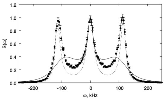
Figure 1. Fluctuation power spectra for the slow relaxation case ($p_0=0.01$). The spectra are normalized to the unit maximum value. Full line: 1T model; dotted line: frozen; dashed line: 2T model; symbols: DSMC.

Next, a situation where relaxation of internal energy is fast enough compared to the flow characteristic time (as determined by the speed of sound) is analyzed. In these conditions, we expect the one-temperature model to be accurate and that the two-temperature model will reduce to the former. The value $p_0=0.1$ has been chosen and gives for the relaxation time ${\tau }_0=7.0·{10}^{-6}s$ ($Z\equiv {\tau }_0/{\tau }_c=4.9$). Figure 2 shows the fluctuation power spectra as obtained from DSMC simulations and from the one-temperature and two-temperature models, respectively. For comparison, we also show the spectra predicted for the same gas when the bulk viscosity contribution is neglected (i.e., $\kappa =0$). In this case, it can be seen that both models describe the DSMC results accurately. Comparison with the $\kappa =0$ case also shows that this agreement is not trivial, since there is an important contribution of the bulk viscosity to the spectrum with $\frac{\kappa }{\eta }\approx 1$. Note, however, that the one-temperature model cannot describe the (small) change in the speed of sound that is a consequence of the finite relaxation time for internal energy.

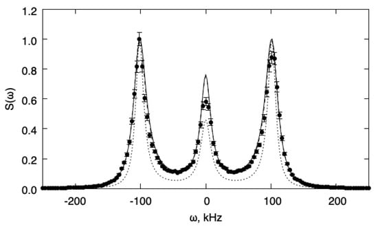
Figure 2. Fluctuation power spectra for the fast relaxation case ($p_0=0.1$). The spectra are normalized to unit maximum value. Full line: 1T model; dotted line: 1T model without bulk viscosity; dashed line: 2T model; symbols: DSMC.

The statistical error in the simulation results is around 4% for the slow relaxation and 12% for the fast relaxation case, respectively. Therefore, multi-temperature hydrodynamic equations, as derived from the Boltzmann transport equation, provide an adequate description of internal energy relaxation for all values of the relaxation time. Therefore, there is no need to invoke frequency-dependent transport coefficients that introduce unnecessary complications. Further, the results support the conclusion, obtained by kinetic theoretical arguments in the previous sections, that the multi-temperature model reduces to the one-temperature model when the relaxation time is small enough and that in this case, a bulk viscosity formalism is adequate.

These results are also relevant in view of the renewed interest in Rayleigh–Brillouin scattering in gases made possible by the use of nonlinear optical techniques [69]. Coherent Rayleigh–Brillouin scattering is a technique capable of making localized and high signal-to-noise ratio measurements of gases from the collisionless limit to the hydrodynamic regime. CRBS data are therefore expected to become a valuable source for the study of kinetic processes in molecular gases.

6. Numerical Experiments for a Quantum State Population

6.1. Internal Energy Spectrum and Energy-Exchange Collisions

The kinetic model that has been developed for arbitrary gas mixtures $\mathfrak{S}$ is specialized to $\mathfrak{S}=\{\mathrm{He},{\mathrm{H}}_2\}$ for the application. The required detailed cross sections used in this work has been calculated by the quasiclassical method, with an in-house developed code, which has been tested repeatedly against accurate results from the literature [43,44,45,46,47]. The set is complete, since all the ${\mathrm{H}}_2$ rovibrational states of the electronic ground state are considered initial and final states. Quasibound states and dissociation processes have also been considered in the trajectory calculations, even though they have not been used in the present study. Cross sections for the processes $\mathrm{He}+{\mathrm{H}}_2(v,\mathrm{J})\to \mathrm{He}+{\mathrm{H}}_2(w,k)$ with v/w initial/final vibrational states, j/k initial/final rotational states, have been calculated including both reactive (i.e., exchange) and nonreactive processes. Particular care has been taken in terms of the accuracy of trajectory calculation, with a strict checking at each step of each trajectory, in order to accurately determine the optimal time step and improve the overall computational efficiency [46]. The potential energy surface (PES) adopted in this study is the well known Muchnik–Russek [48], instead of the more recent BMP [49], used, for example, in a similar work by Kim et al. [50]. This choice is motivated by the important discrepancies found with respect to experimental data in Lee et al. [51]. Six billion trajectories, using $9.5$ years of CPU, have been calculated in this way on the Muchnik–Russek potential energy surface [48], using a constant density of 50,000 trajectories per eV of collisional energy (uniformly distributed) and per Å of impact parameter, in the range 1 meV–10 eV, with stratified sampling applied. Comparisons with available accurate quantum-mechanical theoretical data [52] put in evidence a very good reliability starting from 0.1–0.5 eV, depending on the initial states, corresponding to a minimal temperature of about 2000 K for rate coefficients [53]. For lower values of translational energies, cross sections tend to be less reliable, due to problems typical of nonreactive low-energy processes treated with QCT. A specific paper on this topic is in preparation. Finally, elastic collision integrals have been taken from Ref. [54].

The theoretical results of the previous sections are here specialized to the $\mathrm{He}$-${\mathrm{H}}_2$ mixture in thermal equilibrium conditions. The various contributions of the quantum state population as a function of temperature have been evaluated numerically. The procedure is analogous to that used in a previous study on the $\mathrm{H}$-${\mathrm{H}}_2$ mixture [27], to which the reader is referred for further details. Since a complete set of inelastic cross sections is available for the atom–diatom collisional system only, only a simulated gas is investigated, where ${\mathrm{H}}_2$-${\mathrm{H}}_2$ collisions are elastic. Since the resulting theoretical predictions are not amenable to experimental measurements, we resort to DSMC simulation and use Green–Kubo formulas for estimating the transport coefficients of the simulated gas.

A $\mathrm{He}$-${\mathrm{H}}_2$ mixture in thermal equilibrium conditions has been simulated with a standard DSMC code using a majorant frequency scheme [7]. For this application, a spatially homogeneous simulation is sufficient, so the code is run neglecting the particle movement, and no spatial mesh or boundary conditions need be specified. The VSS model has been used for the elastic collision cross sections, with parameters chosen to reproduce the transport coefficients in Ref. [54]. The number of simulated particles is 2000 for all cases discussed. Results have been averaged over a number of independent runs in order to reduce the statistical scatter r (typically ≈ 100). The latter is reported in the results as the simulation’s error bar.

6.2. Green–Kubo Bulk Viscosity in DSMC Simulations

Linear response theory is a powerful tool for the description of the relaxation towards thermodynamic equilibrium of any system subject to small perturbations. The fluctuation–dissipation theorem, in particular, connects the time correlation functions of mechanical quantities with the system transport properties. These relations are known as the Green–Kubo expressions for the transport coefficients [58]. This theory is independent of the mechanical model describing the system. It has been primarily applied to the evaluation of transport properties in Equilibrium Molecular Dynamics simulations of liquids [55] and solids (see, e.g., [56] and references therein). The Green–Kubo formulas have been applied to the evaluation of transport coefficients in DSMC simulations of dilute (i.e., ideal) gases.

For a system of volume V in equilibrium at temperature T and pressure p, the Green–Kubo formula for the bulk viscosity reads [57]:

$$\frac{4}{3}\eta +\kappa =\frac{1}{V}\frac{1}{k_{\mathrm{B}}T}{\int }_0^{+\infty }<({\mathrm{J}}_{xx}^p\left(0\right)-pV)({\mathrm{J}}_{xx}^p\left(\tau \right)-pV)>d\tau ,$$

(77)

where $<\cdots >$ denotes ensemble average, whereas that of the shear viscosity reads

$$\eta =\frac{1}{V}\frac{1}{k_{\mathrm{B}}T}{\int }_0^{+\infty }<{\mathrm{J}}_{xy}^p\left(0\right){\mathrm{J}}_{xy}^p\left(\tau \right)>d\tau .$$

(78)

The quantities ${\mathrm{J}}_{xx}^p$ or ${\mathrm{J}}_{xy}^p$, the currents, are, respectively, any of the diagonal or off-diagonal components of the spatially averaged, time dependent, rank-two pressure tensor:

$${\mathbf{J}}^p=\sum _i{m}_i{\mathit{C}}_i\otimes {\mathit{C}}_i-pV\mathit{I},$$

(79)

where the sum runs over simulated particles and $\mathit{C}={\mathit{c}}_i-\mathit{v}$.

The equilibrium condition allows us (via the ergodic hypothesis and stationarity) to express the integral in Equation (77) as the zero-frequency limit of the current power spectrum:

$$2{\int }_0^{+\infty }d\tau <(J_{xx}^p\left(0\right)-pV)(J_{xx}^p\left(\tau \right)-pV)>=\underset{T\to +\infty }{lim}\frac{1}{T}{\left|A_{xx}^p\left(0\right)\right|}^2,$$

(80)

$A_{xx}^p\left(\omega \right)$ being the current Fourier transform.

In DSMC simulation, the current $J^p$ is sampled at discrete time points, then Fourier transformed with standard FFT algorithms and squared. Let $P^{{\eta }_v}$ be the resulting zero-frequency value:

$$\frac{4}{3}\eta +\kappa =\frac{1}{V}\frac{1}{k_{\mathrm{B}}T}\frac{1}{2t_{sim}}{P}^{{\eta }_v}w{\Delta }_t^2.$$

(81)

$t_{sim}$ being the simulation duration, ${\Delta }_t$ the sampling time interval and w the weight of simulated particles (each particle representing w real particles). The factor w arises because the fluctuation amplitude is proportional to the square root of the number of simulated particles; the factor ${\Delta }_t^2$ comes from the discrete Fourier transform.

6.3. Results

The DSMC simulations have been performed for an equimolar mixture of helium and hydrogen with $n={10}^{20}{\mathrm{m}}^{-3}$. The resulting bulk viscosity obtained from DSMC is presented in Figure 3, together with the equilibrium viscosity as a function of temperature. The equilibrium bulk viscosity has been evaluated by using the expression

$$\kappa ={\left(\frac{c^{\mathrm{int}}}{c^{\mathrm{vl}}}\right)}^2\frac{{\left(k_{\mathrm{B}}T\right)}^3}{2\left[\left[{(\Delta E)}^2\right]\right]},$$

where $\left[\right[\left]\right]$ is the usual averaging operator and $\Delta E$ the energy jump during a collision of the simulated gas [9,26,27]. The DSMC calculations have been performed at temperatures $T=6000$ K, $T=9000$ K, and $T=$ 10,000 K.

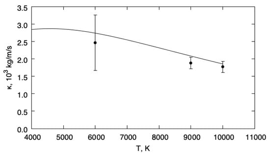
Figure 3. Bulk viscosities. Solid line: ${\kappa }^{\mathrm{e}}$; symbols: DSMC.

This figure reveals the very good agreement between the bulk viscosity of the fluctuating quantum population and the equilibrium limit, illustrating the accuracy of the least square formulation with a variational space ‘compatible with the equilibrium mixture’.

7. Fluid and Mathematical Aspects

7.1. Impact in Fluid Mechanics

The impact of the viscosity has scarcely been addressed in the past literature [70,71,72,73]. Karim [70] pointed out the importance of bulk viscosity coefficients and underlined that Stokes relation is only justified for monatomic gases. The impact of bulk viscosity on hypersonic boundary layers has been investigated in depth by Emmanuel [71,72]. A review of the concept of bulk viscosity and its implications for fluids over the twentieth century has been given by Graves and Argrow [73].

More recently, Billet et al. have investigated the interaction of a shock wave with a hydrogen bubble [74]. The bulk viscosity coefficient has been found to have a major influence on both the fluid and thermal aspects. This impact originates in particular from the thickening of pressure waves by bulk viscosity and from vorticity production when pressure and density gradients are not aligned. The artificial success of the Stokes approximation has also been related to the gradient structure of the term of $\mathbf{\nabla }·(\kappa \mathbf{\nabla }·\mathit{v}\mathit{I})=\mathbf{\nabla }(\kappa \mathbf{\nabla }·\mathit{v})$. This term is indeed absent in boundary layers at second order, and only has a Ma${}^2$ influence over fluid variables. As a typical example, in a steady hydrogen-air flame, $\kappa /\eta$ is not small; $\mathbf{\nabla }·\mathit{v}$ is not small either, but the gradient structure essentially leads to replacement of the hydrodynamic perturbed pressure $\tilde{p}$ by $\tilde{p}-\kappa \mathbf{\nabla }·\mathit{v}$, as discussed in Billet et al. [74]. Fru et al. have further investigated the small Mach situation and established that for a long-time integration the bulk viscosity regains its major influence [75]. The impact of bulk viscosity on compressible homogeneous turbulence has been studied by Chen et al., and the compressibility of the flow found significantly reduces when bulk viscosity is involved [98]. Two- and three-dimensional simulations of the interaction of a shock wave with a shear layer have further been investigated by Boukharfane et al. [76]. Finally, the interaction of a shock wave with a droplet has recently been studied by Singh et al., and bulk viscosity has again been found to play a major role [77].

Recent investigations have also shown that large values of bulk viscosity coefficients in dilute carbon dioxide mixtures result from erroneous applications of relaxation relations out of their domain of validity [11,13].

7.2. Chapman–Enskog Method for the Simplified Two-Temperature Model

The system of partial differential Equations (6)–(9) modeling two-temperature fluids derived in Section 2 may be written in the convenient vector form

$${\partial }_t^{}{\mathrm{u}}_{ϵ}+\sum _{i\in \mathcal{D}}{\mathrm{A}}_i\left(\mathrm{u}\right){\partial }_i^{}{\mathrm{u}}_{ϵ}-{ϵ}^{}\sum _{i,j\in \mathcal{D}}{\partial }_i^{}\left({\mathrm{B}}_{ij}\left({\mathrm{u}}_{ϵ}\right){\partial }_j^{}{\mathrm{u}}_{ϵ}\right)-\frac{1}{ϵ}\mathsf{\Omega }\left({\mathrm{u}}_{ϵ}\right)=0,$$

(82)

where ${\partial }_i^{}$ is the partial derivation in the ith spatial direction, $\mathcal{D}$ the indexing set of spatial directions, and ${\mathrm{u}}_{ϵ}$ the conservative variable given by

$${\mathrm{u}}_{ϵ}={\left(\rho ,\rho \mathit{v},{\mathcal{E}}_{\mathrm{tr}}+{\mathcal{E}}_{\mathrm{int}}+\frac{1}{2}\rho {\left|\mathit{v}\right|}^2,{\mathcal{E}}_{\mathrm{int}}\right)}^t.$$

(83)

In these Equation (82), the matrix ${\mathrm{A}}_i$ is the Jacobian ${\mathrm{A}}_i={\partial }_{\mathrm{u}}{\mathrm{F}}_i$ of the convective flux in the ith spatial direction ${\mathrm{F}}_i$, whereas the dissipative matrices ${\mathrm{B}}_{ij}$ are related to the dissipative fluxes $ϵ{\mathrm{F}}_i^{diss}$ with $ϵ{\mathrm{F}}_i^{diss}=-ϵ{\sum }_{j\in \mathcal{D}}{\mathrm{B}}_{ij}\left({\mathrm{u}}_{ϵ}\right){\partial }_j^{}{\mathrm{u}}_{ϵ}$. The convective flux ${\mathrm{F}}_i$ and dissipative flux $ϵ{\mathrm{F}}_i^{diss}$ in the ith spatial direction and source term $\mathsf{\Omega }$ are given by

$$\begin{array}{cc}\hfill {\mathrm{F}}_i& ={\left(\rho v_i,\rho \mathit{v}{v}_i+p{\mathrm{e}}_i,({\mathcal{E}}^{\mathrm{tr}}+{\mathcal{E}}^{\mathrm{int}}+\frac{1}{2}{\rho \left|\mathit{v}\right|}^2+p)v_i,{\mathcal{E}}^{\mathrm{int}}{v}_i\right)}^t,\hfill \end{array}$$

(84)

$$\begin{array}{cc}\hfill ϵ{\mathrm{F}}_i^{diss}& ={\left(0,{\mathit{\Pi }}_i,Q_i^{\mathrm{tr}}+Q_i^{\mathrm{int}}+{\mathit{\Pi }}_i·\mathit{v},Q_i^{\mathrm{int}}\right)}^t,\hfill \end{array}$$

(85)

$$\begin{array}{cc}\hfill \frac{1}{ϵ}\mathsf{\Omega }& ={\left(0,\mathbf{0},0,{\omega }^{\mathrm{int}}\right)}^t=\frac{1}{ϵ}{\left(0,\mathbf{0},0,\frac{\rho c^{\mathrm{int}}(T^{\mathrm{tr}}-T^{\mathrm{int}})}{{\overline{\tau }}^{\mathrm{int}}}\right)}^t,\hfill \end{array}$$

(86)

where ${\mathit{\Pi }}_i={({\Pi }_{1i},{\Pi }_{2i},{\Pi }_{3i})}^t$, ${\mathit{Q}}^{\mathrm{int}}={(Q_1^{\mathrm{int}},Q_2^{\mathrm{int}},Q_3^{\mathrm{int}})}^t$, and ${\mathit{Q}}^{\mathrm{tr}}={(Q_1^{\mathrm{tr}},Q_2^{\mathrm{tr}},Q_3^{\mathrm{tr}})}^t$. The convective matrices ${\mathrm{A}}_i$ and $i\in \mathcal{D}$, and the the dissipation matrices ${\mathrm{B}}_{ij}$, which contain all the transport coefficients, are investigated in [94,95,96]. Both the diffusion terms and the internal energy relaxation time have naturally been rescaled in the form $ϵ{\mathrm{B}}_{ij}$ and ${\tau }^{\mathrm{int}}=ϵ{\overline{\tau }}^{\mathrm{int}}$ where $ϵ$ is a typical Knudsen number. Two different small parameters could more generally be introduced with ${ϵ}_d$ in front of the dissipation terms and $ϵ$ for the relaxation of internal energy in (82), and an independent limit with ${ϵ}_d$ and $ϵ$ may also be investigated [94,95,96]. However, it is also legitimate and convenient to investigate the simpler situation where ${ϵ}_d=ϵ$ [94,95,96,97]. The dependence of the solution on the parameter $ϵ$ has been emphasized by denoting the conservative variable in the form ${\mathrm{u}}_{ϵ}$.

Symmetrized forms have been shown to be of fundamental importance for analyzing the mathematical structure of hyperbolic–parabolic systems of partial differential equations modeling fluids [22,78,79,80,81,82,83,84,85,86,87,88,89,90,91,92,93]. They are useful for a priori estimates, existence theorems [22,78,79,80,81,82,83,84,85,86,87,88,89,90,91,92,93] as well as finite element formulations [99]. The existence of a symmetrized form is related to the existence of a mathematical entropy compatible with convective terms, dissipative terms and relaxation of energy. Symmetrized forms for the system of partial differential equations modeling two-temperature fluid (82) have been comprehensively investigated under natural mathematical assumptions on thermodynamics and transport in [94,95,96]. Entropic as well as normal symmetrized forms have been obtained with an entropy compatible with convective, diffusive as well as source terms [94,95,96].

The concept of Chapman–Enskog expansion has also been extended to hyperbolic systems of partial differential equations by Liu [82] and Liu, Chen, Levermore [84] and later to hyperbolic–parabolic systems by Giovangigli and Yong [94,95,96,97]. The natural structural conditions are that there exists a mathematical entropy, taken for convenience as $\sigma =-S/R$, that is compatible with convection, diffusion as well as source terms [82,84,94,95,96,97]. It is also required that there exists an equilibrium manifold or slow manifold E, characterized by the relation $T^{\mathrm{tr}}=T^{\mathrm{int}}$ for the two-temperature problem, and the slow variable corresponding to (83) reads $u_{\mathrm{eq}}={\left(\rho ,\rho \mathit{v},\mathcal{E}+\frac{1}{2}\rho {\left|\mathit{v}\right|}^2\right)}^t$. For each slow variable $u_{\mathrm{eq}}$, there exists a unique ${\mathrm{u}}_{\mathrm{eq}}$, such that ${\mathsf{\Pi }}_{\mathrm{eq}}^t{\mathrm{u}}_{\mathrm{eq}}=u_{\mathrm{eq}}$ where ${\mathsf{\Pi }}_{\mathrm{eq}}$ is the projector operator on the slow manifold with matrix ${\mathsf{\Pi }}_{\mathrm{eq}}=[{\mathit{e}}_1,\dots ,{\mathit{e}}_4]$ with ${\mathit{e}}_i$, $1\le i\le 5$, denoting the canonical basis vectors of ${\mathbb{R}}^5$, and for later use, we also introduce the projector with matrix ${\mathit{\Pi }}_{\mathrm{rap}}=\left[{\mathit{e}}_5\right]$. The slow manifold is thus parameterized by $u_{\mathrm{eq}}$, and a careful analysis shows that the equilibrium one-temperature fluid model exactly corresponds to a second-order Chapman–Enskog [94,95,96] of the partial differential Equation (82). The schematic diagram of Figure 4 is thus obtained

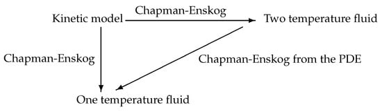
Figure 4. Schematic diagram of the double Chapman–Enskog procedure.

The Chapman–Enskog expansion for the solution ${\mathrm{u}}_{ϵ}$ to the system of partial differential Equation (82) is notably in the form

$${\mathrm{u}}_{ϵ}=\sum _{i\ge 0}{ϵ}^i{\overline{\mathrm{u}}}_i={\overline{\mathrm{u}}}_0+ϵ{\overline{\mathrm{u}}}_1+\mathcal{O}\left({ϵ}^2\right)$$

(87)

where the zeroth-order term ${\overline{\mathrm{u}}}_0$ coincides with ${\mathrm{u}}_{ϵ}$ on the slow manifold ${\mathsf{\Pi }}_{\mathrm{eq}}^t{\mathrm{u}}_{ϵ}={\mathsf{\Pi }}_{\mathrm{eq}}^t{\overline{\mathrm{u}}}_0=u_{\mathrm{eq}}$, where the Enskog constraints are in the form ${\mathsf{\Pi }}_{\mathrm{eq}}^t{\overline{\mathrm{u}}}_i=0$ for $i\ge 1$ and where ${\overline{\mathrm{u}}}_i$ only depends on ${\partial }^{\alpha }{\mathrm{u}}_{\mathrm{eq}}$ for $\left|\alpha \right|\le i$. Combining (82) with (87), the equations for ${\overline{\mathrm{u}}}_i$, $i\ge 0$, are given by

$$\begin{array}{c}{\partial }_t^{}({\overline{\mathrm{u}}}_0+ϵ{\overline{\mathrm{u}}}_1+\cdots )+\sum _{i\in \mathcal{D}}{\partial }_i^{}\left({\mathrm{F}}_i\left({\overline{\mathrm{u}}}_0\right)+ϵ{\partial }_{\mathrm{u}}^{}{\mathrm{F}}_i\left({\overline{\mathrm{u}}}_0\right){\overline{\mathrm{u}}}_1+\cdots \right)\\ -ϵ\sum _{i,j\in \mathcal{D}}{\partial }_i^{}\left({\mathrm{b}}_{ij}\left({\overline{\mathrm{u}}}_0\right){\partial }_j^{}{\overline{\mathrm{u}}}_0+\cdots \right)=\frac{1}{ϵ}\left(\mathsf{\Omega }\left({\overline{\mathrm{u}}}_0\right)+ϵ{\partial }_{\mathrm{u}}\mathsf{\Omega }\left({\overline{\mathrm{u}}}_0\right){\overline{\mathrm{u}}}_1+\cdots \right).\end{array}$$

At the order $-1$, it is found that $\mathsf{\Omega }\left({\overline{\mathrm{u}}}_0\right)=0$, so that ${\overline{\mathrm{u}}}_0$ is an equilibrium point ${\overline{\mathrm{u}}}_0={\mathrm{u}}_{\mathrm{eq}}\left(u_{\mathrm{eq}}\right)$ and the slow variable equations are given by

$${\partial }_t^{}{u}_{\mathrm{eq}}+\sum _{i\in \mathcal{D}}{\partial }_i^{}\left({\mathsf{\Pi }}_{\mathrm{eq}}^t{\mathrm{F}}_i\left({\overline{\mathrm{u}}}_0\right)+ϵ{\mathsf{\Pi }}_{\mathrm{eq}}^t{\partial }_{\mathrm{u}}^{}{\mathrm{F}}_i\left({\overline{\mathrm{u}}}_0\right){\overline{\mathrm{u}}}_1+\cdots \right)-ϵ\sum _{i,j\in \mathcal{D}}{\partial }_i^{}\left({\mathsf{\Pi }}_{\mathrm{eq}}^t{\mathrm{B}}_{ij}\left({\overline{\mathrm{u}}}_0\right){\partial }_j^{}{\overline{\mathrm{u}}}_0+\cdots \right)=0.$$

The equation at zeroth-order governing ${\overline{\mathrm{u}}}_0$ are found to be a symmetrizable hyperbolic system; indeed, Euler equations for the one-temperature fluid. The perturbed term ${\overline{\mathrm{u}}}_1$ is the next solution of linearized equations with the Enskog constraints in the form

$$\left\{\begin{array}{c}{\partial }_{\mathrm{u}}\mathsf{\Omega }\left({\overline{\mathrm{u}}}_0\right){\overline{\mathrm{u}}}_1={\partial }_t^{}{\overline{\mathrm{u}}}_0+\sum _{i\in \mathcal{D}}{\partial }_i^{}\left({\mathrm{F}}_i\left({\overline{\mathrm{u}}}_0\right)\right),\hfill \\ {\mathsf{\Pi }}_{\mathrm{eq}}^t{\overline{\mathrm{u}}}_1=0,\hfill \end{array}\right.$$

(88)

and using the Euler equation in order to express ${\partial }_t^{}{\overline{\mathrm{u}}}_0$, the first-order perturbation ${\overline{\mathrm{u}}}_1$ is found in the form

$${\overline{\mathrm{u}}}_1=-\sum _{j\in \mathcal{D}}{m}_j{\partial }_j^{}{u}_{\mathrm{eq}},$$

where ${\mathrm{M}}_j$ and $j\in \mathcal{D}$ are 5 × 4 matrices. The reader is referred to [94,95,96,97] for more details. The first-order Navier–Stokes-type equations are then obtained as

$${\partial }_t^{}{u}_{\mathrm{eq}}+\sum _{i\in \mathcal{D}}{\mathrm{A}}_i^{\mathrm{eq}}\left(u_{\mathrm{eq}}\right){\partial }_i^{}{u}_{\mathrm{eq}}-ϵ\sum _{i,j\in \mathcal{D}}{\partial }_i^{}\left({\mathrm{B}}_{ij}^{\mathrm{eq}}\left(u_{\mathrm{eq}}\right){\partial }_j^{}{u}_{\mathrm{eq}}\right)$$

(89)

with the diffusion coefficients in the form

$${\mathrm{B}}_{ij}^{\mathrm{eq}}\left(u_{\mathrm{eq}}\right)={\mathsf{\Pi }}_{\mathrm{eq}}^t{\mathrm{B}}_{ij}{\partial }_{u_{\mathrm{eq}}}{\mathrm{u}}_{\mathrm{eq}}+{\mathsf{\Pi }}_{\mathrm{eq}}^t{\mathrm{A}}_i^{\mathrm{eq}}{m}_j.$$

(90)

The resulting first-order accurate governing equations for the slow variable thus involves dissipative coefficients arising from perturbed convective terms ${\mathsf{\Pi }}_{\mathrm{eq}}^t{\mathrm{A}}_i^{\mathrm{eq}}{m}_j$, as well as inherited directly from the system out of equilibrium ${\mathsf{\Pi }}_{\mathrm{eq}}^t{\mathrm{B}}_{ij}$. Both the bulk viscosity term arising from the perturbed convective fluxes and the shear viscosity term inherited from the out-of-equilibrium viscous tensor are finally involved in the equilibrium viscous tensor. For the two-temperature model, it is indeed found that

$$ϵ\sum _{i\in \mathcal{D}}{\partial }_i^{}\left({\mathsf{\Pi }}_{\mathrm{eq}}^t{\partial }_{\mathrm{u}}^{}{\mathrm{F}}_i{\overline{\mathrm{u}}}_1\right)=-{\left(0,\mathbf{\nabla }·(\kappa \mathbf{\nabla }·\mathit{v}\mathit{I}),\mathbf{\nabla }·(\kappa \mathbf{\nabla }·\mathit{v}\mathit{v})\right)}^t,$$

(91)

so that the bulk viscosity coefficients are exactly obtained from the perturbed out-of-equilibrium convective terms in the Chapman–Enskog method, whereas the shear viscosity and thermal conductivity contributions are directly inherited from the out-of-equilibrium model [94,95,96,97].

7.3. Multiple Time Expansions for the Simplified Two-Temperature Model

Exact mathematical convergence results have further been obtained for the simplified two-temperature system of equations in the form (82) over the full space ${\mathbb{R}}^d$ for $1\le d\le 3$ [96,97]. The results and the method of proof differ depending on whether the initial data are well prepared with $T_{\mathrm{data}}^{\mathrm{tr}}=T_{\mathrm{data}}^{\mathrm{int}}$ or ill prepared with $T_{\mathrm{data}}^{\mathrm{tr}}\ne T_{\mathrm{data}}^{\mathrm{int}}$, where ${({\rho }_{\mathrm{data}},{\mathit{v}}_{\mathrm{data}},T_{\mathrm{data}}^{\mathrm{tr}},T_{\mathrm{data}}^{\mathrm{int}})}^t$ denotes the variable at initial time $t=0$. Both the well-prepared situation [96] and the ill-prepared situations [97] have been investigated, and only the ill-prepared situation results are summarized in this section.

The existence of solutions to the Cauchy problem with ill-prepared initial data has been established, as well as the validity of asymptotic composite expansions including initial-layer correctors. The results may be conveniently presented using the variable

$$w_{ϵ}={\left(\rho ,\rho \mathit{v},{\mathcal{E}}_{\mathrm{tr}}+{\mathcal{E}}_{\mathrm{int}}+\frac{1}{2}\rho {\left|\mathit{v}\right|}^2,\frac{1}{T^{\mathrm{tr}}}-\frac{1}{T^{\mathrm{int}}}\right)}^t={(u_{ϵ},q_{ϵ})}^t,$$

(92)

with the slow $u_{ϵ}$ and fast $q_{ϵ}$ components given by

$$\begin{array}{cc}\hfill u_{ϵ}& ={\mathsf{\Pi }}_{\mathrm{eq}}^t{w}_{ϵ}={\mathsf{\Pi }}_{\mathrm{eq}}^t{\mathrm{u}}_{ϵ}={\left(\rho ,\rho \mathit{v},{\mathcal{E}}_{\mathrm{tr}}+{\mathcal{E}}_{\mathrm{int}}+\frac{1}{2}\rho {\left|\mathit{v}\right|}^2\right)}^t\hfill \\ \hfill q_{ϵ}& ={\mathsf{\Pi }}_{\mathrm{rap}}^t{w}_{ϵ}\frac{1}{T^{\mathrm{tr}}}-\frac{1}{T^{\mathrm{int}}}.\hfill \end{array}$$

Multiple time expansions have been introduced in the form

$$w_{ϵ}=w_0(t,\mathit{x})+ϵw_1(t,\mathit{x})+w_0^{\mathrm{il}}(t/ϵ,\mathit{x})+ϵw_1^{\mathrm{il}}(t/ϵ,\mathit{x})+\mathcal{O}\left({ϵ}^2\right),$$

(93)

with an outer expansion involving the standard time t

$$w_0(t,x)+ϵw_1(t,x)+\mathcal{O}\left({ϵ}^2\right),$$

(94)

as well as initial layer correctors involving the fast time $\tau =t/ϵ$ in the form

$$w_0^{\mathrm{il}}(\tau ,x)+ϵw_1^{\mathrm{il}}(\tau ,x)+\mathcal{O}\left({ϵ}^2\right),$$

(95)

and such that $w_0^{\mathrm{il}}$ and $w_1^{\mathrm{il}}$ are exponentially decreasing with respect to the fast time $\tau =t/ϵ$. The equations governing each of the asymptotic expansion coefficients $u_0$, $u_1$, $q_0$, $q_1$ and $q_2$, where $w_0={(u_0,q_0)}^t$, $w_1={(u_1,q_1)}^t$, $w_2^{\prime }={(0,q_2)}^t$ may be obtained. The proper initial and boundary conditions may also be written by first expanding the initial conditions

$$w_{\mathrm{data}}=w_{\mathrm{data}0}+ϵw_{\mathrm{data}1}+\mathcal{O}\left({ϵ}^2\right),$$

where $w_{\mathrm{data}}={(u_{\mathrm{data}},q_{\mathrm{data}})}^t$ and then identifying $w_{2mu0}(·,0)+w_{2mu0}^{\mathrm{il}}(·,0)=w_{\mathrm{data}0}$ and $w_{2mu1}(·,0)+w_{2mu1}^{\mathrm{il}}(·,0)=w_{\mathrm{data}1}$, so that in particular, $u_0(·,0)=u_{\mathrm{data}0}$, $q_0(·,0)=0$, $u_0^{\mathrm{il}}(·,0)=0$, and $q_0^{\mathrm{il}}(·,0)=q_{\mathrm{data}0}$. The mathematical structure of the hyperbolic-type equations governing $u_0$ and $u_1$ then guarantee the existence of solutions over a finite time interval $[0,\overline{t}]$ under natural regularity assumptions [94,95,96,97]. Notably, an important role is played by the mathematical entropy $\sigma$ that allows symmetrization of the corresponding systems of partial differential equations, and that is taken in the form $\sigma =-\mathcal{S}/R$ for convenience. In addition, the initial layer correctors are shown to satisfy systems of differential equations with respect to the fast time. The existence of an exponentially decreasing global solution is then obtained by using the entropy as a Lyapunov function [97]. An important tool has also been the use of an improved truncated approximation in the form

$$w_{ϵ}^{\mathrm{a}}=w_0+ϵw_1+{ϵ}^2{w}_2^{\prime }+w_0^{\mathrm{il}}+ϵw_1^{\mathrm{il}},$$

(96)

including a fast component of the second-order term $w_2^{\prime }={(0,q_2)}^t$

It is then established that the out-of-equilibrium solution exists over a finite time interval $[0,\overline{t}]$, and the truncated approximation is second-order accurate with ${sup}_{t\in [0,\overline{t}]}{|w_{ϵ}\left(t\right)-w_{ϵ}^{\mathrm{a}}\left(t\right)|}_{L^{\infty }}\le C{ϵ}^2$ where C is a finite constant and ${\left|\mathsf{f}\right|}_{L^{\infty }}={sup}_{\mathit{x}\in {\mathbb{R}}^d}\left|\mathsf{f}\left(\mathit{x}\right)\right|$ denotes the $L^{\infty }$ norm of a function $\mathsf{f}$ over ${\mathbb{R}}^d$.

It may also be established that the Hilbert-type expansion $u_0+ϵu_1$ and the Chapman–Enskog solution at equilibrium $u_{\mathrm{eq}}$ are $\mathcal{O}\left({ϵ}^2\right)$ close, so that

$$\underset{t\in [0,\overline{t}]}{sup}{\left|u_{\mathrm{eq}}\left(t\right)-\left(u_0\left(t\right)+ϵu_1\left(t\right)\right)\right|}_{L^{\infty }}\le C{ϵ}^2.$$

Combining these results, it is then obtained that if $u_{ϵ}={\mathsf{\Pi }}_{\mathrm{eq}}^t{w}_{ϵ}={\mathsf{\Pi }}_{\mathrm{eq}}^t{\mathrm{u}}_{ϵ}$ then for $ϵ$ small enough

$$\underset{t\in [0,\overline{t}]}{sup}{\left|u_{ϵ}(·,t)-(u_{\mathrm{eq}}(·,t)+ϵu_1^{\mathrm{il}}(·,t/ϵ))\right|}_{L^{\infty }}\le C{ϵ}^2.$$

In other words, the out-of-equilibrium slow variable $u_{ϵ}$ is $\mathcal{O}\left({ϵ}^2\right)$ close to the Chapman–Enskog solution at equilibrium $u_{\mathrm{eq}}$, up to a first-order term $ϵu_1^{\mathrm{il}}(·,t/ϵ))$ that is exponentially decreasing with respect to the fast time $\tau =t/ϵ$ [97]. The zeroth-order initial layer corrector is also governed by the ordinary differential equation in the form ${\partial }_{\tau }(T^{\mathrm{tr}}-T^{\mathrm{int}})=-\frac{c_{\mathrm{vl}}}{c_{\mathrm{tr}}{\tau }^{\mathrm{int}}}(T^{\mathrm{tr}}-T^{\mathrm{int}})$ so that assuming for the sake of illustration that $c_{\mathrm{int}}$ and ${\tau }^{\mathrm{int}}$ constant yields that

$$T^{\mathrm{tr}}\left(\tau \right)=T+\left(T^{\mathrm{tr}}\left(0\right)-T\left(0\right)\right)exp\left(-\frac{c_{\mathrm{vl}}}{c_{\mathrm{tr}}}\frac{\tau }{{\tau }^{\mathrm{int}}}\right),$$

and $q_1=\frac{T^{\mathrm{int}}{\tau }^{\mathrm{int}}}{c_{\mathrm{tr}}{\left(T^{\mathrm{tr}}\right)}^2+c_{\mathrm{int}}{\left(T^{\mathrm{int}}\right)}^2}\mathbf{\nabla }·\mathit{v}$ that yields the bulk viscosity contributions of (91).

The mathematical theoretical results obtained concerning the Chapman–Enskog solution are thus in full agreement with the physical framework. Drawing a parallel with the traditional Chapman–Enskog, one may say that the slow or fluid variable is the one-temperature fluid variable $u_{\mathrm{eq}}$, the Mawellian distribution is the corresponding equilibrium two-temperature fluid variable ${\mathrm{u}}_{\mathrm{eq}}$, the linearized Boltzmann equations are replaced by (88) and the resulting dissipative coefficients have two different sources with (90).

8. Conclusions

The relaxation of internal energy and the concept of bulk viscosity have been investigated in nonequilibrium gas models derived from the kinetic theory. Two-temperature models of single fluids and state-to-state models for mixtures of gases have been considered. When the rates for internal energy exchanges are smaller than the fluid time, a common interpretation of the apparition of the bulk viscosity coefficient has been obtained with (20), (46), and (67). The Monte Carlo simulations of spontaneous fluctuations near thermal equilibrium obtained by solving the Boltzmann equation have been shown to be in full agreement with the fluid models, provided the internal energy relaxation times are smaller than the fluid time. Numerical simulation of He-H${}_2$ quantum populations also yields bulk viscosity coefficients in agreement with the equilibrium. Mathematical aspects of internal energy relaxation have also been discussed for the two-temperature fluid model and were found to agree with the formal expansions. In particular, Chapman–Enskog expansions from systems of partial differential equations have been discussed, as well as rigorous results in the situation of ill-prepared initial data in full agreement with the formal expansions. A practical consequence of these results is that bulk viscosity should be systematically included in the numerical simulation of compressible fluids. Future work should also consider bulk viscosity coefficients arising in coarse-grained models, as well as numerical simulations with multiple internal energy modes and, more generally, states far from thermodynamic equilibrium.

References

- Capitelli, M.; Armenise, I.; Bruno, D.; Cacciatore, M.; Celiberto, R.; Colonna, G.; de Pascale, O.; Diomede, P.; Esposito, F.; Gorse, C.; et al. Non-equilibrium Plasma Kinetics: A state-to-state approach. Plasma Sourc. Sci. Tech. 2007, 16, S30–S44. [Google Scholar] [CrossRef]
- Colonna, G.; Armenise, I.; Bruno, D.; Capitelli, M. Reduction of state-to-state kinetics to macroscopic models in hypersonic flows. J. Thermophys. Heat Transf. 2006, 20, 477–486. [Google Scholar] [CrossRef]
- Chikhaoui, A.; Dudon, J.P.; Kustova, E.V.; Nagnibeda, E.A. Transport properties in reacting mixture of polyatomic gases. Physica A 1997, 247, 526–552. [Google Scholar] [CrossRef]
- Kustova, E.V.; Nagnibeda, E.A. Transport properties of a reacting gas mixture with strong vibrational and chemical nonequilibrium. Chem. Phys. 1998, 233, 57–75. [Google Scholar] [CrossRef]
- Kustova, E.V. On the simplified state-to-state transport coefficients. Chem. Phys. 2001, 270, 177–195. [Google Scholar] [CrossRef]
- Kustova, E.V.; Nagnibada, E.A.; Chikhaoui, A. On the accuracy of nonequilibrium transport coefficients calculation. Chem. Phys. 2001, 270, 459–469. [Google Scholar] [CrossRef]
- Bruno, D.; Capitelli, M.; Esposito, F.; Longo, S.; Minelli, P. Direct simulation of non-equilibrium kinetics under shock conditions in nitrogen. Chem. Phys. Lett. 2002, 360, 31–37. [Google Scholar] [CrossRef]
- Zhdanov, V.M. Transport Processes in Multicomponent Plasmas; Taylor and Francis: London, UK, 2002. [Google Scholar]
- Nagnibeda, E.; Kustova, E. Non-Equilibrium Reacting Gas Flow; Springer: Berlin/Heidelberg, Germany, 2009. [Google Scholar]
- Brun, R. Introduction to Reactive Gas Dynamics; Oxford University Press: Oxford, UK, 2009. [Google Scholar]
- Kustova, E. On the role of bulk viscosity and relaxation pressure in non-equilibrium flows. Aip Conf. Proc. 2009, 1084, 807–812. [Google Scholar]
- Kustova, E.V.; Nagnibeda, E.A. Kinetic model for multi-temperature flows of reacting carbon dioxide mixture. Chem. Phys. 2012, 398, 111–117. [Google Scholar] [CrossRef]
- Kustova, E.; Mekhonoshina, M. Models for bulk viscosity in carbon dioxide. Aip Conf. Proc. 2019, 2132, 150006. [Google Scholar]
- Munafò, A.; Panesi, M.; Magin, T.E. Boltzmann rovibrational collisional coarse-grained model for internal energy excitation and dissociation in hypersonic flows. Phys. Rev. E 2014, 89, 023001. [Google Scholar] [CrossRef]
- Munafò, A.; Liu, Y.; Panesi, M. Modeling of dissociation and energy transfer in shock-heated nitrogen flows. Phys. Fluids 2015, 27, 127101. [Google Scholar] [CrossRef]
- Kohler, M. Reibung in mäsig verdünnten gasen als folge verzögerter einstellung der energie. Zeitschr. Phys. 1949, 125, 715–732. [Google Scholar] [CrossRef]
- Hirschfelder, J.O.; Curtiss, C.F.; Bird, R.B. Molecular Theory of Gases and Liquids; Wiley: New York, NY, USA, 1954. [Google Scholar]
- Waldmann, L.; Trübenbacher, E. Formale kinetische Theorie von Gasgemischen aus anregbaren molekülen. Zeitschr. Naturforschg. 1962, 17, 363–376. [Google Scholar] [CrossRef]
- Chapman, S.; Cowling, T.G. The Mathematical Theory of Non-Uniform Gases; Cambridge University Press: Cambridge, UK, 1970. [Google Scholar]
- Ferziger, J.H.; Kaper, H.G. Mathematical Theory of Transport Processes in Gases; North Holland Publishing Company: Amsterdam, The Netherlands, 1972. [Google Scholar]
- McCourt, F.R.; Beenakker, J.J.; Köhler, W.E.; Kuscer, I. Non Equilibrium Phenomena in Polyatomic Gases; Volume I: Dilute Gases, Volume II: Cross Sections, Scattering and Rarefied Gases; Clarendon Press: Oxford, UK, 1990. [Google Scholar]
- Giovangigli, V. Multicomponent Flow Modeling; Birkhaüser: Boston, MA, USA, 1999. [Google Scholar]
- Ern, A.; Giovangigli, V. The Kinetic equilibrium regime. Physica-A 1998, 260, 49–72. [Google Scholar] [CrossRef]
- de Groot, S.R.; Mazur, P. Non-Equilibrium Thermodynamics; Dover Publications, Inc.: New York, NY, USA, 1984. [Google Scholar]
- Keizer, J. Statistical Thermodynamics of Nonequilibrium Processes; Springer: New York, NY, USA, 1987. [Google Scholar]
- Bruno, D.; Giovangigli, V. Relaxation of internal temperature and volume viscosity. Phys. Fluids 2011, 23, 093104, Erratum in Phys. Fluids 2013, 25, 039902. [Google Scholar] [CrossRef]
- Bruno, D.; Esposito, F.; Giovangigli, V. Relaxation of rotational-vibrational energy and volume viscosity in H-H2 Mixtures. J. Chem. Phys. 2013, 138, 084302. [Google Scholar] [CrossRef]
- Bruno, D.; Esposito, E.; Giovangigli, V. Relaxation of quantum state population and volume viscosities in He/H2 mixtures. Aip Conf. Proc. 2014, 1628, 1237–1244. [Google Scholar]
- Hermans, P.W.; Hermans, L.F.J.; Beenakker, J.J.M. A survey of experimental data related to the non-spherical interaction for the hydrogen isotopes and their mixture with noble gases. Physica A 1983, 122, 173–211. [Google Scholar] [CrossRef]
- Prangsma, G.J.; Borsboom, L.J.M.; Knaap, H.F.P.; den Meijdenberg, C.J.N.V.; Beenakker, J.J.M. Rotational relaxation in ortho Hydrogen between 170 and 300 K. Physica 1972, 61, 527–538. [Google Scholar] [CrossRef]
- Prangsma, G.J.; Alberga, A.H.; Beenakker, J.J.M. Ultrasonic determination of the volume viscosity of N2, CO, CH4, and CD4 between 77 and 300K. Physica 1973, 64, 278–288. [Google Scholar] [CrossRef]
- Tisza, L. Supersonic absorption and Stokes viscosity relation. Phys. Rev. 1941, 61, 531–536. [Google Scholar] [CrossRef]
- Turfa, A.F.; Knaap, H.F.P.; Thijsse, B.J.; Beenakker, J.J.M. A classical dynamics study of rotational relaxation in nitrogen gases. Physical A 1982, 112, 19–28. [Google Scholar] [CrossRef]
- Ern, A.; Giovangigli, V. Multicomponent Transport Algorithms; Lecture Notes in Physics, New series Monographs; Springer: Berlin/Heidelberg, Germany, 1994; Volume 24. [Google Scholar]
- Ern, A.; Giovangigli, V. Volume viscosity of dilute polyatomic gas mixtures. Eur. J. Mech. B/Fluids 1995, 14, 653–669. [Google Scholar]
- Mansour, M.M.; Garcia, A.L.; Lie, G.C.; Clementi, E. Fluctuating Hydrodynamics in a Dilute Gas. Phys. Rev. Lett. 1987, 58, 874–877. [Google Scholar] [CrossRef]
- Bruno, D.; Capitelli, M.; Longo, S.; Minelli, P. Monte Carlo simulation of light scattering spectra in atomic gases. Chem. Phys. Lett. 2006, 422, 571–574. [Google Scholar] [CrossRef]
- Ivanov, M.S.; Gimelshein, S.F. Computational hypersonic rarefied flows. Annu. Rev. Fluid Mech. 1998, 30, 469–505. [Google Scholar] [CrossRef]
- Oran, E.; Oh, C.; Cybyk, B. Direct simulation Monte Carlo: Recent advances and applications. Ann. Rev. Fluid Mech. 1998, 30, 403–441. [Google Scholar] [CrossRef]
- Bird, G. Recent advances and current challenges for DSMC. Comp. Math. App. 1998, 35, 1–14. [Google Scholar] [CrossRef]
- Frezzotti, A. A particle scheme for the numerical solution of the Enskog equation. Phys. Fluids 1997, 9, 1329–1335. [Google Scholar] [CrossRef]
- Bruno, D.; Capitelli, M.; Longo, S.; Minelli, P.; Taccogna, F. Particle kinetic modelling of rarefied gases and plasmas. Plasma Sources Sci. Technol. 2003, 12, 89–97. [Google Scholar] [CrossRef]
- Esposito, F.; Gorse, C.; Capitelli, M. Quasi-classical dynamics calculations and state-selected rate coefficients for H + H2(v,j)↦ 3H processes: Application to the global dissociation rate under thermal conditions. Chem. Phys. Lett. 1999, 303, 636–640. [Google Scholar] [CrossRef]
- Esposito, F.; Capitelli, M. Dynamical calculations of state to state and dissociation cross-sections for atom-molecule collision processes in hydrogen. At. Plasma-Mater. Interact. Data Fusion 2001, 9, 65–73. [Google Scholar]
- Esposito, F.; Capitelli, M. Quasiclassical trajectory calculations of vibrationally specific dissociation cross-sections and rate constants for the reaction O+O2(v)↦ 3O. Chem. Phys. Lett. 2002, 364, 180–187. [Google Scholar] [CrossRef]
- Esposito, F.; Capitelli, M. QCT calculations for the process N2(v) + N ↦ N2(v′) + N in the whole vibrational range. Chem. Phys. Lett. 2006, 418, 581–585. [Google Scholar] [CrossRef]
- Esposito, F.; Capitelli, M. Selective Vibrational Pumping of Molecular Hydrogen via Gas Phase Atomic Recombination. J. Phys. Chem. A 2009, 113, 15307–15314. [Google Scholar] [CrossRef]
- Muchnick, P.; Russek, A. The HeH2 energy surface. J. Chem. Phys. 1994, 100, 4336–4346. [Google Scholar] [CrossRef]
- Boothroyd, A.I.; Martin, P.G.; Peterson, M.R. Accurate analytic He-H2 potential energy surface from a greatly expanded set of ab initio energies. J. Chem. Phys. 2003, 119, 3187–3192. [Google Scholar] [CrossRef]
- Kim, J.G.; Kwon, O.J.; Park, C. Master Equation Study and Nonequilibrium Chemical Reactions for H + H2 and He + H2. J. Therm. Heat Transfer 2009, 23, 443–453. [Google Scholar] [CrossRef]
- Lee, T.-G.; Rochow, C.; Martin, R.; Clark, T.K.; Forrey, R.C.; Balakrishnan, N.; Stancil, P.C.; Schultz, D.R.; Dalgarno, A.; Ferland, G.J. Close-coupling calculations of low-energy inelastic and elastic processes in 4He collisions with H2: A comparative study of two potential energy surfaces. J. Chem. Phys. 2005, 122, 024307. [Google Scholar] [CrossRef]
- Balakrishnan, N.; Vieira, M.; Babb, J.; Dalgarno, A.; Forrey, R.; Lepp, S. Rate Coefficients for Ro-vibrational Transitions in H2 Due to Collisions with He. Astrophys. J. 1999, 524, 1122–1130. [Google Scholar] [CrossRef]
- Orlikowski, T. Close-coupling calculations of the cross sections and relaxation rates for ro-vibrational transitions in H2 colliding with He. Chem. Phys. 1981, 61, 405–413. [Google Scholar] [CrossRef]
- Bruno, D.; Catalfamo, C.; Capitelli, M.; Colonna, G.; Pascale, O.D.; Diomede, P.; Gorse, C.; Laricchiuta, A.; Longo, S.; Giordano, D.; et al. Transport properties of high-temperature Jupiter atmosphere components. Phys. Plasmas 2010, 17, 112315. [Google Scholar] [CrossRef]
- Evans, D.J.; Morriss, G. Statistical Mechanics of Nonequilibrium Liquids; Cambridge University Press: Cambridge, UK, 2008. [Google Scholar]
- McGaughey, A.J.H.; Kaviany, M. Quantitative validation of the Boltzmann transport equation phonon thermal conductivity model under the single-mode relaxation time approximation. Phys. Rev. B 2004, 69, 094303. [Google Scholar] [CrossRef]
- Boon, J.P.; Yip, S. Hydrodynamic Fluctuations. In Molecular Hydrodynamics; Dover: New York, NY, USA, 1991; pp. 237–278. [Google Scholar]
- Kubo, R.; Toda, M.; Hashitsume, N. Fluctuation and Dissipation Theorem. In Statistical Physics II; Springer: Berlin/Heidelberg, Germany, 1978; pp. 167–170. [Google Scholar]
- Berne, B.J.; Pecora, R. Light Scattering From Hydrodynamic Modes. In Dynamic Light Scattering; Dover: New York, NY, USA, 2000; pp. 223–246. [Google Scholar]
- Einstein, A. Theorie der Opaleszenz von homogenen Flüssigkeiten und Flüssigkeitsgemischen in der Nähe des kritischen Zustandes. Ann. Physik 1910, 33, 1275–1298. [Google Scholar] [CrossRef]
- Mountain, R.D. Spectral Distribution of Scattered Light in a Simple Fluid. Rev. Mod. Phys. 1966, 38, 205–214. [Google Scholar] [CrossRef]
- Jaeger, F.; Matar, O.K.; Müller, E.A. Bulk viscosity of molecular fluids. J. Chem. Phys. 2018, 148, 174504. [Google Scholar] [CrossRef]
- Sharma, B.; Kumar, R. Estimation of bulk viscosity of dilute gases using a nonequilibrium molecular dynamics approach. Phys. Rev. E 2019, 100, 013309. [Google Scholar] [CrossRef]
- Sharma, B.; Kumar, R.; Gupta, P.; Pareek, S.; Singh, A. On the estimation of bulk viscosity of dilute nitrogen gas using equilibrium molecular dynamics approach. Phys. Fluids 2022, 34, 057104. [Google Scholar] [CrossRef]
- Lifshitz, E.M.; Pitaevskii, L.P. Fluctuations of the Distribution Function in an Equilibrium Gas. In Physical Kinetics; Butterworth-Heinemann: Oxford, UK, 1995; pp. 79–84. [Google Scholar]
- Koura, K.; Matsumoto, H. Variable Soft Sphere Molecular Model for Inverse-Power-Law or Lennard-Jones Potential. Phys. Fluids A 1991, 3, 2459–2465. [Google Scholar] [CrossRef]
- Landau, L.D.; Lifshitz, E.M. Spatial Correlation of Density Fluctuations. In Statistical Physics; Part 1; Butterworth-Heinemann: Oxford, UK, 1980; pp. 350–353. [Google Scholar]
- Tysanner, M.W.; Garcia, A.L. Non-equilibrium behaviour of equilibrium reservoirs in molecular simulations. Int. J. Numer. Meth. Fluids 2005, 48, 1337–1349. [Google Scholar] [CrossRef]
- Pan, X.; Shneider, M.N.; Miles, R.B. Coherent Rayleigh-Brillouin scattering in molecular gases. Phys. Rev. A 2004, 69, 033814. [Google Scholar] [CrossRef]
- Karim, S.M.; Rosenhead, L. The second coefficient of viscosity of Liquids and gases. Rev. Mod. Phys. 1952, 24, 108–116. [Google Scholar] [CrossRef]
- Emanuel, G. Bulk viscosity of a dilute polyatomic gas. Phys. Fluids A 1990, 2, 2252–2254. [Google Scholar] [CrossRef]
- Emanuel, G. Effect of bulk viscosity on a hypersonic boundary layer. Phys. Fluids A 1992, 4, 491–495. [Google Scholar] [CrossRef]
- Graves, R.E.; Argrow, B. Bulk viscosity: Past to present. J. Thermophys. Heat Transf. 1999, 13, 337–342. [Google Scholar] [CrossRef]
- Billet, G.; Giovangigli, V.; de Gassowski, G. Impact of volume viscosity on a shock/hydrogen bubble interaction. Comb. Theory Model. 2008, 12, 221–248. [Google Scholar] [CrossRef]
- Fru, G.; Janiga, G.; Thevenin, D. Impact of Volume Viscosity on the Structure of Turbulent Premixed Flames in the Thin Reaction Zone Regime. Flow Turb. Combust. 2012, 88, 451–478. [Google Scholar] [CrossRef]
- Boukharfane, R.; Ferrer, P.J.M.; Mura, A.; Giovangigli, V. On the role of bulk viscosity in compressible reactive shear layer developments. Eur. J. Mech. B/Fluids 2019, 77, 32–47. [Google Scholar] [CrossRef]
- Singh, S.; Battiato, M.; Myong, R.S. Impact of bulk viscosity on flow morphology of shock-accelerated cylindrical light bubble in diatomic and polyatomic gases. Phys. Fluids 2021, 33, 066103. [Google Scholar] [CrossRef]
- Godunov, S. An interesting class of quasilinear systems. Sov. Math. Dokl. 1961, 2, 947–949. [Google Scholar]
- Friedrichs, K.O.; Lax, P.D. Systems of conservation laws with a convex extension. Proc. Nat. Acad. Sci. USA 1971, 68, 1686–1688. [Google Scholar] [CrossRef] [PubMed]
- Vol’pert, A.I.; Hudjaev, S.I. On the Cauchy problem for composite systems of nonlinear differential equations. Math USSR Sb. 1972, 16, 517–544. [Google Scholar] [CrossRef]
- Kawashima, S. Systems of a Hyperbolic-Parabolic Composite Type, with Applications to the Equations of Magnetohydrodynamics. Doctoral Thesis, Kyoto University, Kyoto, Japan, 1984. [Google Scholar]
- Liu, T.P. Hyperbolic Conservation Laws with Relaxation. Comm. Math. Phys. 1987, 108, 153–175. [Google Scholar] [CrossRef]
- Kawashima, S.; Shizuta, Y. On the normal form of the symmetric hyperbolic-parabolic systems associated with the conservation laws. Tôhoku Math. J. 1988, 40, 449–464. [Google Scholar] [CrossRef]
- Chen, G.Q.; Levermore, C.D.; Liu, T.-P. Hyperbolic conservation laws with stiff relaxation terms and entropy. Comm. Pure Appl. Math. 1994, 47, 787–830. [Google Scholar] [CrossRef]
- Serre, D. Systèmes de Lois de Conservation I et II; Diderot Editeur, Art et Science: Paris, France, 1996. [Google Scholar]
- Giovangigli, V.; Massot, M. Asymptotic stability of equilibrium states for multicomponent reactive flows. Math. Mod. Meth. App. Sci. 1998, 8, 251–297. [Google Scholar] [CrossRef]
- Dafermos, C. Hyperbolic Conservation Laws in Continuum Physics; Springer: Berlin/Heidelberg, Germany, 2000. [Google Scholar]
- Yong, W.-A.; Zumbrun, K. Existence of relaxation shock profiles for hyperbolic conservation laws. Siam J. Appl. Math. 2000, 60, 1665–1675. [Google Scholar]
- Feireisl, E. Dynamics of Viscous Compressible Fluids; Oxford University Press: Oxford, UK, 2004. [Google Scholar]
- Yong, W.-A. Entropy and global existence for hyperbolic balance laws. Arch. Rat. Mech. Anal. 2004, 172, 247–266. [Google Scholar] [CrossRef]
- Kawashima, S.; Yong, W.-A. Dissipative structure and entropy for hyperbolic systems of conservation laws. Arch. Rat. Mech. Anal. 2004, 174, 345–364. [Google Scholar] [CrossRef]
- Bresch, D.; Desjardins, B. On the existence of global weak solutions to the Navier-Stokes equations for viscous compressible and heat conducting fluids. J. Math. Pure Appl. 2007, 87, 57–90. [Google Scholar] [CrossRef]
- Serre, D. The Structure of Dissipative Viscous System of Conservation laws. Phys. D 2010, 239, 1381–1386. [Google Scholar] [CrossRef]
- Giovangigli, V.; Yong, W.-A. Volume Viscosity and Internal Energy Relaxation: Symmetrization and Chapman-Enskog Expansion. Kin. Rel. Model. 2015, 8, 79–116. [Google Scholar] [CrossRef]
- Giovangigli, V.; Yong, W.-A. Erratum: Volume Viscosity and Internal Energy Relaxation: Symmetrization and Chapman-Enskog Expansion. Kin. Rel. Model. 2016, 9, 813. [Google Scholar] [CrossRef][Green Version]
- Giovangigli, V.; Yong, W.-A. Volume Viscosity and Internal Energy Relaxation: Error Estimates. Nonlinear Anal. Real World Appl. 2018, 43, 213–244. [Google Scholar] [CrossRef]
- Giovangigli, V.; Yang, Z.B.; Yong, W.-A. Relaxation Limit and Initial-Layer for a Class of Hyperbolic-Parabolic Systems. SIAM J. Math. Anal. 2018, 50, 4655–4697. [Google Scholar] [CrossRef]
- Chen, S.; Wang, X.; Wang, J.; Wan, M.; Li, H.; Chen, S. Effect of bulk viscosity on compressible homogeneous turbulence. Phys. Fluids 2019, 31, 085115. [Google Scholar]
- Hughes, T.J.R.; Franca, L.P.; Mallet, M. A new finite element formulation for computational fluid dynamics: I. Symmetric forms of the compressible Euler and Navier-Stokes equations and the second law of thermodynamics. Comp. Meth. Appl. Mech. Eng. 1986, 54, 223–234. [Google Scholar] [CrossRef]
Publisher’s Note: MDPI stays neutral with regard to jurisdictional claims in published maps and institutional affiliations. |
© 2022 by the authors. Licensee MDPI, Basel, Switzerland. This article is an open access article distributed under the terms and conditions of the Creative Commons Attribution (CC BY) license (https://creativecommons.org/licenses/by/4.0/).