Article

Hybrid Neural Network Reduced Order Modelling for Turbulent Flows with Geometric Parameters

1
MathLab, Mathematics Area, SISSA, International School for Advanced Studies, Via Bonomea 265, I-34136 Trieste, Italy
2
Volkswagen AG, Innovation Center Europe, 38436 Wolfsburg, Germany
*
Author to whom correspondence should be addressed.
Fluids 2021, 6(8), 296; https://doi.org/10.3390/fluids6080296
Submission received: 30 June 2021 / Revised: 5 August 2021 / Accepted: 11 August 2021 / Published: 22 August 2021
(This article belongs to the Special Issue Reduced Order Models for Computational Fluid Dynamics)

Abstract

:
Geometrically parametrized partial differential equations are currently widely used in many different fields, such as shape optimization processes or patient-specific surgery studies. The focus of this work is some advances on this topic, capable of increasing the accuracy with respect to previous approaches while relying on a high cost–benefit ratio performance. The main scope of this paper is the introduction of a new technique combining a classical Galerkin-projection approach together with a data-driven method to obtain a versatile and accurate algorithm for the resolution of geometrically parametrized incompressible turbulent Navier–Stokes problems. The effectiveness of this procedure is demonstrated on two different test cases: a classical academic back step problem and a shape deformation Ahmed body application. The results provide insight into details about the properties of the architecture we developed while exposing possible future perspectives for this work.

1. Introduction

Shape optimization in the context of turbulent flow problems is a particularly challenging task. The difficulty is linked with both the high dimensionality of the problems that need to be solved and the number of configurations to test, the former due to the physics and the latter due to the scope of the research. These two features usually make the problem intractable with standard numerical methods (e.g., finite element, finite volume, finite difference methods). Reduced order models [1,2] (ROMs) are a possible tool that can be used in such a setting to make the problem solvable. There exists a variety of reduced order modelling techniques, but the overall principle of all of them is to unveil a low dimensional behaviour of a high dimensional system to allow faster computation.
ROMs can be classified depending on the technique used to approximate the solution manifold and the method used to evolve the latent dynamics. The most used techniques to evaluate the solution manifold are based on linear approximation methods such as the reduced basis with a greedy approach [3,4], the proper orthogonal decomposition [5], or nonintrusive methods as exposed in [6], but more recently nonlinear methods have also been proposed [7,8]. Concerning the evolution of the latent space dynamics, arguably the most common approach is based on the (Petrov–) Galerkin projection of the original system onto the reduced subspace/manifold [9]. Data driven techniques [10], which are solely based on the reconstruction of the mapping between input and output quantities, are also a possible approach. Recently, these techniques also received particular attention due to the latest discoveries in machine learning. Data-driven methods are usually easier to implement and also permit obtaining efficient ROMs in the case of nonlinear/nonaffine problems and in the case of commercial codes with no access to the discretized full order system. On the other hand, they usually do not exploit information concerning the underlying physical principles, and they might require a large number of training data to produce accurate results. Projection-based techniques, thanks to the projection stage, incorporate physical knowledge in a natural way but are particularly challenging to be implemented in the case of nonlinear and nonaffine problems.
In this work, we propose a hybrid approach where the underlying partial differential equations are partially treated using a standard POD–Galerkin approach and partially by neural networks data-driven approaches. This choice is dictated by both practical and theoretical considerations. The practical consideration concerns the idea of generating an approach that could be applied to any turbulence model without the need to modify the reduced order model.
Turbulence is a complex phenomena which does not yet have a universal theory. For practical problems, the numerical resolution of the Navier–Stokes equations up to the Kolmogorov scale where kinetic energy is converted into internal energy by viscous stresses would require an intractable number of degrees of freedom and an extremely refined time step. Even with modern supercomputers, direct numerical simulation is still unfeasible. There exist different approaches to make the simulation of turbulent flows numerically feasible, such as Reynolds-averaged Navier–Stokes equations (RANS) or large eddy simulation approaches with turbulence modelling. In this work, we have decided to rely on a RANS approach at the full order level which offers a good compromise between accuracy and computational cost. It is out of the scope of this article to offer a comprehensive introduction on turbulence models or to propose advances on mathematical aspects of turbulence. Therefore, we refer the reader to classical textbooks on turbulence modelling and mathematical aspects of turbulence [11,12,13].
In incompressible turbulent flows, there exist a large number of turbulence models, used to outflank the difficulty in solving the dissipative scales, and using a projection-based technique would require creating a new reduced order model for each of them. Secondly, despite the large amount of theoretical work behind turbulence models, there are still a number of empirical coefficients, and this makes the overall formulation less rigorous in terms of physical principles. These considerations have been used to propose a reduced order model that could be applied to any eddy viscosity turbulence model and that exploits a projection-based technique for mass and momentum conservation and a data-driven approach for the reconstruction of the eddy viscosity field. The model is constructed extending the work done in [14,15] to geometrically parametrized problems [16] with a modification of the approach to reconstruct the eddy viscosity mapping.
In the first part of this work, we present all the technicalities related to the implementation of the previously described hybrid method: Section 2.1 contains the finite volume discretization of the incompressible Navier–Stokes equation employed for this work, Section 2.2 explains the method we selected for the motion of the mesh due to geometrical parametrization, Section 2.3 introduces the reduced order model, Section 2.4 gives an overview of the actual algorithm used for the resolution, and Section 2.5 treats the eddy viscosity evaluation. The second part of the paper is devoted to the presentation of the results related to two different test cases: a classical academic back step with variable slope of the step into Section 3.1 and a second, more applied one, shown in Section 3.2, where the flow around an Ahmed body with variable slope of the rear part is resolved, both revealing good behaviours and promising results. In the end, a few considerations and possible future developments for this work are presented in Section 4.

2. Models and Methods

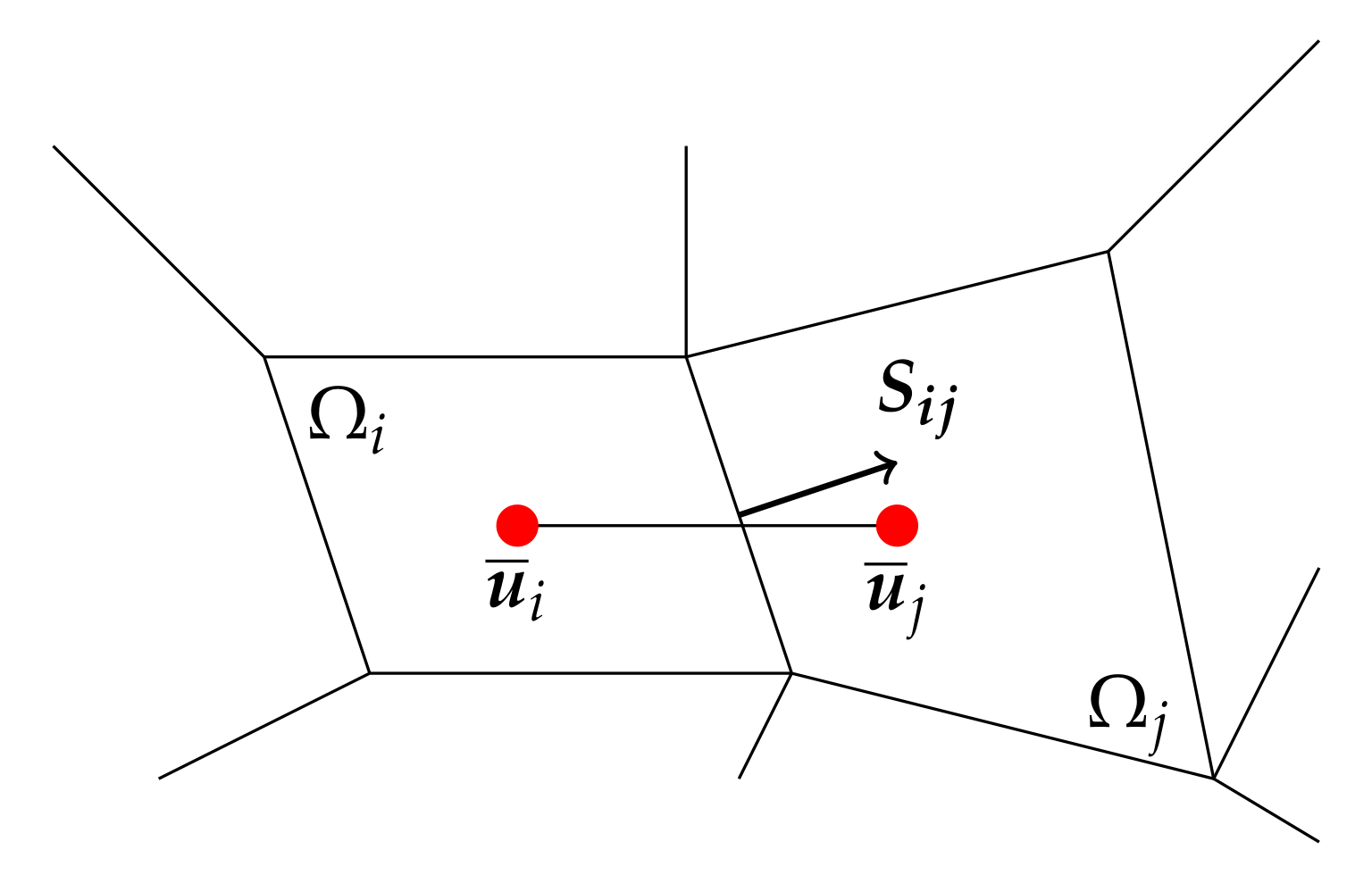
2.1. The Full Order Problem

In this work, we are interested in Reynolds-averaged Navier–Stokes (RANS) problems in a geometrically parametrized setting. This section is devoted to the explanation of the full order discretization employed to obtain a high fidelity solution.
The problem we want to deal with is modelled by the following equations [17]:
u ¯ t + · ( u ¯ u ¯ ) = · p ¯ I + ν + ν t u ¯ + u ¯ T in Ω ( μ ) · u ¯ = 0 in Ω ( μ ) u ¯ = g D in Γ D ν u ¯ n p ¯ n = g N in Γ N ,
where u ¯ = u ¯ ( t , x , μ ) stands for the time averaged velocity field, p ¯ = p ρ ¯ ¯ ( t , x , μ ) stands for the averaged pressure field divided by the constant density field ρ ¯ due to incompressibility, ν is the kinematic viscosity, ν t is the eddy viscosity, and g D is the boundary value to be assigned on Dirichlet boundaries, while g N is the boundary value to be assigned on the Neumann boundaries. The vector μ P R p represents the vector of dimension p containing the parameters of the problem that, at this stage, can be both physical or geometrical without any necessity of specification.
From now on, we will only consider steady-state problems. For this reason, the time derivative into the momentum equation will be neglected. Moreover, we obtain u ¯ ( t , x , μ ) = u ¯ ( x , μ ) , p ¯ ( t , x , μ ) = p ¯ ( x , μ ) , and we will refer to them as u ¯ and p ¯ for the sake of simplicity.
For these kinds of applications, the use of finite volume techniques is common and reliable, even though finite element methods are widely used (see [18]), and mixed techniques are available, too (see [19]). To approximate the problem by the use of the finite volume technique, the domain Ω ( μ ) has to be divided into a tessellation T ( μ ) = { Ω i ( μ ) } 1 N h so that every cell Ω i is a non-convex polyhedron, and i = 1 N h Ω i ( μ ) = Ω ( μ ) . For the sake of brevity, from now on, we will refer to Ω i ( μ ) as Ω i .
The steady-state momentum equation written in its integral form for every cell of the tessellation T reads as follows:
Ω i · ( u ¯ u ¯ ) d V + Ω i p ¯ d V Ω i · ν + ν t u ¯ + u ¯ T d V = 0 .
Let us analyse this last equation, term by term. The convective term can be treated by the use of Gauss’s theorem:
Ω i · ( u ¯ u ¯ ) d V = S i u ¯ u ¯ · d S j S i j · u ¯ i j u ¯ i j = j F i j u ¯ i j ,
where S i is the total surface related to the cell i, S i j is the oriented surface dividing the two neighbour cells i and j, u ¯ i j is the velocity evaluated at the center of the face S i j , and F i j is the flux of the velocity through the face S i j (see Figure 1). Two considerations have to be underlined for this procedure. The first one is that u ¯ i j is not immediately available in the sense that all the variables of the problem are evaluated at the centre of the cells, while here, an evaluation for the velocity is required at the center of the face. Many different techniques are available to obtain it, but the basic idea behind them all is that the face value is obtained by interpolating the values at the center of the cells. The second clarification is about fluxes: during an iterative process for the resolution of the equations, they are calculated by the use of the velocity obtained in the previous step so that the nonlinearity is easily resolved.
We now deal with the pressure term exploiting the gradient theorem:
Ω i p ¯ d V = S i p ¯ d S j S i j p ¯ i j ,
where p i j is the pressure evaluated at the centre of the face S i j .
The last term to be taken into consideration is the diffusive one:
Ω i · ν + ν t u ¯ + u ¯ T d V ν + ν t i Ω i · u ¯ + u ¯ T d V = ν + ν t i Ω i · u ¯ d V = ν + ν t i S i u ¯ · d S j ν + ν t i j u ¯ i j · S i j ,
where ν + ν t i is the viscosity for the i-th cell, ν + ν t i j is the viscosity evaluated at the centre of the face S i j , and u ¯ i j refers to the gradient of the velocity evaluated at the center of the face S i j . Notice that the gradient of the velocity is not known at the face of the cell. If the mesh is orthogonal, the approximation of its flux is straightforward:
S i j · u ¯ i j | S i j | u ¯ i u ¯ j | d | ,
where d is the vector connecting the centres of cells i and j. If the mesh is not orthogonal (see Figure 1), a correction has to be added:
S i j · u ¯ i j | π i j | u ¯ i u ¯ j | d | + ω i j · u ¯ i j ,
where S i j has been decomposed into a component parallel to d , namely π i j , and another one orthogonal to d , namely ω i j . The term u ¯ i j is finally evaluated by interpolation starting from the values u ¯ i and u ¯ j at the centres of the neighbor cells.
Now, the complete discrete momentum equation can be written:
i N h j N h F i j u ¯ i j + j N h S i j p ¯ i j j N h ν + ν t i j | π i j | u ¯ i u ¯ j | d | + ω i j · u ¯ i j = 0 ,
After having applied the necessary interpolation for the evaluation of face centre quantities, the whole system can be rewritten into its matrix form as follows (see [20]):
A u B p ( · ) 0 u ¯ h p ¯ h = 0 ,
where A u is the matrix containing all the terms related to velocity in the discretized momentum equation, B p is the matrix containing the terms related to pressure in the same equation, ( · ) is the matrix representing the incompressibility constraint, and u ¯ h is the vector where all the u ¯ i variables are collected, and the same applies for p ¯ h with respect to p ¯ i having u ¯ h U h R d N h and p ¯ h Q h R N h with d spacial dimension of the problem. The interested reader can find deeper explanations of the finite volume discretization technique in [17,20,21].
In this work, for what concerns the offline phase, a segregated pressure-based approach has been selected. In particular, the Semi-Implicit Method for Pressure-Linked Equations (SIMPLE) algorithm has been employed. This choice is due to the difficulties given by velocity–pressure linked problems (see e.g., [22]).
To better understand the procedure, let us report here the crucial points about this algorithm; they will be very useful later during the description of the ROM technique in this paper.
First of all, we can divide the operator related to velocity into diagonal and extra-diagonal parts so that
A u u ¯ h = A u ¯ h H ( u ¯ h ) .
After this, recalling Equation (2), we can reshape the momentum equation as follows:
A u ¯ h = H ( u ¯ h ) B p p ¯ h u ¯ h = A 1 H ( u ¯ h ) B p p ¯ h .
In an iterative algorithm, we can express both velocity and pressure as their value at a previous iteration plus a correction term:
u ¯ h = u ¯ * + u ¯ p ¯ h = p ¯ * + p ¯ ,
where * terms are the old ones, while are the corrections terms. With some approximations for the mixed terms, the following relation holds:
u ¯ h = A 1 H ( u ¯ * ) + H ( u ¯ ) B p p ¯ * B p p ¯ .
A major assumption is taken with the SIMPLE algorithm since the extra-diagonal term H ( u ¯ ) is discarded and set to zero. Of course, this makes the whole procedure no more consistent, but on the other hand, it makes the resolution of the so-called pressure correction step much easier. We then obtain
u ¯ h = A 1 H ( u ¯ * ) B p p ¯ h .
If we now apply the divergence operator to both sides of Equation (3), we end up with a Poisson equation for pressure by exploiting the incompressibility constraint:
( · ) u ¯ h = ( · ) A 1 H ( u ¯ * ) B p p ¯ h ( · ) A 1 B p p ¯ h = ( · ) A 1 H ( u ¯ * ) .

2.2. Mesh Motion

When working in a finite volume environment, the geometrical parametrization matter is complex to approach and treat. Some points have to be considered before starting:
  • As shown in Section 2.1, also element-wisely, all the equations are written in their physical domain;
  • A finite volume mesh does not have a standard cell shape, resulting in an almost random-shaped polyhedra collection;
  • Mapping the equations to a reference domain may require the use of a nonlinear map, but this choice would lead to a change in the nature of the equations of the problem (see [23]).
For all the reasons above, it may not be a good idea to rewrite the problem into a reference geometry to map it back to the real domain at the end of the resolution.
On the contrary, in this work, we decided always to operate on the real domains, moving the real mesh during both the offline and online phases. In fact, since no mapping is used, at the online level, everything is also calculated in the real domain that has to be modelled according to the online parameter. This is the reason why we need a very efficient strategy for the mesh motion: if it takes too much effort to be carried out, it compromises all the benefits coming from the reduction.
To move the mesh, we use a radial basis function (RBF) interpolation strategy [24]. The general formula for the evaluation of the displacements of the grid reads
δ ( x ) = i = 0 N b ω i φ x x i b + q ( x ) ,
where δ ( x ) is the displacement of the grid node positioned in x , N b is the number of selected control points on the moving boundary, ω i are some calculated weights, φ is a fixed function whose support is a round area of predetermined radius r, x i b are the coordinates of the control points, and q ( x ) is a polynomial.
The procedure can be summarized in the following steps:
1.
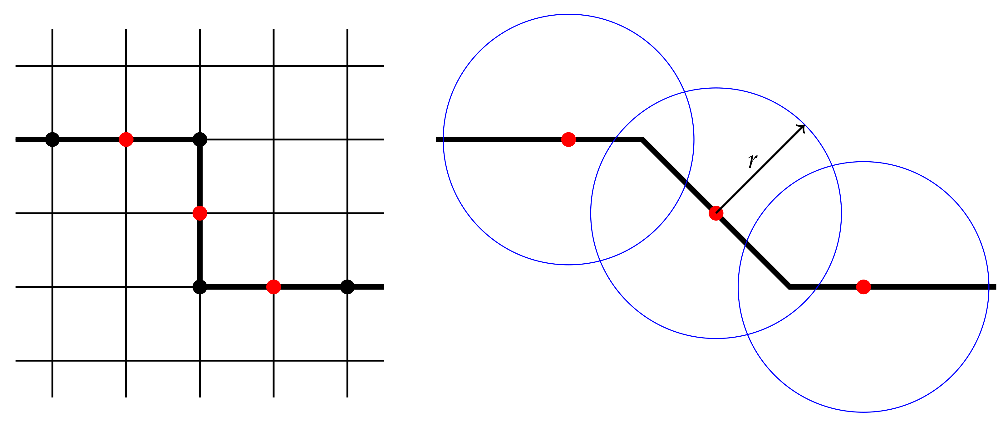
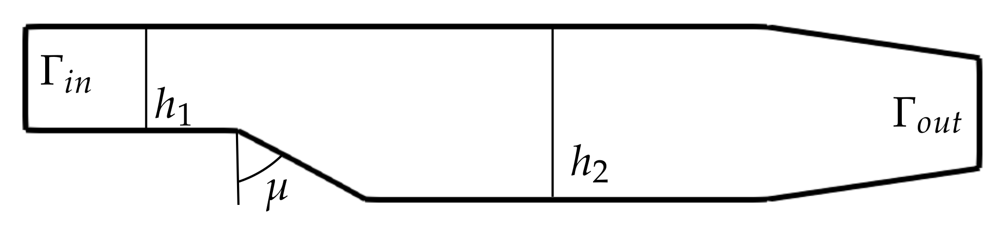
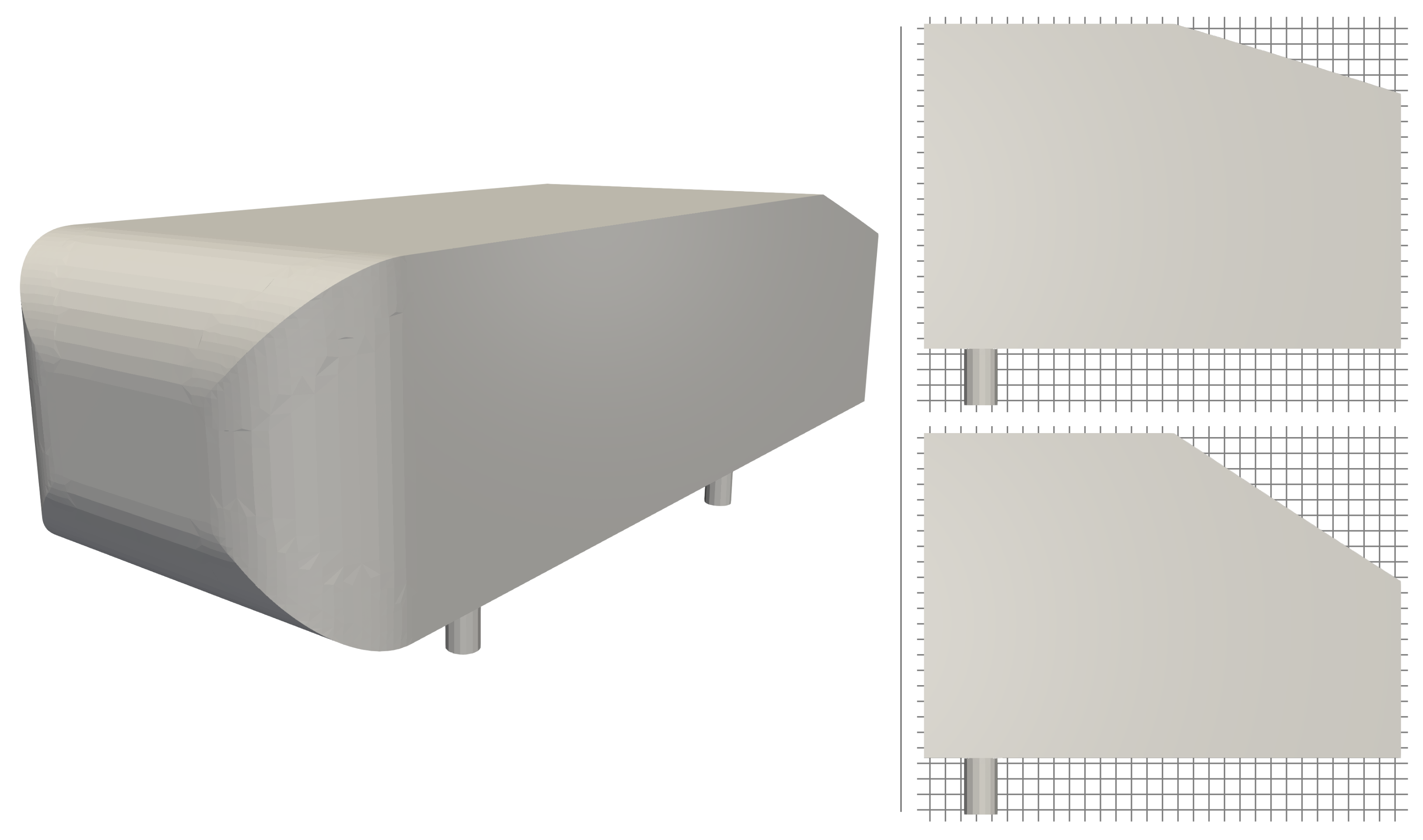
Select the control points in the boundaries to be moved and shift their position obeying the fixed motion rule selected for the geometry modification according to the parameter dependent displacement law: they can be either all the points in the boundary or just a fraction of their total amount if the dimension of the mesh is big enough (see Figure 2), since the higher the number of control points, the bigger (and more expensive) the resulting RBF linear problem to be solved;
2.
Calculate all the parameters for the RBF to ensure the interpolation capability of the scheme
δ ( x i b ) = δ ¯ i b , i = 0 N b ω i q ( x i b ) = 0 ,
resulting in the solution of the following linear problem:
Φ P P T 0 ω α = δ ¯ b 0 ,
where Φ R N b × N b contains the evaluations φ x i b x j b ; P R N b × ( d + 1 ) , with spacial dimension d, is filled as 1 x i b for each row; α contains the coefficients for the polynomial q ( x ) ; and δ ¯ b are the displacements for the control points, known a priori (see [25]);
3.
Evaluate all the remaining points of the grid by applying Equation (4).
A few aspects have to be underlined about the procedure above:
  • Equation (4) is used to move not only the internal points of the grid but also the points located on the moving boundaries that are not selected as control points: even if their displacement could be calculated exactly, changing their position by rigid translation while all the points of the internal mesh are shifted by the use of the RBF may lead to a corrupted grid;
  • Equation (5) requires the resolution of a dense linear problem whose dimension is equal to N b + d + 1 . Thus, the number of control points has to be carefully selected. Fortunately, the resolution of Equation (5) only has to be carried out once, storing all the necessary parameters to be used in the following mesh motions;
  • By the use of this mesh motion strategy, one ends up with meshes having all the same topology, which is an important feature when different geometries have to be compared.

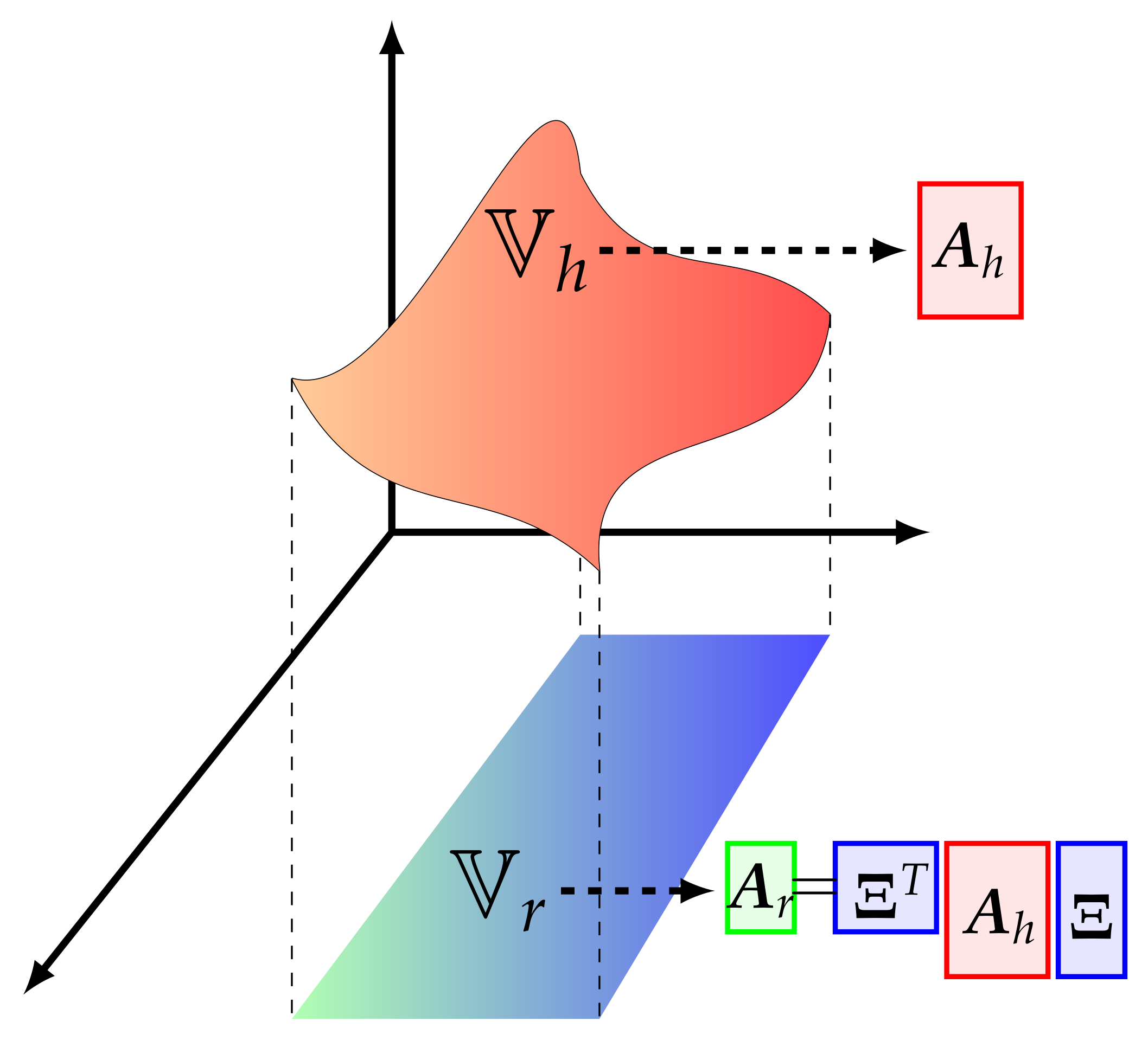
2.3. The Reduced Order Problem

The resolution of Equation (1) for many different values of the parameter may become unaffordable. For this reason, the scope of this work is to find an efficient way to obtain an accurate solution at a lower computational cost, namely a reduced order model (ROM). To pursue this goal, we rely on a POD–Galerkin technique. It consists of computing a certain number of full order solutions s i = s ( μ i ) , where μ i T for i = 1 , , N t , T being the training collection of a certain number N t of parameter values, in order to obtain the maximum amount of information from this costly stage to be employed later on for a cheaper resolution of the problem. These snapshots can be resumed at the end of the resolution all together in a matrix S R N h × N t , so that
S = s 1 1 s 2 1 s N t 1 s 1 N h s 2 N h s N t N h ,
The idea is to perform the ROM resolution that is able to minimize the error E R O M between the obtained realization of the problem and its high fidelity counterpart. In the POD–Galerkin scheme, the reduced order solution can be exploited as follows:
s R O M ( μ ) = j = 1 N r β j ( μ ) ξ j ( x ) ,
where N r N t is a predefined number, namely the dimension of the reduced order solution manifold; β j ( μ ) are some coefficients depending only on the parameter; and ξ j ( x ) are some precalculated orthonormal functions depending only on the position.
The best performing functions ξ j are, in our case, the ones minimizing the L 2 -norm error E R O M between all the reduced order solutions s i R O M , i = 1 , , N t and their high fidelity counterparts:
E R O M = i = 0 N t s i R O M s i L 2 = i = 0 N t j = 1 N r β j ξ j s i L 2 .
Using a proper orthogonal decomposition (POD) strategy, the required basis functions are obtained through the resolution of the following eigenproblem, obtained with the method of snapshots:
C V = V λ ,
where C R N t × N t is the correlation matrix between all the different training solutions, V R N t × N t is the matrix containing the eigenvectors, and λ R N t × N t is the matrix where eigenvalues are located on the diagonal. All the elements of C are composed by the L 2 inner products of all the possible couples of truth solutions s i and s j . Of course, the choice of a POD procedure for the creation of the modal basis functions is not the only possible one (see, e.g., [26,27,28]).
What may be confusing about this last computation is the fact that the L 2 norm is not well defined since all the realizations are obtained for different parameter values and, thus, for different domains. In this work, we overtake this problem by exploiting the fact that all the meshes have the same topology. It is then possible to define a mid-configuration by the mesh motion obtained through a specific parameter μ m i d resulting from:
μ m i d = 1 N t i = 1 N t μ i for μ i T .
In our case, we use equispaced offline parameters to compose T , leading to only μ m i d = μ 1 + μ N t 2 .
The correlation matrix can then be easily assembled as
C i j = s i T M m i d s j ,
M m i d being the mass matrix defined for Ω ( μ m i d ) .
Finally, the POD basis functions are obtained as a linear combination of the training solutions as follows:
ξ i ( x ) = 1 N t j = 1 N t V j i s j ( x ) .
All the basis functions can be collected into a single matrix:
Ξ = ξ 1 , , ξ N r R N h × N r .
It is used to project the original problem onto the reduced subspace so that the final system dimension is only N r . Supposing N r N h , this procedure leads to a problem requiring a computational cost that is much lower with respect to the high fidelity one (see Figure 3).
Many different methods can be chosen to solve the reduced problem. For example, the whole system in Equation (1) can be assembled and projected in a monolitic approach, or the equations can be treated one at a time in an iterative procedure. As we will see in Section 2.4, in this work, we decided to deal with a segregated approach. This means that the momentum predictor and pressure correction steps are iterated until convergence is reached. Since the solution fields during these iterations vary a lot, from the first attempt for the variables to the last resolution, the information contained in the converged snapshots is not sufficient to ensure the correct reduced reconstruction of the path to the global minimum for Equation (1).
To overtake this issue, the idea proposed here is to enrich the set of snapshots for the matrix in Equation (6) by the use of some intermediate snapshots that are stored during the iterations of the full order problem, as shown in Figure 4. The matrix we obtain is
S = s 1 1 , s 1 2 , , s 1 , , s N t 1 , s N t 2 , , s N t .
This procedure, of course, somehow pollutes the physical content of the resulting POD basis functions, since the intermediate step solution’s physical meaning is almost negligible, but the real gain of this procedure is to ensure a better convergence for the ROM algorithm.

2.4. The Reduced Order SIMPLE Algorithm

We present here a new strategy for the resolution of the reduced problem: since for the full order solutions we rely on a segregated pressure based SIMPLE algorithm, the application of a monolithic approach for what concerns the online phase would lead to an inconsistency. In fact, the decoupling of the equations into the system reported in Equation (1) requires a slight modification of their form. For this reason, we developed a reduced order SIMPLE algorithm, based on the full order one, that simulates the high fidelity behaviour for what concerns the convergence to the final solution, utilizing projection-based techniques. In the following Algorithm 1, we present the main steps for the implementation of this algorithm. For the interested reader, its laminar counterpart can be analyzed in more detail in [16]. Turbulence in this algorithm is treated, as it can be done for the whole SIMPLE family of algorithms, by the addition of an extra turbulent viscosity ν t (see [13]).
Let us introduce here the snapshot matrices containing the full order solutions of Equation (1):
S p = p ¯ 1 , , p ¯ N s R N h × N s , S u = u ¯ 1 , , u ¯ N s R ( d N h ) × N s ,
where d is the space dimension of the problem, and N s is the number of realizations equal to the number of provided training parameter values.
For the application of a projection-based reduction procedure of Equation (1), two different sets of basis functions have to be provided for pressure and velocity, respectively. This means that the procedure we exposed in Section 2.3 has to be carried out for both S p and S u . Reduced pressure p ¯ r and reduced velocity u ¯ r can then be written as:
p ¯ r = i = 0 N p b i θ i = Θ T b ,
u ¯ r = i = 0 N u a i ψ i = Ψ T a ,
where N p N s and N u N s are the selected number of modal basis functions chosen to reconstruct pressure and velocity manifolds V p and V u , respectively, so that p ¯ r V p = s p a n { θ 1 , θ N p } and u ¯ r V u = s p a n { ψ 1 , ψ N u } , θ i being the POD basis for pressure and ψ i the POD basis for velocity. Matrices Θ and Ψ contain the modal basis functions for pressure and velocity.
Algorithm 1: The Reduced Order SIMPLE algorithm
     Input: first attempt reduced pressure and velocity coefficients b and a ; modal basis functions matrices for pressure and velocity Θ and Ψ
     Output: reduced pressure and velocity fields p ¯ r and u ¯ r
1:
From b and a , reconstruct reduced fields p ¯ and u ¯ :
p ¯ = Θ T b , u ¯ = Ψ T a ;
2:
Evaluate the eddy viscosity field ν t ;
3:
Momentum predictor step: assemble the momentum equation, project and solve it to obtain a new reduced velocity coefficients a :
( ψ i , A u ¯ H ( u ¯ ) + p ¯ ) L 2 ( Ω ) = 0 ;
4:
Reconstruct the new reduced velocity u ¯ and calculate the off-diagonal component H ( u ¯ ) ;
5:
Pressure correction step: project pressure equation to get new reduced pressure coefficients b :
( θ i , · [ A 1 p ¯ ] · [ A 1 H ( u ¯ ) ] ) L 2 ( Ω ) = 0 ;
Then, correct the velocity explicitly after having reconstructed the new pressure p ¯ ;
6:
Relax the pressure field and the velocity equation with the prescribed under-relaxation factors α p and α u , respectively. The under-relaxed fields are called p ¯ u r and u ¯ u r ;
7:
if convergence then
8:
     u ¯ r = u ¯ u r and p ¯ = p ¯ u r ;
9:
else
10:
    Assemble the conservative face fluxes F i j :
F i j = u ¯ i j · S i j ;
11:
    set u ¯ = u ¯ u r and p ¯ = p ¯ u r ;
12:
    iterate from step 1.
13:
end if
Fluid flows projection-based ROMs usually require being stabilized in some way (see, e.g., [29,30,31]). For Navier–Stokes problems in particular, the use of stable snapshots does not guarantee the Ladyzhenskaya–Brezzi–Babushka condition fulfilment for the saddle-point problem (see [32]). The accuracy in the pressure field is of high relevance for many different configurations (see [33]). In this case, the application of a segregated approach, also at the reduced level, leads to the complete unnecessity of extra stabilization.
In step number 2 of Algorithm 1, no explanation is provided on how to evaluate the eddy viscosity ν t . This is a crucial point of the whole procedure and requires a deeper analysis that we provide for the reader in Section 2.5.

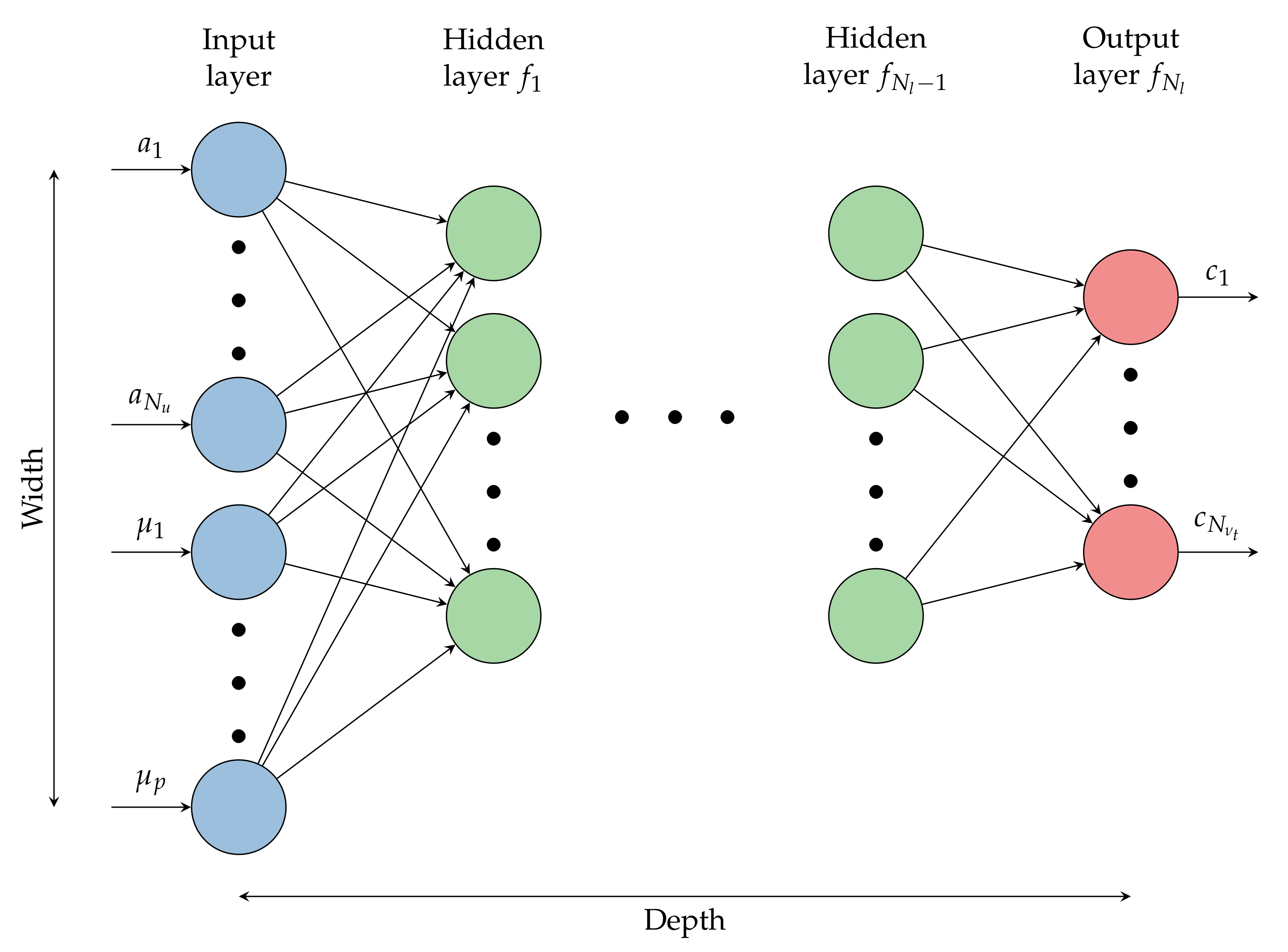
2.5. Neural Network Eddy Viscosity Evaluation

Different possibilities are available for the closure of turbulent problems (see [34]); to make the ROM independent from the chosen turbulence model in the full order model (FOM), different approaches are eligible (see, e.g., [15,35]). In this case, a data-driven approach is employed for the eddy viscosity ν t . Similar to velocity and pressure, first, the reduced eddy viscosity ν t ¯ r is computed via POD on the snapshot matrix S ν t R N h × N s :
ν t ¯ r = i = 0 N ν t c i ζ i = Z T c ,
where ζ i and c i are the POD modes and coefficients for eddy viscosity, respectively, and N ν t N s denotes the selected number of modes to reconstruct the eddy viscosity.
In contrast to the POD coefficients of velocity and pressure, which are obtained by projecting the full order problem onto the respective POD modes and subsequently solving the reduced order problem, the POD coefficients for the eddy viscosity are modelled via a multilayer feedforward neural network. This neural network takes as the input the POD coefficients for velocity a and the corresponding geometrical parameter values μ and maps them to the POD coefficients of the turbulent viscosity c ˜ (tilde denotes a prediction from the neural network) as the output (Figure 5).
Subsequently, the basics of multilayer feedforward neural networks and their training process are briefly reviewed; for a comprehensive description, we refer to Goodfellow et al. [36]. The input to the neural network is commonly denoted as x and for our application reads
x = a 1 a N u μ 1 μ p R ( N u + p ) .
The choice of what to use for the input is supported by the fact that the dependency of the eddy viscosity field on the velocity field is well known because of the way the RANS equations are constructed, while the dependency on the geometric parameters helps in the accuracy of the network. The mapping from this input vector to the coefficients for the eddy viscosity c ˜ is learned by the multilayer neural network via N l fully connected layers:
c ˜ = f N l ( f N l 1 ( f 1 ( W 1 x + b 1 ) ) ) ,
where layer i ( i = 1 , , N l ) performs an affine transformation of its input (specified by the trainable weight matrix W i and bias b i ) that is subsequently passed through the (linear or nonlinear) element-wise activation function f i .
To train the weights θ = { W i , b i } i = 1 N l in supervised learning, the empirical risk over the training data J is minimized:
J ( θ ) = E x p ˜ d a t a L ( c ˜ , c ) = 1 n t r a i n i = 1 n t r a i n L ( c ˜ ( i ) , c ( i ) ) ,
where p ˜ d a t a and n t r a i n denote the empirical distribution of the training data and the number of training samples, respectively; L ( c ˜ , c ) is a per-sample loss metric that describes the discrepancy between target output c (given by training data) and predicted output c ˜ (by neural network).
As a loss function, we use the squared L 2 -loss function (also known as mean squared error), the most common choice for the loss function in regression problems:
L = c c ˜ 2 2 .
Employing this loss function, the objective function J is minimized using the Adam [37] optimizer with minibatching, and the required gradients of the parameters with respect to the loss function are calculated via backpropagation [38].
The hyperparameters of the neural network, which are the parameters that are not subject to optimization during training, were tuned for each test case separately by minimizing the loss on a designated validation data set (while the accuracy evaluation of the neural network was finally performed on a third set, referred to as a test set). The hyperparameters subject to tuning were: the height and width of the neural network (i.e., the number of hidden layers and units per hidden layer, cf. Figure 5), the activation functions for each layer, and the learning rate as well as the batch size of the Adam optimizer. For the creation and training of the neural networks, we employed the Python library PyTorch [39].
Remark 1.
In Algorithm 1, prior to the Galerkin projection, due to the nonlinearity, we reconstruct the full order model fields using the reduced coefficients for both the velocity and pressure fields. This fact, also associated with the fact that the ROM code is not as optimized as the OpenFOAM library, results in a reduced order model that has a computational cost which is comparable with the full order model. In order to make the ROM methodology more efficient, it would be required to develop a suitable hyper-reduction technique such as the discrete empirical interpolation [16] method or a similar technique and properly optimize the ROM code.

3. Results

3.1. Academic Test Case

The first test case we propose for checking the effectiveness of the procedure previously described is a classical 2D back step problem where the slope of the step is parametrized and can be varied (see Figure 6).
All the results provided in this paper are obtained by the use of an in-house open source library ITHACA-FV (In real Time Highly Advanced Computational Applications for Finite Volumes) [40], developed in a finite volume environment based on the solver OpenFOAM [41].
The set of equations we want to consider are the ones reported in Equation (1), where g D = 1 , 0 , 0 T , g N = 0 , the eddy viscosity ν t is obtained by the resolution of a k ϵ turbulence model, and ν = 1 × 10 3 .
With reference to Figure 6, the height of the duct at the inlet, namely h 1 , is equal to one, while it is equal to 1.7 in the middle of the channel, namely h 2 . The domain is divided into a 14 × 10 3 hexahedral cell mesh. The mesh motion is carried out by the use of a radial basis function approach, as explained in Section 2.2.
The Reynolds number characterizing the dynamics of the problem can be evaluated, taking into account both the fluid properties together with geometrical aspects as
R e = u ¯ h 2 ν = 1.7 × 10 3 .
Since the range for the Reynolds number we are working with is on the border line between laminar and turbulent flows, we are forced to consider a turbulence closure model.
For the offline phase, we selected 50 equispaced values of the parameter μ [ 0 , 75 ] . Those values of the angle of the step were used to solve 50 different full order problems in order to construct the snapshots matrix.
By applying a POD procedure, we can obtain the modal basis functions we need to project the equations.
By analysing Figure 7, we can notice that at least 25 modes have to be selected for ν t in order to catch the main part of the information contained in the offline snapshots. Regarding pressure and velocity manifolds, here, they are projected and then reconstructed using 35 basis functions.
Thus, a neural network has been constructed for the eddy viscosity approximation at every reduced SIMPLE algorithm step as explained in Section 2.4.
The neural network employed here is composed by:
  • An input layer, whose dimension is equal to the dimension of the reduced velocity, i.e., 35, plus one for the parameter;
  • Two hidden layers of dimensions 256 and 64 respectively;
  • An output layer of dimension 25 for the reduced eddy viscosity coefficients.
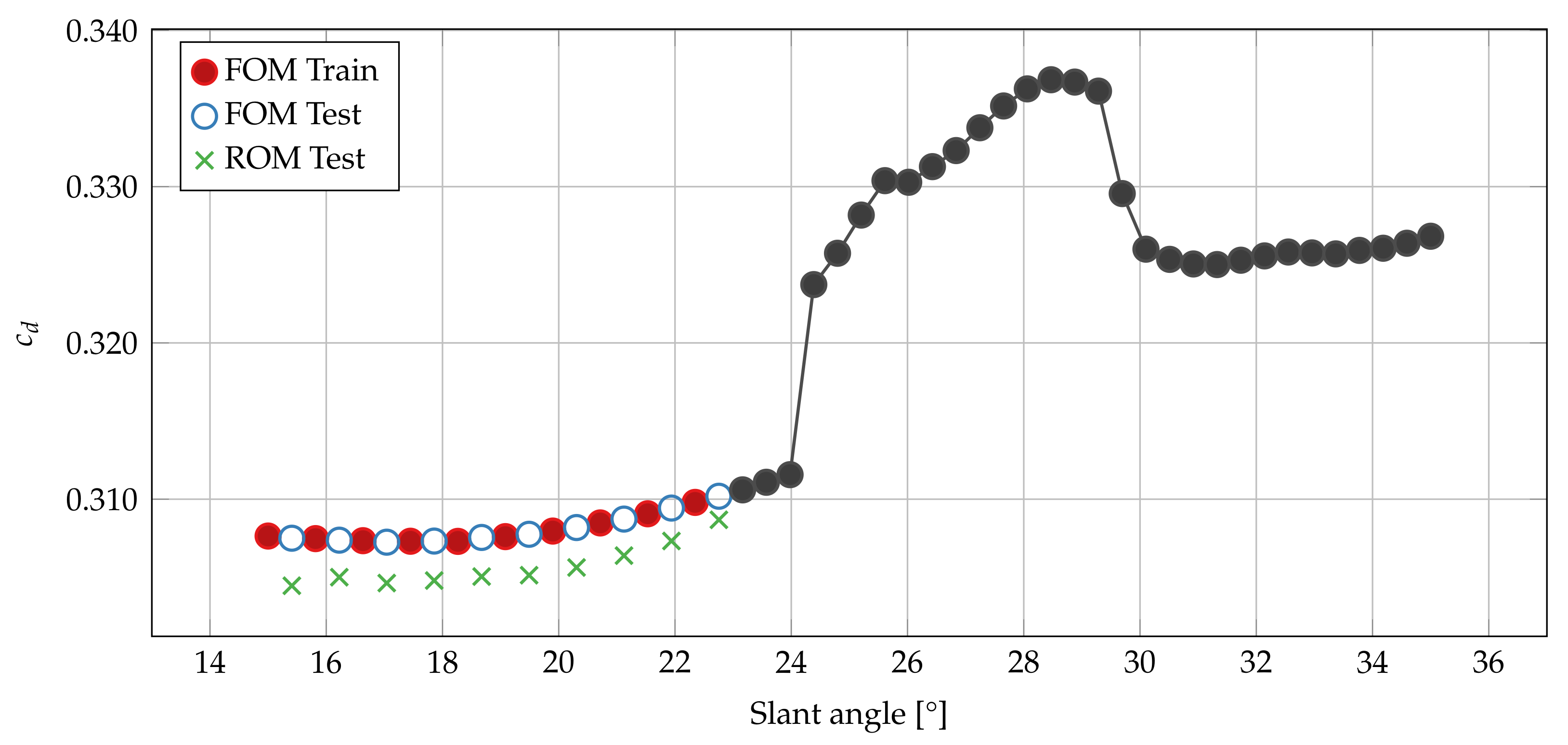
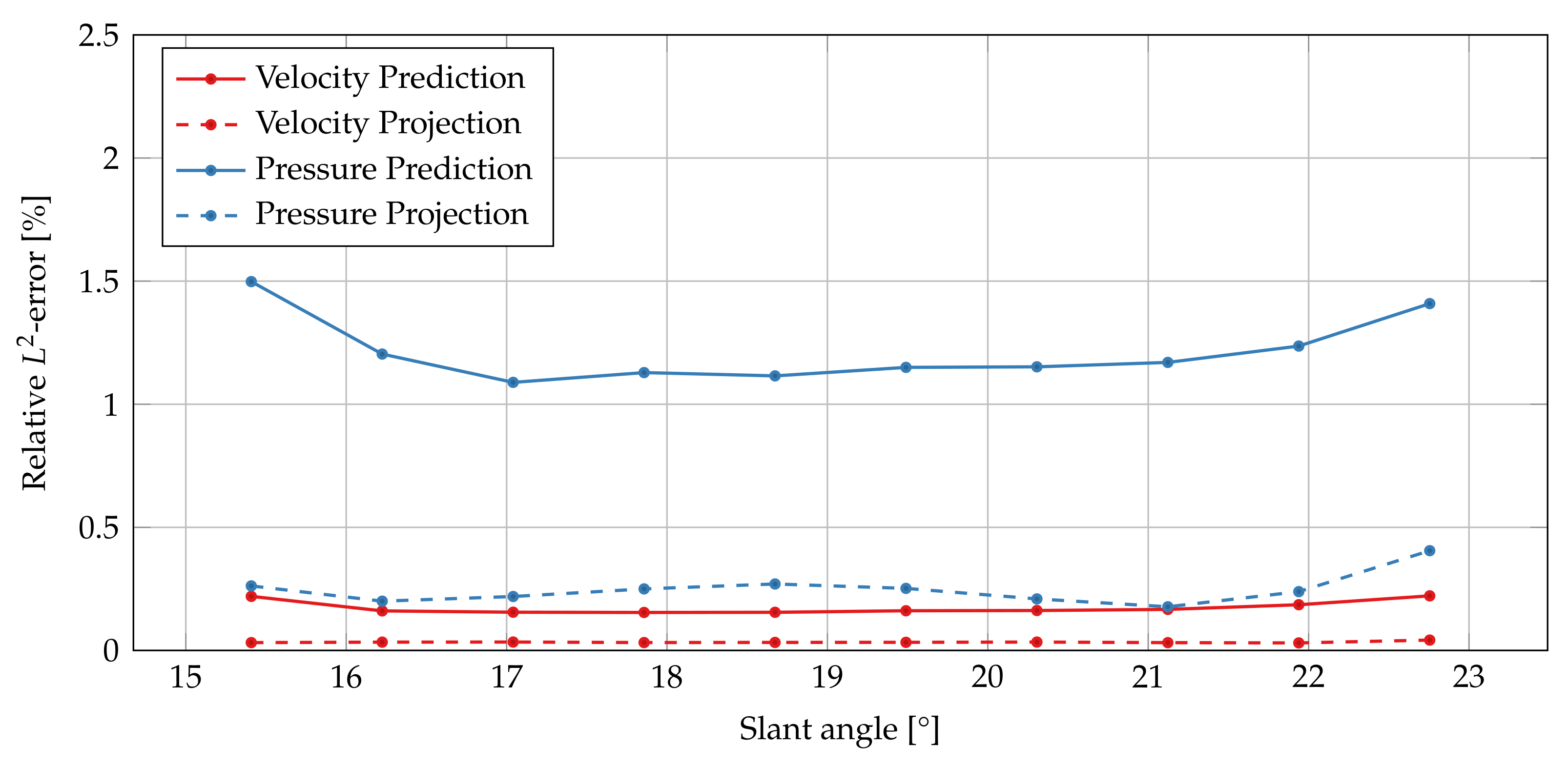
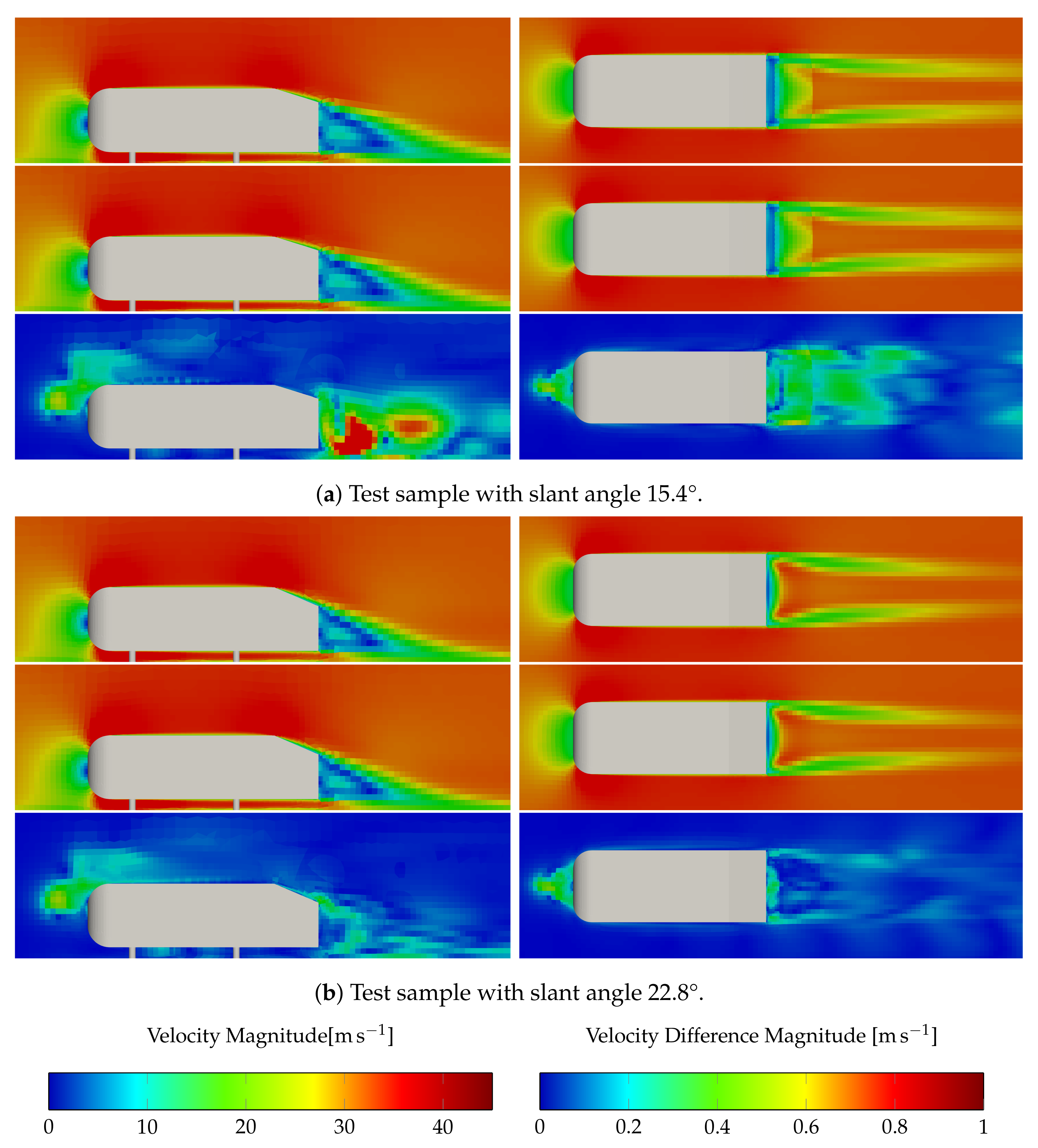
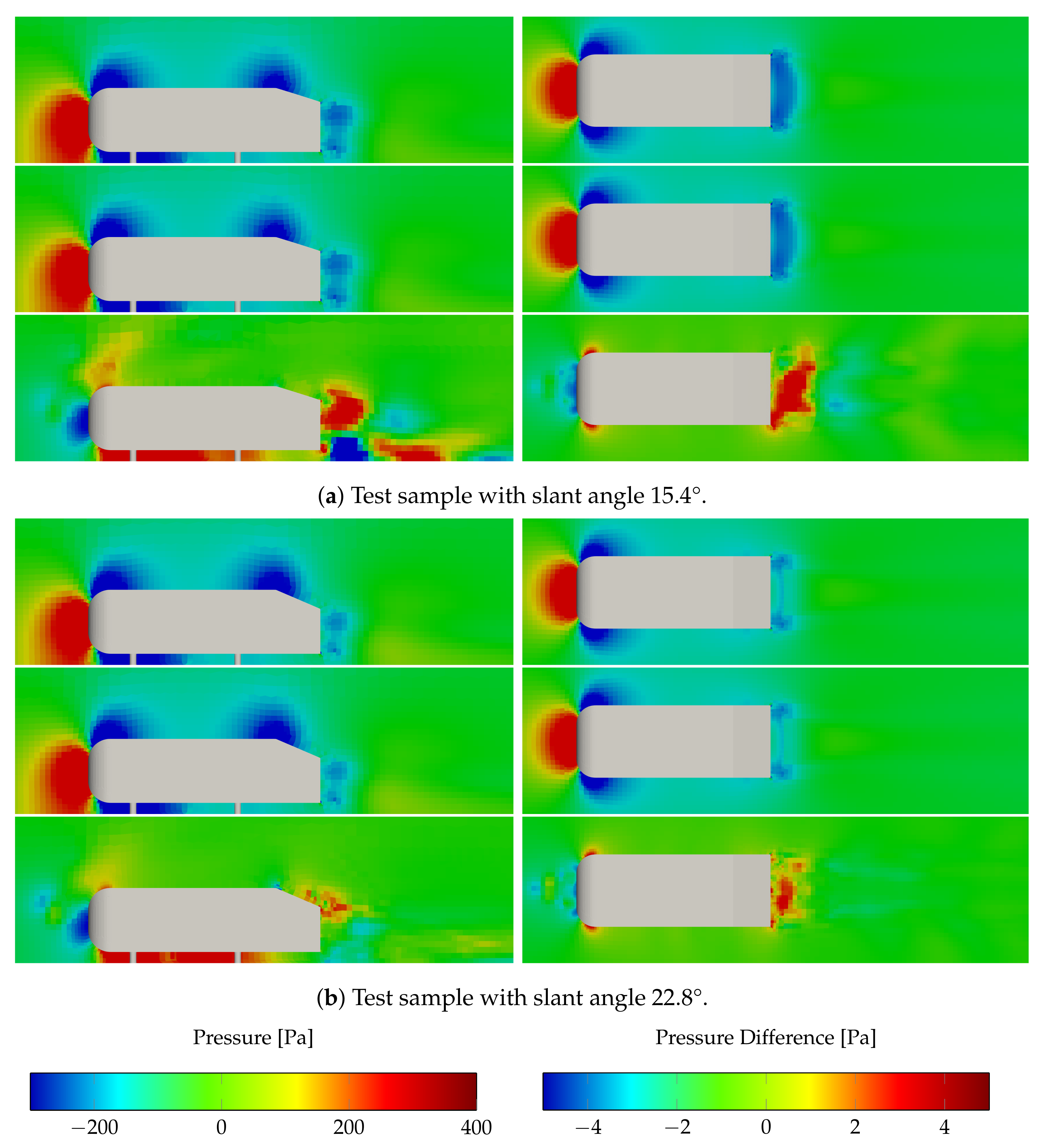
The net is a fully connected one. Moreover, the neurons of the hidden layers are characterized by the employment of ReLU activation functions. For the training procedure, the Adam optimizer has been selected, and 10 4 epochs have been fixed.
The training set is composed by both the intermediate and final solutions obtained during the offline phase, randomly selected. To control the training procedure, a test set has also been selected: 10 totally random new parameter values have been chosen and their related full solutions have been calculated, saving both final and intermediate steps, coherently with the offline snapshots used for training.
Looking at Figure 8, it can be noticed that there is a nice agreement between train and test loss functions. This is a good indicator for the extrapolation capability of the net.
In Figure 9, Figure 10 and Figure 11, we show the comparisons between full order model (FOM) and ROM solutions for velocity, pressure, and eddy viscosity. Two random angles have been selected to show the behaviour of the model for both a very low parameter value and a very high one.
As it may be noticed, the reconstruction of the reduced order model is very accurate, and the errors are pretty low. The main differences between the high fidelity and the reduced solutions are present for high values of the parameter. This is to be addressed by the fact that the mesh is really distorted for those cases, and the good orthogonality properties of the original mesh are lost. In any case, the model is able to tackle the full order solution and can predict in a consistent way the correct solution.
As proof of what has just been said, we show in Figure 12 the trend of the L 2 norm relative errors while varying the dimension of the reduced manifolds for velocity and pressure at the same time. The values presented in this plot are the mean relative errors between 10 randomly chosen parameters for the online phase.

3.2. Ahmed Body

As the second test case, we chose an automotive external aerodynamic one: the Ahmed body [42]. The Ahmed body is a generic vehicle: the flow around the back of this bluff body contains the main flow structures that are also encountered for real-life vehicles. We defined one geometrical parameter—the slant angle—using RBF mesh morphing (see Section 2.2). Figure 13 shows the Ahmed body and illustrates the covered design space by the slant angle parameter. As shown in experiments by Ahmed et al. [42] and Lienhart et al. [43], three main flow regimes occur based on the slant angle: (1) below approximately 12 ° , the flow remains attached over the slant; (2) between 12 ° and 30 ° , forming c-pillar vortices as well as recirculation regions at the top and base increases drag; and (3) at approximately 30 ° , the flow fully separates off the slant, thus leading to a sudden drag decrease.
The common practice for automotive external aerodynamics is the detached eddy simulation (DES) [44]; therein, the method of choice is the Spalart–Allmaras for the turbulence model. As we intend to extend the RANS-based ROM presented in this article to DES in future work, we already employ the Spalart–Allmaras turbulence model for the RANS computations to resemble the operational simulation process.
At this stage, the study is restricted to the initial part of a single flow regime ranging from 15 ° to 23 ° , which already constitutes a demanding task. We sampled this parameter range uniformly with 20 RANS simulations using OpenFOAM®; these 20 simulations were decomposed into 10 for training (offline phase) the ROM and 10 for assessing its accuracy (online phase). The inlet velocity for the simulations was set to 40 m s 1 , thus resulting in a Reynolds number of ≈ 2.8 × 10 6 based on the model length. Each mesh was created with SnappyHexMesh® and contained about 200,000 cells. While from a CFD perspective, the meshes are very coarse, they constitute a challenge for the ROM, and they are considerably larger compared with those of the academic test case ( 35 × 10 4 vs. 14 × 10 3 cells). We chose this rather coarse mesh as we aimed to at least qualitatively reproduce the experiments. Figure 14 shows the corresponding cumulated eigenvalues for velocity, pressure, and eddy viscosity. For the upcoming investigations, we chose to keep 30 POD modes for all three fields.
As shown in Figure 15, we reproduced the three typical flow regimes encountered in the experiments. We emphasize that to assess the accuracy of our ROM, we compare the flow field predictions with respect to the FOM (and not the experiments). If a higher accuracy of the ROM with respect to the experiments is desired, this can be achieved by increasing the FOM accuracy, e.g., by refining the CFD mesh.
We saved every 20th of the total 2000 iterations as snapshots (velocity, pressure, and eddy viscosity fields), resulting in 100 snapshots per simulated slant angle. Each simulation took about 3 min on 16 CPU cores.
After assembling the snapshot matrices with the intermediate as well as the converged iteration of the FOM simulations, we decomposed those matrices into modes and coefficients via POD.
As described in Section 2.5, the POD coefficients of the eddy viscosity are modelled via a neural network. For the present test case, the input of this neural network—for each of the 1000 training samples (10 angle values times 100 saved iterations per angle)—is given by the 30 POD coefficients of velocity and, additionally, the slant angle. The optimized neural network architecture consists of two hidden layers with 128 units each, Tanh activation functions, and a learning rate of 0.001 for the Adam optimizer, thereby using a batch size of 128; the training was terminated after 10,000 epochs.
Similar to the academic test case, we assessed the model accuracy on the test dataset (the 1000 samples corresponding to the 10 test geometries) and found that the model generalizes well to unseen data.
With the trained neural network for the eddy viscosity, we are able to solve the reduced order problem for test geometries, i.e., slant angle configurations not present in the training data. Subsequently, we evaluate the ROM accuracy quantitatively and qualitatively by comparing ROM and FOM results for the 10 test geometries. For the quantitative analysis, we (1) compare the drag coefficients and (2) compare the relative L 2 -errors between the velocity and pressure fields from ROM and FOM. For the qualitative comparison, we compare the velocity and pressure fields on two slices through the computational domain for two chosen test geometries. For one of those test geometries, we additionally inspect the residual drop while solving the reduced order problem.
We start the accuracy assessment with the drag coefficient, the major quantity of interest in the development of vehicle aerodynamics. As the drag coefficient of the ROM is obtained by integrating the pressure and wall shear stress over the vehicle surface, this investigation also allows us to implicitly assess the accuracy of surface field predictions for those fields. Figure 15 shows the drag coefficient c d over the slant angle for the conducted 20 FOM simulations and indicates the even distribution in the parameter space of the geometries used for training and testing.
The minimum and maximum absolute errors of the ROM are 1.5 (test sample at slant angle 22.8 ° ) and 3.0 ( 15.4 ° ) drag counts, respectively, while the mean error over all 10 test samples amounts to 2.4 drag counts. The drag coefficient in automotive vehicle aerodynamics is dominated by the pressure contribution (approximately 85% pressure and 15% viscous contribution for the present test case); accordingly, we found that the error in surface pressure between ROM and FOM accounts for the majority of the total error in the drag coefficient prediction. Therefore, the visible systematic offset between ROM and FOM for the drag coefficient can probably be reduced by improving the pressure field prediction, which is investigated next.
Figure 16 shows the relative L 2 -errors between ROM prediction and FOM (solid lines) for velocity and pressure. As for the drag coefficient, the highest errors for both fields are encountered for the test sample with 15.4 ° slant angle. The errors for pressure are one magnitude higher compared with those for velocity. Additionally, the projection errors—the lower bounds for the ROM errors—are shown (dashed lines). While for the velocity, a ROM prediction error close to the projection error is achieved, there is still room for improvement in the case of pressure (vertical distance between blue solid and dashed lines). In the image we denote with prediction the relative L 2 -error between the results obtained with the FOM (i.e., OpenFOAM simulations) and the results obtained with the ROM (i.e., using Algorithm 1). With the term projection, we denote the relative L 2 -error between the FOM solutions and the projection of the FOM solutions onto the space spanned by the POD modes. These results, being the best representation of the solution fields, given the POD space, give us reference values for the best accuracy that the ROM can achieve.
Finally, Figure 17 and Figure 18 compare the FOM and ROM fields qualitatively for velocity and pressure, respectively. We chose the test samples with the lowest and highest slant angle for this visual comparison.
For velocity and pressure, ROM and FOM results are in good agreement on both presented slices. In accordance with the quantitative results, for both fields, the errors for slant angle 15.4 ° are higher compared with those at 22.8 ° .
As the parametrization alters the vehicle geometry exclusively at the rear end, the main flow field variations are expected to occur in the wake area of the vehicle; accordingly, for velocity, the highest ROM errors are visible in this region. Additionally, smaller regions at the top of the front end exhibit higher errors for both test samples.
For the pressure, the regions of highest errors are scattered around the vehicle surface. Besides the wake region, in particular, below the vehicle underbody, high errors occur. The deficiencies of the pressure prediction of the ROM near the surface likely result in relatively high errors for the drag coefficients, which is a topic of improvement for future work.
For the test geometry with the lowest slant angle, we also inspect the residuals while solving the reduced order problem. The residuals drop approximately one and three orders of magnitude for pressure and velocity, respectively. Even though the residual computation differs for the FOM, forbidding a direct comparison of FOM and ROM residuals, the FOM residuals also exhibit a rather small drop of three to four orders of magnitude. This small drop of the residual even at the FOM level can be accounted for by the unsteady flow around the stilts of the Ahmed body (comparable to vortex shedding around cylinders); as we simulate the problem with the steady RANS approach, rather high and oscillating residuals in the underbody region remain even after solver “convergence”. As mentioned earlier, future efforts include the transition from steady RANS to unsteady DES, which will, e.g., inherently model the unsteady flow around the stilts more accurately.

4. Discussion

In this paper, we presented a new approach based on a technique that combines a classical projection-based method concerning both the momentum equation and the incompressibility constraint with a data-driven procedure regarding the eddy viscosity closure.
This choice revealed a wide applicability and flexibility since the turbulence model selected for the offline phase does not affect the computations in any way during the online phase. Moreover, the reconstruction of the eddy viscosity field is very accurate, as shown in Section 3.1.
The reduced SIMPLE algorithm we presented here in Section 2.4, taking advantage of the coupling between the accuracy of projection-based methods and the versatility of neural networks, was shown to guarantee good approximations in widely different fluid dynamics test cases. Moreover, the idea of collecting converged fields together with middle iteration solutions ensures good convergence properties without showing relevant errors due to the physical information pollution of the modal basis functions, as explained in Section 2.3.
Finally, the choice of relying on an RBF approach for the mesh motion was demonstrated to be effective while preserving a good shape of the modified mesh.
Concerning the efficiency of the online phase of the problem, some improvements are still required, and a natural step forward for this kind of application would be the development of hyper reduction techniques for the reduced operators. This task could be also entrusted to neural network approaches, attempting to approximate the reduced operators by the evaluation, e.g., of an autoencoder. In any case, the scope of this article was not focused on highly efficient hyper reduction techniques. Thus, even if in this procedure, we are still relying on reconstructed full-dimension reduced order fields to assemble the equations, the results are, in any case, also appreciable in terms of the time consumed.

Author Contributions

Conceptualization, G.S. and G.R.; methodology, All Authors; software M.Z., M.M. and G.S.; validation M.Z., M.M., C.O. and G.S.; formal analysis, M.Z., M.M. and G.S.; investigation, M.Z., M.M.; resources G.R. and C.O.; data curation, M.Z., M.M.; writing—original draft preparation, M.Z., M.M. and G.S.; writing—review and editing, All Authors.; visualization, M.Z. and M.M.; supervision, G.R., C.O. and G.S.; project administration, G.R. and C.O.; funding acquisition, G.R. and C.O. All authors have read and agreed to the published version of the manuscript.

Funding

European Commission H2020 ARIA (Accurate ROMs for Industrial Applications) project G.A. 872442, MIUR (Italian Ministry for Education University and Research) FARE-X-AROMA-CFD project and PRIN “Numerical Analysis for Full and Reduced Order Methods for Partial Differential Equations” (NA-FROM-PDEs) project, European Research Council Consolidator Grant Advanced Reduced Order Methods with Applications in Computational Fluid Dynamics project G.A. 681447, H2020-ERC COG 2015 AROMA-CFD.

Data Availability Statement

The data presented in this study are available on request from the corresponding author. The code used to generate the numerical results is publicly available on github https://github.com/mathLab/ITHACA-FV.

Acknowledgments

We acknowledge the support by the European Commission H2020 ARIA (Accurate ROMs for Industrial Applications) project, by MIUR (Italian Ministry for Education University and Research) FARE-X-AROMA-CFD project and PRIN “Numerical Analysis for Full and Reduced Order Methods for Partial Differential Equations” (NA-FROM-PDEs) project, and by the European Research Council Consolidator Grant Advanced Reduced Order Methods with Applications in Computational Fluid Dynamics-GA 681447, H2020-ERC COG 2015 AROMA-CFD. The main computations in this work were carried out by the usage of ITHACA-FV [40], a library maintained at SISSA mathLab, an implementation in OpenFOAM [41] for reduced order modelling techniques. Its developers and contributors are acknowledged.

Conflicts of Interest

The authors declare no conflict of interest.

References

  1. Benner, P. Model Order Reduction: Volume 1 System and Data-Driven Methods and Algorithms; De Gruyter: Berlin, Germany, 2020. [Google Scholar] [CrossRef]
  2. Benner, P.; Schilders, W.; Grivet-Talocia, S.; Quarteroni, A.; Rozza, G.; Silveira, L.M. Model Order Reduction: Volume 2 Snapshot-Based Methods and Algorithms; De Gruyter: Berlin, Germany, 2020. [Google Scholar] [CrossRef]
  3. Iapichino, L.; Quarteroni, A.; Rozza, G.; Volkwein, S. Reduced basis method for the Stokes equations in decomposable parametrized domains using greedy optimization. In European Consortium for Mathematics in Industry; Springer: Berlin/Heidelberg, Germany, 2014; pp. 647–654. [Google Scholar]
  4. Salmoiraghi, F.; Scardigli, A.; Telib, H.; Rozza, G. Free-form deformation, mesh morphing and reduced-order methods: Enablers for efficient aerodynamic shape optimisation. Int. J. Comput. Fluid Dyn. 2018, 32, 233–247. [Google Scholar] [CrossRef]
  5. Stabile, G.; Rozza, G. Finite volume POD-Galerkin stabilised reduced order methods for the parametrised incompressible Navier–Stokes equations. Comput. Fluids 2018, 173, 273–284. [Google Scholar] [CrossRef] [Green Version]
  6. Tsiolakis, V.; Giacomini, M.; Sevilla, R.; Othmer, C.; Huerta, A. Nonintrusive proper generalised decomposition for parametrised incompressible flow problems in OpenFOAM. Comput. Phys. Commun. 2020, 249, 107013. [Google Scholar] [CrossRef] [Green Version]
  7. Lee, K.; Carlberg, K.T. Model reduction of dynamical systems on nonlinear manifolds using deep convolutional autoencoders. J. Comput. Phys. 2020, 404, 108973. [Google Scholar] [CrossRef] [Green Version]
  8. Kim, Y.; Choi, Y.; Widemann, D.; Zohdi, T. Efficient nonlinear manifold reduced order model. arXiv 2020, arXiv:2011.07727. [Google Scholar]
  9. Benner, P.; Gugercin, S.; Willcox, K. A Survey of Projection-Based Model Reduction Methods for Parametric Dynamical Systems. SIAM Rev. 2015, 57, 483–531. [Google Scholar] [CrossRef]
  10. Brunton, S.L.; Kutz, J.N. Data-Driven Science and Engineering; Cambridge University Press: Cambridge, UK; New York, NY, USA, 2019. [Google Scholar] [CrossRef] [Green Version]
  11. Pope, S.B. Turbulent Flows; Cambridge University Press: Cambridge, UK, 2000. [Google Scholar]
  12. Berselli, L.C. Mathematics of Large Eddy Simulation of Turbulent Flows; Springer: Berlin, Germany, 2006. [Google Scholar]
  13. Wilcox, D.C. Turbulence Modeling for CFD; DCW Industries: La Canada, CA, USA, 1998; Volume 2. [Google Scholar]
  14. Hijazi, S.; Stabile, G.; Mola, A.; Rozza, G. Data-Driven POD–Galerkin reduced order model for turbulent flows. J. Comput. Phys. 2020, 416, 109513. [Google Scholar] [CrossRef]
  15. Georgaka, S.; Stabile, G.; Star, K.; Rozza, G.; Bluck, M.J. A hybrid reduced order method for modelling turbulent heat transfer problems. Comput. Fluids 2020, 208, 104615. [Google Scholar] [CrossRef]
  16. Stabile, G.; Zancanaro, M.; Rozza, G. Efficient Geometrical parametrization for finite-volume based reduced order methods. Int. J. Numer. Methods Eng. 2020, 121, 2655–2682. [Google Scholar] [CrossRef]
  17. Moukalled, F.; Mangani, L.; Darwish, M. The Finite Volume Method in Computational Fluid Dynamics; Springer: Berlin/Heidelberg, Germany, 2016; Volume 113. [Google Scholar]
  18. Donea, J.; Huerta, A. Finite Element Methods for Flow Problems; John Wiley & Sons: Hoboken, NJ, USA, 2003. [Google Scholar]
  19. Busto, S.; Stabile, G.; Rozza, G.; Vázquez-Cendón, M.E. POD–Galerkin reduced order methods for combined Navier–Stokes transport equations based on a hybrid FV-FE solver. Comput. Math. Appl. 2020, 79, 256–273. [Google Scholar] [CrossRef] [Green Version]
  20. Jasak, H. Error Analysis and Estimation for the Finite Volume Method with Applications to Fluid Flows. Ph.D. Thesis, Imperial College London, London, UK, 1996. [Google Scholar]
  21. Hirsch, C. Numerical Computation of Internal and External Flows: The Fundamentals of Computational Fluid Dynamics; Butterworth-Heinemann: Oxford, UK, 2007. [Google Scholar]
  22. Caiazzo, A.; Iliescu, T.; John, V.; Schyschlowa, S. A numerical investigation of velocity–pressure reduced order models for incompressible flows. J. Comput. Phys. 2014, 259, 598–616. [Google Scholar] [CrossRef]
  23. Drohmann, M.; Haasdonk, B.; Ohlberger, M. Reduced basis method for finite volume approximation of evolution equations on parametrized geometries. In Proceedings of the ALGORITMY, Podbanske, Slovakia, 15–20 March 2009; Volume 2008, pp. 111–120. [Google Scholar]
  24. De Boer, A.; Van der Schoot, M.; Bijl, H. Mesh deformation based on radial basis function interpolation. Comput. Struct. 2007, 85, 784–795. [Google Scholar] [CrossRef]
  25. Bos, F.M.; van Oudheusden, B.W.; Bijl, H. Radial basis function based mesh deformation applied to simulation of flow around flapping wings. Comput. Fluids 2013, 79, 167–177. [Google Scholar] [CrossRef]
  26. Dumon, A.; Allery, C.; Ammar, A. Proper general decomposition (PGD) for the resolution of Navier–Stokes equations. J. Comput. Phys. 2011, 230, 1387–1407. [Google Scholar] [CrossRef] [Green Version]
  27. Chinesta, F.; Huerta, A.; Rozza, G.; Willcox, K. Model reduction methods. In Encyclopedia of Computational Mechanics, 2nd ed.; John Wiley & Sons: Chichester, UK; Hoboken, NJ, USA, 2017; pp. 1–36. [Google Scholar]
  28. Hesthaven, J.S.; Rozza, G.; Stamm, B. Certified Reduced Basis Methods for Parametrized Partial Differential Equations; Springer: Berlin/Heidelberg, Germany, 2016; Volume 590. [Google Scholar]
  29. Bergmann, M.; Bruneau, C.H.; Iollo, A. Enablers for robust POD models. J. Comput. Phys. 2009, 228, 516–538. [Google Scholar] [CrossRef] [Green Version]
  30. Iollo, A.; Lanteri, S.; Désidéri, J.A. Stability properties of POD–Galerkin approximations for the compressible Navier–Stokes equations. Theor. Comput. Fluid Dyn. 2000, 13, 377–396. [Google Scholar] [CrossRef] [Green Version]
  31. Azaïez, M.; Rebollo, T.C.; Rubino, S. A cure for instabilities due to advection-dominance in POD solution to advection-diffusion-reaction equations. J. Comput. Phys. 2021, 425, 109916. [Google Scholar] [CrossRef]
  32. Ballarin, F.; Manzoni, A.; Quarteroni, A.; Rozza, G. Supremizer stabilization of POD–Galerkin approximation of parametrized steady incompressible Navier–Stokes equations. Int. J. Numer. Methods Eng. 2015, 102, 1136–1161. [Google Scholar] [CrossRef]
  33. Stabile, G.; Hijazi, S.; Mola, A.; Lorenzi, S.; Rozza, G. Advances in reduced order modelling for CFD: Vortex shedding around a circular cylinder using a POD-Galerkin method. arXiv 2017, arXiv:1701.03424. [Google Scholar]
  34. Wang, Z.; Akhtar, I.; Borggaard, J.; Iliescu, T. Proper orthogonal decomposition closure models for turbulent flows: A numerical comparison. Comput. Methods Appl. Mech. Eng. 2012, 237, 10–26. [Google Scholar] [CrossRef] [Green Version]
  35. Hijazi, S.; Ali, S.; Stabile, G.; Ballarin, F.; Rozza, G. The effort of increasing Reynolds number in projection-based reduced order methods: From laminar to turbulent flows. In Numerical Methods for Flows; Springer: Berlin/Heidelberg, Germany, 2020; pp. 245–264. [Google Scholar]
  36. Goodfellow, I.; Bengio, Y.; Courville, A. Deep Learning; MIT Press: Cambridge, MA, USA, 2016. [Google Scholar]
  37. Kingma, D.; Ba, J. Adam: A Method for Stochastic Optimization. arXiv 2014, arXiv:1412.6980. [Google Scholar]
  38. Rumelhart, D.E.; Hinton, G.E.; Williams, R.J. Learning Representations by Back-Propagating Errors. Nature 1986, 323, 533–536. [Google Scholar] [CrossRef]
  39. Paszke, A.; Gross, S.; Massa, F.; Lerer, A.; Bradbury, J.; Chanan, G.; Killeen, T.; Lin, Z.; Gimelshein, N.; Antiga, L.; et al. PyTorch: An Imperative Style, High-Performance Deep Learning Library. In Advances in Neural Information Processing Systems 32; Wallach, H., Larochelle, H., Beygelzimer, A., d’Alché-Buc, F., Fox, E., Garnett, R., Eds.; Curran Associates, Inc.: Red Hook, NY, USA, 2019; pp. 8024–8035. [Google Scholar]
  40. Stabile, G.; Rozza, G. ITHACA-FV-in Real Time Highly Advanced Computational Applications for Finite Volumes. Available online: http://www.mathlab.sissa.it/ithaca-fv (accessed on 31 March 2021).
  41. OpenFOAM Documentation Website. Available online: https://openfoam.org/ (accessed on 31 March 2021).
  42. Ahmed, S.; Ramm, G.; Faltin, G. Some Salient Features of The Time-Averaged Ground Vehicle Wake; SAE Technical Paper; SAE International: Warrendale, PA, USA, 1984. [Google Scholar] [CrossRef]
  43. Lienhart, H.; Stoots, C.; Becker, S. Flow and Turbulence Structures in the Wake of a Simplified Car Model (Ahmed Model). Notes Numer. Fluid Mech. 2002, 77, 323–330. [Google Scholar] [CrossRef]
  44. Islam, M.; Decker, F.; De Villiers, E.; Jackson, A.; Gines, J.; Grahs, T.; Gitt-Gehrke, A.; Font, J. Application of Detached-Eddy Simulation for Automotive Aerodynamics Development. In SAE World Congress & Exhibition; SAE International: Warrendale, PA, USA, 2009. [Google Scholar] [CrossRef] [Green Version]
Figure 1. Scheme of the relation between two neighbour cells of the tessellation T .
Fluids 06 00296 g001
Figure 2. Scheme of the RBF mesh motion procedure: original mesh on the left and deformed boundary on the right, where red dots represent the control points, while blue circles show the support of the function φ .
Fluids 06 00296 g002
Figure 3. Projection of the full order space V h over the reduced one V r spanned by the basis functions Ξ , where A h and A r are the full order and reduced order matrices related to the considered problem, respectively.
Fluids 06 00296 g003
Figure 4. Scheme of the snapshot selection for every parameter μ i : all red and black dots are collected together to compose the train set. Here, s i i n i t is the first attempt solution, s i j is the j-th iteration solution, and s i f is the final converged snapshot.
Fluids 06 00296 g004
Figure 5. Illustration of a neural network that maps the POD coefficients for velocity a R N u and the parameter values μ R p as inputs to the the POD coefficients c R N ν t of the eddy viscosity ν t via N l fully connected layers.
Fluids 06 00296 g005
Figure 6. Geometry of the domain.
Fluids 06 00296 g006
Figure 7. Cumulated eigenvalue trends.
Fluids 06 00296 g007
Figure 8. Loss function decay for both training and test sets.
Fluids 06 00296 g008
Figure 9. Comparison between velocity fields: FOM on top, ROM in the middle, and error between them on bottom for μ = 4.8 and μ = 68.3 .
Fluids 06 00296 g009
Figure 10. Comparison between pressure fields: FOM on top, ROM in the middle, and error between them on bottom for μ = 4.8 and μ = 68.3 .
Fluids 06 00296 g010
Figure 11. Comparison between eddy viscosity fields: FOM on top, ROM in the middle, and error between them on bottom for μ = 4.8 and μ = 68.3 .
Fluids 06 00296 g011
Figure 12. L 2 norm relative error for both velocity and pressure.
Fluids 06 00296 g012
Figure 13. Isometric view of the Ahmed body (left) and side views of the rear end with extreme values of the slant angle parameter (right). The minimum and maximum slant angles are 15 ° (top) and 35 ° (bottom), respectively.
Fluids 06 00296 g013
Figure 14. Cumulated eigenvalues of the POD for velocity, pressure, and eddy viscosity.
Fluids 06 00296 g014
Figure 15. Drag coefficient c d over slant angle for the 20 full-order simulations: the even distribution of geometries into train and test sets is illustrated. For the test geometries, additionally, the ROM prediction is shown. Albeit not used in the present study, the development of the drag coefficients for higher slant angles is shown in black.
Fluids 06 00296 g015
Figure 16. Quantitative errors of the ROM predictions for velocity and pressure fields of the test samples (cf. Figure 15). The ROM error (solid lines) lines are compared with those from the projection of the FOM solution into the POD subspace (dashed lines).
Fluids 06 00296 g016
Figure 17. Qualitative comparison for the velocity on the centreplane (left) and a slice 0.24   m above the street (right): FOM results (top), ROM predictions (middle), and difference ( ROM FOM , (bottom)) for the test sample with lowest (a) and highest (b) slant angle.
Fluids 06 00296 g017
Figure 18. Qualitative comparison for the pressure on the centreplane (left) and a slice 0.24 m above the street (right): FOM results (top), ROM predictions (middle), and difference ( ROM FOM , (bottom)) for the test sample with lowest (a) and highest (b) slant angle.
Fluids 06 00296 g018
Publisher’s Note: MDPI stays neutral with regard to jurisdictional claims in published maps and institutional affiliations.

