Numerical Simulation of Self-Propelled Steady Jet Propulsion at Intermediate Reynolds Numbers: Effects of Orifice Size on Animal Jet Propulsion

Abstract

Most marine jet-propelled animals have low swimming efficiencies and relatively small jet orifices. Motivated by this, the present computational fluid dynamics study simulates the flow for a jet-propelled axisymmetric body swimming steadily at intermediate Reynolds numbers of order 1–1000. Results show that swimming-imposed flow field, drag coefficients, swimming efficiencies, and performance index (a metric comparing swimming speeds sustained by differently sized orifices ejecting the same volume flow rate) all depend strongly on orifice size, and orifice size affects the configuration of oppositely signed body vorticity and jet vorticity, thereby affecting wake and efficiency. As orifice size decreases, efficiencies decrease considerably, while performance index increases substantially, suggesting that, for a given jet volume flow rate, a smaller orifice supports faster swimming than a larger one does, albeit at reduced efficiency. These results support the notion that most jet-propelled animals having relatively small jet orifices may be an adaptation to deal with the physical constraint of limited total volume of water available for jetting, while needing to compete for fast swimming. Finally, jet orifice size is discussed regarding the role of jet propulsion in jet-propelled animal ecology, particularly for salps that use two relatively large siphons to respectively draw in and expel water.

1. Introduction

Quite a number of marine animals swim using jet propulsion, by which thrust is generated by ejecting water from an opening to attain body motion in the opposite direction [1,2]. They include squid [3,4,5,6,7,8], Nautilus [9,10,11], jellyfish [12,13,14,15,16], salps [17,18,19], etc. Efficiency of animal jet propulsion is commonly quantified using the Froude propulsion efficiency (η_FPE), defined as the ratio of the useful power done against drag to the total jet power [1,2]. For example, using mantle cavity pressure measurements, the squid Illex illecebrosus was determined to have an η_FPE in the range of 0.29–0.38 [2,20]. The squid Loligo pealei was also determined to have an averaged η_FPE of 0.56 [6]. A time-resolved particle image velocimetry (PIV) method was used to measure the jet flow of the squid Doryteuthis pealeii paralarva; the jet flow data were subsequently analyzed to show a mean η_FPE of 0.44 [21]. Several jellyfish species that form trailing jets in the wake were shown to have an η_FPE in the range of 0.09–0.18, while several other jellyfish species that form discrete vortex rings without trailing jets had an η_FPE in the range of 0.29–0.53 [22]. In the viscous vortex ring limit, the small jellyfish Sarsia tubulosa was shown to have a mean η_FPE of 0.38 [21]. Values of η_FPE were also estimated for the common octopus Octopus vulgaris (0.22), the chambered nautilus Nautilus pompilius (0.15), and the common cuttlefish Sepia officinalis (0.16) [23]. Because η_FPE is 0.75 for a typical teleost undulatory swimming, animal jet propulsion is less efficient compared with fish swimming [2].

On the other hand, most marine jet-propelled animals have a small jet orifice/funnel/siphon diameter (d_orifice) compared with their body cross-sectional width (d), i.e., a small ratio of jet orifice diameter to body cross-sectional width, defined as Ω ≡ d_orifice/d and termed as the orifice ratio. For example, the long-finned squid Loligo pealei adults were calculated to have an Ω of ~0.10 from measurements of an average jet orifice diameter of 0.8 cm and a mean mantle width of 8.1 cm [7]. A shallow-water brief squid Lolliguncula brevis in tail-first swimming was observed to vary its orifice diameter from 0.51 to 0.05 cm while simultaneously contracting its mantle diameter from 2.55 to 2.35 cm in one cycle (Figure 5A of Ref. [24]), thus having an Ω of ~0.11 that was calculated using mean diameter values. The squid Doryteuthis pealeii paralarvae were measured to have an average jet orifice diameter of 0.24 mm and a mean mantle width of 1.0 mm [21], giving an Ω of ~0.24. The jet-propelled octopus, Nautilus, and cuttlefish were shown to have a funnel ratio, defined as α ≡ (maximum cross-sectional area of funnel)/(total volume)^2/3, in the range of 0.014–0.037 [23]. These α values combined with values of body aspect ratio, defined as e ≡ (body cross-sectional width d)/(body length L), were used to estimate the Ω values. Small Ω values were again obtained, i.e., ~0.15 for the common octopus Octopus vulgaris (estimated from α = 0.014 and e = 0.4), ~0.19 for the chambered nautilus Nautilus pompilius (estimated from α = 0.035 and e = 0.76), and ~0.27 for the common cuttlefish Sepia officinalis (estimated from α = 0.037 and e = 0.27).

To achieve the same jet momentum, ejecting a small fluid mass at a high speed expends more energy and therefore is less efficient than ejecting a large fluid mass at a low speed, as obtained from a simple theoretical reasoning [5,7,25]. Thus, a small jet orifice diameter relative to body size (i.e., a small orifice ratio Ω) means a low efficiency. Nevertheless, to swim at a given speed, a jet-propelled body with a smaller jet orifice diameter requires a lower mass or volume flow rate than a same-sized jet-propelled body with a larger jet orifice diameter. Because the volume of the animal puts a limit to the volume of water that can be expelled to generate thrust [2], the total volume of water available for jetting physically constrains the performance of jet propulsion by the animal. That jet-propelled animals have a small orifice ratio Ω is likely an adaptation to this physical constraint.

The present study is motivated by the above-mentioned observations of animal jet propulsion having low Froude propulsion efficiencies and small orifice ratios. In particular, the present study uses a computational fluid dynamics (CFD) approach to simulate the flow imposed by a self-propelled axisymmetric body that swims steadily via rear-jetting single-jet propulsion. Self-propelled steady jet propulsion, i.e., the balance between total jet thrust and body drag, is achieved computationally by using a trial-and-error iteration method. A comprehensive parametric study is performed by varying the orifice ratio Ω, the body aspect ratio e, and the body size. The effects of jet orifice size on patterns of imposed flow fields and drag coefficients are investigated. The effects of jet orifice size on the performance of jet propulsion are illustrated by evaluating and comparing Froude propulsion efficiencies, quasi-propulsive efficiencies, and jet-propulsion performance indices (see definitions below) for different orifice ratios, body aspect ratios, and body sizes.

Despite its seemingly simple nature, CFD modeling of self-propelled steady jet propulsion at intermediate Reynolds numbers has not been previously reported. CFD simulations, however, have been performed for animal jet propulsion mainly in two ways: (1) the position of the body is fixed while the swimming motion is prescribed by an incoming flow of constant speed (e.g., [26,27]), in which case self-propulsion is not guaranteed; and (2) the body deformation that generates the jet flow is prescribed while the unsteady swimming motion is determined by solving the equation of motion (e.g., [28,29,30,31]). Among these studies, only Ref. [31] considered different nozzle sizes for self-propelled, pulsed-jet propulsion that involves the unsteady interaction between nozzle-generated and body-shed vortices. The study concluded that the swimming speed increases with increasing jet speed and pulsing frequency but at the cost of reduced propulsion efficiency, without identifying the effects of jet orifice size. The present study, however, considers the self-propelled steady jet propulsion where the jet vorticity and the body vorticity are in balance, thereby attempting to isolate the effects of jet orifice size from the complex vortex dynamics and fluid–structure interaction in the pulsed-jet propulsion.

2. Numerical Simulation Method

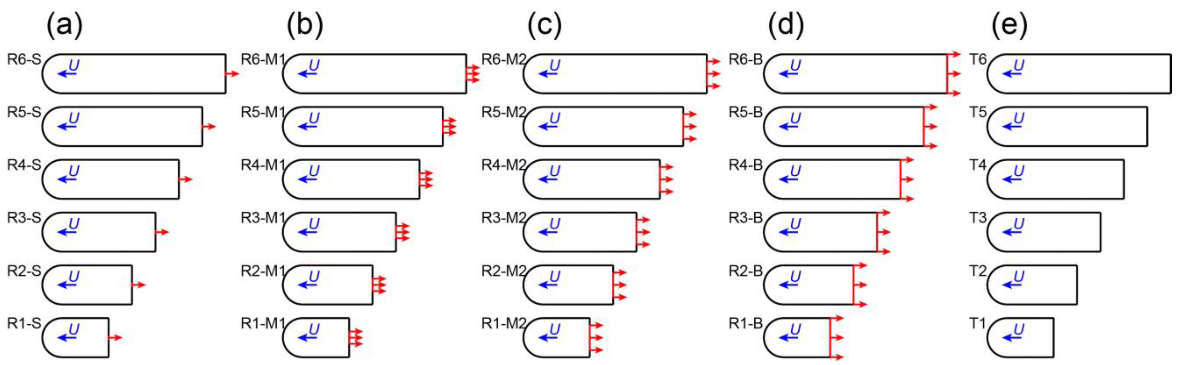
2.1. Body Geometry

In a highly idealized sense, four groups of self-propelled axisymmetric bodies are considered that swim steadily at a speed U via the rear-jetting single-jet propulsion but with four different jet orifice sizes (i.e., four different Ω values; Figure 1a–d). Each group consists of six bodies that have the same cross-sectional diameter d of 7.700 mm but different body aspect ratios (i.e., e ≡ (body cross-sectional diameter d)/(body length L) = 10/17, 10/23, 10/29, 10/35, 10/41, and 10/47, labeled, respectively, as R1-R6). Each body in the first group has a small jet orifice diameter d_orifice of 0.770 mm (i.e., Ω = 0.100; labeled as S; Figure 1a). Each body in the second group has a middle-sized d_orifice of 2.435 mm (i.e., Ω = 0.316; labeled as M1; Figure 1b). Each body in the third group has another middle-sized d_orifice of 4.870 mm (i.e., Ω = 0.632; labeled as M2; Figure 1c). Each body in the fourth group has the biggest d_orifice of 7.700 mm (i.e., Ω = 1.000; labeled as B; Figure 1d). An additional group consisting of six towed axisymmetric bodies is also considered that have the same d of 7.700 mm but different body aspect ratios (i.e., e = 10/17, 10/23, 10/29, 10/35, 10/41, and 10/47, labeled, respectively, as T1-T6; Figure 1e).

2.2. Computational Domain and Boundary Conditions

The present CFD study considers an axisymmetric body that moves steadily along its axisymmetry axis at intermediate Reynolds numbers (i.e., Re = U L/ν on the order of 1–1000, where ν is the fluid kinematic viscosity); thus, the flow around the body is assumed laminar, steady, and axisymmetric, and only a meridian plane is used as the computational domain to simulate such a flow. The axisymmetry axis of the body is taken as the axial x-axis and r being the radial distance from the x-axis, thereby forming a cylindrical polar coordinate system (Figure 2a).

The computational domain spans 50d in the x-direction and 25d in the r-direction. The discretization of the domain uses quadrilateral control volumes (CVs) with a constant mesh stretching rate of 1.04 applied to mesh points from the axisymmetric body to the domain boundaries (Figure 2a).

A symmetry boundary condition is prescribed on the upper boundary. A pressure-outlet boundary condition is prescribed on the right boundary. A stationary wall boundary condition is specified on the axisymmetric body, while the left boundary uses a velocity inlet boundary condition of a rightward velocity U to model the axisymmetric body swimming leftward at the speed U (Figure 2a). A velocity inlet boundary condition of a rightward velocity U_j is prescribed at the jet orifice to model the propulsive jet (Figure 2b).

2.3. Numerical Solver Specifications

The unstructured, finite-volume CFD software package ANSYS FLUENT (version 18.1.0) is used to numerically solve the steady incompressible Navier–Stokes equations and continuity equation, which govern the laminar, steady, and axisymmetric flow field around the steadily moving axisymmetric body, along with the above-described boundary conditions. The fluid density ρ is 1.0237 × 10³ kg m⁻³, and the fluid kinematic viscosity ν is 1.184 × 10⁻⁶ m² s⁻¹, both corresponding to seawater with salinity 32 at 15 °C at one normal atmosphere. The axisymmetric body is assumed to be neutrally buoyant.

The third-order Monotone Upstream-Centered Schemes for Conservation Laws (MUSCL) scheme is selected for spatial interpolation. The PREssure STaggering Option (PRESTO!) scheme is used as the pressure interpolation scheme. The Pressure-Implicit with Splitting of Operators (PISO) scheme is chosen for pressure–velocity coupling.

For a given jet-propelled body swimming steadily at a given speed U, a trial-and-error iteration method [32] is used to determine a jet velocity U_j such that the total jet thrust T equates the body drag D to at least seven significant digits, thereby numerically achieving self-propelled steady jet propulsion.

2.4. Performance Metrics

To illustrate the effects of jet orifice size on the performance of rear-jetting single-jet propulsion, drag coefficients, mechanical powers, swimming efficiencies, volume flow rates, and jet-propulsion performance indices are computed from the CFD-simulated flow fields.

The drag coefficient C_D is calculated as

$$C_{\mathrm{D}}\equiv \frac{D}{0.5\mathit{\rho }{U}^2{A}_{\mathrm{cs}}}=\frac{D_{\mathrm{viscous}}+D_{\mathrm{pressure}}}{0.5\mathit{\rho }{U}^2{A}_{\mathrm{cs}}}$$

(1)

where A_cs is the cross-sectional area of the axisymmetric body, D is body drag, D_viscous is viscous drag calculated as the axial component of the area integral of shear stress over the body surface, and D_pressure is pressure drag calculated as the axial component of the area integral of pressure over the body surface. Additionally, the viscous drag coefficient C_D-viscous is calculated as

$$C_{\mathrm{D}-\mathrm{viscous}}\equiv \frac{D_{\mathrm{viscous}}}{0.5\mathit{\rho }{U}^2{A}_{\mathrm{cs}}},$$

(2)

and the pressure drag coefficient C_D-pressure is calculated as

$$C_{\mathrm{D}-\mathrm{pressure}}\equiv \frac{D_{\mathrm{pressure}}}{0.5\mathit{\rho }{U}^2{A}_{\mathrm{cs}}}.$$

(3)

According to Ref. [1], the jet thrust T is calculated as

$$T=\mathit{\rho }{A}_{\mathrm{jet}}{U}_{\mathrm{j}}\left(U_{\mathrm{j}}-U\right),$$

(4)

where A_jet is the jet area. The jet power P_jet is calculated as

$$P_{\mathrm{jet}}=\frac{\mathit{\rho }{A}_{\mathrm{jet}}{U}_{\mathrm{j}}}{2}\left(U_{\mathrm{j}}{}^2-U^2\right).$$

(5)

According to Ref. [32], two well-defined swimming efficiencies can be calculated for jet propulsion, namely, the (conventional) Froude propulsion efficiency η_FPE and the quasi-propulsive efficiency η_QPE. They are, respectively, calculated as

$${\mathit{\eta }}_{\mathrm{FPE}}\equiv \frac{P_{\mathrm{useful}}}{P_{\mathrm{jet}}}$$

(6)

and

$${\mathit{\eta }}_{\mathrm{QPE}}\equiv \frac{P_{\mathrm{tow}}}{P_{\mathrm{jet}}},$$

(7)

where the useful power, P_useful = D U, is the mechanical power that is needed to overcome the resisting body drag acting on the body that swims steadily at the speed U via jet propulsion, and the tow power, P_tow = D_tow U, is the mechanical power that is needed to tow the same body, which is not jet propelled but towed, at the same speed U as in the jet propulsion, i.e., D_tow is the drag acting on the towed non-jetting body. The quasi-propulsive efficiency η_QPE is a rational non-dimensional metric of the propulsive fitness of a self-propulsion mechanism, which is used to compare mechanical power consumptions of different self-propulsion mechanisms under size and velocity constraints [33].

The jet volume flow rate Q is calculated as

$$Q=A_{\mathrm{jet}}{U}_{\mathrm{j}}.$$

(8)

A jet-propulsion performance index I_performance is defined as

$$I_{\mathrm{performance}}\equiv \frac{A_{\mathrm{cs}}U}{Q},$$

(9)

which is a non-dimensional metric of the effectiveness of jet propulsion, i.e., it compares swimming speeds sustained by differently sized jet orifices that eject the same volume flow rate.

2.5. Grid Refinement Study

The grid refinement study is performed for the jet-propelled body R6-M2 and the towed body T6 with three grids: (1) the baseline grid consisting of ~51,300 quadrilateral CVs, (2) the doubled grid consisting of ~161,200 quadrilateral CVs, and (3) the halved grid consisting of ~19,600 quadrilateral CVs. The results demonstrate excellent grid convergence between the baseline grid and the doubled grid (Figure 3). Therefore, the baseline grid is chosen for further simulations.

3. Results

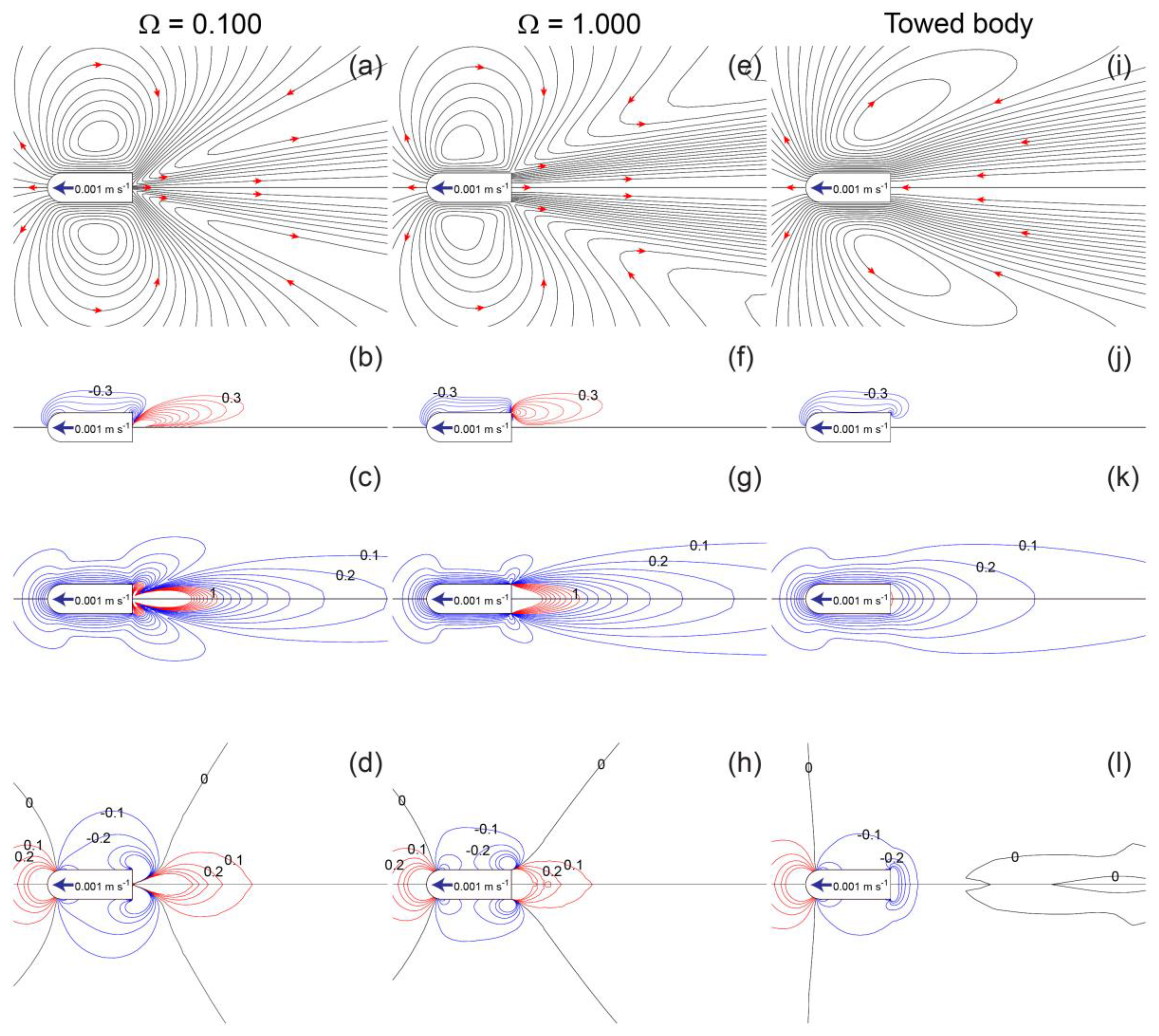
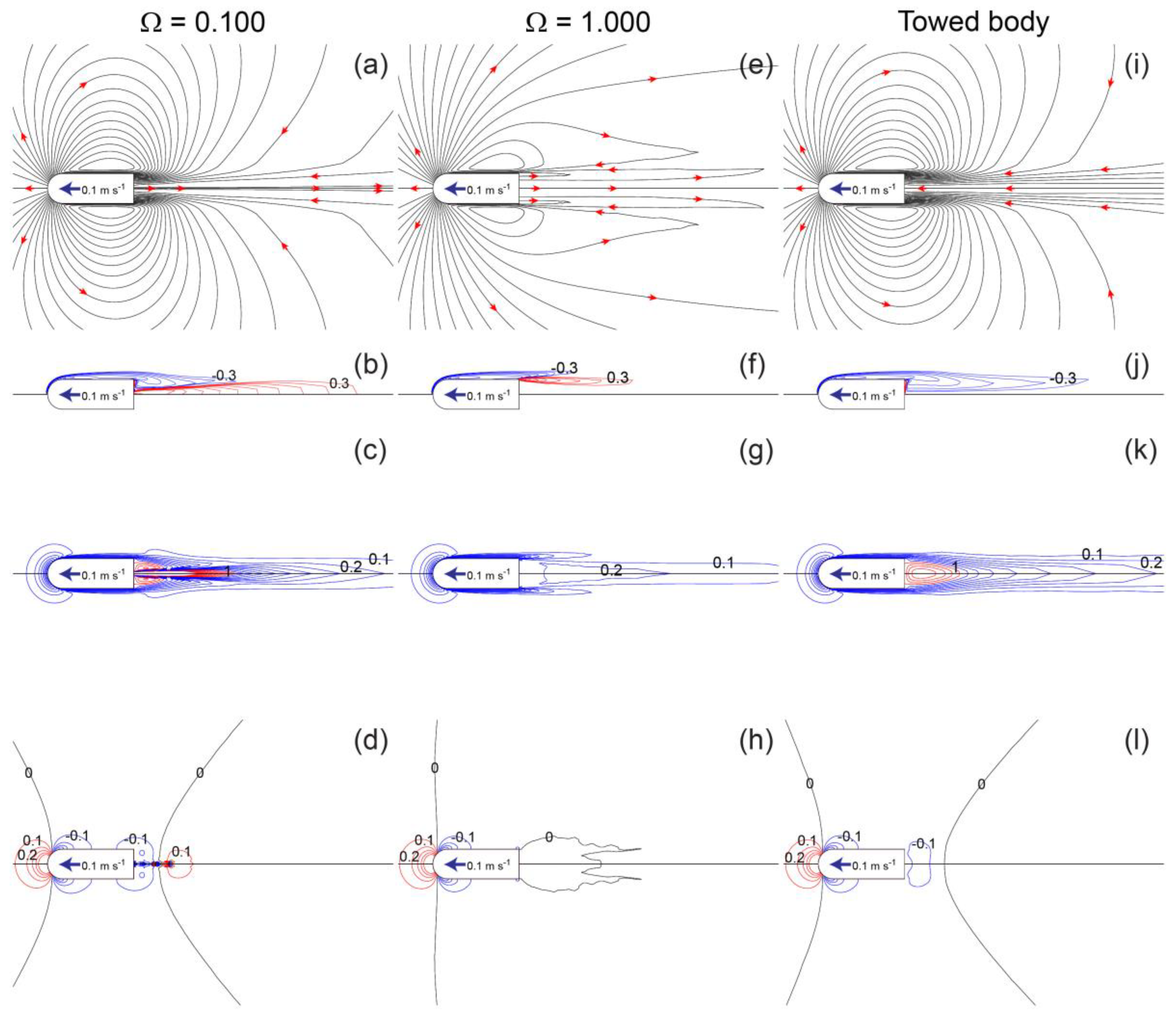
3.1. Simulated Flow Fields

For rear-jetting single-jet propulsion, the simulated flow fields vary with different Ω’s (orifice ratios) and Re’s. For example, comparing Ω = 0.1 and Ω = 1, at both Re = 18.9 (Figure 4) and Re = 1886 (Figure 5), the flow fields are almost identical around the front of the body but differ significantly behind the jet orifice: (1) the jet flow is narrower in Ω = 0.1 than Ω = 1; (2) the positive vorticity spreads further in the jet for Ω = 0.1 than Ω = 1; (3) the jet flow core extends further in Ω = 0.1 than Ω = 1; and (4) in Ω = 1 substantial overpressure develops at the entire rear end, especially at a low Re (Figure 4h), in contrast to in Ω = 0.1 where negative pressure dominates the rear-end region (Figure 4d and Figure 5d). Moreover, the flow field of a self-propelled jet propulsion body is completely different from that of the same body that is towed at the same speed (Figure 4 and Figure 5). For all situations, the flow velocity magnitudes decay spatially faster as Re increases (Figure 4c,g,k vs. Figure 5c,g,k).

3.2. Drag Coefficients

The drag force acting on a moving body depends on how the body moves through the fluid. The present CFD study shows that differences in drag coefficients arise between self-propelled jet-propulsion bodies and towed bodies, between self-propelled jet-propulsion bodies that have different Ω’s (orifice ratios), and between bodies that move at different Re’s (Figure 6). At the same Re and e (body aspect ratio), the self-propelled jet-propulsion bodies with Ω = 0.100, 0.316, and 0.632 all have a larger C_D-viscous (Figure 6b), C_D-pressure (Figure 6c), and C_D (Figure 6a) than the towed body. The self-propelled jet-propulsion body with Ω = 1.000 also has a (slightly) larger C_D-viscous than the towed body (Figure 6b); however, it has a smaller C_D-pressure than the towed body and even has negative C_D-pressure’s at lower Re’s (Figure 6c) because of the development of substantial overpressure at the entire rear end (Figure 4h). Therefore, the jet-propulsion body with Ω = 1.000 has a smaller C_D than the towed body (Figure 6a). Again, at the same Re and e, C_D-viscous increases only slightly as Ω increases from 0.100 to 1.000 (Figure 6b); however, C_D-pressure decreases substantially, especially at lower Re’s, as Ω increases from 0.100 to 1.000 (Figure 6c). As a result, C_D decreases as Ω increases from 0.100 to 1.000 (Figure 6a).

Drag coefficients that are obtained for bodies of all six body aspect ratios (e’s) are plotted in Supplementary Figure S1. For each e, the results follow similar patterns as above described. The whole dataset also shows that within a group of a given Ω or the towed body group, C_D decreases either as Re increases or as e increases (Supplementary Figure S1).

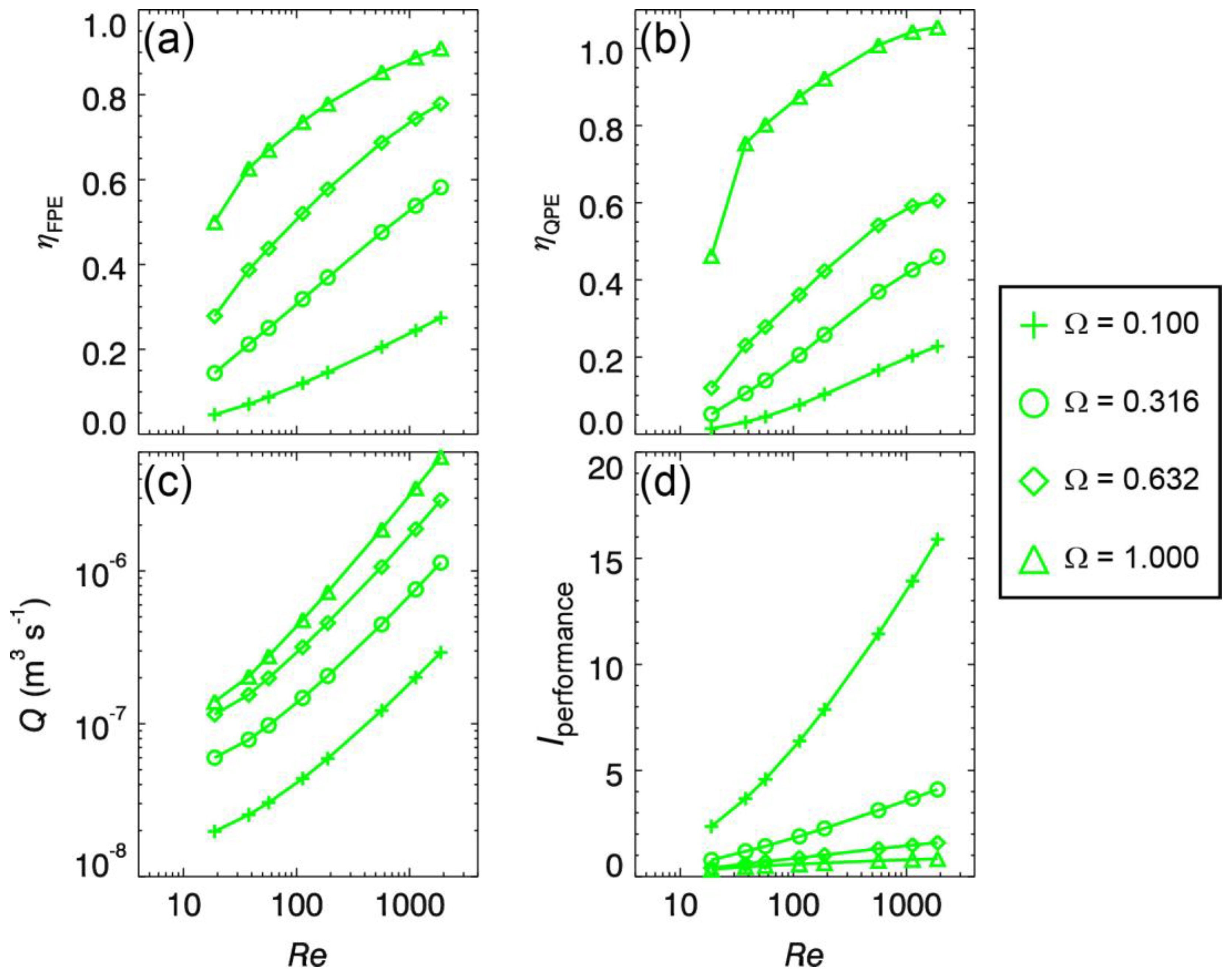
3.3. Swimming Efficiencies, Jet Volume Flow Rate, and Jet-Propulsion Performance Index

Froude propulsion efficiency (η_FPE), quasi-propulsive efficiency (η_QPE), jet volume flow rate (Q), and jet-propulsion performance index (I_performance) are impacted strongly by the orifice ratio Ω of the self-propelled jet-propulsion body. At the same Re and e (body aspect ratio), η_FPE (Figure 7a), η_QPE (Figure 7b), and Q (Figure 7c) all decrease as Ω decreases. In contrast, I_performance increases substantially as Ω decreases from 1.000 to 0.100 (Figure 7d). Thus, for a given Q, at the same e a jet-propulsion body with a smaller Ω sustains a considerably larger steady swimming speed U than that sustained by a jet-propulsion body with a larger Ω.

These performance metrics are obtained for self-propelled jet-propulsion bodies of all six body aspect ratios (e’s) and plotted in Supplementary Figures S2 and S3. For each e, the results follow similar patterns as above described. The whole dataset also shows that within a group of a given Ω, Q increases either as Re increases or as e decreases, while I_performance increases either as Re increases or as e increases (Supplementary Figure S3).

4. Discussion

The present CFD simulation study was directly motivated by the observational fact that most marine jet-propelled animals have low Froude propulsion efficiencies and small ratios of jet orifice diameter to body cross-sectional width (i.e., small Ω’s). Despite the highly complex biological reality of animal jet propulsion, the present study used a highly idealized CFD model that assumes steady axisymmetric flows for intermediate Re’s in the order of 1–1000. In doing so, the model was able to numerically achieve self-propelled steady swimming, i.e., the balance between total jet thrust and body drag, by using a trial-and-error iteration method. A comprehensive parametric study was also performed that systematically varies the orifice ratio Ω, the Reynolds number Re, and the body aspect ratio e, attempting to examine their first-order effects on animal jet propulsion.

The simulation results show that the swimming-imposed flow field, drag coefficients, swimming efficiencies, and jet-propulsion performance index all depend strongly on both the orifice ratio Ω and the Reynolds number Re and to a lesser degree on the body aspect ratio e (as shown by Supplementary Figures S1–S3). Most noticeably, both Froude propulsion efficiency and quasi-propulsive efficiency decrease considerably as the orifice ratio Ω decreases (i.e., as the jet orifice size decreases). On the contrary, the jet-propulsion performance index increases substantially as the orifice ratio Ω decreases (i.e., as the jet orifice size decreases), suggesting that, for a given jet volume flow rate, a smaller jet orifice can support faster swimming than a larger jet orifice can do, albeit at reduced swimming efficiencies. Equivalently, to swim at the same speed, a smaller jet orifice requires a lower jet volume flow rate than a larger jet orifice does. These results support the notion that most jet-propelled animals having relatively small jet orifice sizes may be an adaptation to deal with the physical constraint of limited total volume of water available for jetting, while needing to compete for a high swimming speed.

For self-propelled steady jet propulsion, the jet vorticity and the body vorticity are in balance, and their spatial distribution and mutual cancellation are strongly affected by the orifice ratio Ω. Irrespective of Re, the contact area between the negative body vorticity and the positive jet vorticity increases as Ω increases (Figure 4b,f and Figure 5b,f). As a result, as Ω increases, the negative body vorticity is more confined to the body and simultaneously the positive jet vorticity is less extended downstream, thereby decreasing the wake and increasing the Froude propulsion efficiency. This offers a simple explanation of increased swimming efficiency with increased Ω under the condition of self-propelled steady jet propulsion. Even in self-propelled, pulsed-jet propulsion that involves the unsteady interaction between jet-generated and body-shed vortices, it is suspected that the effects of jet orifice size on the evolution and cancellation of these vortices and therefore the wake characteristics should still be important; however, the detailed unsteady dynamics remains an unexplored research question.

As confirmed by the present investigation, there is a trade-off for jet-propelled animals whereby high thrust swimming achieved by having a small orifice ratio (Ω) greatly sacrifices swimming efficiency. While most jetting animals, such as squid and prolate medusae, use jet propulsion to achieve high swimming speeds and acceleration rates to evade predators or quickly reposition, some animals, such as salps, use jet propulsion for suspension feeding. It is found that the animals that use jet propulsion to escape predators and reposition have very small orifice ratios and, in fact, they have dynamic structures, such as velums, to further constrict their orifice during contraction phases of swimming which minimizes their orifice ratio. Efficiency is not as important for these types of swimmers.

However, jet-propelled animals that must swim continuously to feed must maximize efficiency. This is reflected in the large orifice ratios (Ω’s) observed among jet-propelled salps. For example, a salp Pegea confoederata was determined to have a maximum atrial siphon diameter of 1.23 cm and a body width of 2.84 cm, and a salp Cyclosalpa affinis to have a maximum atrial siphon diameter of 1.18 cm and a body width of 2.80 cm (both estimated from data presented in Figure 2 and

Table 1. List of symbols.

Symbol	Explanation
dorifice	Jet orifice diameter
d	Body cross-sectional width
L	Body length
Ω	Orifice ratio (≡ dorifice/d)
e	Body aspect ratio (≡ d/L)
α	Funnel ratio [≡ (maximum cross-sectional area of funnel)/(total volume)2/3]
U	Swimming speed
Uj	Jet velocity relative to the jet orifice
ν	Fluid kinematic viscosity
ρ	Fluid density
Re	Reynolds number (≡ U L/ν)
x	Axial coordinate
r	Radial coordinate
Dviscous	Viscous drag
Dpressure	Pressure drag
D	Body drag (≡ Dviscous + Dpressure)
Dtow	Drag acting on the towed non-jetting body
T	Total jet thrust
Acs	Body cross-sectional area (≡ π d2/4)
Ajet	Jet area (≡ π dorifice2/4)
CD-viscous	Viscous drag coefficient
CD-pressure	Pressure drag coefficient
CD	Drag coefficient (≡ CD-viscous + CD-pressure)
Pjet	Jet power
Puseful	Useful power (≡ D U)
Ptow	Tow power (≡ Dtow U)
ηFPE	Froude propulsion efficiency (≡ Puseful/Pjet)
ηQPE	Quasi-propulsive efficiency (≡ Ptow/Pjet)
Q	Jet volume flow rate
Iperformance	Jet-propulsion performance index (≡ Acs U/Q)

of Ref. [19]). Thus, salps have larger Ω’s (>0.42) than the other jet-propelled animals. Salps also differ in another aspect from those jet-propelled animals that use the same opening for jetting and refilling: Salps swim forward by drawing water in via the oral siphon and then expelling it through the atrial siphon, and they swim backward by switching the two siphons for drawing in and expelling water [17,18,19]. By using two siphons to respectively draw in and expel water, salps are less limited in the total volume of water available for jet propulsion, thereby having more room to use larger siphons to achieve higher swimming efficiencies. In fact, salps have been identified as the most efficient jet-propelled animal [17,18]. It is of great interest for future studies to investigate the fluid dynamics of salps that use two relatively large siphons to respectively draw in and expel water, in order to better understand salps’ unique way of propulsion and suspension-feeding mechanism.

References

1. Vogel, S. Life in Moving Fluids: The Physical Biology of Flow, 2nd ed.; Princeton University Press: Princeton, NJ, USA, 1994. [Google Scholar]
2. Alexander, R.M. Principles of Animal Locomotion; Princeton University Press: Princeton, NJ, USA, 2003. [Google Scholar]
3. Johnson, W.; Soden, P.D.; Trueman, E.R. A study in jet propulsion: An analysis of the motion of the squid, Loligo vulgaris. J. Exp. Biol. 1972, 56, 155–165. [Google Scholar] [CrossRef]
4. O’Dor, R.K. The forces acting on swimming squid. J. Exp. Biol. 1988, 137, 421–442. [Google Scholar] [CrossRef]
5. O’Dor, R.K.; Webber, D.M. Invertebrate athletes: Trade-offs between transport efficiency and power density in cephalopod evolution. J. Exp. Biol. 1991, 160, 93–112. [Google Scholar] [CrossRef]
6. Anderson, E.J.; DeMont, M.E. The mechanics of locomotion in the squid Loligo pealei: Locomotory function and unsteady hydrodynamics of the jet and intramantle pressure. J. Exp. Biol. 2000, 203, 2851–2863. [Google Scholar] [CrossRef] [PubMed]
7. Anderson, E.J.; Grosenbaugh, M.A. Jet flow in steadily swimming adult squid. J. Exp. Biol. 2005, 208, 1125–1146. [Google Scholar] [CrossRef] [PubMed] [Green Version]
8. Bartol, I.K.; Krueger, P.S.; Stewart, W.J.; Thompson, J.T. Hydrodynamics of pulsed jetting in juvenile and adult brief squid Lolliguncula brevis: Evidence of multiple jet ‘modes’ and their implications for propulsive efficiency. J. Exp. Biol. 2009, 212, 1889–1903. [Google Scholar] [CrossRef] [Green Version]
9. Packard, A.; Bone, Q.; Hignette, M. Breathing and swimming movements in a captive Nautilus. J. Mar. Biol. Ass. UK 1980, 60, 313–327. [Google Scholar] [CrossRef]
10. O’Dor, R.K.; Wells, J.; Wells, M.J. Speed, jet pressure and oxygen consumption relationships in free-swimming Nautilus. J. Exp. Biol. 1990, 154, 383–396. [Google Scholar] [CrossRef]
11. Neil, T.R.; Askew, G.N. Swimming mechanics and propulsive efficiency in the chambered Nautilus. R. Soc. Open Sci. 2018, 5, 170467. [Google Scholar] [CrossRef] [PubMed] [Green Version]
12. Daniel, T.L. Mechanics and energetics of medusan jet propulsion. Can. J. Zool. 1983, 61, 1406–1420. [Google Scholar] [CrossRef]
13. Colin, S.P.; Costello, J.H. Morphology, swimming performance and propulsive mode of six co-occurring hydromedusae. J. Exp. Biol. 2002, 205, 427–437. [Google Scholar] [CrossRef] [PubMed]
14. Dabiri, J.O.; Colin, S.P.; Costello, J.H.; Gharib, M. Flow patterns generated by oblate medusan jellyfish: Field measurements and laboratory analyses. J. Exp. Biol. 2005, 208, 1257–1265. [Google Scholar] [CrossRef] [PubMed] [Green Version]
15. Katija, K.; Jiang, H. Swimming by medusae Sarsia tubulosa in the viscous vortex ring limit. Limnol. Oceanogr. Fluids Environ. 2013, 3, 103–118. [Google Scholar] [CrossRef] [Green Version]
16. Katija, K.; Colin, S.P.; Costello, J.H.; Jiang, H. Ontogenetic propulsive transitions by Sarsia tubulosa medusae. J. Exp. Biol. 2015, 218, 2333–2343. [Google Scholar] [CrossRef] [PubMed] [Green Version]
17. Bone, Q.; Trueman, E.R. Jet propulsion in salps (Tunicata: Thaliacea). J. Zool. Lond. 1983, 201, 481–506. [Google Scholar] [CrossRef]
18. Madin, L.P. Aspects of jet propulsion in salps. Can. J. Zool. 1990, 68, 765–777. [Google Scholar] [CrossRef]
19. Sutherland, K.R.; Madin, L.P. Comparative jet wake structure and swimming performance of salps. J. Exp. Biol. 2010, 213, 2967–2975. [Google Scholar] [CrossRef] [Green Version]
20. Webber, D.M.; O’Dor, R.K. Monitoring the metabolic rate and activity of free-swimming squid with telemetered jet pressure. J. Exp. Biol. 1986, 126, 205–224. [Google Scholar] [CrossRef]
21. Jiang, H. An elastic collision model for impulsive jumping by small planktonic organisms. Fluids 2020, 5, 154. [Google Scholar] [CrossRef]
22. Dabiri, J.O.; Colin, S.P.; Katija, K.; Costello, J.H. A wake-based correlate of swimming performance and foraging behavior in seven co-occurring jellyfish species. J. Exp. Biol. 2010, 213, 1217–1225. [Google Scholar] [CrossRef] [Green Version]
23. Chamberlain, J.A.J. Jet propulsion of Nautilus: A surviving example of early Paleozoic cephalopod locomotor design. Can. J. Zool. 1990, 68, 806–814. [Google Scholar] [CrossRef]
24. Bartol, I.K.; Patterson, M.R.; Mann, R. Swimming mechanics and behavior of the shallow-water brief squid Lolliguncula brevis. J. Exp. Biol. 2001, 208, 1125–1146. [Google Scholar] [CrossRef]
25. Lighthill, M.J. Hydromechanics of aquatic animal propulsion. Annu. Rev. Fluid Mech. 1969, 1, 413–446. [Google Scholar] [CrossRef]
26. Jiang, H.; Grosenbaugh, M.A. Numerical simulation of vortex ring formation in the presence of background flow with implications for squid propulsion. Theor. Comput. Fluid Dyn. 2006, 20, 103–123. [Google Scholar] [CrossRef]
27. Bi, X.; Zhu, Q. Fluid-structure investigation of a squid-inspired swimmer. Phys. Fluids 2019, 31, 101901. [Google Scholar] [CrossRef]
28. Sahin, M.; Mohseni, K.; Colin, S.P. The numerical comparison of flow patterns and propulsive performances for the hydromedusae Sarsia tubulosa and Aequorea victoria. J. Exp. Biol. 2009, 212, 2656–2667. [Google Scholar] [CrossRef] [PubMed] [Green Version]
29. Herschlag, G.; Miller, L.A. Reynolds number limits for jet propulsion: A numerical study of simplified jellyfish. J. Theor. Biol. 2011, 285, 84–95. [Google Scholar] [CrossRef] [PubMed] [Green Version]
30. Hoover, A.P.; Griffith, B.E.; Miller, L.A. Quantifying performance in the medusan mechanospace with an actively swimming three-dimensional jellyfish model. J. Fluid Mech. 2017, 813, 1112–1155. [Google Scholar] [CrossRef]
31. Bi, X.; Zhu, Q. Dynamics of a squid-inspired swimmer in free swimming. Bioinspir. Biomim. 2020, 15, 016005. [Google Scholar] [CrossRef]
32. Jiang, H.; Costello, J.H.; Colin, S.P. Fluid dynamics and efficiency of colonial swimming via multijet propulsion at intermediate Reynolds numbers. Phys. Rev. Fluids 2021, 6, 013103. [Google Scholar] [CrossRef]
33. Maertens, A.P.; Triantafyllou, M.S.; Yue, D.K.P. Efficiency of fish propulsion. Bioinspir. Biomim. 2015, 10, 046013. [Google Scholar] [CrossRef] [PubMed] [Green Version]
Figure 1. (ad) Four groups of six jet-propelled axisymmetric bodies that have the same cross-sectional diameter but six different body aspect ratios combined with four different jet orifice sizes (i.e., four different Ω values). (e) A group of six towed axisymmetric bodies that have the same cross-sectional diameter but six different body aspect ratios. See the main text for detailed descriptions.
Fluids 06 00230 g001
Figure 2. Grid and boundary conditions for the axisymmetric CFD model: (a) the whole computational domain; (b) the near-body region. The grid shown here is for the jet-propelled body R3-M2, which consists of 36,154 quadrilateral control volumes (CVs).
Fluids 06 00230 g002
Figure 3. Results of grid refinement simulations of the jet-propelled body R6-M2 and the towed body T6: (a) velocity increment, UjU, in the jet, (b) drag coefficient CD, (c) quasi-propulsive efficiency ηQPE, and (d) Froude propulsion efficiency ηFPE, as functions of Re.
Fluids 06 00230 g003
Figure 4. Re = 18.9. CFD-simulated flow fields imposed, respectively, by the jet-propelled body R3-S (ad) and R3-B (eh) and by the towed body T3 (il), all of which move steadily at U = 0.001 m s−1. (a,e,i) Streamline patterns in a stationary frame of reference. (b,f,j) Contours of azimuthal vorticity scaled by 2U/d; red contour levels are 0.300, 0.443, 0.654, 0.965, 1.420, 2.100, 3.110, 4.590, 6.770, and 10.000; blue contour levels are −0.300, −0.443, −0.654, −0.965, −1.420, −2.100, −3.110, −4.590, −6.770, and −10.000. (c,g,k) Contours of velocity magnitude in a stationary frame of reference and scaled by U; red contour levels start from 1.0 with increment 0.1; blue contour levels start from 0.1 to 0.9 with increment 0.1. (d,h,l) Contours of pressure scaled by 0.5ρU2; red contour levels start from 0.1 with increment 0.1; blue contour levels start from −0.1 with increment −0.1; black contour lines are 0.
Fluids 06 00230 g004
Figure 5. Re = 1886.0. CFD-simulated flow fields imposed, respectively, by the jet-propelled body R3-S (ad) and R3-B (eh) and by the towed body T3 (i–l), all of which move steadily at U = 0.1 m s−1. Explanations of the panels are the same as in Figure 4.
Fluids 06 00230 g005
Figure 6. Line plots of (a) CD, (b) CD-viscous, (c) CD-pressure, and (d) CD-pressure/CD-viscous against Re, for the jet-propelled body R3-S (Ω = 0.100), R3-M1 (Ω = 0.316), R3-M2 (Ω = 0.632), and R3-B (Ω = 1.000), and for the towed body T3. All these bodies have the same body aspect ratio (i.e., e = 10/29).
Fluids 06 00230 g006
Figure 7. Line plots of (a) Froude propulsion efficiency ηFPE, (b) quasi-propulsive efficiency ηQPE, (c) jet volume flow rate Q, and (d) jet-propulsion performance index Iperformance against Re, for the jet-propelled body R3-S (Ω = 0.100), R3-M1 (Ω = 0.316), R3-M2 (Ω = 0.632), and R3-B (Ω = 1.000). All these bodies have the same body aspect ratio (i.e., e = 10/29).
Fluids 06 00230 g007