1. Introduction
This paper is part of the Special Issue honoring the contributions of W. W. Wilmarth to turbulence research. Bill Willmarth had a particular interest in turbulent boundary layers, especially the nature of the wall pressure fluctuations [
1] and the scaling of the Reynolds stresses [
2]. In addition, as noted by Blackwelder et al. [
3], he posed provocative questions regarding turbulent wall-layer structures, like “What are the effects of parameters, such as wall-roughness, pressure-gradients, surface-curvature, and three-dimensionality on the structure elements? How do the evolutionary histories of structures change with the above parameters?”
With regard to the behavior of canonical flows, especially flat plate boundary layers and fully developed pipe and channel flows, the last 10 to 20 years has seen an intense research effort that has brought great progress. Through a combination of pioneering experiments and computations covering a wide Reynolds number range, our knowledge of such flows has improved greatly. It is now well accepted that classical scaling laws combined with Townsend’s attached eddy hypothesis provide a fundamental framework for our present understanding. It has also become apparent that the effects of complexity can sometimes be included in this framework. For example, surface roughness can be incorporated simply as a change in the wall stress using Townsend’s hypothesis [
4], although the prediction of the wall stress as a function of the surface roughness is still a work in progress [
5]. In addition, under certain conditions the effects of pressure gradient can be included in this framework by using a model for the detached eddies [
6,
7].
These findings, however, have been mostly restricted to either fully-developed flows or boundary layers that exhibit self-similarity, that is, they scale according to local variables, such as the local freestream velocity , the friction velocity , and the boundary layer thickness . Here, , is the wall stress, and is the fluid density.
Another class of flows, of particular interest here, as it was to Willmarth, concerns the response to strong perturbations. For example, an equilibrium boundary layer may experience a sudden onset of wall curvature or flow divergence, or meet with an abrupt change in surface roughness [
8,
9,
10,
11]. Such flows were reviewed by Reference [
12] and have continued to draw interest since then [
13,
14,
15,
16,
17,
18,
19,
20,
21,
22,
23,
24,
25,
26,
27].
Almost all of these investigations consider only boundary layers, while the response of pipe flow to strong perturbations has received only limited attention. The response of pipe flow is different, primarily because of the geometric confinement associated with internal flows and the constraints on the flow response imposed by continuity. In some respects, however, pipe flows are an ideal place to explore the response of a wall-bounded flow to strong perturbations, from an experimental and numerical viewpoint, because the upstream and far-downstream conditions are well known, and very well defined at any Reynolds number. In addition, pipe flows are of enormous practical importance [
28], and in many applications experience a wide range of flow perturbations. Nonetheless, non-equilibrium pipe flows have not been explored to the same extent as their boundary layer counterparts, and the number of studies that have investigated the effects of strong perturbations on pipe flows is very small. Even if we include perturbed channel flows in the class of internal flows, the number does not grow much, and such studies are all relatively recent.
For example, Saito and Pullin [
29] performed a high Reynolds number large eddy simulation (LES) study of turbulent flow in a long channel that experienced repeated transitions between smooth and rough surfaces. For a given transition, they found that the friction velocity first overshot and then undershot their equivalent equilibrium value before finally recovering over a stream-wise distance of order 10–30
h, where
h is the channel half-height, depending on both roughness and Reynolds number. These observations are in line with the response of boundary layers to a change in surface roughness [
30,
31], but they noted the important role played by confinement due to the channel geometry. They used the example of a smooth-to-rough transition to illustrate this phenomenon. The velocity abruptly experiences a deficit near the wall as it first encounters the increase in surface roughness. To maintain continuity, this constitutes a loss of stream-wise mass flux near the wall that requires an equal increase of stream-wise mass flux farther away from the wall. Since the boundary layer has a semi-infinite vertical extent, such an increase in flux away from the wall is noted only as a slight increase in velocity. In a steady channel flow, however, velocity increases in the outer region are expected to be correspondingly more significant. This was indeed the case.
More recently, Ismail et al. [
32,
33,
34] reported direct numerical simulations (DNS) of channel flow undergoing a step change from either a rib- or cube-roughened surface to a smooth wall. They estimated that the recovery distance in the outer flow was on the order of 50 channel half-heights, and different statistics were adjusting at dissimilar rates. Notably, the expansion of the flow after the step change produces strong advection effects and an adverse pressure gradient, which delay the emergence of the logarithmic law to an estimated distance of about
–20. The dominant momentum balance in the developing regime was between strong advection and turbulence fluxes.
Here, we discuss some recent experimental results that expand our understanding of strongly perturbed pipe flows [
35,
36,
37,
38,
39,
40]. Three cases are considered: the recovery from a step change in roughness from rough to smooth; the relaxation downstream of a single square bar roughness element of different heights; and the recovery of the wake downstream of a body-of-revolution placed on the centerline of the pipe. This summary of recent work is more in the service of assessing our present knowledge of perturbed pipe flows, rather than an original research contribution, and so we are particularly interested in drawing out the similarities observed in the more general flow response. We will see that this class of perturbed flows, especially their characteristically slow relaxation behavior, can be connected to a second-order flow model derived from the RANS equations. We begin by presenting brief summaries of the data for all three experiments, and then discuss the modeling effort and how it can be used to unify the observational experience.
2. Flow Past a Step-Change in Wall Roughness
Van Buren et al. [
37] studied the propagation of disturbances in pipe flow following a rough-to-smooth step change in wall condition. The pipe radius
R was 19.1 mm with a bulk velocity of 3.45 m/s. This resulted in a diameter-based Reynolds number of
. The flow developed over sand-grain roughness, with an equivalent roughness of
µm, for a distance of 100 diameters before the surface abruptly changed to a smooth wall. The flow downstream of the step change was measured in cross-sectional planes—at
, 6.4, 9.2, 13.4, 19.4, 28.4., 41.2, 60, 80, 100, and 120, where
is measured from the start of the smooth pipe—using stereoscopic particle image velocimetry (SPIV), which gives all three components of velocity on a two-dimensional plane. Pressure measurements were also made at multiple locations downstream of the step using a freestanding manometer.
In a fully-developed pipe flow, the area- and time-averaged pressure gradient
balances the wall shear
exactly, but, when the flow is in a state of development, the stream-wise gradient of the momentum flux
also contributes to the force balance. The notation is such that
is the mean stream-wise velocity and
is the fluctuating stream-wise velocity.
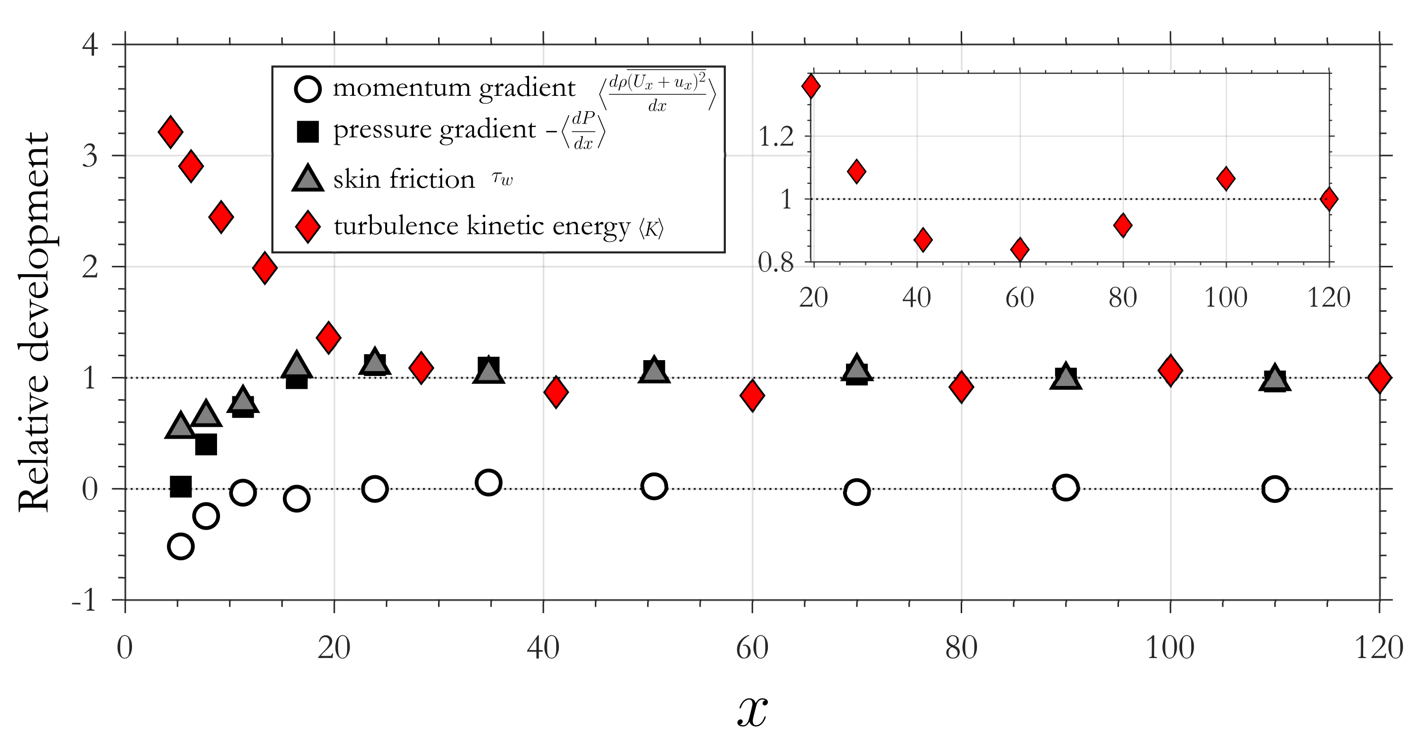
Figure 1 shows the various contributions made by the momentum gradient, pressure gradient, and wall shear in the experiment as the flow responds to the step change. The development of the area-averaged turbulence kinetic energy
is also shown. This figure displays
relative development, where the pressure gradient, skin friction, and turbulence kinetic energy are normalized by their values at the farthest downstream location, which was taken as an estimate of the fully relaxed state. For a short region downstream of the step change, the wall shear, momentum gradient, and pressure gradient are all lower than in the fully-developed smooth-wall case. These quantities recover relatively quickly, however, and, by
, they have approximately reached their fully-developed values. The turbulence kinetic energy level, however, displays small oscillations that persist much farther downstream. This oscillatory response of the flow statistics and its asymptotically slow relaxation, shown here by the turbulence kinetic energy, are unifying features of the three flows considered in this paper.
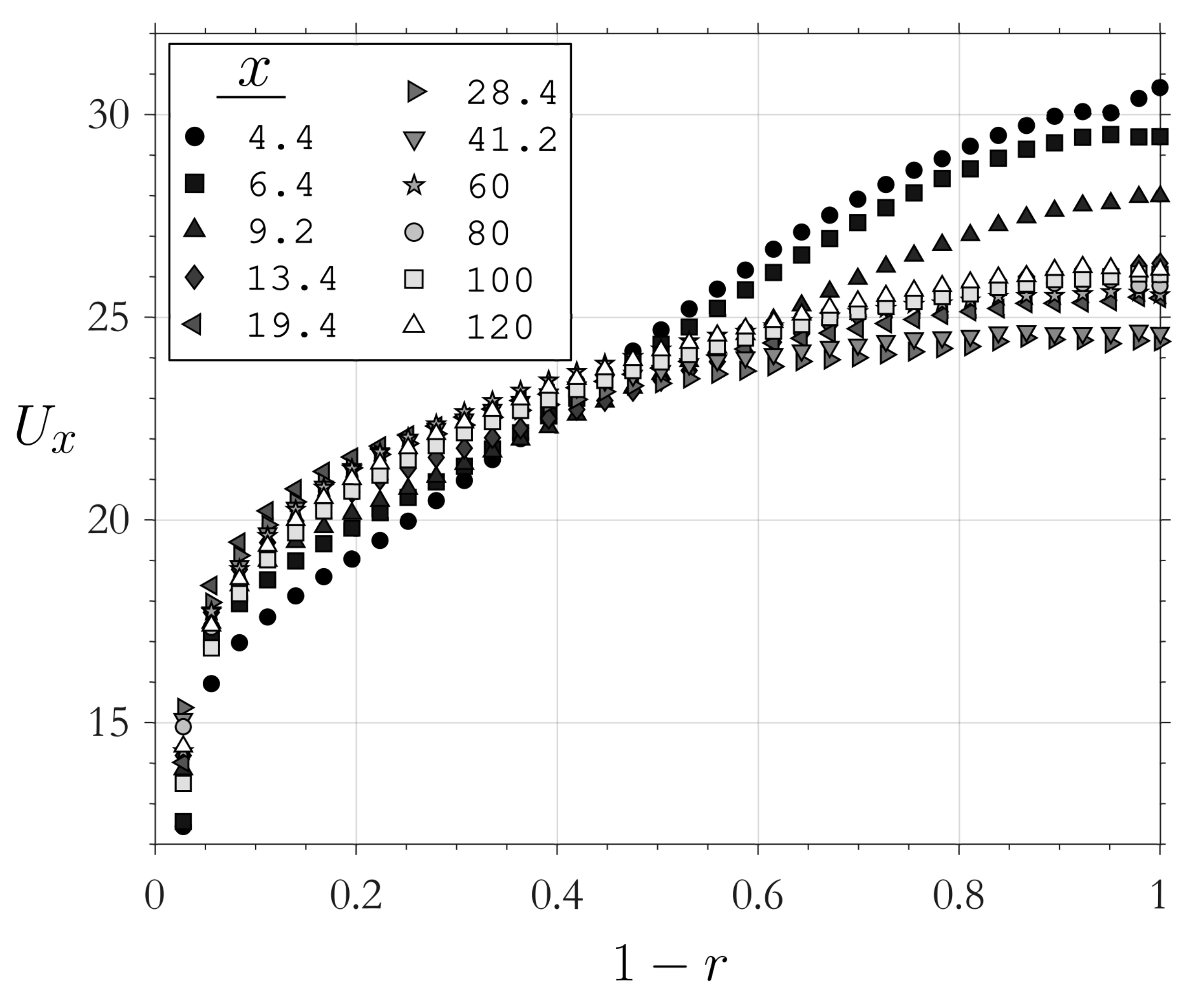
As the flow moves from the rough pipe into the smooth one, the shear at the wall changes abruptly, and the subsequent acceleration at the wall must be balanced with a deceleration in the pipe center because of continuity. This can be most clearly seen via the downstream development of the mean stream-wise velocity profiles shown in
Figure 2. The radial coordinate is
; we will also use the wall distance
. Note that all quantities are given non-dimensionally, normalized using the pipe radius
R and
, the friction velocity value expected to occur very far downstream of the step change.
The flow can be analyzed using the Reynolds Averaged Navier–Stokes equations (RANS) for the stream-wise component (bearing in mind that we are considering a non-equilibrium flow)
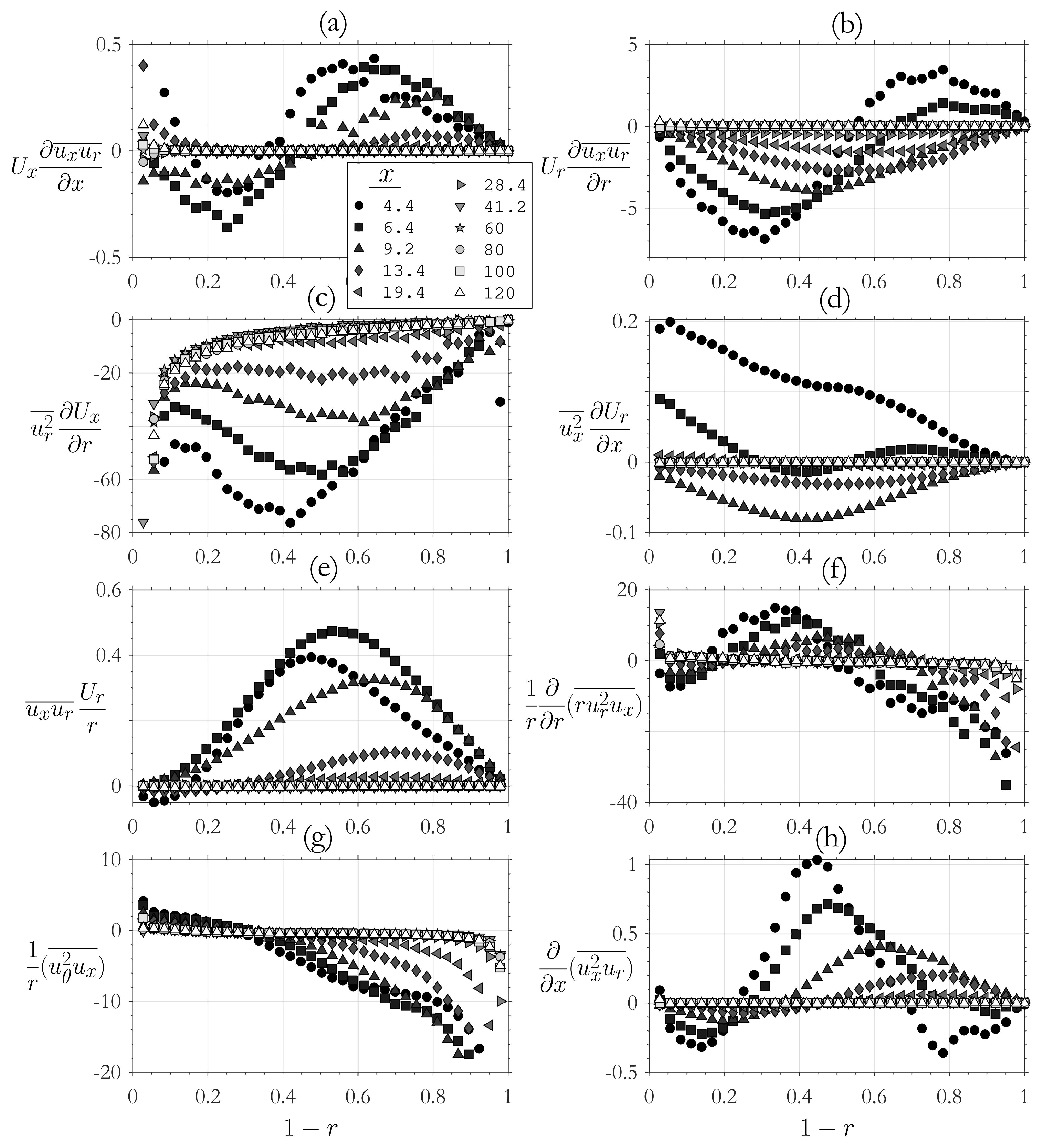
The dominant acceleration is , and the data indicated it was balanced primarily by the wall-normal gradient of the Reynolds shear stress, . It is, therefore, useful to examine the Reynolds stress transport equation, which can be written as a balance of production, turbulent diffusion, pressure diffusion, pressure strain, viscous diffusion, and viscous dissipation.
According to the data shown in
Figure 3, the turbulent diffusion terms are important very close to the step, but they quickly become negligible with distance downstream. Far downstream, the Reynolds stresses evolve through a simple balance between one of the production terms,
, and the pressure strain term. The production acts as a source of the Reynolds stress
, and the pressure strain term works against anisotropy in the turbulence energy and is, thus, a sink of
. This observation is crucial to the development of the far-field recovery flow model given in
Section 5.
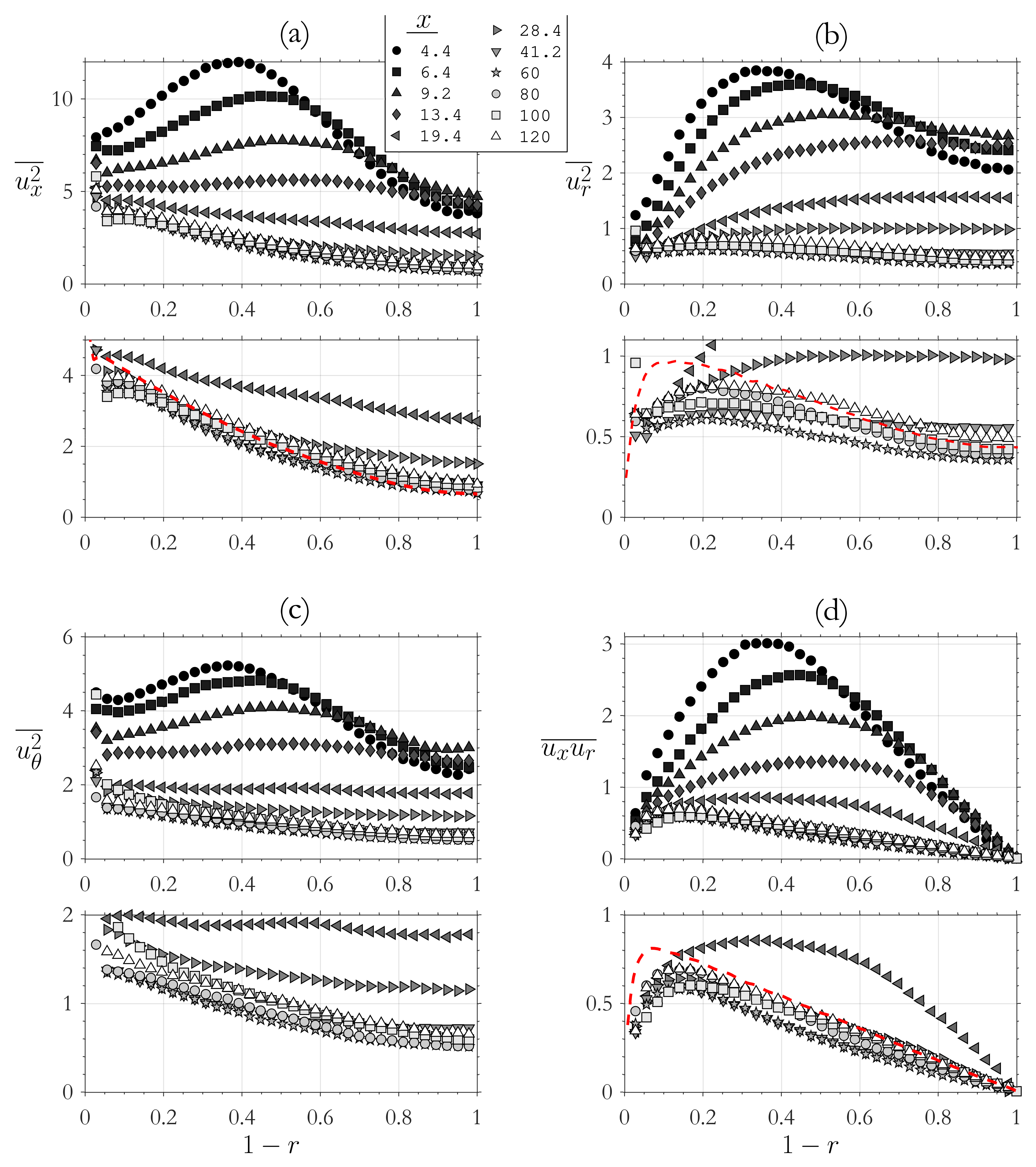
Profiles of the different sources of turbulence kinetic energy:
,
,
, and
, are presented for this experiment in
Figure 4. These profiles indicated that, while some terms were larger than others, they all responded in a broadly similar to the change in wall condition. That is, for all the stresses, the peak of the disturbance is in the same radial location, the relative size of the peak is consistent, and the shape of the disturbance is approximately parabolic away from the centerline (these aspects were discussed in more detail by Reference [
37]). In the simple model of the flow described in
Section 5, therefore, it will be assumed that the disturbance takes the same shape for all fluctuation components.
A particularly important finding is that the disturbances are evident very far downstream, exceeding the 120 pipe radii measurement domain. Additionally, the response was oscillatory, overshooting the eventual fully-developed condition in a second-order response.
To assess the influence of flow structures on the statistical response, Fourier decomposition and proper orthogonal decomposition may be applied in the azimuthal and radial directions, respectively. As has been found in the past [
41,
42], this approach can be used to identify large-scale motions in pipe turbulence. Van Buren et al. [
37] found that the larger structures were the slowest to respond to the step-change in wall roughness, as is to be expected, and that they were primarily responsible for the second-order like response, which may not be as expected.
3. Flow Downstream of a Square Bar Roughness Element
The next case we consider is the relaxation of turbulent pipe flow downstream of a square bar roughness element [
38,
40]. The experiment was conducted in the same recirculating pipe facility used by Van Buren et al. [
37], and the perturbation was introduced axisymmetrically by mounting a square-cross-section ring on the pipe wall at about 100
D downstream of the entrance to the pipe. Three bar heights,
0.04, 0.1 and 0.2, were employed to vary the perturbation strength. The upstream flow was fully developed at a bulk Reynolds number
, corresponding to a friction Reynolds number
. (The Reynolds number dependence of the flow for
0.1 was recently examined using RANS modeling by Reference [
43]). PIV measurements were performed in the axial-radial plane at distances up to
(
x is measured from the downstream side of the square bar).
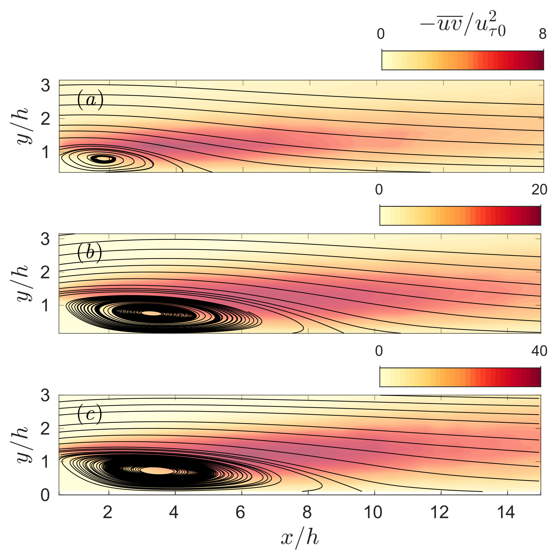
The mean streamlines in the region close to the separation bubble are shown in
Figure 5, together with the corresponding shear stress distributions. For all three bars, the flow is seen to separate at the leading edge of the bar, and then the mean dividing streamline rises a little above the location where
before bending down toward the reattachment point. At the same time, the peak in shear stress moves slowly away from the wall.
Ding and Smits [
40] found that the recovery of the flow is characterized by different scaling laws and transport mechanisms in the near field and the far field, with their stream-wise extents determined by
. In the near field (
), the flow in the central region of the pipe first accelerates to maintain continuity and then gradually slows down, as shown in
Figure 6a. The mean velocity profiles relax by pivoting: far from the wall the flow decelerates, while, near the wall, it speeds up. The mean momentum budget indicates that in the near field the near-wall acceleration is primarily attributed to momentum flux towards the wall, whereas the retardation in the central region is driven by adverse pressure gradients. It was also found that the mean pressure gradient recovers to its equilibrium value at about
, corresponding to
,
, and
for the small, medium, and large bars, respectively. In the far field, shown in
Figure 6b, the mean flow relaxation slows down, but, by
, it has almost fully recovered.
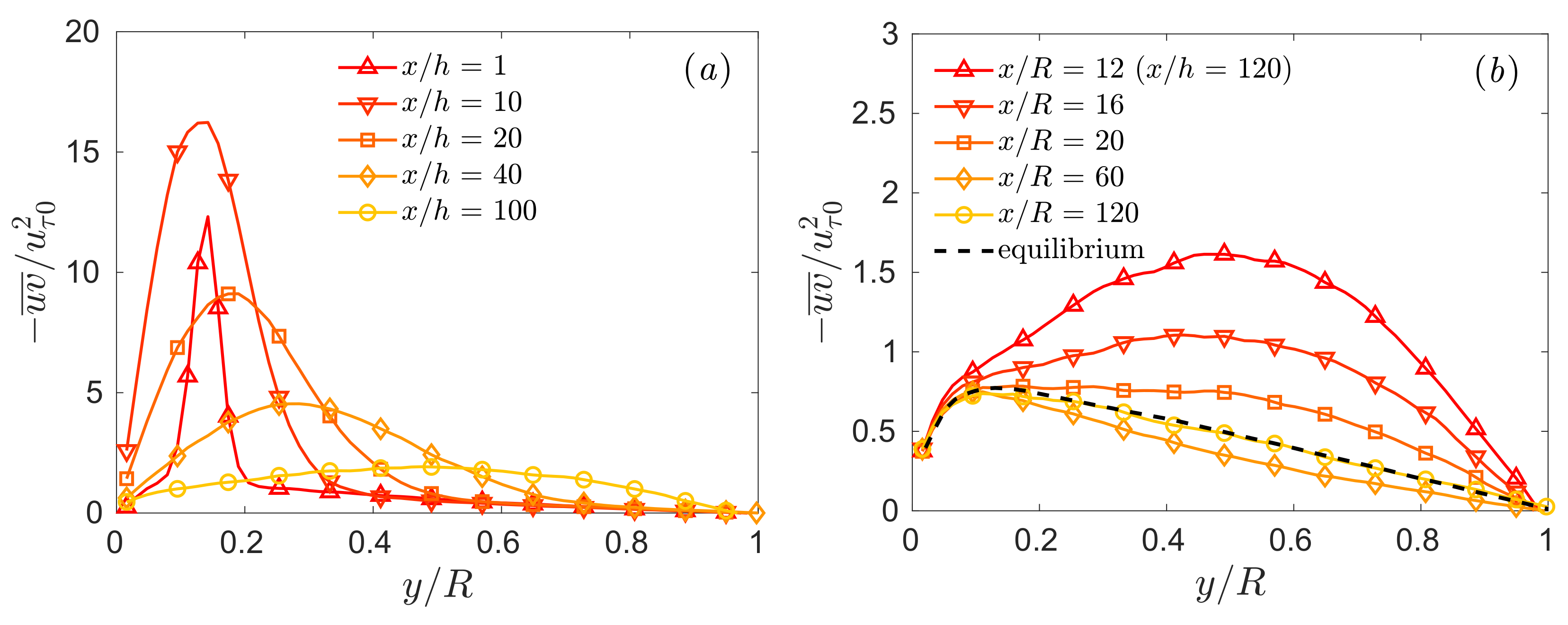
The development of turbulent shear stress in the near field is presented in
Figure 7a for the case where
. It is seen that the shear layer produced by the square bar is initially confined in a region close to
(that is,
) before it starts to diffuse outwards. The diffusion or redistribution of turbulence is a result of turbulent convection in the wall-normal direction (i.e., the triple correlation term
in the transport equation for
). In the far field, shown in
Figure 7b, the shear stress distribution for
maintains an approximately similar shape as it decays, but it eventually falls below the equilibrium levels before recovering to its expected distribution by
.
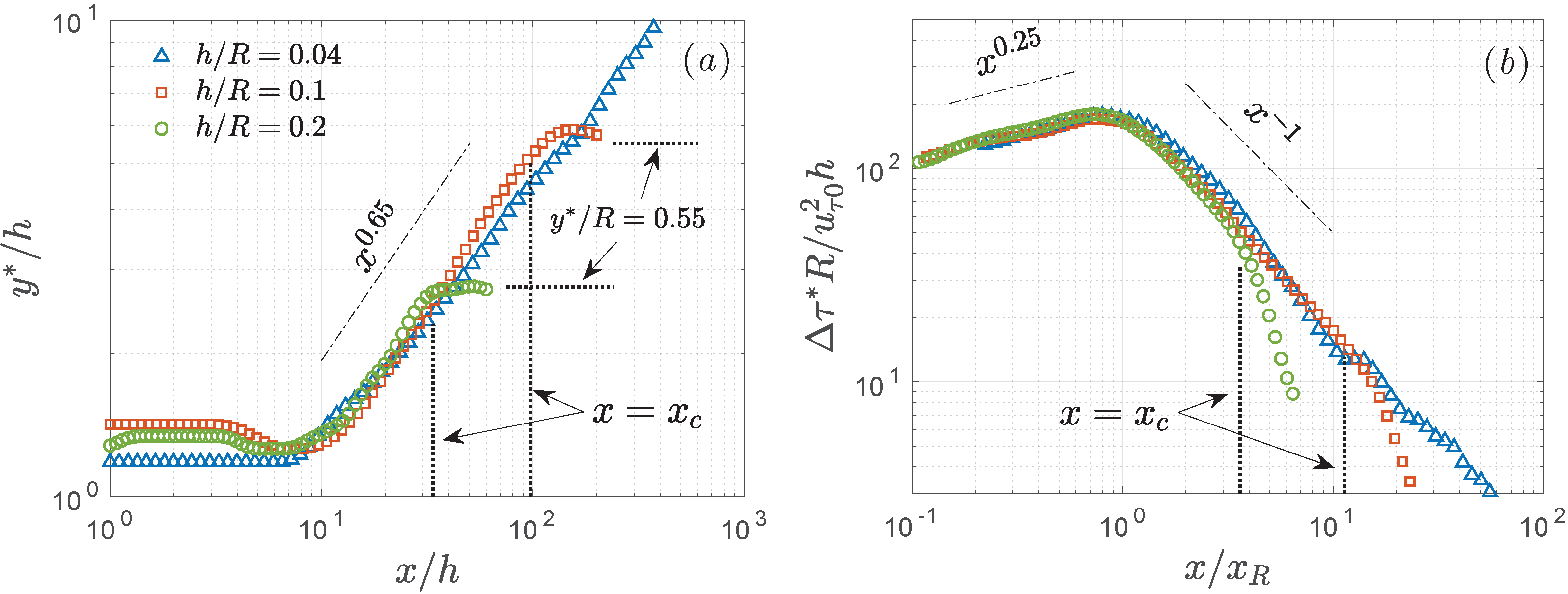
The scaling of the response is represented by the development of
and
as a function of
, as shown in
Figure 8. Here,
is the maximum excess shear stress with respect to the fully developed state in a given profile, and
denotes the wall-normal location of
.
Figure 8a shows that downstream of
,
moves towards the pipe centerline as a result of turbulent convection, and it closely follows a power law
. The power law variation holds up to the point where
, which marks the end of the region where turbulent convection is important. This point corresponds to a stream-wise distance
, which Ding and Smits [
40] called the convection length scale.
As to
, its amplitude scales with
, as is seen in
Figure 8b for both the growth and the decay region. The maximum
occurs at approximately the reattachment distance
, and it then decays approximately as
up until the point where
.
We see that the redistribution of turbulence, in which the turbulent convection
plays a central role, is a defining mechanism in the initial response of the flow. During the redistribution process,
is negative near the wall and positive away from the wall, thus moving
towards the centerline (i.e.,
increases with
x), as seen in
Figure 7a. Given the axisymmetry of a pipe,
is zero at both
and
, so that the increase of
ceases when
exhibits a more or less symmetric shape over
. The location where
stops increasing is
, and it also marks the location where
peels off from the −1 power law decay. It is worth emphasizing that
scales inversely with
, that is, the convection process lasts longer for a smaller bar. However, when
becomes sufficiently small, the magnitude of
decreases to almost zero before
, as was observed for the small bar case (
). For the larger bars,
= 100 and 33 (
= 10 and 6.7) for
= 0.1 and 0.2, respectively.
For the far-field development (
), a few distinct features are observed in
Figure 6b and
Figure 7b. First, we see that the
profile maintains a roughly similar shape, while its peak value slowly decays, initially undershooting the equilibrium profile before finally reaching the equilibrium values by
. Second, the recovery is long-lasting with a stream-wise extent on the order of
, whereas the reattachment and convection occur within the initial
. In addition, both the mean flow and the turbulent shear stress exhibit an oscillatory recovery behavior. This is more obvious for the shear stress, which falls below the equilibrium profile before rising up again (
Figure 7b).
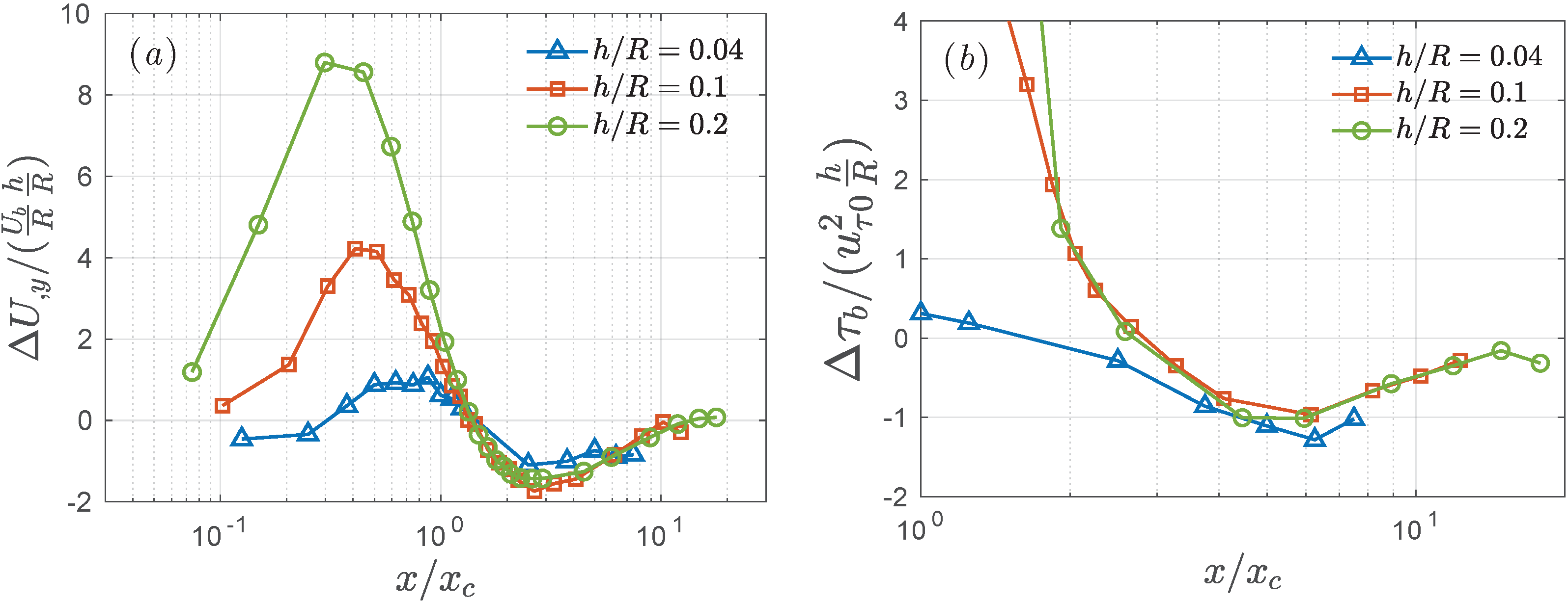
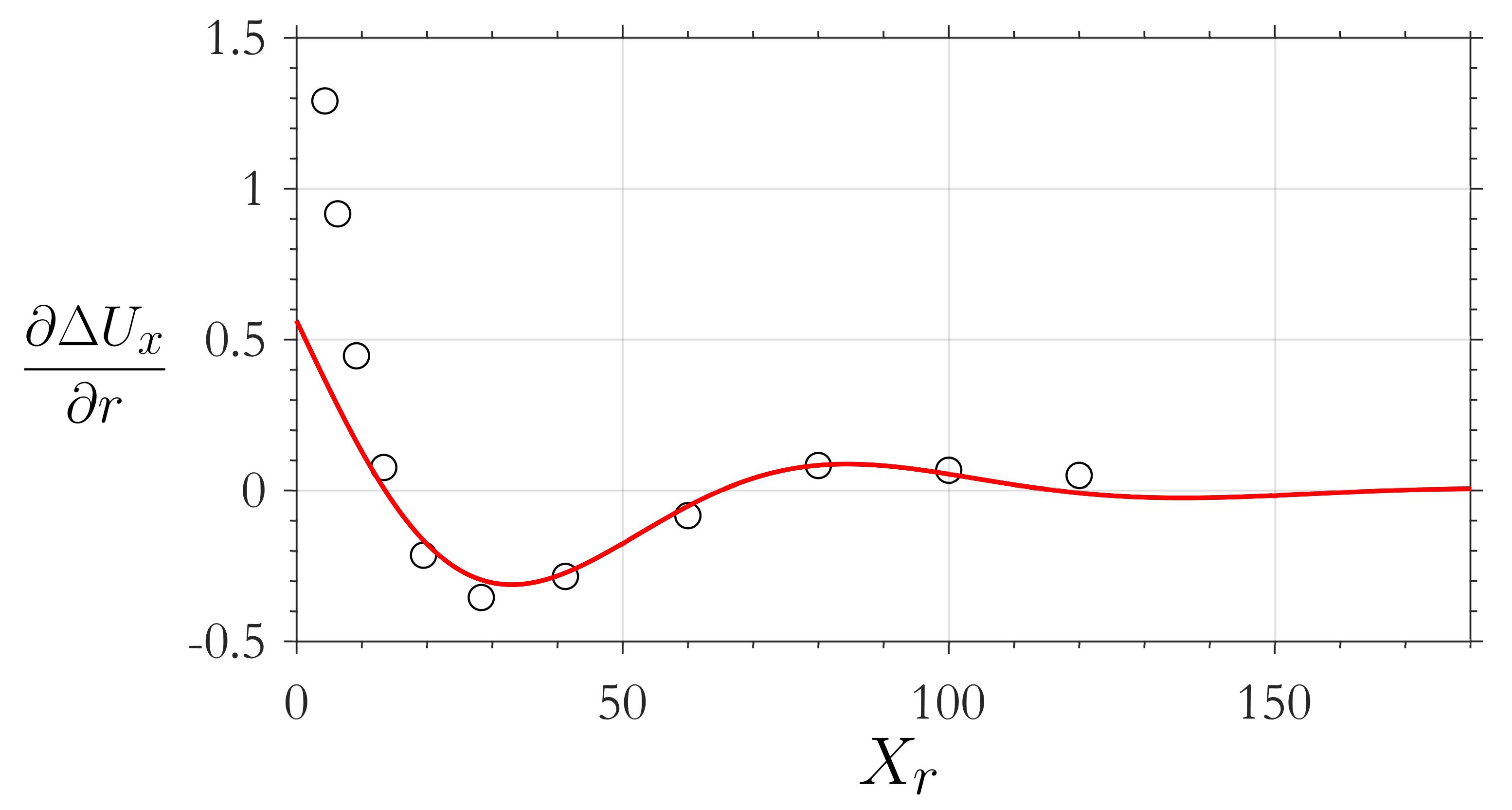
Figure 9 presents the far-downstream development of the disturbance
. Here,
is the maximum excess mean velocity gradient
with respect to the fully developed state in a given profile, and similarly for
where
is the bulk (integrated) shear stress. Both
and
display similarity in their stream-wise development when viewed against
, and
lags behind
by
, that is, where
crosses zero corresponds to the maximum
. The oscillation half-wavelength, as measured by the distance between the two zeros-crossings, is approximately 12.5
for both
and
. The similarity scale for the amplitudes of
and
was found to be simply
, as seen from the collapse of data in
Figure 9. The picture of the far-field recovery then becomes clear—as the perturbation strength (as measured by
) increases, the mean flow statistics oscillate with a smaller wavelength (
in terms of
R) and a larger amplitude (
). In addition, the oscillatory behavior is almost the same for the mean flow and the turbulence, except for a
phase difference. The above findings have made it clear that the scales governing the flow development transition from
h and
in the near field to
in the far field.
It was discussed in Reference [
40] that the far-downstream recovery is driven by the interaction between the mean flow and the turbulent shear stress, and the oscillatory behavior results from the asynchronous recovery between the two quantities. The oscillation amplitude decays for both quantities, and the final recovery is achieved when the oscillation amplitude becomes sufficiently small. The damped oscillatory recovery has its roots in the transport equations and is a common behavior for relaxing wall-bounded flows [
9,
32,
37].
4. Flow Downstream of a Streamlined Body of Revolution
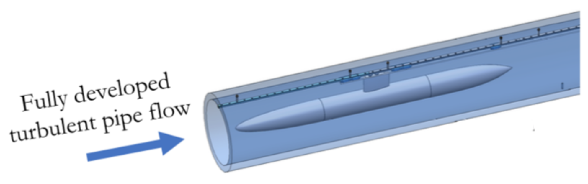
Both the step roughness change and the single square bar roughness element are perturbations in wall conditions. Here, we discuss a different test case where the pipe flow is perturbed by a streamlined body of revolution placed symmetrically on the centerline, as shown in
Figure 10. As in the other cases, the upstream unperturbed flow was fully developed with a bulk Reynolds number of 165,000. The body consisted of three sections—a prolate spheroidal bow section, a cylindrical mid-body region, and a stern section with a sharp tail designed to avoid separation. The body affects the flow in a complex manner involving spatially-developing pressure gradients and streamline curvature and divergence/convergence. Three body diameters were investigated, with blockage ratios of 1/9, 2/9, and 1/3. Planar PIV data were collected in the axial-radial plane over the entire body length, as well as in the near and far wakes. Here, we focus on the flow relaxation in the wake of the body with a blockage ratio of 1/3. Further detail of the body geometry, as well as the flow development in the bow and mid-body regions, can be found in Reference [
44].
The mean momentum budget indicates that immediately downstream of the body the mean flow development is driven by both the pressure gradient () and the turbulent shear stress (). The mean pressure gradient then recovers quickly in a few radii so that, farther downstream, the variation of U is primarily due to momentum flux. The evolution of momentum flux, as characterized by , is governed by the interaction between the mean flow and Reynolds stress, which is a slow and oscillatory process, similar to the relaxation downstream of the step roughness change and the square bar roughness element.
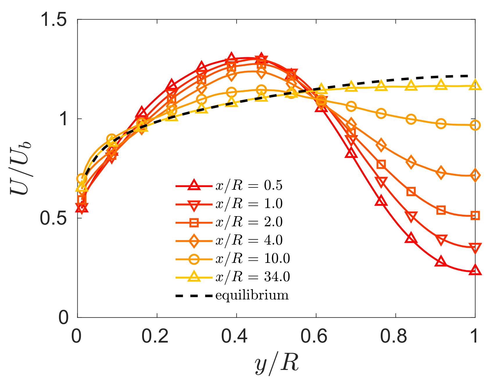
Figure 11 presents the evolution of the mean axial velocity in the wake, where
x is measured from the stern,
y is the wall-normal coordinate, and
R is the pipe radius. The mean velocity distribution in the wake can be viewed in terms of three regions—a layer near the pipe wall, a velocity defect region in the central part of the flow (the true wake, approximately defined by
in this example), and a high-speed region centered at about
that forms as a result of the flow acceleration due to blockage. The velocity in the wake undergoes an initial rapid recovery followed by a much slow development farther downstream. As shown in the figure, the velocity at the centerline accelerates from 15% to 80% of
over the initial 10 radii (where
is the equilibrium centerline velocity), and then increases slowly to about
by
. To maintain continuity, the acceleration near the centerline is accompanied by the deceleration seen for
, forming a pivot point near
. This pivoting behavior was also observed in the relaxation downstream of the square bar perturbation (see above) and is associated with momentum transfer by turbulent mixing [
40]. As to the near-wall layer, it speeds up exiting the stern region, and it develops an overshoot above the fully-developed profile at
. Farther downstream at
, the mean velocity distribution over
nearly coincides with the equilibrium profile, except for a slight defect near the centerline.
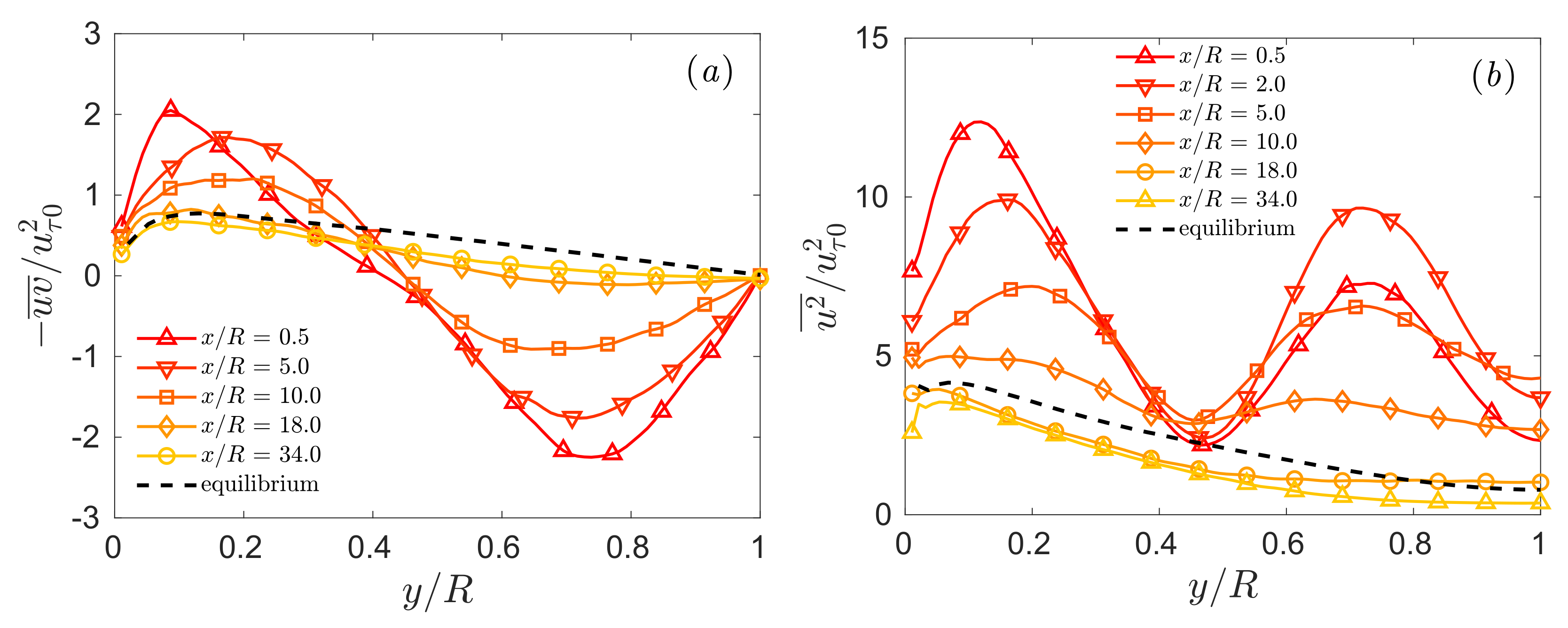
The relaxation of turbulent shear stress is shown in
Figure 12a. Intense turbulent mixing is seen near both the pipe wall and the centerline. Near the pipe wall, the peak of
occurs at
immediately downstream of the body and then moves to
followed by a decay towards the equilibrium profile. This redistribution and decay process for the turbulent shear stress was also observed in the earlier examples for the step change in roughness and the square bar element where the perturbation produces excess turbulence near the wall [
37,
40]. Away from the wall in the region of negative velocity gradient (
),
changes sign, implying a mean momentum exchange in the opposite direction. The overall relaxation of
occurs at a high rate initially and then drastically slows down as it approaches the equilibrium profile, much like that observed in other perturbed wall turbulence flows. The redistribution and decay is also observed for the evolution of
in
Figure 12b. The second-order response is again evident—an undershoot below the equilibrium profile is seen at
= 18 and 34. The fact that the distribution of
changes very little over
suggests that the second-order response has a rather long wavelength and the recovery overall is long-lasting, a behavior that is again displayed by the step roughness change and the single square bar roughness element. Additional measureemtns farther downstream will be needed to investigate this behavior more fully.
5. Modeling Non-Equilibrium Wall-Bounded Turbulence
For all three examples discussed here, for the region beyond where turbulent convection/diffusion is important, we have a balance between production and pressure strain. In addition, in this region the disturbance profile (the measure of how far the stresses are away from their equilibrium values) maintains an approximately similar shape with distance downstream, and it can be characterized by a single variable, its peak height. This leads us to consider a model for the far-field recovery in terms of the RANS equations, particularly the shear stress transport equation.
Non-equilibrium turbulence has been successfully modeled in the past, with limitations. Both References [
9,
37] developed a model for perturbed wall-bounded turbulence where the shape of the disturbance is assumed. The models describe the outer flow response where the large-scale motions with long time scales are key to understanding the long-lasting second-order response. Below is a summary of this modeling strategy, most recently used by References [
37,
40].
The model is based on two equations. First, the stream-wise RANS equation, differentiated by the wall-normal coordinate
r and re-organized using continuity,
Note here that
. Stream-wise gradients outside of the material derivative are neglected because the flow development itself is governed by wall-normal gradients. The second equation is the transport of
:
where it is assumed that the turbulent and pressure diffusion in the outer layer are negligible (supported by Reference [
45]). Therefore, the transport of
is governed by the competing contributions from production and pressure strain. The pressure strain terms are then broken into the “slow” and “fast” components [
46] and then modeled following References [
47,
48].
These two main equations are then perturbed as follows:
where subscript 0 denotes the downstream fully-developed case, and
refers to perturbation quantities. Notice here that each component of the mean flow gets its own perturbation, but all of the stresses are assigned the same perturbation profile
with a unique scaling coefficient (
,
,
). The disturbance function is then further simplified by being separated into functions of the stream-wise and wall-normal coordinates
.
After re-organization and simplification (for details see Reference [
37]), the two main equations are used to construct the general form of the final model equation, given by
where
. Here, the coefficient
A depends on the shape of the fully-developed velocity profiles and the disturbance amplitude, and coefficient
B depends on the shape of the disturbance itself. At a given radial location or integrating the equation over the pipe cross-section, this equation becomes a solvable ordinary second-order differential equation that takes the form of a damped harmonic oscillator, and so the model can give decayed oscillations in response, as we have seen by experiment.
This model was then validated against data from the case with a step change in surface roughness, as shown in
Figure 13. As we can see, far downstream from the original disturbance, the model reproduces the nature of the oscillatory response (in both amplitude and frequency), as well as the longevity of the disturbance itself.
Ding and Smits [
40] further explored this model and tested it against the case of the square bar roughness element. They showed that, within the framework of linearized RANS models, the equation governing the transport of
has exactly the same form as the one governing
(Equation (
5)). It implies that
and
follow the same damped oscillatory behavior, except for a phase difference. This is also in agreement with the results in the step roughness case—both the mean shear and the turbulent kinetic energy oscillate with a half-wavelength of approximately
, as seen from
Figure 1 and
Figure 13. Note that, since the coefficients
A and
B in Equation (
5) are flow-dependent, the wavelengths for the step roughness change and the square bar roughness element are not the same (a wavelength of 120
R was found for
= 0.1 in the square bar case). Moreover, Ding and Smits [
40] showed that the linearized model was insufficient to capture the similarity in terms of the convection length scale (
Figure 9).
The model has not yet been applied to the recovery of the wake downstream of the body of revolution. This flow exhibits most the features seen in the response to perturbations that originate near the wall, especially farther into the wake, and, qualitatively, it looks like a good candidate for a similar RANS-based approach. Quantitative analysis, however, will require additional data to document the far downstream recovery, since the flow has not yet fully recovered by the last downstream station at .
6. Opportunities for Future Research
When turbulent pipe flow is perturbed, the confined geometry and the need to satisfy continuity lead to an immediate response in the mean velocity over the entire cross-section of the pipe. This is in contrast to boundary layers subjected to similar perturbations, in which the mean flow response is diminishing at locations having sufficient wall-normal separations from the perturbation. Associated with the mean velocity response in a pipe is the pressure response that is also immediate and global. The pressure response arises in the form of favorable or adverse pressure gradients, which are important in the near-field recovery of the mean velocity. However, the stream-wise extent over which pressure is important is relatively short, with a time scale similar to that of the perturbation itself, and the pressure gradient recovers much more quickly as compared to the mean velocity and higher order moments. In addition, the response of the turbulence (i.e., Reynolds stresses and other high-order moments) may be decoupled from the mean velocity, depending on the perturbation time scale. This is the scope of rapid distortion theory, and the decoupling elevates the complexity of the downstream flow relaxation.
It is clear that turbulent convection in the wall-normal direction plays an important role in the relaxation process. When intense turbulence is produced or excess turbulence is present near the location of the perturbation, it is diffused by turbulent convection and spreads out in the wall-normal direction. The convection of shear stress acts to shape the mean velocity distribution, and it sets a stream-wise length scale for the flow development in the far field of the perturbation. In the case where the new wall condition persistently creates excess turbulence, such as the flow downstream of a stabilizing curvature or a smooth-to-rough change, turbulent convection moves the excess turbulence away from the wall at a rate that dictates the growth of an internal layer. As to the comparison between boundary layers and pipe flow, the convection process continues to the edge of a boundary layer, while, in a pipe, the convection may stop before it reaches the centerline, as seen downstream of the square bar for the convection of . This difference is attributed to the axisymmetry of a pipe that impose a condition of zero net convection () at the centerline.
Most interestingly, the far-downstream recovery exhibits a common behavior that is both slow and oscillatory. Such behavior has its roots in the asynchronous development of the mean velocity and the turbulent shear stress. A model based on the equations describing the transport of
U and
was described. It was based on the ideas originally presented by Reference [
9] in the context of a boundary layer recovering from an impulse in surface curvature, and it provides insights into the physics of the recovery. In particular, it is adept at reproducing the damped second-order response, and it appears to provide a reasonable basis for modeling (and understanding) different types of non-equilibrium wall-bounded turbulence beyond pipe flow.
To further explore the potential of pipe flow as a forum for examining the response to a range of perturbations, a number of possibilities can be suggested. In this respect, the effects of Reynolds number on the response can be investigated rather cleanly, in the sense that the bulk Reynolds number can easily be varied without changing the history of the upstream flow. This aspect of pipe flow could be useful in, for example, determining more precisely the effects of Reynolds number on separation, which is a difficult to do in the context of boundary layers where the development with downstream distance always needs to be taken into account. In addition, it is straightforward to expand the suite of perturbations that can be introduced, such as flow curvature, flow convergence and divergence, surface heat transfer, flow suction and blowing, and so on. All these flows have their counterpart in industrial applications, as well as provide new challenges to our understanding and the development of turbulence models.


