Abstract
The aim of this work is to develop an algorithm that is able to provide predictions of wind speed statistics (WSS) in renewable energy environments. The subject is clearly interesting, as predictions of storms and extreme winds are important for decision makers and emergency response teams in renewable energy environments, e.g., in places where wind turbines could be located, including cities. The goal of the work is achieved through two phases: (a) During the preparation phase, the construction of a big WSS database based on computational fluid dynamics (CFD) is carried out, which includes flow fields of different wind directions in all grid numerical points; (b) In the second phase, the algorithm is used to find the records in the WSS database with the closest meteorological conditions to the meteorological conditions of interest. The evaluation of the CFD model (including both RANS and LES turbulence methodologies) is performed using the experimental data of the MUST (Mock Urban Setting Test) wind tunnel experiment.
1. Introduction
The prediction of wind speed in renewable energy environments is a very interesting research field. During a short period (e.g., 15 min) and in all locations of the atmospheric surface layer, it is important to know the range of wind speed values as well as the probability that the wind speed will exceed a limit. These have, for example, practical applications in the design and operation of wind turbines (e.g., [1]). The reliable estimation of extreme wind speeds is important for wind energy applications, such as when the wind speed exceeds a limit then it is undesirable, because wind farms provide negligible power for wind values above their cut-off limits. Extreme wind speed values can also put in danger the mechanical safety of an installation [2].
The prediction of wind speed in the atmosphere can be performed with computer models that have developed in science to help researchers perform useful predictions. computational fluid dynamics (CFD) can be considered as one of the best numerical tools for predicting turbulent flow [3]. When turbulence is modeled with direct numerical simulation (DNS) or large eddy simulation (LES), the prediction of wind speed can be performed through the predicted time series. The prerequisite for using DNS or LES is the use of an efficient code and many computing nodes/cores. These methods have high computational cost in terms of computing power and time. In addition, for DNS, the computational requirements are so high that simulations beyond a certain Reynolds number are not feasible (e.g., Reynolds = 4750–7000 [4]). In terms of emergency, where reliable conclusions are important (e.g., [5]) in short times (e.g., less than 5 min), the choice of RANS (Reynolds averaged Navier Stokes) and LES modeling can be considered attractive.
The duration of an individual RANS simulation can be from a few hours to a few days based on the desired accuracy. A higher accuracy of the results is usually achieved with a very dense grid (e.g., 20 million computational cells), advanced turbulent models and parameterizations, and high-order numerical schemes. On the other hand, an emergency situation requires answers in some minutes. For this reason, in the present work, an algorithm is developed to extract the information from a RANS database and to provide a reliable and fast wind speed prediction. It should be noted that there are two similar works in the literature. In [6], a cost-effective method was presented allowing to simulate the air flow and pollutant dispersion in a whole city over multiple years at the building-resolving scale with hourly time resolution. The method relied on the pre-computation of a discrete set of possible weather situations and corresponding steady-state flow and dispersion patterns. The second work is the NRL-developed tool CT-Analyst [7,8] that provides accurate, instantaneous, 3D predictions of chemical, biological, and radiological (CBR) agent transport in urban settings. Both works are applied in urban environments. However, in the present study, the algorithm was developed to be applied in renewable energy environments, and based on the authors’ knowledge this is the first effort in the literature.
The algorithm is described in Section 2. Section 3 then presents the governing equations for the RANS modeling used by the algorithm. Section 4 presents the test case where the algorithm was applied, and Section 5 presents the database, for the specific case, from which the algorithm extracts the appropriate information. The validation of the algorithm is presented in Section 6. Validation of the CFD model and description of the simulations are presented in Section 7 and Section 8. Finally, Section 9 presents the conclusions.
2. The Algorithm
The algorithm that has been developed is a computer software system and is presented schematically in Figure 1. The wind speeds are precalculated in the algorithm in the entire computational field and for a range of possible wind directions. These calculations can be very fast because they are independent of each other and can therefore be performed in parallel, with the appropriate, available hardware infrastructure.
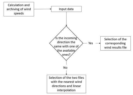
Figure 1.
Schematic representation of the algorithm for the prediction of the wind speeds.
The algorithm consists of the following steps:
- The wind speeds are calculated and archived for a specific computational field, for a number of distinct incoming wind directions (in the present test, 8 incoming wind directions have been considered to cover the entire 360° range).
- The user provides as input data the actual incoming wind direction.
- If the incoming wind direction coincides with one of the directions for which the wind speeds have been calculated, the algorithm selects the corresponding wind result file from the database. If not, then the two wind direction results files on both sides of the actual direction are retrieved and linear interpolation is applied to calculate the appropriate wind results file. It should be noted that linear interpolation is the simplest possible way to construct the intermediate wind field between two successive wind directions. Importantly, linear interpolation should work ideally when the distance between two successive wind directions is too small. More advanced methods based on, e.g., big data science and machine learning, will increase the efficiency of the present idea. These are concepts that will be examined by the authors in the future.
3. Governing Equations
The first step of the algorithm is to calculate and archive the wind speeds. In the present study, this step has been performed using RANS modeling. In RANS, the governing equations that are solved are:
where is the density, t is the time, ui are the velocity components, xi is the distance, P is the pressure, is the eddy viscosity, is the kinematic viscosity of the fluid, are the components of gravity acceleration, r is the gas constant, and T is the absolute temperature. The bar represents time-averaged values.
A considerable amount of work exists in the open literature concerning eddy viscosity modelling, especially in closed systems. The most advanced models in this area are those utilizing the turbulent kinetic energy k and the turbulent energy dissipation ε, obtained through transport equations or/and semi-empirical relations (e.g., [9]). The so-called standard k–ε model that has been extensively applied is based on the following transport equations for k and ε,
With constant values of , , , and .
4. The Pilot Test Case
In order to evaluate the algorithm, a computational field comprising a part of the atmospheric surface layer was selected. Figure 2 presents the selected field. The 3568 sensors of the MUST experiment (described below) were placed for this exercise to cover the area as much as possible (yellow circles). The height of the sensors ranged from 0.45 to 13.5 m.
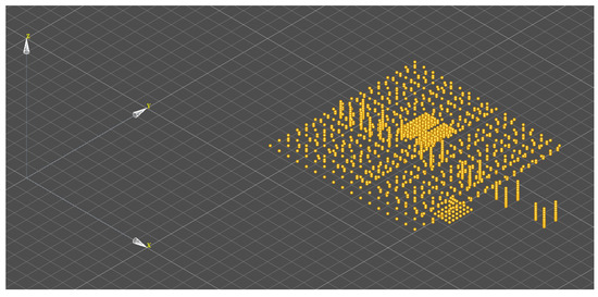
Figure 2.
The computational field that includes part of the atmospheric surface layer. The 3568 sensors are presented (yellow circles).
5. The Database
All the wind field calculations were performed with the CFD model ADREA-HF ([10]). The ADREA-HF model is a Eulerian model for the solution of the RANS and LES equations.
The database for the case under consideration includes the calculated flow fields from the ADREA-HF code for 8 incoming wind directions (0°, 45°, 90°, 135°, 180°, 225°, 270°, 315°) and a file with information about the computer grid. The size of the database for all wind directions is about 2 GB. The reference wind speed for all wind directions is equal to 8.3 m/s at a height of 10 m. It should be noted that in the present work the algorithm and the database are not designed to take into account different reference speeds, but there are thoughts in the future to use some kind of similarity in the speed distributions. Finally, neutral atmospheric conditions were applied and there is no effect on the results. Stable and unstable atmospheric conditions will be examined in the future.
Table 1 presents in detail the discretization of the computational field where almost 22.5 million cells have been used. The selection of the grid was performed on the one hand to be computationally manageable and on the other to be close to the grid of the MUST experiment presented in the work [11]. Recall that in the MUST experiment the horizontal dimensions of the field were approximately as in the present case (≈270 m) with a minimum cell size equal to 0.25 m in the horizontal and vertical direction. Moreover, regarding the ground boundary conditions, the lateral planes (inlet-outlet) for each of the 8 wind directions and the numerical methods, a similar strategy has been adopted as in the work [11].

Table 1.
Size of the selected computer field and numerical grid.
6. Validation of the Algorithm
The algorithm was validated for the present case for an incoming wind direction equal to 22.5° (non-existent in the database). The algorithm constructed the flow field using linear interpolation based on the flow fields of 0° and 45°. As we are dealing with hypothetical scenarios and there are no real measurements, an additional simulation for 22.5° was performed to generate synthetic flow data.
The performance of the algorithm for the 22.5° is presented in Figure 3 where, on the horizontal axis, the measurements of the synthetic simulation have been placed and, on the vertical axis, the values of the interpolation have been placed at the same measurement locations of the flow field (the velocity components u, v, w are presented). All data follow the ideal line 1 to 1, a fact that strengthens the good performance of the algorithm.
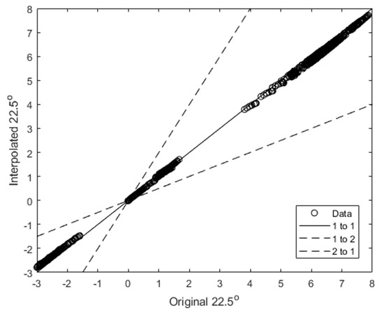
Figure 3.
Validation of the algorithm.
The execution time of the algorithm for the case of 22.5° (includes the reading time of the two files from the database and the interpolation time in the desired degrees) was calculated equal to be 3.06 min.
Given the duration of the 22.5° simulation is approximately equal to 15 h in 160 computing cores, it is obvious that the present methodology can be applied efficiently for emergency situations.
7. Validation of the Computer Code
7.1. The MUST Wind Tunnel Experiment
The correct operation of the algorithm presupposes that the computational fluid dynamics code accurately predicts the reality. For this reason, the code was validated with the data of the MUST wind tunnel experiment [12] given on a scale of the corresponding field experiment [13].
In the MUST experiment, the obstacles were placed in 12 rows, each consisting of 10 obstacles. The obstacles were almost similar and had length, width, and height equal to 12.2 m, 2.42 m, and 2.54 m respectively. The wind speeds were measured by the 3568 sensors presented in Section 3. It is noted that only the measurement data that were available to the authors (via the COST Action 732 database) are taken into account. The website for the COST Action 732 database is: https://mi-pub.cen.uni-hamburg.de/index.php?id=484 (accessed on 16 August 2021).
The wind tunnel measurements of the velocity components u, v and w were used to validate the numerical results of the hydrodynamic problem. Four sets of sensors were used corresponding to measurements in a coarse network, dense network, vertical profiles, and uw levels (Figure 4).
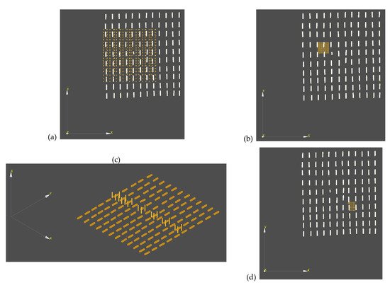
Figure 4.
The wind speed sensors (yellow circles) of the MUST wind tunnel experiment: (a) coarse network, (b) dense network, (c) vertical profiles, (d) uw levels. The 120 obstacles are also presented.
7.2. The Numerical Simulations
The size of the computational field is equal to 242.75 × 233.23 × 21.06 m on the x, y, and z axis respectively. The distance of the western boundary (left side of the field) from the first obstacle and the lateral boundaries from the obstacles is equal to 17.55 m (i.e., 5Hmax where Hmax = 3.51 m is the height of the tallest building) and the distance of the eastern boundary from the last obstacle is equal to 52.65 m (15Hmax). The height of the field corresponds to 6 times the maximum height of the buildings. These dimensions agree with the proposals of COST Action 732 [14].
The same grid presented in Table 1 was used to discretize the field. The height of the cells near the ground satisfies the minimum grid analysis proposed in the work [15], i.e., 1/10 of the height of the building of 2.54 m (Figure 5). Therefore, the field among the buildings has cubic cells and then continuously expands with a factor of 1.1. In the horizontal directions, the dx and dy are kept constant (Figure 5) in the field of obstacles covering an area of 172.55 m × 198.13 m. Outside the obstacle area, the dx and dy extend by a factor of 1.1.
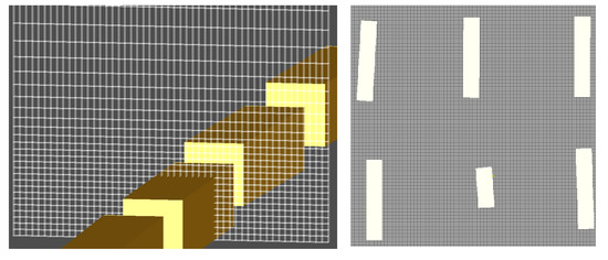
Figure 5.
Details of the grid: near the walls (left) and among the buildings (right).
For the LES simulations at the output of the flow a non-reflective boundary condition for the vertical velocity component was used as well as a zero-gradient boundary condition for the other velocity components. Wall functions for a rough wall were used on the surfaces of the buildings and the ground with a roughness length z0 equal to 10−5 m. At the inlet and top plane, a zero value was used as the boundary condition for the velocity components v and w while the Langevin type boundary condition was used for the velocity component u. Finally, as initial conditions, the vertical profile of the velocity of the mean flow imposed on the inlet was used throughout the field. For the RANS simulations, the same boundary conditions were used as in the work [11].
8. Validation of the Hydrodynamic Problem
The validation metrics (VMs) provide a quantitative way of comparing model predictions and measurements. The VMs are very useful for validating a model especially in the case of a large amount of data. Various VMs are available and each one has its advantages and disadvantages [14].
In the present study, the hit rate (HR) was used. The use of HR for the validation of microclimatic models was proposed by COST Action 732 [14]. The HR determines the fraction of the predictions that differ from the observations within an acceptable range given by the relative error D. The experimental uncertainty is taken into account with the parameter W, which expresses a “low value” limit.
The HR is calculated from the following equation:
where n is the total number of data, P is the model predictions, and O is the corresponding experimental observations. The minimum value of HR is 0 and the maximum is 1, which corresponds to a perfect agreement with the experiment. The parameter W is equal to 0.064 for the velocity component u and 0.056 for the velocity components v and w.
Table 2 presents the HR for the sensor groups presented in Figure 4. The number of sensors for each group is displayed in the parentheses. It is obvious that the results of RANS are similar to those of LES and except for component w the results of LES are slightly better. Moreover, the results of the component u which is the main component of the wind are better than the components v and w. Then the component v follows and finally the component w. According to COST Action 732, the acceptance criterion of HR is HR ≥ 0.66. It is observed that this criterion is satisfied for the horizontal components u and v for both methodologies (RANS and LES) and is not satisfied for the vertical component w.

In the literature, various models have been compared using the MUST wind tunnel experiment. For example, in the work [16], the HR of eight models, for 498 points (xz level), for the velocity component u ranged from 0.63 to 0.91 while for the velocity component w ranged from 0.12 to 0.26. The HR of the same velocity components of the simulations of the present work is within or even better than these ranges, indicating consistency with the results obtained from the work [16] and the corresponding one of COST 732 [14].
9. Conclusions
In this work, an algorithm was developed to predict the wind speed in renewable energy environments. The algorithm is based on CFD model results while at the same time it is fast enough to be applied in emergency situations. A wind speed database is calculated and stored in the preparation phase using a CFD model for the desired computational field and for a number of incoming wind directions. In a real event, the algorithm either selects the appropriate wind fields from the database, if the incoming wind direction coincides with one of the existing ones in the database, or calculates the wind field by interpolating from the nearest wind directions in the database. The above procedure performed in the case of an event (i.e., acquisition of the wind field from the database, possible interpolation) is fast and suitable for application in emergency situations.
The test case used in this work to evaluate the algorithm is a computational field that includes part of the atmospheric surface layer. The wind fields were calculated for eight incoming wind directions covering the entire 360° range. The CFD code ADREA-HF was used in this study to calculate the flow fields and the synthetic flow field of 22.5° (not included in the precalculated database) as we treat hypothetical scenarios. The algorithm showed satisfactory operation. The solution was obtained in a short execution time (less than 5 min), which indicates the suitability of the algorithm for critical response. It should be noted that the present algorithm is new and is applied in this paper for the first time. Future efforts will be performed to achieve further results of applications of the algorithm in renewable energy environments.
Finally, the suitability of the CFD code was evaluated with additional simulations of the MUST wind tunnel experiment. The numerical results of two turbulence methodologies (RANS and LES) were compared with the respective experimental measurements of the velocity components u, v, and w. The validation metric HR is good and is satisfied in the case of components u and v. For the velocity w, the HR is better than the results of the literature.
Author Contributions
Conceptualization, methodology, validation, writing, G.E.; review, supervision, F.B., and N.M.; review, G.T. All authors have read and agreed to the published version of the manuscript.
Funding
This research received no external funding.
Acknowledgments
The simulations were supported by computational time granted by the Greek Research & Technology Network (GRNET) in the National HPC facility ARIS (http://hpc.grnet.gr) under project CFD-RI (pr008008). Present authors would like to thank Tolias Ilias from NCSR Demokritos for giving permission to use the MPI version of ADREA-HF. Present authors would like to thank all members of COST Action 732 (https://mi-pub.cen.uni-hamburg.de/index.php?id=484).
Conflicts of Interest
The authors declare no conflict of interest.
References
- Seshaiah, C.V.; Sukkiramathi, K. A Mathematical model to estimate the wind power using three parameter Weibull distribution. Wind. Struct. 2016, 22, 393–408. [Google Scholar] [CrossRef]
- Chiodo, E.; De Falco, P. Inverse Burr distribution for extreme wind speed prediction: Genesis, identification and estimation. Electr. Power Syst. Res. 2016, 141, 549–561. [Google Scholar] [CrossRef]
- Tolias, I.C.; Koutsourakis, N.; Hertwig, D.; Efthimiou, G.C.; Venetsanos, A.G.; Bartzis, J.G. Large Eddy Simulation study on structure of turbulent flow in a complex city. J. Wind Eng. Ind. Aerodyn. 2018, 177, 101–116. [Google Scholar] [CrossRef] [Green Version]
- Coceal, O.; Goulart, E.V.; Branford, S.; Thomas, T.G.; Belcher, S.E. Flow structure and near-field dispersion in arrays of building-like obstacles. J. Wind Eng. Ind. Aerodyn. 2014, 125, 52–68. [Google Scholar] [CrossRef] [Green Version]
- Koutsourakis, N.; Bartzis, J.G.; Markatos, N.C. Evaluation of Reynolds stress, k-ε and RNG k-ε turbulence models in street canyon flows using various experimental datasets. Environ. Fluid Mech. 2012, 12, 379–403. [Google Scholar] [CrossRef]
- Berchet, A.; Zink, K.; Muller, C.; Oettl, D.; Brunner, J.; Emmenegger, L.; Brunner, D. A cost-effective method for simulating city-wide air flow and pollutant dispersion at building resolving scale. Atmos. Environ. 2017, 158, 181–196. [Google Scholar] [CrossRef]
- U.S. Naval Research Laboratory. CT-Analyst. Available online: https://www.nrl.navy.mil/Our-Work/Areas-of-Research/Computational-Physics-Fluid-Dynamics/CT-Analyst/ (accessed on 7 December 2021).
- Leitl, B.; Hertwig, D.; Harms, F.; Peeck, C.; Schatzmann, M.; Patnaik, G.; Boris, J.; Obenschain, K.; Fischer, S.; Rechenbach, P. Emergency Response Tool for Accidental Releases; Short Course on Urban and Technical Meteorology (Lecture Notes), Universidad National de Colombia: Bogota, Colombia, 2012. [Google Scholar]
- Launder, B.E.; Reece, G.J.; Rodi, W. Progress in the development of a Reynolds-stress turbulence closure. J. Fluid Mech. 1975, 68, 313–348. [Google Scholar] [CrossRef] [Green Version]
- Bartzis, J.G. ADREA-HF: A Three Dimensional Finite Volume Code for Vapour Cloud Dispersion in Complex Terrain; CEC JRC Ispra Report EUR 13580 EN; EC Joint Research Centre: Ispra, Italy, 1991. [Google Scholar]
- Efthimiou, G.C. Prediction of four concentration moments of an airborne material released from a point source in an urban environment. J. Wind Eng. Ind. Aerodyn. 2019, 184, 247–255. [Google Scholar] [CrossRef]
- Bezpalcova, K.; Harms, F. EWTL Data Report/Part I: Summarized Test Description Mock Urban Setting Test; Technical Report; Environmental Wind Tunnel Lab. Center for Marine and Atmospheric Research, University of Hamburg: Hamburg, Germany, 2005. [Google Scholar]
- Yee, E.; Biltoft, C. Concentration fluctuation measurements in a plume dispersing through a regular array of obstacles. Bound.-Layer Meteorol. 2004, 111, 363–415. [Google Scholar] [CrossRef]
- Schatzmann, M.; Olesen, H.; Franke, J. Model Evaluation Case Studies: Approaches and Results. COST Action 732 Quality Assurance and Improvement of Microscale Meteorological Models; University of Hamburg: Hamburg, Germany, 2010; ISBN 3-00-018312-4. [Google Scholar]
- Tominaga, Y.; Mochida, A.; Yoshie, R.; Kataoka, H.; Nozu, T.; Yoshikawa, M.; Shirasawa, T. AIJ guidelines for practical applications of CFD to pedestrian wind environment around buildings. J. Wind Eng. Ind. Aerod. 2008, 96, 1749–1761. [Google Scholar] [CrossRef]
- Tominaga, Y.; Iizuka, S.; Imano, M.; Kataoka, H.; Mochida, A.; Nozu, T.; Ono, Y.; Shirasawa, T.; Tsuchiya, N.; Yoshie, R. Cross comparisons of CFD results of wind and dispersion fields for MUST experiment: Evaluation exercises by AIJ. J. Asian Architect. Build Eng. 2013, 12, 117–124. [Google Scholar] [CrossRef] [Green Version]
Publisher’s Note: MDPI stays neutral with regard to jurisdictional claims in published maps and institutional affiliations. |
© 2021 by the authors. Licensee MDPI, Basel, Switzerland. This article is an open access article distributed under the terms and conditions of the Creative Commons Attribution (CC BY) license (https://creativecommons.org/licenses/by/4.0/).