Abstract
Improving indoor air quality and energy consumption is one of the high demands in the building sector. In this study, unsteady flow oscillations in a 3-D ventilated model room with convective heat transfer have been studied for three configurations of an empty room (case 1), a room with an unheated box (case 2) and a room with a heated box (case 3). Computational results are validated against experimental data of airflow velocity, temperature and turbulence kinetic energy. For each case, flow unsteadiness is presented by the time history of airflow velocity and temperature at prescribed monitor points and further analyzed using the Fast Fourier Transform technique. For case 1, the flow oscillation is irregular and less dependent on the monitor points. For case 2, the flow oscillation is still irregular but with increased frequency, possibly due to enhanced flow recirculation around the corners of the unheated box. For case 3, a dominant frequency exists, and thermal energy oscillating is higher than flow kinetic energy. Among the three cases, case 3 has the highest dominant frequency in a range of 4.3–4.6 Hz, but the kinetic energy is the lowest at 1.25 m2⁄s. The unsteady flow oscillation is likely due to a high Grashof number and corner flow recirculation for cases 1 and 2, and a combination effect of a high Grashof number, corner flow recirculation and thermal instability (induced by the formation and movement of the thermal plume) for case 3.
1. Introduction
In a 3-D ventilated indoor space, such as a room, airflow movement continuously occurs due to the combination effects of forced incoming cooling flow and natural thermal buoyancy. At high Reynolds number turbulent flow conditions, the airflow pattern could be very complicated, particularly with the appearance of flow unsteadiness and velocity/temperature field oscillations. Despite its existence, there is a very limited number of published works available about the analysis and discussion of the flow unsteadiness phenomenon and its underlying thermophysical mechanisms within the context of an indoor environment. One relevant attempt in the past was to correlate the velocity fluctuation with occupant discomfort [1], and it was found that the discomfort would reach a maximum level whilst a velocity fluctuation frequency was in a range of . Some researchers also claimed from their experimental studies that a velocity oscillation associated with higher turbulence kinetic energy (KTE) occurred in a low frequency range of for a ventilated space with/without thermal loads [2], and in some cases the frequency band could be higher, up to , in ventilated spaces without thermal loads [3]. Based on a study of a natural convection in a square cavity [4], researchers also observed some uncorrelated oscillation frequencies between the velocity and temperature fields, and these oscillations were mainly developing along the flow direction between the hotter and colder isothermal walls. For natural convection flows in a tall cavity, numerical studies revealed a characteristic frequency of [5] and turbulent flow fluctuations near the core of the flow circulation [6], possibly due to strong asymmetrical flow motions together with a high level of heat transfer. For flow oscillation in a mixed convection scenario, such as a prescribed heat source located on a vertical wall in a ventilation system, a correlation between the Reynolds number () and the Grashof number () was also found for conditions of and [7]. In a more realistic indoor environment, such as ventilated spaces with occupants, it was found that the mean airflow velocity can increase with the decrease of turbulence intensity and the domain height [2,3,8]. Despite the existence of flow oscillations observed in various experimental and numerical studies, as described above, the causes and underlying thermophysical mechanisms are still unclear. Some researchers have argued that it could be related to flow and thermal instabilities that can be induced by the thermal conductivity of boundaries [9], the strength of the buoyancy effect [10] or the wall-bounded boundary layers along the solid wall and the 3-D corner effects [4]. Some recent studies in the field include a CFD simulation in a naturally ventilated room with a localized heat source [11], a comprehensive review of unsteady room ventilation [12] and an optimization study on indoor building energy consumption in relation to passive design and alternative energy [13]. Although these studies revealed some relations between flow oscillation and thermal instability, there is still lacking detailed and in-depth analysis on flow unsteadiness in relation to the flow and thermal fields as well as further instability analysis. This forms the motivation of the present study.
Various methods are used to study flow and heat transfer phenomena in an indoor environment. Among them, the traditional approach of building a dedicated physical test room to perform field measurements of key parameters such as velocity and temperature time history would be ideal, as it is vital in providing reliable and real-time reference data for indoor environment design engineers. However, this process is very time consuming and expensive, in addition to the other limitations of real-time data acquisition and measurement, such as the change/control target flow and thermal conditions. In recent years, the computational fluid dynamics (CFD) technique has demonstrated its capability in capturing detailed real-time information of 3-D complex flow and heat transfer characteristics accurately at both system and component levels. Moreover, it is able to carry out an efficient postprocessing analysis of a large amount of information obtained from simulations, which has to be dealt with in an accurate, cost-effective and time-saving manner during the building thermal design and assessment processes. Thus, the present study applies the CFD technique to simulate flow and heat transfer phenomena in an indoor environment.
As described above, one major challenge of studying flow oscillation phenomena in an indoor environment was that there is a lack of available detailed information, e.g., the level of kinetic energy oscillations, the flow fluctuations and their variations across the entire domain of interest, to be used for research and analysis. This is partly due to the fact that vast amounts of time history data were based on on-site measurements [4]. Hence, it is difficult for indoor engineers to realize the characteristics of flow unsteadiness and to consider and implement it in their design practices. To overcome this problem, the present study aims to investigate the origin and the development of flow oscillation in a 3-D ventilated model room with an increased complexity of flow and thermal features by introducing a cubic box without and with thermal loads. The phenomenon of flow oscillation will be studied, as well as the correlation and the characteristics of the associated flow and heat transfer. The employed mathematical model and numerical scheme will be carefully tested and validated against available experimental data [14], and the flow unsteadiness will be analyzed using the Fast Fourier Transform (FFT) technique.
2. Numerical Methods
2.1. Governing Equations
The fluid flow and heat transfer are governed by a set of conservation equations (mass, momentum and energy). The Reynolds-averaged Navier–Stokes (RANS) equation is adopted for turbulent flows. These equations can be expressed in a general Cartesian form as follows:
Mass conservation equation
Momentum conservation equation
Energy transport equation
where is time, is density (), is partial differentiation operator, is velocity vector, is pressure (), is gravitational body force vector and is other external body force vector, is total energy (), is effective heat conductivity (), is temperature, is sensible enthalpy, (), is specific heat at constant pressure , is diffusion flux of species , is effective stress tensor and is an additional energy source due to chemical reaction or radiation. The term of is written as
where is viscosity (), is matrix transpose, is unit tensor and is the Reynolds stress term for turbulent flow (, where is the Reynolds stress tensor).
2.2. Prediction of Airflow and Heat Transfer
CFD software ANSYS Fluent is utilized to calculate airflow and thermal property distributions in a 3-D ventilated model room based on the governing continuity, momentum and energy equations described above. The Reynolds-averaged Navier–Stokes (RANS) equations are adopted together with the two-equation renormalized group RNG k-ε turbulence model, due to its capability of accurate prediction of indoor turbulent airflows at a moderate-to-high Grashof number with and without flow swirl. Some previous studies have shown favorite performances of this model in terms of its accuracy and stability and shorter computing time [15,16]. The complete formulation of all equations used in this study can be found in a recent publication by the present authors [17]. This study will be further extended to include a more sophisticated six-equation Reynolds Stress turbulence model to show the discrepancies of the two turbulence model results in comparison with the test data.
An iterative solution method, the SIMPLE algorithm [18], is employed to solve the nonlinearity of the momentum equation, the velocity–pressure coupling and also the coupling between the flow momentum and the energy equations. For the pressure Poisson equation, the solution applies weighted body force under the assumption that the gradient of the difference between the pressure and the body forces remains constant, especially in the buoyancy calculations. Other equations, such as momentum, energy and radiation, are solved using the second-order numerical scheme. Double precisions are always defined to have better numerical accuracy, and the residual target is set as to achieve a high level of convergence.
2.3. Fast Fourier Transform
The Fast Fourier Transform (FFT) technique is used to analyze the flow unsteadiness and oscillations in a 3-D ventilated model room based on CFD-predicted time history data (e.g., velocity and temperature) obtained from ANSYS Fluent software at prescribed monitor locations and from a corresponding experiment. Another method, the Discrete Fourier Transform (DFT), as shown below, is also used to reduce the computing time from an order of to for a given set of points (see, e.g., Cooley and Tukey [19]). In the present study, a Matlab program using the FFT technique is developed to calculate the frequency spectrum (FS) and the power spectral density (PSD) of flow oscillations. The DFT method is described as:
with
By splitting Equation (5) into two parts:
Then, the Fast Fourier Transformation (FFT) is described as
where
All notations and symbols used in equations above are standard and can be found in public domain, as well as some textbooks, e.g., Smith [20].
3. Physical Problem
The problem of airflow inside a 3-D ventilated model room represents one of the most common flow and heat transfer scenarios in an enclosed indoor environment. In addition to some general 3-D flow characteristics, such as velocity and temperature distributions, the particular focus of the present study will be the unsteady flow pattern and its temporal/spatial variations caused by the presence of an unheated box at the center of the domain. Furthermore, the formation and development of the thermal plume and natural buoyancy flow from a heated box. In all three cases studied, the flow oscillation and its possible causes will be analyzed and discussed in detail.
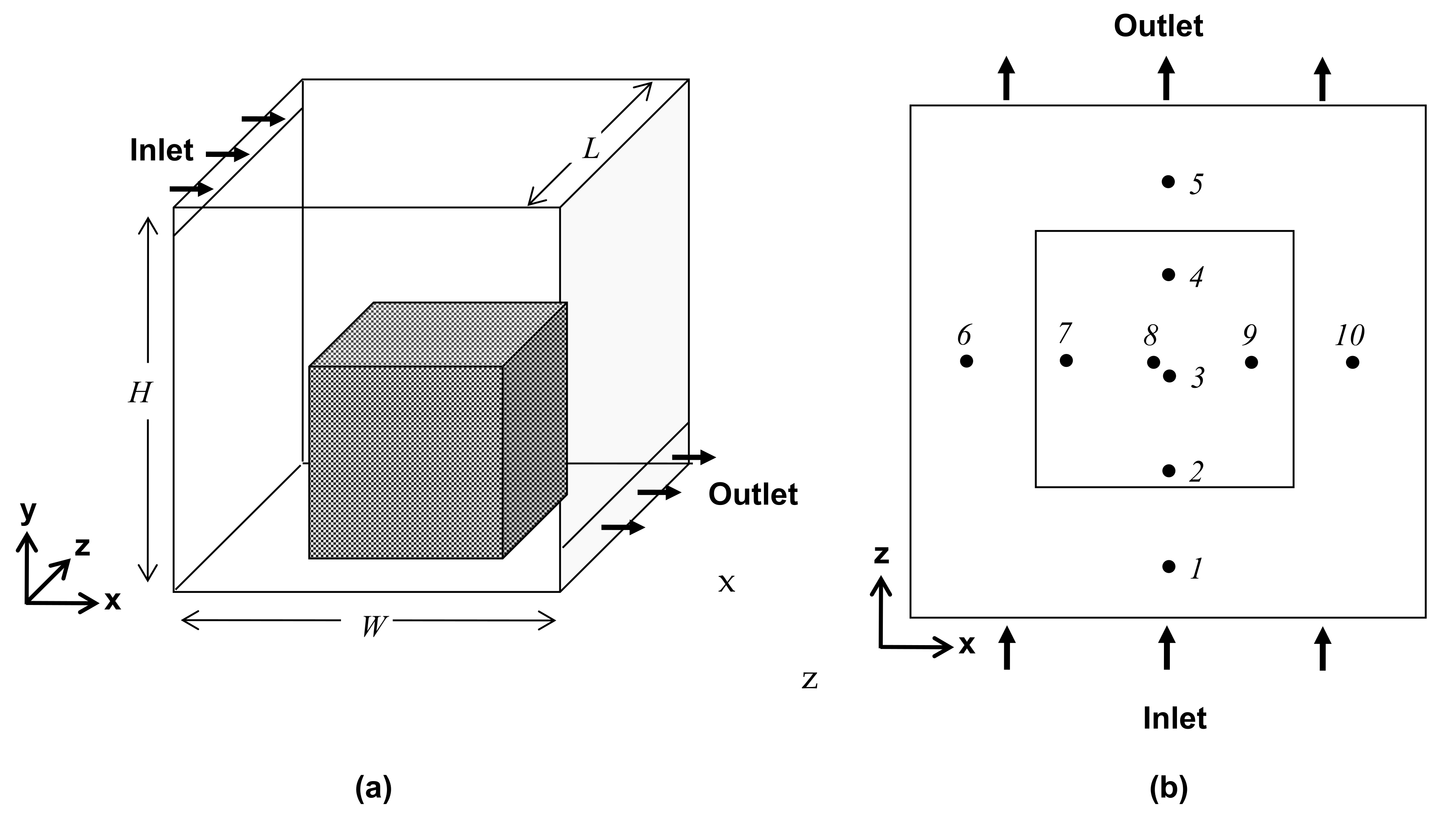
The 3-D model room experimentally studied by Wang and Chen [14] are chosen in present study, considering the three configurations as an empty room (case 1), a room with an unheated box (case 2) and a room with a heated box (case 3), respectively. For cases 2 and 3, a smaller cubic box by a factor of 2 in all three dimensions is located at the center of the model domain on the floor (see Figure 1). Table 1 gives a summary of the three cases and their corresponding flow and heat transfer models.

Figure 1.
Sketch of a 3-D ventilated model room of 2.44 m × 2.44 m × 2.44 m in dimensions. (a) Inlet/outlet slots and a small cubic box; (b) Positions of ten measurement lines.

Table 1.
Summary of all three cases in a three-dimensional model room.
The 3-D cubic model room studied has an edge length of in all three dimensions, an inlet slot ( in height, 2.44 m in width) attached to the ceiling at the front wall and an exit slot ( in height, 2.44 m in width) attached to the floor at the back wall, as seen in Figure 1. In case 2, a small unheated cubic box with an edge length of is located at the center of the room on the floor (see Figure 1), and in case 3, the box is heated, generating a heat source of Watts, which is equivalent to in terms of the temperature uniformly distributed around the box surfaces. For all three cases, there is an incoming airflow at a flow rate of and an ambient temperature of , respectively. Based on the thermophysical condition of the model room and the heated box, it is estimated that and , where is the Grashof number and is the Reynolds number, respectively. Hence, the heat transfer due to the forced convection mode will play a major role in the flow and heat transfer process compared to that of the merely natural convection mode.
The problem is solved by a finite volume numerical method on uniformly structured grids. A grid independent study is conducted using Cartesian coordinates (, and ) on two successive grid resolutions of and points nonuniformly distributed in the domain, and a grid independent solution was achieved with a grid of . Further details on the grid refinement study can be found in references [15,17].
Unsteady flow simulations are carried out using a fixed time step of , determined by the smallest mesh size divided by the inflow air velocity, i.e., the smallest flow convective time. After the initial transient stage, the time-averaged ‘mean’ results are then calculated based on a total of successive datasets, each averaging over time steps during the calculation. Finally, the averaged results from the unsteady calculation, such as the flow velocity, temperature and turbulence kinetic energy (,), are compared with the available experimental data obtained by Wang and Chen [11]. The flow velocities are normalized by the maximum inlet velocity, , and the turbulence kinetic energy normalized by the maximum value of . For the temperature normalization in case 3, a formula of is used with , i.e., the air temperature at the inlet slot, and , i.e., the surface temperature of the heated box, as reference values, respectively.
In order to compare with the available experimental data in terms of air velocity, temperature and turbulence kinetic energy (TKE), a total of 10 monitoring positions on a streamwise midplane and a spanwise midplane are defined, as shown in the filled-circle marks in Figure 1b, with their coordinates given in Table 2. It can be seen that for cases 2 and 3, with a small cubic box, there are four measurement lines around the box, and for the rest, six lines are above it. For each case, the results of the flow velocity, temperature and turbulence kinetic energy distributions at the five representative monitoring/measuring positions are shown in order to illustrate the level of accuracy in comparison with the measurement data.
Table 2.
Positions of ten measuring lines.
4. Validations
Turbulence Model Effects
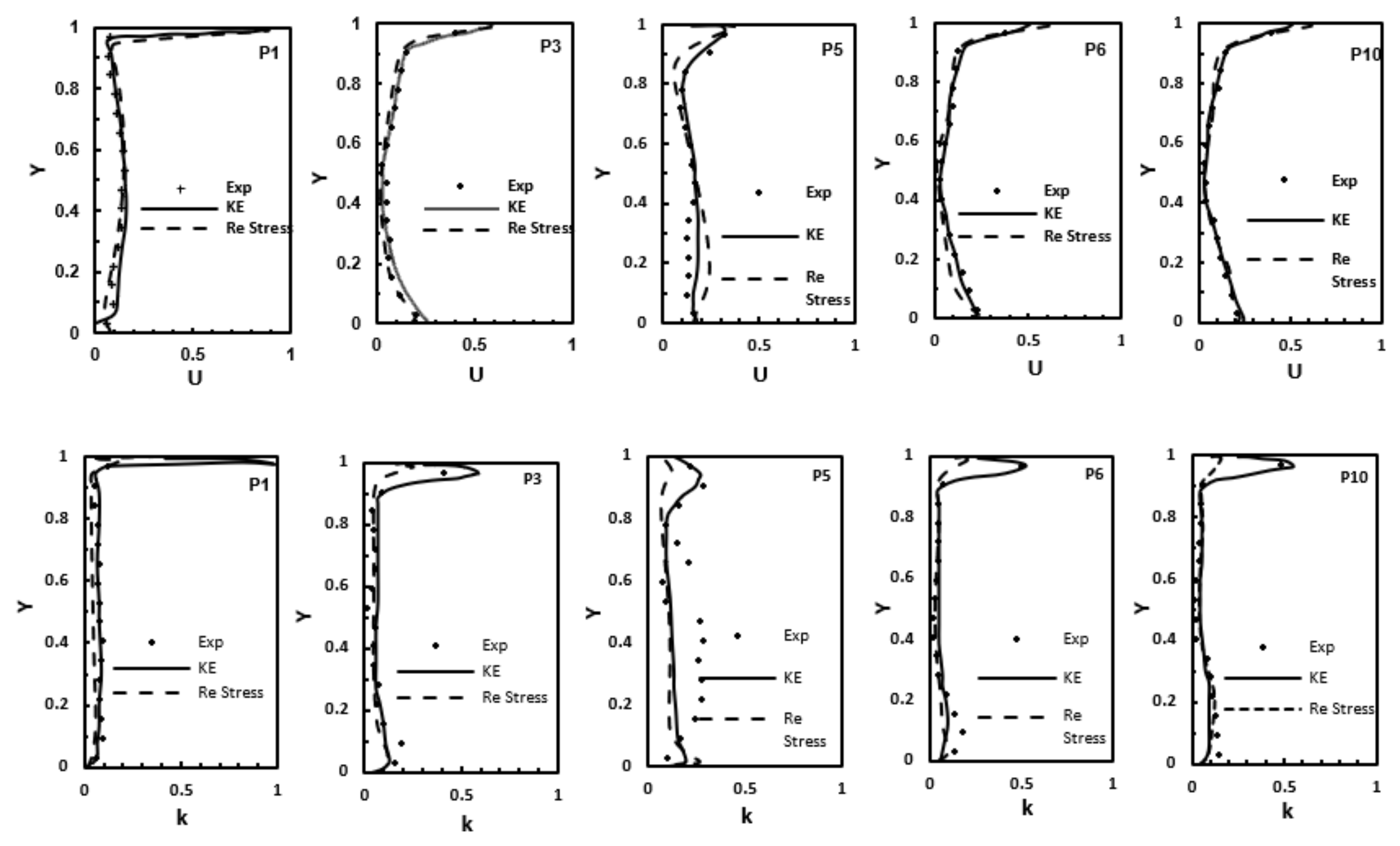
The case 1 study has been used to compare the results from the six-equation Reynolds Stress model and the two-equation RNG k-ε turbulence model for model performance assessment, such as accuracy and efficiency. Figure 2 depicts the normalized time-averaged (mean) velocity and turbulence kinetic energy (TKE) profiles at five monitoring points from these two turbulence models in comparison with experimental data [14].

Figure 2.
Comparison of normalized velocity and turbulence kinetic energy profiles at monitoring points 1, 3, 5, 6 and 10 for case 1, predicted by the RNG k-ε and the Reynolds Stress turbulence models, respectively.
It is clear that the Reynolds Stress model does not produce more accurate results than the RNG k-ε turbulence model. The most discrepancies between the numerical predictions and experimental data were observed at the lower or upper part of the flow domain away from the center of the domain. In fact, the RNG k-ε model-predicted normalized U-velocity profiles at points 5, 6, 10 are in better agreement with test data than the Reynolds Stress model, as the latter gives undesirable predictions in regions close to the upper wall. In general, the RNG k-ε turbulence model has achieved overall better performance in terms of accuracy, efficiency and less computational cost, and this observation agrees well with other published studies [15,16]. Hence, the following study of all three cases will only use the RNG k-ε turbulence model (denoted as ‘Model’ thereafter).
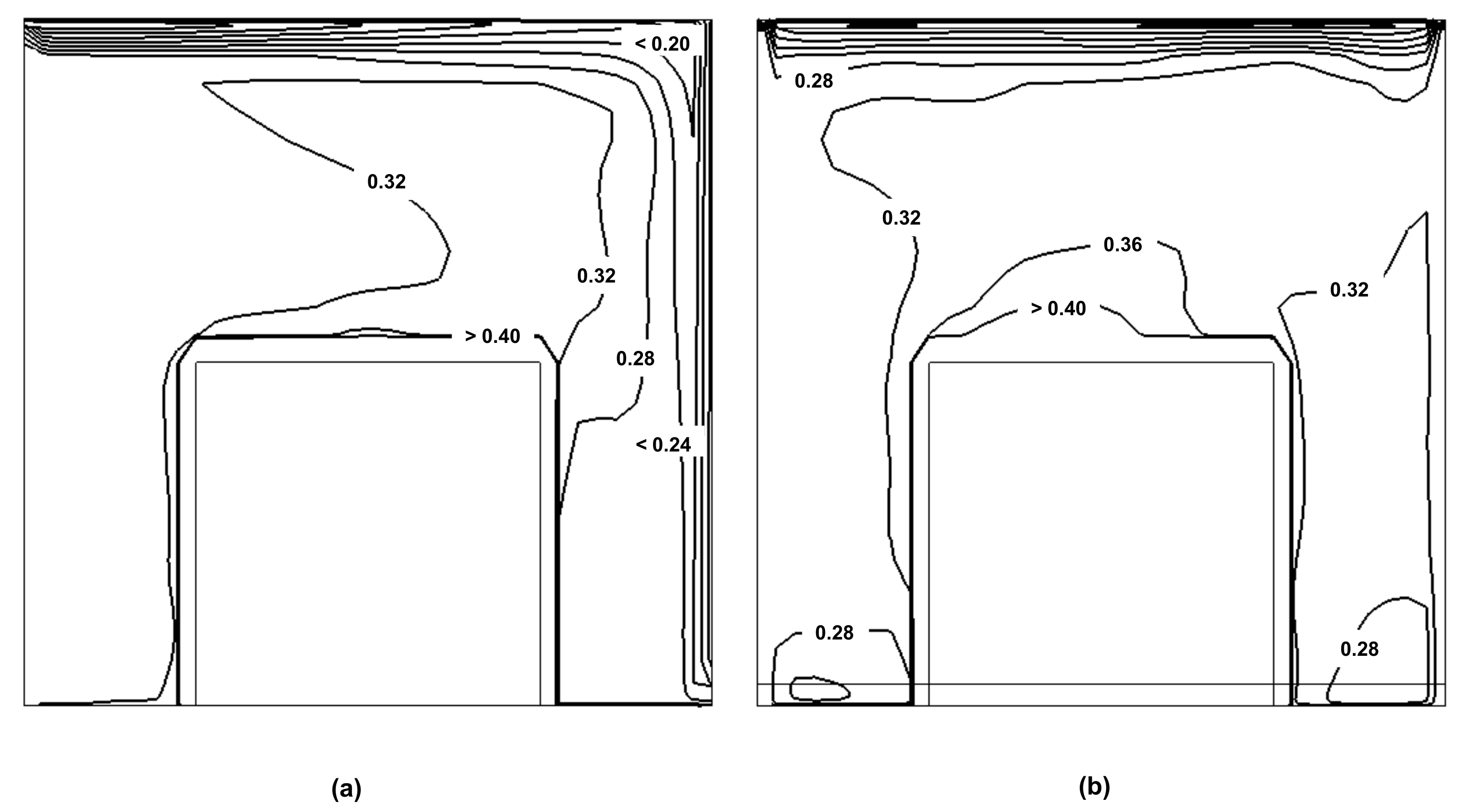
Figure 3 illustrates the contours of instantaneous velocity magnitude and turbulence kinetic energy (TKE) at 20,000 iterations, both normalized by its reference values, as described above, on a streamwise mid-plane (x, y, z = L/2) for cases 1–3. It can be seen that in an empty room domain (case 1), a large clockwise flow recirculation is formed, stretching almost diagonally across the entire domain from the top-right corner to the bottom-left corner. The flow velocity increases to a maximum value in the near-wall regions, while it decreases to a minimum value close to the center of the room. The presence of an unheated box (i.e., case 2) induces flow separation around the sharp leading-edge of the small cubic box, causing two large-scale flow recirculation structures. They are (1) a near-vertical structure inside the gap between the box’s rear surface and the domain back wall, and (2) a near-diagonal structure on the top of the box extending to the top-right corner, respectively. The flow recirculation above the box is found changing with time in terms of the flow pattern and recirculation size. With the heated box (case 3), the flow recirculation has been further enhanced, especially the one formed at the front of the box and the other vertically in the rear of the box, possibly due to the strong thermal buoyancy effects between the heated box surfaces and the adjacent domain walls. The corresponding TKE contours show a low level of magnitude across the mid-plane in case 1, except for the jet stream path along the ceiling. In case 2, the appearance of a vertical recirculation slightly enhanced the TKE, with the increased range (e.g., almost doubling the streamwise length) of the TKE higher than 0.1. In case 3, the strong buoyancy effect largely promotes the TKE at the rear of the heated box (see Figure 3f), where the TKE is greater than 0.4 over a large area, and this somehow restricts the development of the cold jet stream, resulting in a much shorter streamwise distance of the TKE, higher than 0.1 compared to that of case 2. The normalized temperature field from the case 3 (as shown in Figure 4) indicates that there is a large thermal plume formed and developed from the top surface of the heated box, resulting in temperature gradient increase near the domain walls (see Figure 4a). The higher temperature gradient will likely lead to an unstable stratification effect in an alignment with the cold inlet ‘jet’ stream flow along the streamwise direction. In a spanwise plane (see Figure 4b), the temperature distribution is found to be almost symmetrical.
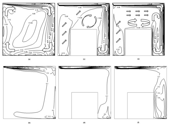
Figure 3.
Contours of normalized velocity (top) with superimposed sketches of flow stream pattern and turbulence kinetic energy (bottom) on a streamwise midplane (x, y, z = L/2) for three cases (i.e., (a,b) case 1, (c,d) case 2 and (e,f) case 3, respectively).
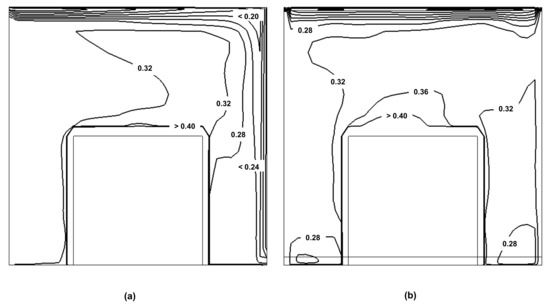
Figure 4.
Contours of normalized temperature on mid-plane in (a) streamwise direction and (b) spanwise direction for case 3.
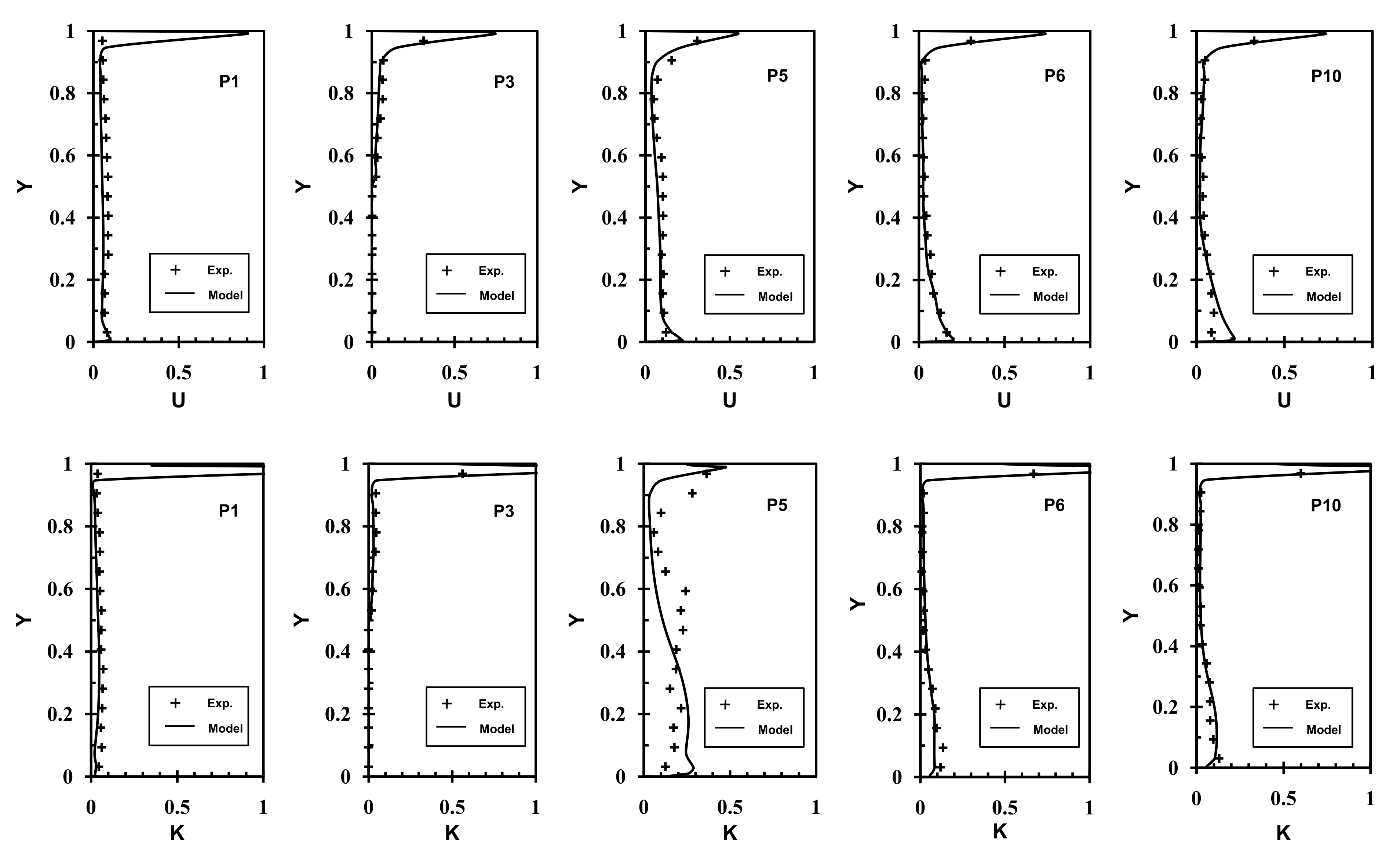
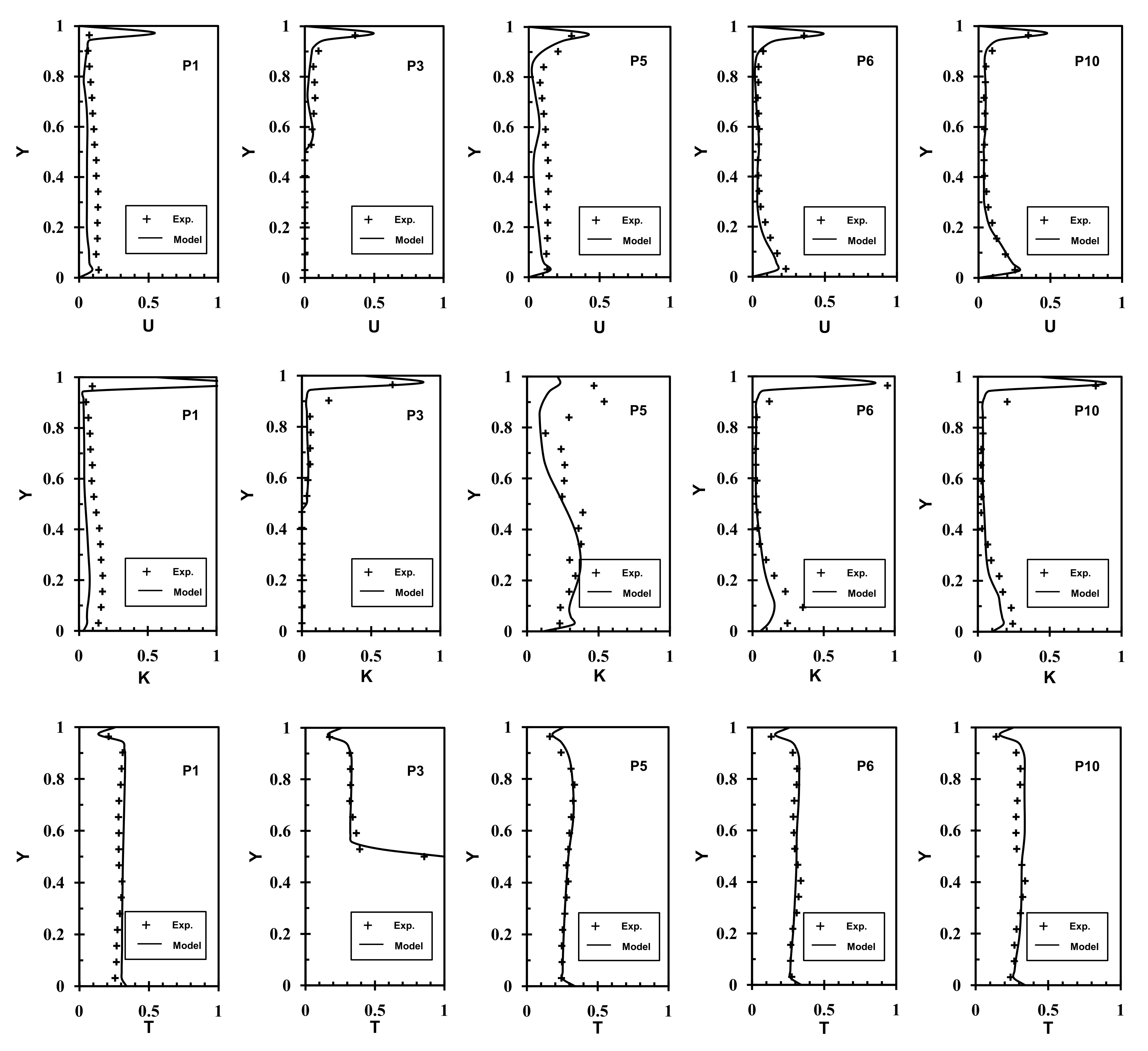
Figure 5 and Figure 6 depict the normalized numerical prediction results of time-averaged velocity, turbulence kinetic energy and temperature (for case 3 only) at five selected monitoring points for cases 1–3 compared with the available experimental data [14]. It can be seen that, in general, the velocity near the ceiling decays fairly quickly along the distance from the inlet opening to the downstream locations, while the velocity in the floor near-level shows a clear peak in magnitude at three mid-spanwise locations (i.e., , and ). Comparing to the domain with unheated or heated box (i.e., case 2 and case 3), the velocity magnitude in an empty model room (i.e., case 1) increases to a high level. For example, in case 1, the velocity magnitude increases to its value around the mid-height Y at and , whereas it decreases to its value at the locations on the midspanwise plane, , and . In case 2 and case 3, on the other hand, this trend of velocity magnitude change is not seen, i.e., no large velocity develops in the upper region along the vertical domain height (Y). The TKE distributions show only a noticeable development along the ceiling from the inlet and a slight increase in the lower levels (i.e., ) of the domain height for all the cases. The major discrepancies between present results and the experiment are seen at through the domain height. Note that TKE is often associated with larger uncertainties and errors in both the CFD and the experiment, as previously discussed [21]. In case 3 of a heated box, the present results slightly underpredict the velocity and TKE values at positions of and in the region of and the positions of and in the region of . It can be seen that there are rapid declines in TKE from locations to , which leads to some underestimations of TKE at . In terms of temperature, the present results are all in good agreement with the measurements at all the locations.
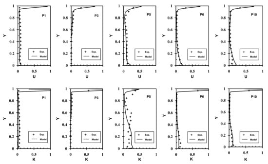
Figure 5.
Comparison of normalized velocity and turbulence kinetic energy profiles at monitoring points 1, 3, 5, 6 and 10 for case 2.
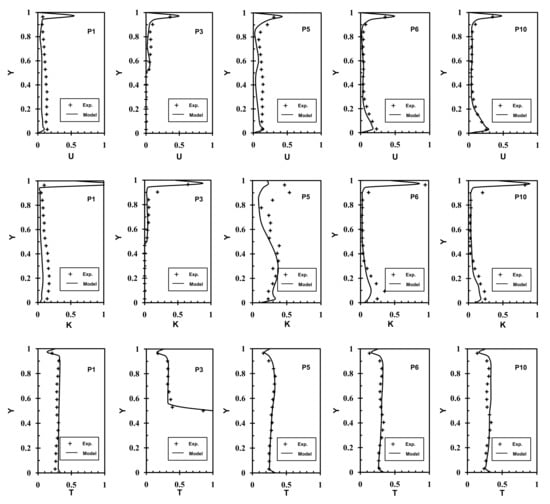
Figure 6.
Comparison of normalized velocity, turbulence kinetic energy and temperature profiles at monitoring points 1, 3, 5, 6 and 10 for case 3.
Based on the results obtained for the three case studies above, it can be concluded that the increase of the complicity of the geometry features (i.e., from an empty model room to the same model room with a box with/without heating in the domain) lead to flow separation around the sharp edges of the box, accompanied by large-scale flow recirculation above the box and in the rear-space of the domain, in addition to some flow swirls in the front-space, respectively (see, e.g., Figure 3a,c,e). It is found that the presence of an unheated box (case 2) reduced the velocity magnitude by about 5% in a region above the box at the center of the domain (P3) and 28% at the other measuring locations, as defined in Table 2, compared to those predictions of an empty room. However, TKE is found to have increased by 13–25% at P5, P6 and P10, and decreased at P1 by 30%, when compared to an empty room in case 1. For case 3, the strong thermal buoyancy effect weakens the velocity magnitude and TKE by 40–70% at all the measuring locations, except for that at the P5 location, where the TKE has been surprisingly increased by 46%. The reason for this large change is not fully understood yet.
5. Results and Discussion
In a reference paper [15], the adopted mathematical models along with the numerical schemes were described and comprehensive numerical experiments and validations against available experimental data [14] were made. Based on the FFT analysis of the time history of the flow field data, it was found that both the airflow velocity (case 1) and the temperature (case 3) oscillate at a very low frequency up to . While the reason is still unclear, it suggested that the origin of the flow unsteadiness might be due to a combination of a high Grashof number flow and thermoconvective instability of the ‘hot’ fluids lying beneath the ‘cold’ fluids, leading to a significant buoyancy effect inside the domain. The present study continues that investigation by applying the FFT analysis to those obtained unsteady CFD data in order to understand the underlying thermophysical mechanisms related to the observed flow unsteadiness.
For all three case studies, unsteady flow simulation starts from a uniform flow field at a fixed time step (0.055 s), defined by the minimum cell size and convective airflow velocity at the inlet slot location. After the initial transient stage, and until the ‘statistically-converged’ status is reached, the time history of the airflow velocity magnitude (for all three cases) and temperature (for case 3 only) at the five prescribed monitoring locations , , , , and normalized heights , , , , were stored for every iterations/time steps over a sufficiently large-size sample data. The accumulated time history data are then analyzed by an in-house Matlab FFT program based on the predicted time history data at those monitoring locations and heights. The results are then to be compared with available experimental data, in particular the oscillation frequencies.
5.1. Oscillation Signals
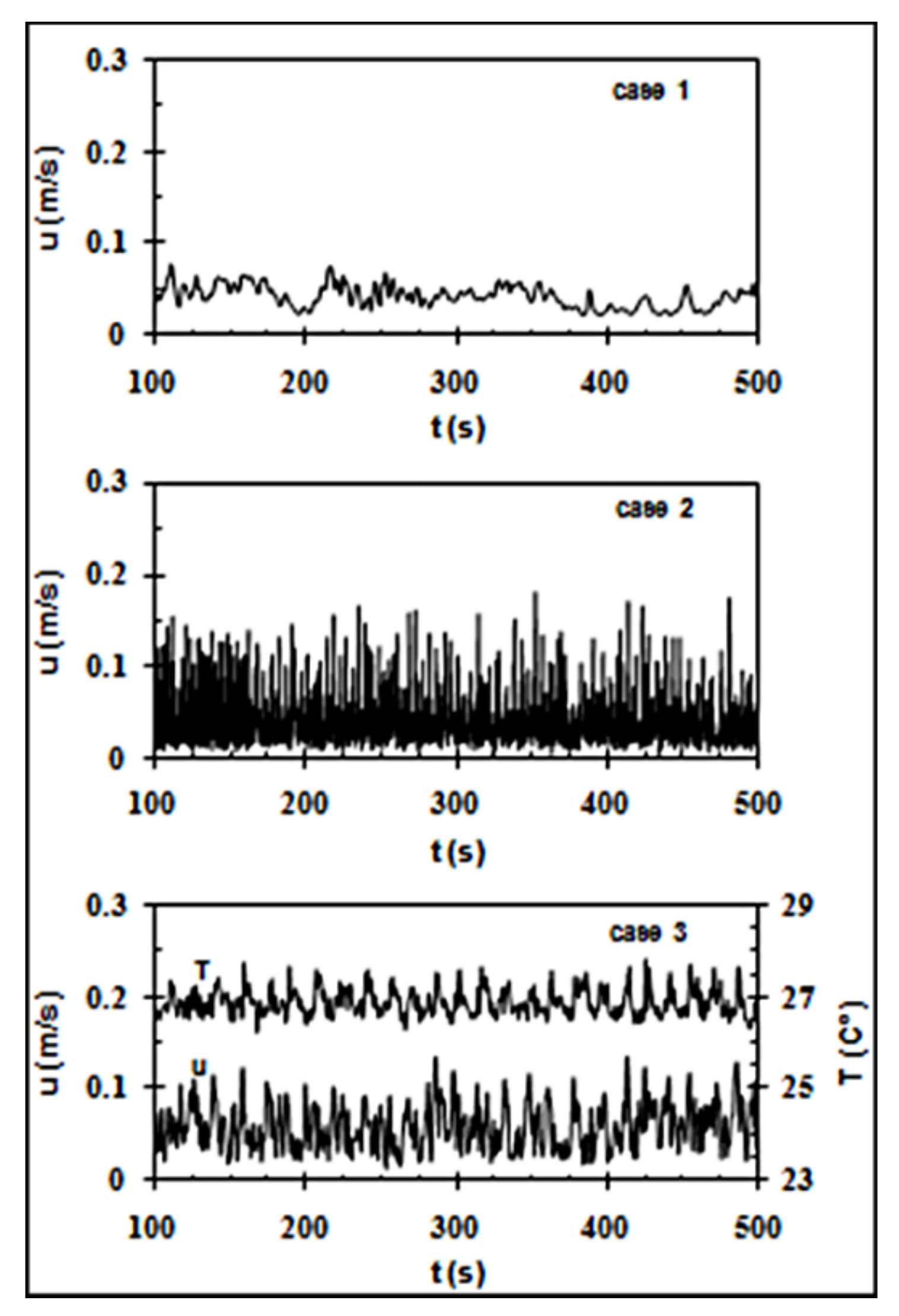
Figure 7 shows both the velocity and temperature fluctuation signals during a time period of at of for all three cases. The results at the other locations are also analyzed (though not presented here). Based on the prescribed time step and an inlet velocity , this time period of the simulation is equivalent to complete flow recirculation cycles. It can be seen that there is no particular trend or similarity in fluctuation variations among these three cases and the amplitude of the spikes is generally asymmetric. The fluctuation variation in case 1 seems smaller, e.g., in a range of , compared to that of case 2 and case 3, for which the range of the velocity fluctuation is relatively larger, i.e., . The presence of the unheated box in the domain (i.e., case 2) causes higher frequency of velocity oscillations and a wider range of velocity magnitude. This high frequency of the flow oscillations becomes slightly moderate in case 3 with a heated box and the newly adjusted frequency of the velocity oscillations seems to be consistent to that of the temperature oscillation.
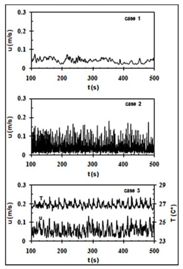
Figure 7.
Time history of velocity magnitude (for cases 1–3) and temperature (for case 3 only) at height along the line.
5.2. Power Spectral Density (PSD) Analysis
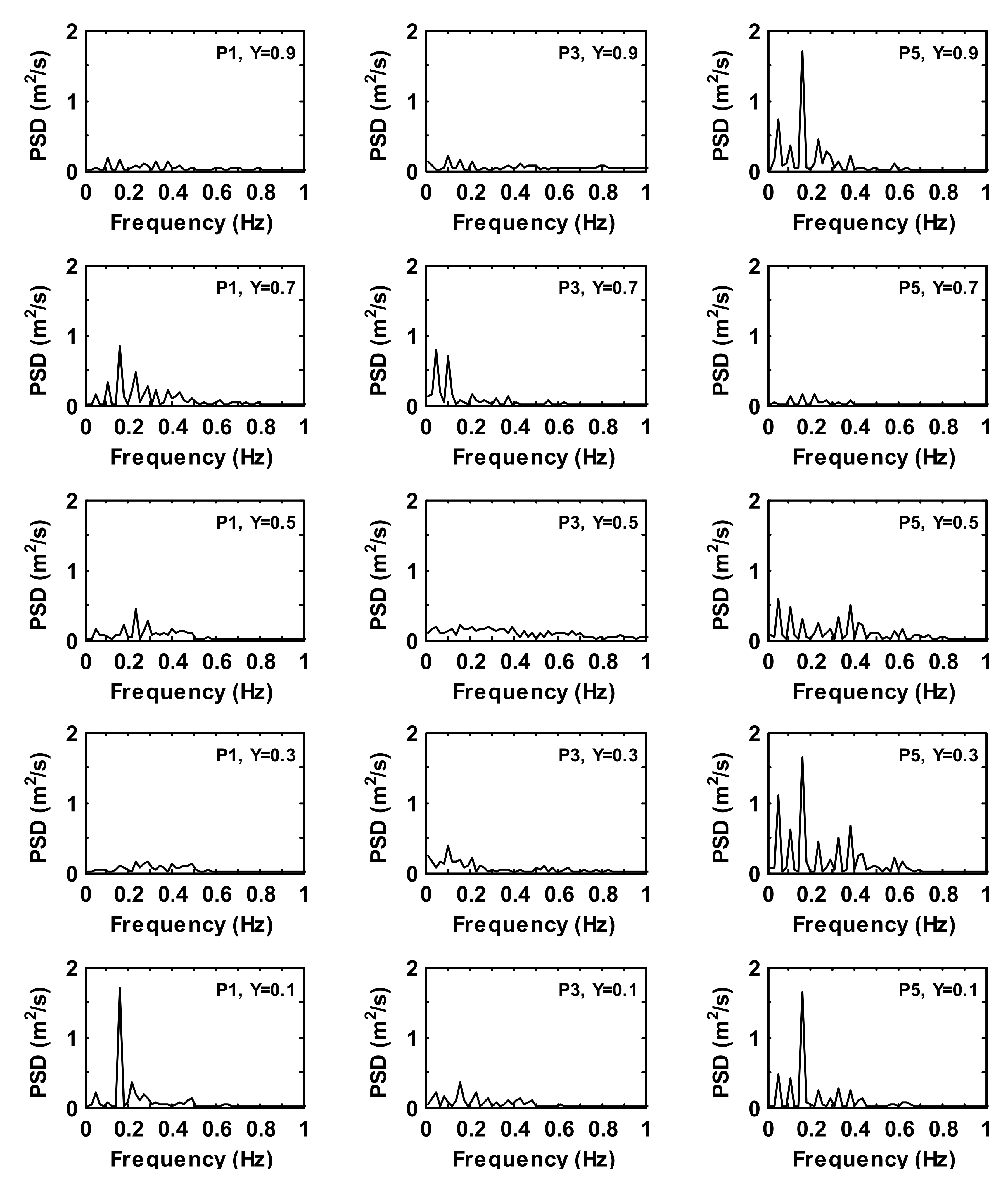
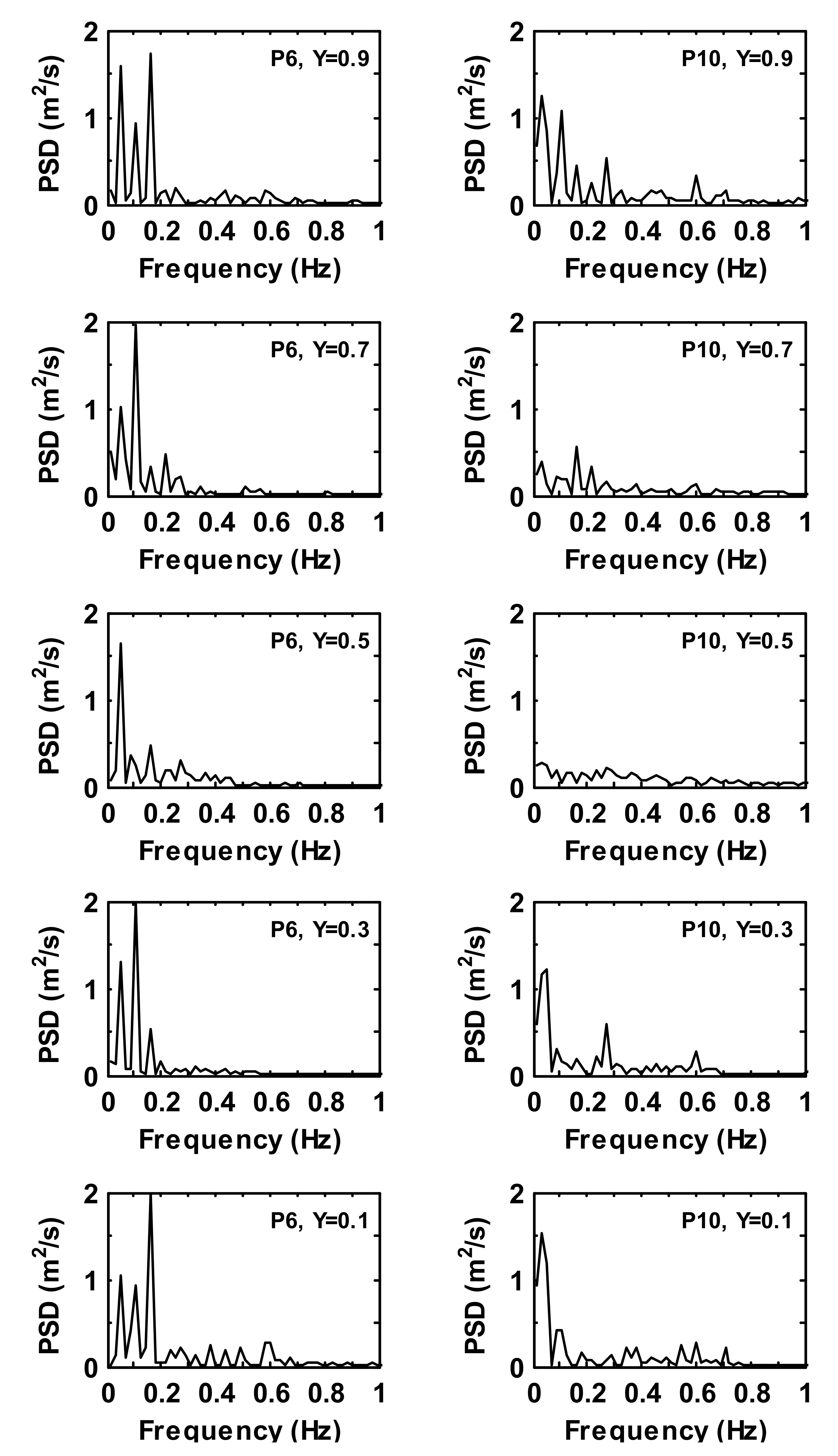
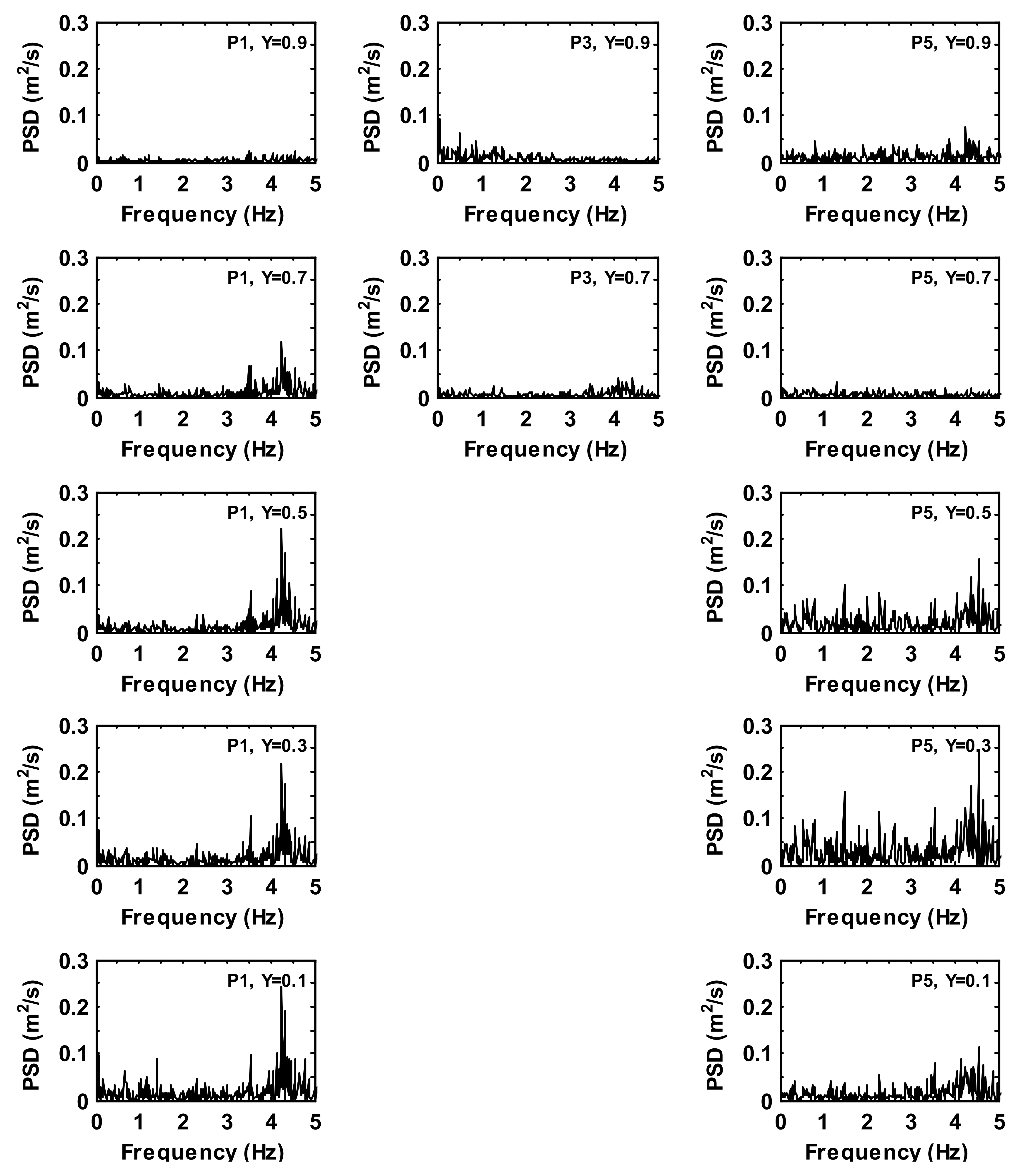
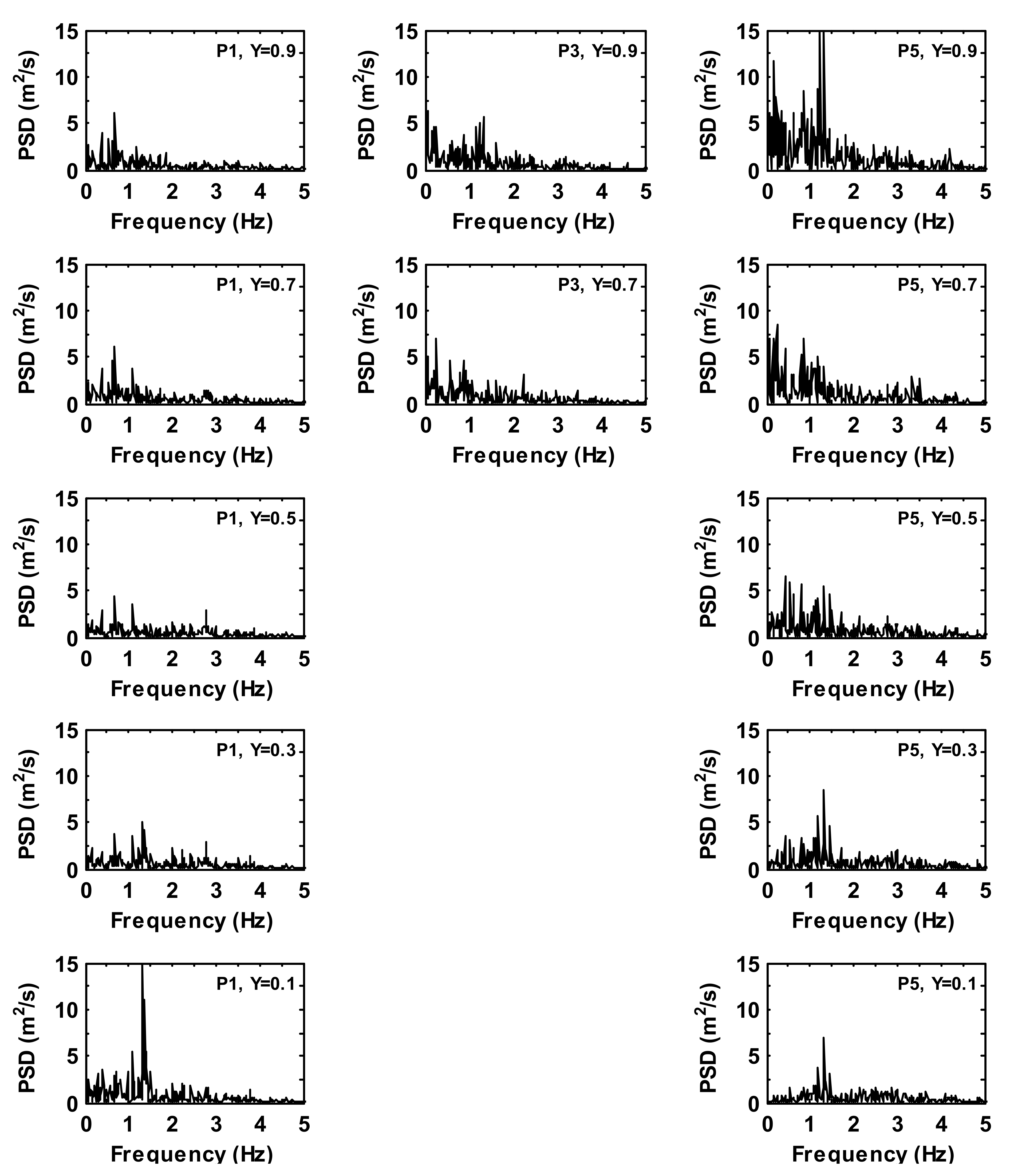
Figure 8 and Figure 9 give the power spectral density (PSD) of the velocity magnitude of the time history series at five monitoring locations for an empty domain (case 1). It can be seen that the base frequencies are found to be lower than [4] and the maximum power spectral density is about at of A single dominant frequency is found at about at at and , and at , and along the height of the location. In general, the large kinetic energy of the velocity fluctuations is found near the floor and ceiling levels at (along the back wall of the domain), and (on a spanwise plane), while the energy spectra is particularly small near the inlet opening (e.g., at and ) and at the midheight of the domain (i.e., ), consistent with the previously published work [4].

Figure 8.
Power spectra density of the time history of velocity magnitude at prescribed monitoring locations for case 1.
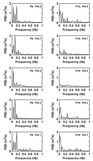
Figure 9.
Power spectra density of the time history velocity magnitude fluctuations at monitoring locations for case 1.
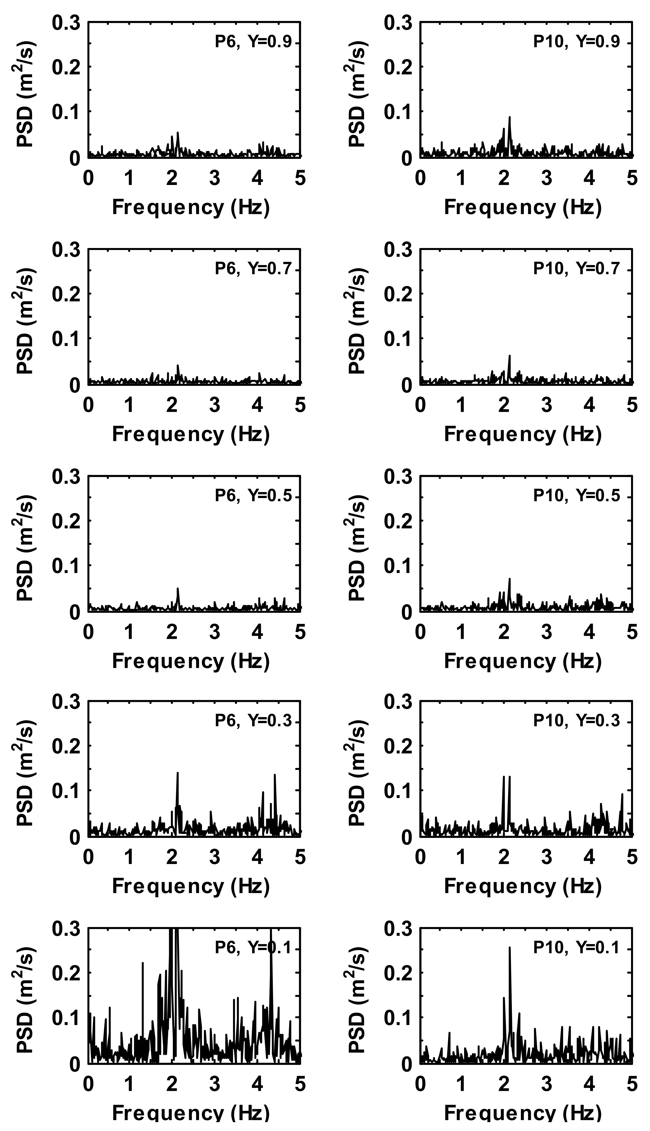
Figure 10 and Figure 11 show the power spectral density of the velocity magnitude in the time history series at five monitoring points for an unheated box (case 2). It can be seen that the base frequencies are between and . The maximum value of the power spectral density, , is observed at at of . The range of the active frequencies is higher than those in case 1, but the maximum energy of the velocity oscillations is lower. The kinetic energy of the velocity fluctuation increases with the distance between the ceiling level (i.e., ) and the monitoring locations , and . However, its energy level is relatively weak in the upper half of the domain for all the monitoring locations. The dominant frequency is clearly seen at the different magnitudes in the lower half on the mid-planes (e.g., between and for , and in a range of on a streamwise midplane, whereas it is for in a range of on a spanwise midplane). At monitoring location , due to a clockwise flow recirculation on the top of the box and an inflow ‘cold’ jet stream near the ceiling, the behavior of flow oscillations becomes irregular between level and level , where a dominant frequency is found in a range between and , respectively.

Figure 10.
Power spectra density of the time history velocity magnitude fluctuations at monitoring locations for case 2.
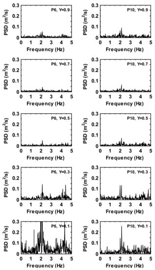
Figure 11.
Power spectra density of the time history velocity magnitude fluctuations at monitoring locations for case 2.
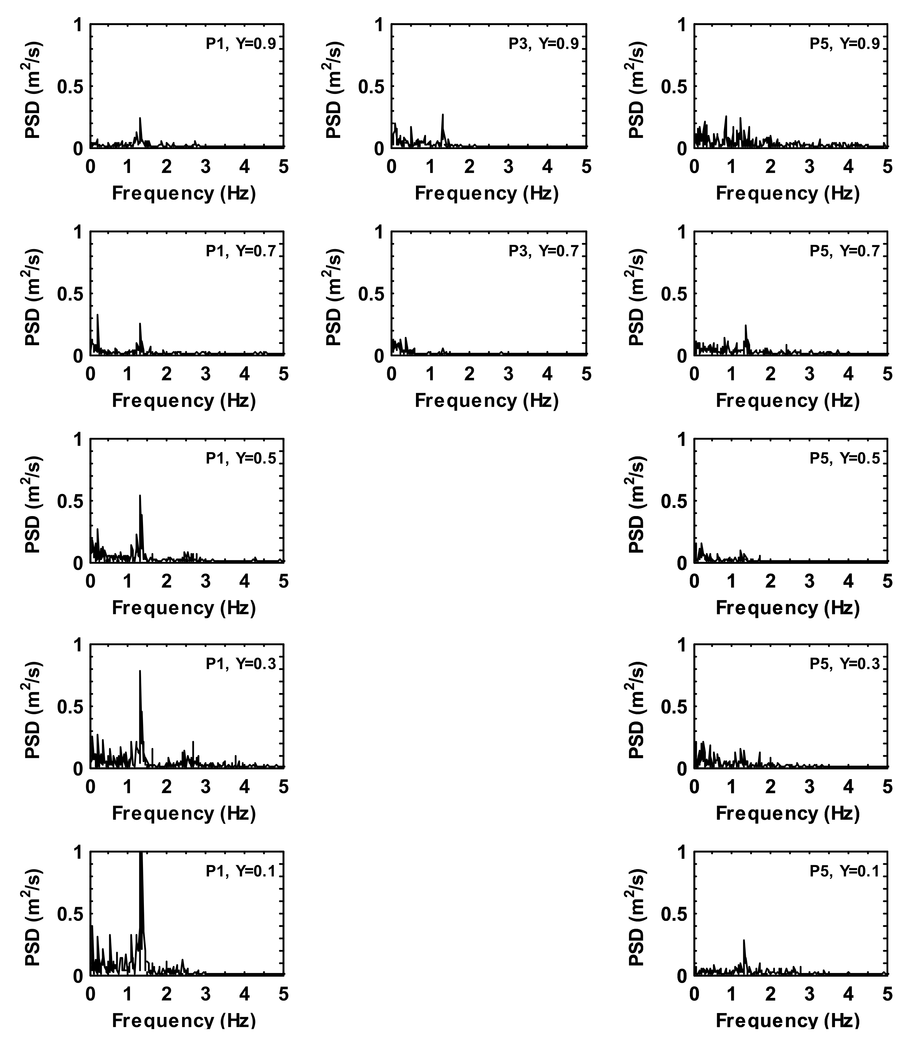
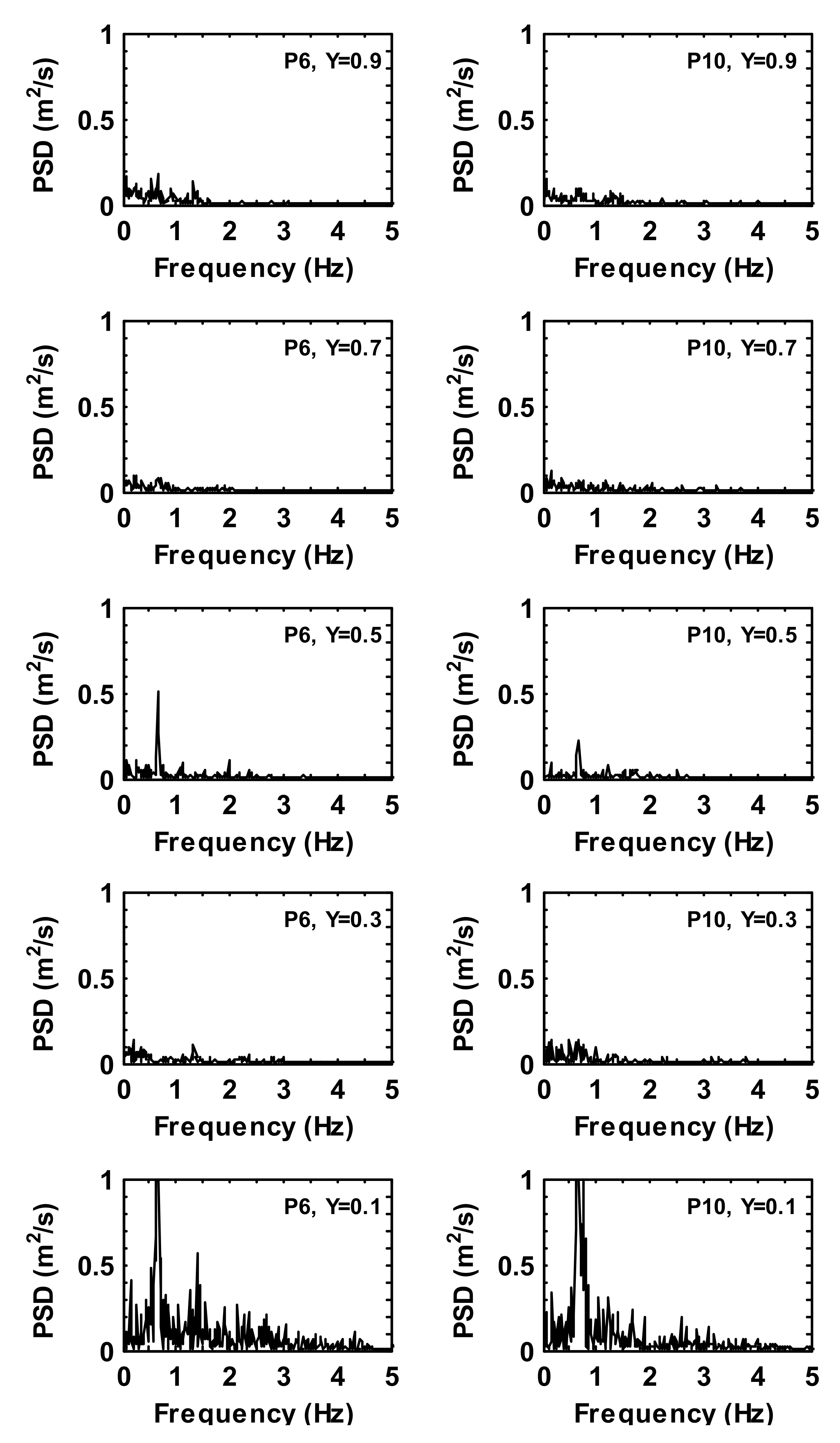
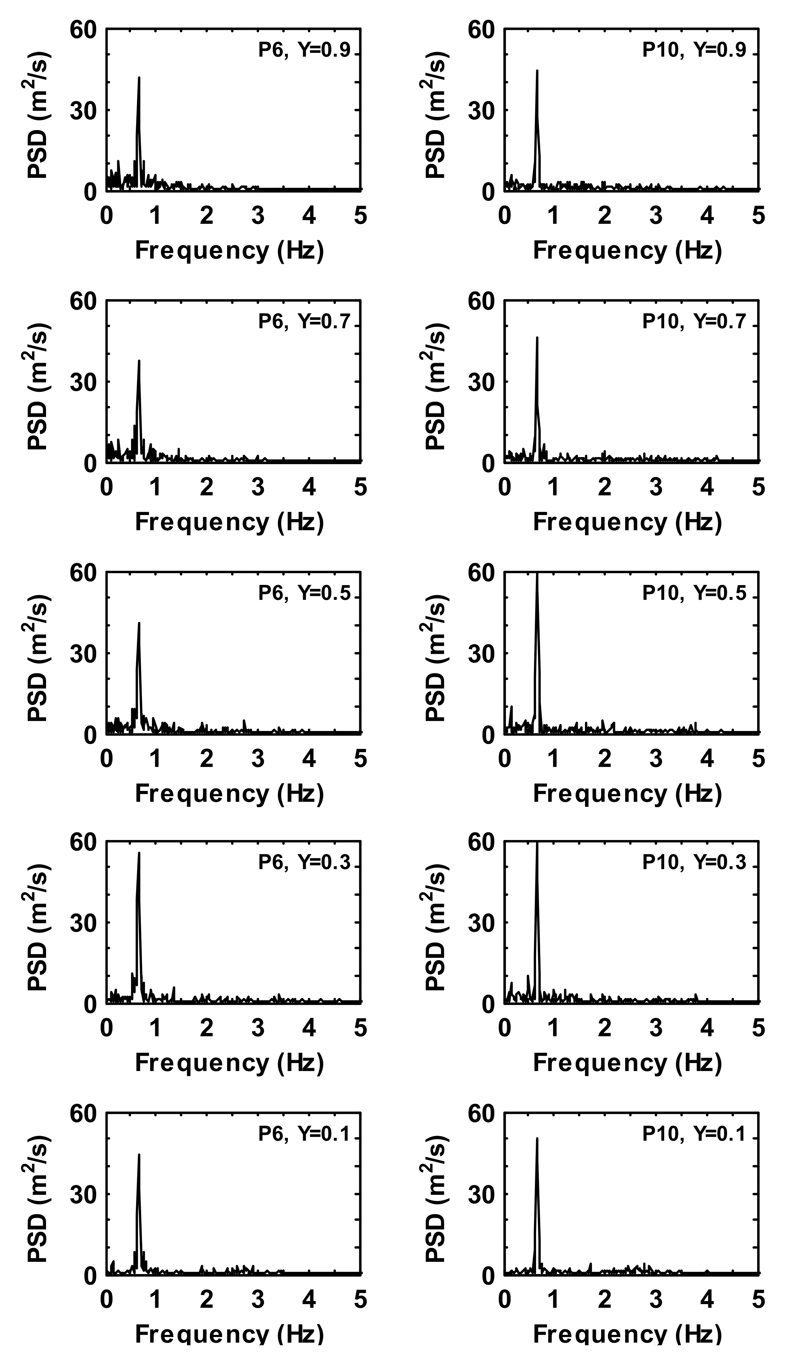
Figure 12, Figure 13, Figure 14 and Figure 15 depict the power spectral density of the velocity magnitude and temperature fluctuations in the time history series for a heated box in the fluid domain (case 3). It can be seen that the base frequencies for the velocity and temperature fluctuations are less than , although there is considerable energy difference between the velocity and temperature fluctuations. The maximum power spectral density is at of for the velocity variable, which is stronger than that of case 2, and at of for the temperature variable. The dominant frequencies found from the velocity oscillations are consistent with those of the temperature oscillations, around for and on a streamwise plane and for and on a spanwise plane. Similar to case 2, a different and higher dominant frequency is obtained at monitoring locations on a streamwise midplane compared with that of monitoring locations on a spanwise midplane. However, unlike case 2, there is no clear energy increase with the domain height for the velocity and temperature oscillations, except for the location. The highest energy of the velocity oscillation is found at the level for the three locations , and , of which at and , the power spectral density is three times stronger than that of (although the graphs only show the -axis up to . The strongest energy of the temperature fluctuation is observed at and on a spanwise plane along the domain height, two to three times stronger than the highest energy value of the other locations (as seen in Figure 14 and Figure 15, respectively). Furthermore, the dominant frequencies of case 3 are lower than that of case 2, thus representing that the heat from the box improves the flow steadiness in the fluid domain. This is probably due to the formation of the thermal plume in the fluid domain, causing it to stabilize the upper part and the sides of the heated box on a spanwise plane (see, e.g., Figure 4). Another factor could be the adiabatic wall condition used in the present study, which could decrease the flow stability in near wall regions, similar to that discussed in a previous work [9].
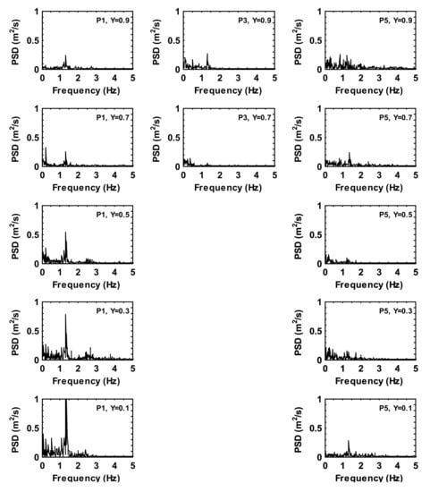
Figure 12.
Power spectra density of the time history velocity magnitude fluctuations at monitoring locations for case 3.
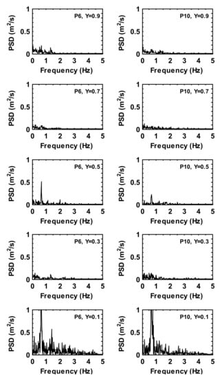
Figure 13.
Power spectra density of the time history velocity magnitude fluctuations at monitoring locations for case 3.
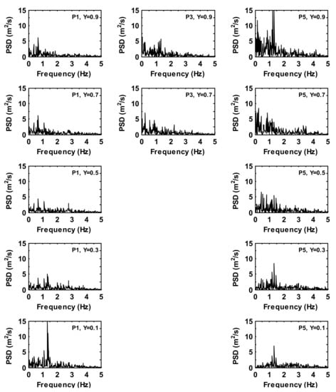
Figure 14.
Power spectra density of the time history temperature fluctuations at monitoring locations for case 3.
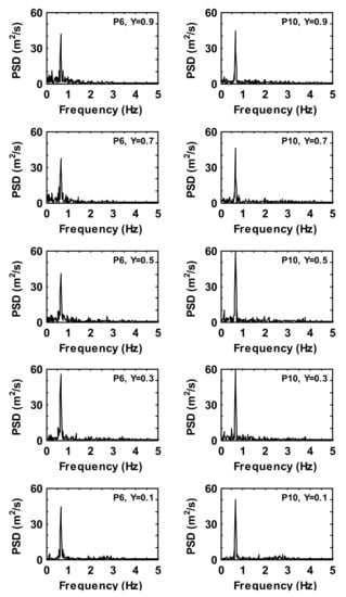
Figure 15.
Power spectra density of the time history temperature fluctuations at monitoring locations for case 3.
Figure 16 illustrates the trend of the basic frequency of the velocity fluctuations at five selected monitoring locations for all three cases. It can be seen that each case has exhibited a different frequency range, e.g., for case 1, for case 2 and for case 3. The frequency change throughout the height of the monitoring points is also found to be larger in case 3 compared with that of case 1 and case 2. In case 2, the frequency variation is almost constant along the height, except for P3, in which the variation range is the largest. At location and , the frequency is almost uniform between and for three cases. At location , the highest frequency is found at and in case 1 and case 3, respectively, while it is consistent along the height in case 2. A similar frequency distribution is seen at for case 1 and case 3, showing the lowest frequency at and the largest frequency at and .
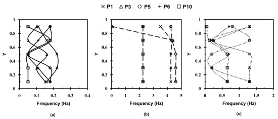
Figure 16.
Overall trends of predicted basic frequency of velocity fluctuations at five monitoring locations. (a) Case 1, (b) case 2 and (c) case 3.
6. Conclusions
A numerical investigation of unsteady flow oscillations in a 3-D ventilated model room has been conducted for three configurations from simple to moderate complex scenarios by a computational fluid dynamics approach. The computational model was carefully validated against the published data [14] for three scenarios with an increased complexity of flow and thermal features by adding a small cubic box with/without thermal load in a model room. After the validation, the model was used to investigate the development of the flow unsteadiness using the FFT technique for each scenario.
The results of forced convection flow in an empty-square domain (case 1) showed that there is no direct relation between the velocity and turbulent flow in terms of power spectral density and frequency, and each of the time history velocity oscillations are independent and random. The basic frequency of the velocity fluctuation is less than . The kinetic energy of the velocity fluctuation is relatively weak at the midheight of the domain (). Adding an unheated box in the center of the domain (case 2) induced more flow unsteadiness in the lower levels on a streamwise midplane (i.e., at and ) and at on a spanwise midplane (i.e., at and ). A dominant frequency was observed to be larger, and its energy level was weaker than that of case 1, confirming that the velocity oscillates faster in case 2. This dominant frequency depended on the orientation of the flow circulation, for example, the monitoring locations and on a streamwise midplane had shown higher dominant frequency than the locations and on a spanwise midplane. The effect of a nonheated box in the domain on the flow feature was seen on irregular oscillations in the level of of , where the strongest oscillation energy was found, possibly caused by the clockwise recirculations above the top of the box. In case 3, the frequency of velocity oscillation was decreased compared with that of case 2, and its values were consistent with the temperature at the location, although the energy of the fluctuation was much higher in temperature. Similar to case 2, the oscillation dependency on the flow orientation was seen in case 3. The maximum level of the oscillations was found at the lowest level (i.e., ) at , and for the airflow velocity and through the domain height at and (i.e., spanwise midplane) for the temperature.
Based on the three cases studied, it is found that case 3 has exhibited the highest dominant frequency in a range of 4.3–4.6 Hz, but having the lowest kinetic energy, at about 1.25 m2⁄s. For cases 1 and 2, unsteady flow oscillation phenomena are likely due to the high Grashof number and corner flow recirculation, and for case 3, it is a combination effect of a high Grashof number, corner flow recirculation and thermal instability influenced by the unsteady motion of thermal plume. Thus, it can be concluded from this study that the formation of the thermal plume from the heated box can stabilize the unsteady flow motion in the upper part to some extent. However, the sides of the heated box on a spanwise plane have played a major role in producing unsteady flow oscillations, as observed from these case studies. This finding could be useful for building designers in improving indoor air quality and energy consumption.
Author Contributions
Conceptualization, J.Y. and Y.Y.; methodology, J.Y. and Y.Y.; software, J.Y.; validation, J.Y.; for-mal analysis, J.Y.; investigation, J.Y.; resources, J.Y.; data curation, J.Y.; writing—original draft preparation, J.Y.; writing—review and editing, Y.Y.; visualization, J.Y.; supervision, Y.Y.; project administration, J.Y.; funding acquisition, J.Y. All authors have read and agreed to the published version of the manuscript.
Funding
We would like to acknowledge the partial sponsorship from Mitsubishi Electric R&D Europe MERCE-UK (E&E10-CON256, E&E11-CON256 and E&E12-CON256). The APC was partly funded by the University of the West of England, Bristol, UK.
Institutional Review Board Statement
Not applicable.
Informed Consent Statement
Not applicable.
Data Availability Statement
The data presented in this study are available on request from the corresponding author.
Acknowledgments
We wish to thank Kana Horikiri for her contribution in some data analysis and for preparing an early draft of the manuscript.
Conflicts of Interest
The authors declare no conflict of interest.
References
- Fanger, P.O.; Pedersen, C.J.K. Discomfort due to air velocities in spaces. In Proceedings of the Meeting of Commissions B1, B2, E1 of the IIR, 4, Belgrade, Yugoslavia, 4 October 1977. [Google Scholar]
- Thorshauge, J. Air-velocity fluctuations in the occupied zone of ventilated spaces. ASHRAE Trans. 1982, 2, 753–764. [Google Scholar]
- Hanzawa, H.; Melikow, A.K.; Fanger, P.O. Field measurements of characteristics of turbulent air flow in the occupied zone of ventilated spaces. In Proceedings of the CLIMA 2000 World Congress on Heating, Ventilating and Air-Conditioning, 4, Copenhagen, Denmark, 25–30 August 1985; Fanger, P.O., Ed.; VVS Kongress-VVS Messe: Copenhagen, Denmark, 1985; Volume 3 Energy Management. [Google Scholar]
- Tian, Y.S.; Karayiannis, T.G. Low turbulence natural convection in an air filled square cavity Part 2: The turbulence quantities. Heat Mass Transf. 2000, 43, 867–884. [Google Scholar] [CrossRef]
- Gebhart, B.; Mahajan, R. Chatacteristic distrubance frequency in vertical natural convection flow. Int. J. Heat Mass Transf. 1975, 18, 1143–1148. [Google Scholar] [CrossRef]
- King, K.J. Turbuleny Natural Convection in Rectanglar Air Cavities. Ph.D. Thesis, Queen Mary and Westfield College, University of London, London, UK, 1989. [Google Scholar]
- Beya, B.B.; Lili, T. Oscillatory double-diffusive mixed convection in a two-dimensional ventilated enclosure. Int. J. Heat Mass Transf. 2007, 50, 4540–4553. [Google Scholar] [CrossRef]
- Kovanen, K.; Seppane, O.; Siren, K.; Majanen, A. Turbulent air flow measurements in ventilated spaces. Environ. Int. 1989, 15, 621–626. [Google Scholar] [CrossRef]
- Henkes, R.A.W.M.; Hoogendoorn, C.J. Bifurcation to unsteady natual convection for air and water in a cavity heated from the side. In Proceedings of the 9th International Heat and Transfer Conference, 2, Jerusalem, Israel, 19–24 August 1990. [Google Scholar]
- Sinha, S.L.; Arora, R.C.; Roy, S. Numerical simulation of two-dimensional room air flow with and without buoyancy. Energy Build. 2000, 32(10), 121–129. [Google Scholar] [CrossRef]
- Stavridou, A.D.; Prinos, P.E. Unsteady CFD Simulation in a Naturally Ventilated Room with a Localized Heat Source. Procedia Environ. Sci. 2017, 38, 322–330. [Google Scholar] [CrossRef]
- Gondal, I.A.; Syed Athar, M.; Khurram, M. Role of passive design and alternative energy in building energy optimization. Indoor Built Environ. 2021, 30, 278–289. [Google Scholar] [CrossRef]
- Mesenholler, E.; Vennemann, P.; Hussong, J. Unsteady room ventilation—A review. Build. Environ. 2020, 169, 106595. [Google Scholar] [CrossRef]
- Wang, M.; Chen, Q. Assessment of various turbulence models for transitional flows in enclosed environment (RP-1271). HVAC Res. 2009, 15, 1099–1119. [Google Scholar] [CrossRef]
- Horikiri, K.; Yao, Y.F.; Yao, J. Numerical study of unsteady flow phenomena in a ventilated room. Comput. Therm. Sci. 2012, 4, 317–333. [Google Scholar] [CrossRef]
- Zuo, W.; Chen, Q. Real-time or faster-than-real-time simulation of airflow in buildings. Indoor Air 2009, 19, 33–44. [Google Scholar] [CrossRef] [PubMed] [Green Version]
- Horikiri, K.; Yao, Y.F.; Yao, J. Modelling conjugate flow and heat transfer in a ventilated room for indoor thermal comfort assessment. Build. Envrion. 2014, 77, 135–147. [Google Scholar] [CrossRef] [Green Version]
- Patankar, S.V.; Spalding, D.B. A calculation procedure for heat, mass and momentum transfer in three-dimensional parabolic flow. Int. J. Heat Mass Transf. 1972, 15, 1787–1806. [Google Scholar] [CrossRef]
- Cooley, J.W.; Tukey, J.W. An Algorithm for the Machine Calculation of Complex Fourier Series. Math. Comput. 1965, 19, 297–301. [Google Scholar] [CrossRef]
- Smith, S.W. Digital Signal Processing, A Practical Guide for Engineers and Scientists; Elsevier: Amsterdam, The Netherlands, 2002. [Google Scholar] [CrossRef]
- Chen, Q.; Srebric, J. How to Verify, Validate, and Report Indoors Environment Modeling CFD Analyses; ASHRAE TC 4.10; Indoor Environmental Modeling; ASHRAE: Atlanta, GA, USA, 2001. [Google Scholar]


Publisher’s Note: MDPI stays neutral with regard to jurisdictional claims in published maps and institutional affiliations. |
© 2022 by the authors. Licensee MDPI, Basel, Switzerland. This article is an open access article distributed under the terms and conditions of the Creative Commons Attribution (CC BY) license (https://creativecommons.org/licenses/by/4.0/).