The Momentum Conserving Scheme for Two-Layer Shallow Flows

Abstract

This paper confronts the numerical simulation of steady flows of fluid layers through channels of varying bed and width. The fluid consists of two immiscible fluid layers with constant density, and it is assumed to be of a one-dimensional shallow flow. The governing equation is a coupled system of two-layer shallow water models. In this paper, we apply a direct extension of the momentum conserving scheme previously used for solving the one layer shallow water equations. Computations of various steady-state solutions are used to demonstrate the performance of the proposed numerical scheme. Under the influence of a given flow rate, the numerical steady interface is generated in a channel topography with a hump. The results obtained confirm the analytic steady interface of the two-layer rigid-lid model. Furthermore, the same scheme was used with an additional artificial damping to simulate the maximal exchange flow in channels of varying width. The numerical steady interface agreed well with the analytical steady solutions.

1. Introduction

The presence of internal waves in Indonesian waters such as the Lombok Strait and the Andaman Sea inspired this research. The internal waves in the Lombok Strait form when a layer of warm low-salinity water from the Pacific Ocean enters the strait and flows into the Indian Ocean as part of the Indonesian throughflow (ITF); the complex bathymetry of the strait with a sill also contributes to internal wave generation in Lombok Strait. These internal waves, once generated, travel through the strait; after leaving the strait’s mouth, the wave propagates radially across the ocean, to the north of the Flores Sea, and to the south of the Indian Ocean.

In order to construct a numerical model for simulating the generation and propagation of internal waves in natural straits, we must begin with a simpler numerical model that captures the most important behavior of exchange flows through channels connecting two basins with different hydrological characteristics, such as the Lombok Strait. Several researchers [1,2,3] and many others discuss the generation and propagation of internal waves in the Strait of Gibraltar. They adopted a one-dimensional two-layer shallow flow model, which can be applied to channels of varying topographies and widths, to model the influence of external flows in the strait. This one-dimensional approach is considered to be quite feasible for modelling the internal hydraulics of the strait and its effect on exchange flows [3,4,5]. While internal wave propagation in the radial direction across the ocean requires a higher dimensional approach (two-dimension or even three-dimension). Inspired by their research, in this article, we will focus on developing a numerical scheme for a one-dimensional two-layer shallow flow model as well as testing the ability of the numerical scheme to simulate the steady interface of the two-layer fluid flows.

The goal of this research study is to investigate the dynamics of flow through a one-dimensional channel connecting two reservoirs. Our method employs numerical simulation of a steady interface in a channel with varying bed and width. In this paper, we present a numerical model capable of simulating steady interfaces in a variety of situations. In contrast to the one-layer shallow water equation, the two-layer shallow water equation model is not always hyperbolic [1,6,7,8,9]. This presents its own challenges for the proposed numerical scheme. So far, the majority of numerical schemes that have been developed are associated with the finite volume or the finite difference methods. A numerical scheme based on a Riemann solver is proposed and developed by [3,9]. A finite difference scheme for solving the two-layer rigid-lid model is developed in [1], whereas a phase resolving numerical model is described in [2,5]. References [2,5] developed a numerical model capable of describing dispersive waves. In this article, we will develop a numerical scheme for solving the two-layer shallow water equations. The scheme is an extension of the momentum conserving staggered-grid scheme (MCS) for the one-layer shallow water equations [10] (see also [11]). It turns out that the newly developed scheme can be applied directly to solve two-layer shallow water models. The scheme is then validated by simulating different steady two-layer flows, including those with hydraulic jumps. We will simulate the formation of a steady interface in the channel due to the presence of a bottom sill. The numerical scheme will be validated further by simulating the maximal exchange flow in a channel of varying width.

Thus, the outline of this paper is as follows: discussions about the two-layer shallow water models followed with some review about the steady hydraulics of two-layer rigid-lid models are presented in Section 2; formulations of the momentum conserving schemes for solving the two-layer shallow water models are presented in Section 3; and various steady-state problems are simulated in Section 4 and Section 5 to validate the proposed scheme. Finally, the conclusion is provided in Section 6.

2. Mathematical Model

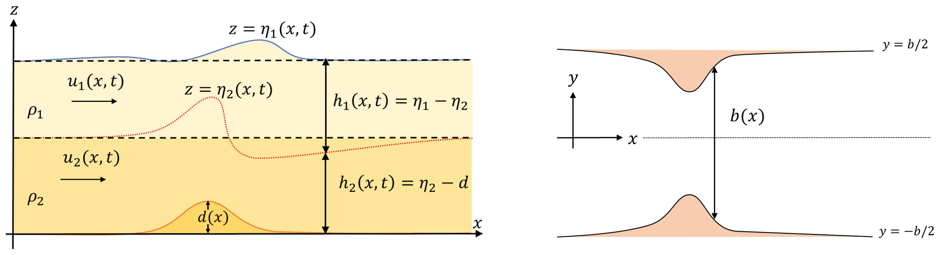
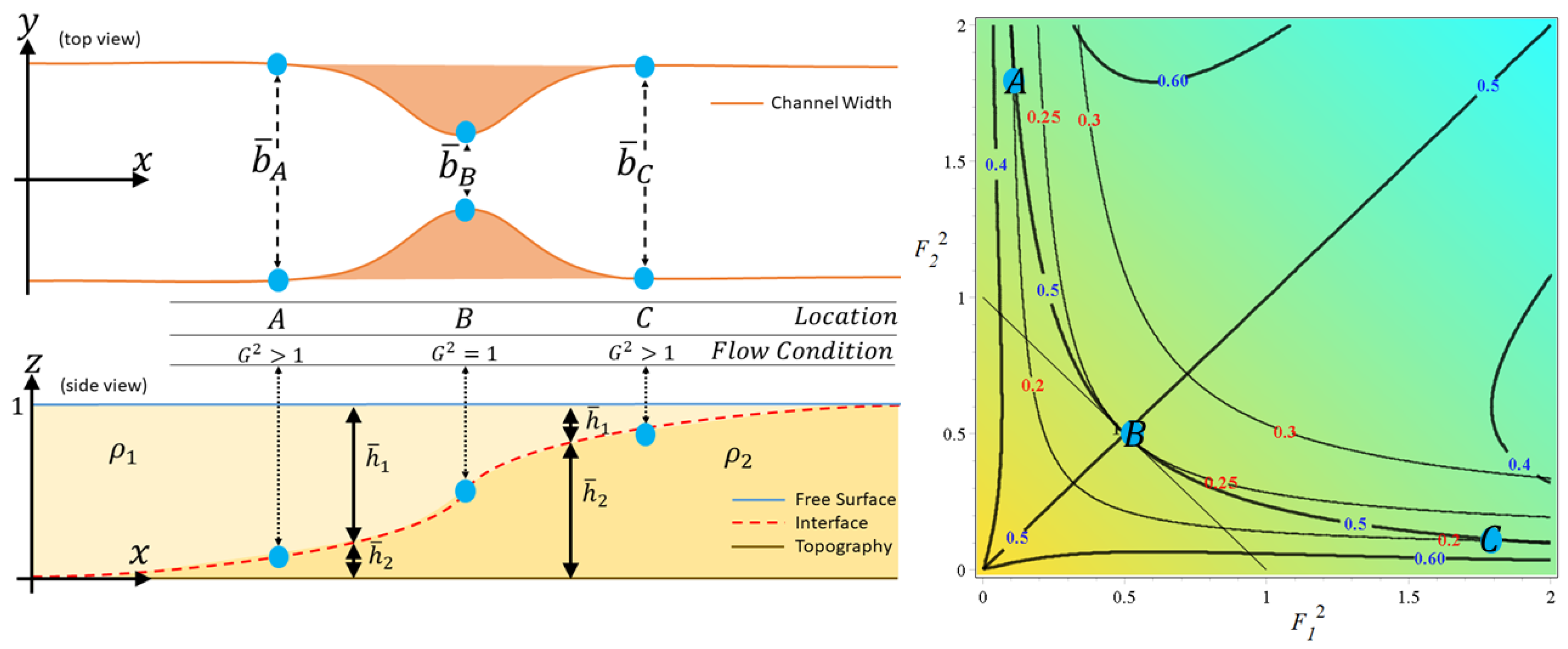
We begin with a discussion on the governing equations for the two-layer fluid in a one-dimensional channel. Here, the channel cross-section is assumed to be rectangular, with varying bed, and varying width. Assume that the fluid consists of two immiscible layers of different densities. The upper fluid has density ${\rho }_1$, and the lower fluid has density ${\rho }_2$, with ${\rho }_2>{\rho }_1$. Let $z={\eta }_1(x,t)$ represent free surface deformation, $z={\eta }_2(x,t)$ denotes the interface between two fluids, and $z=d\left(x\right)$ denots the channel bottom topography, as shown in Figure 1. Under this setting, the thickness of the upper and lower layers is $h_1={\eta }_1-{\eta }_2$ and $h_2={\eta }_2-d$, respectively. We denote $H_0$ as the reference height, where $H_0=h_1+h_2+d$. We employ a one-dimensional approach, which requires us to assume that the flow is uniform across the channel cross section. Moreover, the channel under consideration is symmetrical about the x-axis, with channel bed $d\left(x\right)$ and width $b\left(x\right)$ assumed to be slowly varying. The fluid particle velocities in the upper and lower layers is denoted as $u_1(x,t)$ and $u_2(x,t)$, respectively. Let $A_i(x,t)$ represent the cross-sectional area of fluid in each layer, whereas $Q_i(x,t)=A_i(x,t)u_i(x,t)$ denotes the discharge.

We restrict our discussion to rectangular channels, so the cross-section area is simply $A_i(x,t)=h_i(x,t)b\left(x\right)$, with $b\left(x\right)$ being the channel width. According to [7,12,13], the governing equations of the two-layer flows under hydrostatic pressure is given by the following.

$$\begin{array}{ccc}& & \frac{\partial A_1}{\partial t}+\frac{\partial Q_1}{\partial x}=0,\hfill \end{array}$$

(1)

$$\begin{array}{ccc}& & \frac{\partial u_1}{\partial t}+u_1\frac{\partial u_1}{\partial x}+g\frac{\partial {\eta }_1}{\partial x}=0.\hfill \end{array}$$

(2)

$$\begin{array}{ccc}& & \frac{\partial A_2}{\partial t}+\frac{\partial Q_2}{\partial x}=0,\hfill \end{array}$$

(3)

$$\begin{array}{ccc}& & \frac{\partial u_2}{\partial t}+u_2\frac{\partial u_2}{\partial x}+g\frac{{\rho }_1}{{\rho }_2}\frac{\partial {\eta }_1}{\partial x}+g\left(1-\frac{{\rho }_1}{{\rho }_2}\right)\frac{\partial {\eta }_2}{\partial x}=0.\hfill \end{array}$$

(4)

Equations (1) and (3) are mass conservation for the upper and lower layer, respectively. Equations (2) and (4) are the momentum balances for each layer. In this paper, we will propose a numerical scheme for solving the two-layer model (1)–(4). However, we first provide a brief review here on the formulation of steady two-layer solutions.

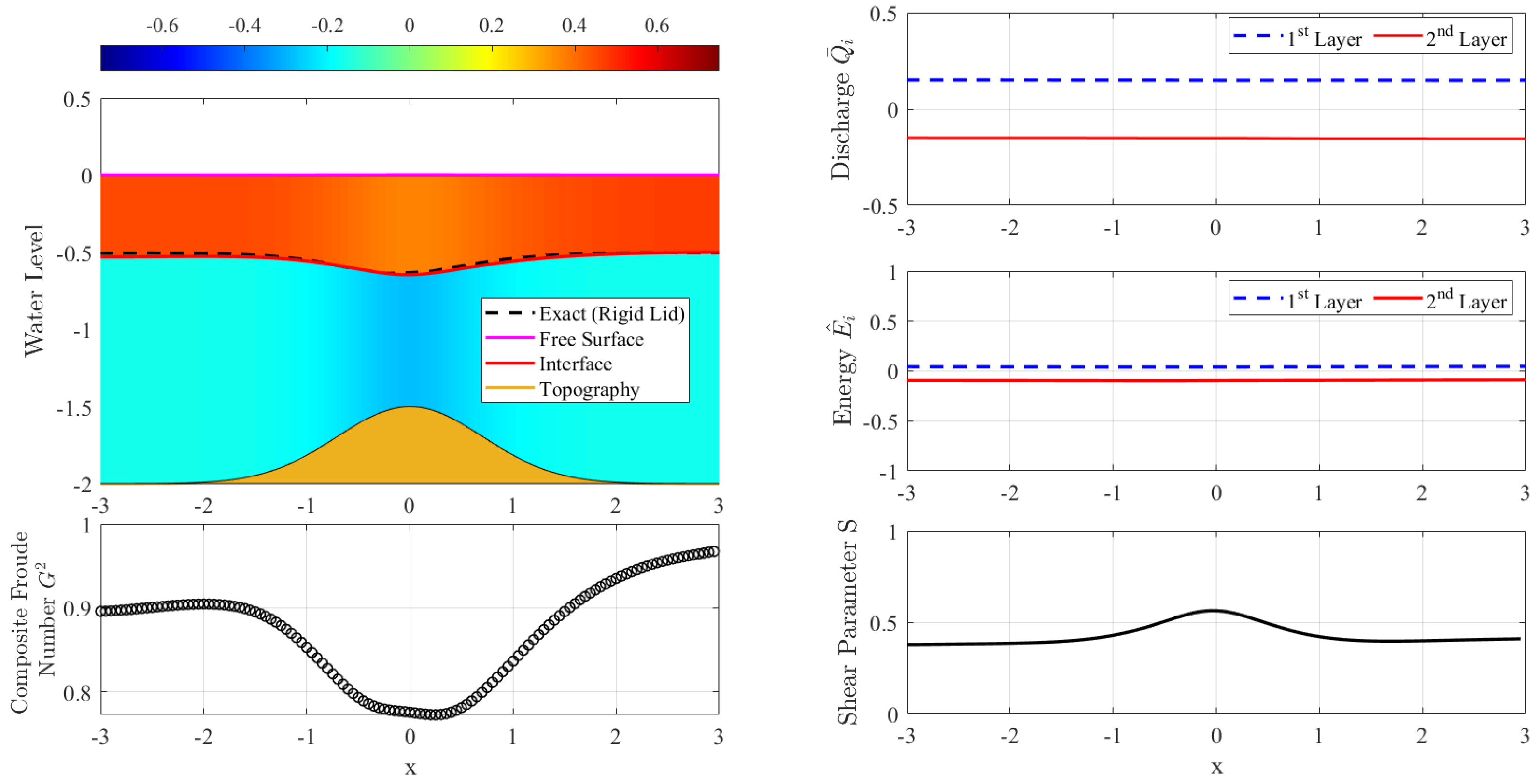
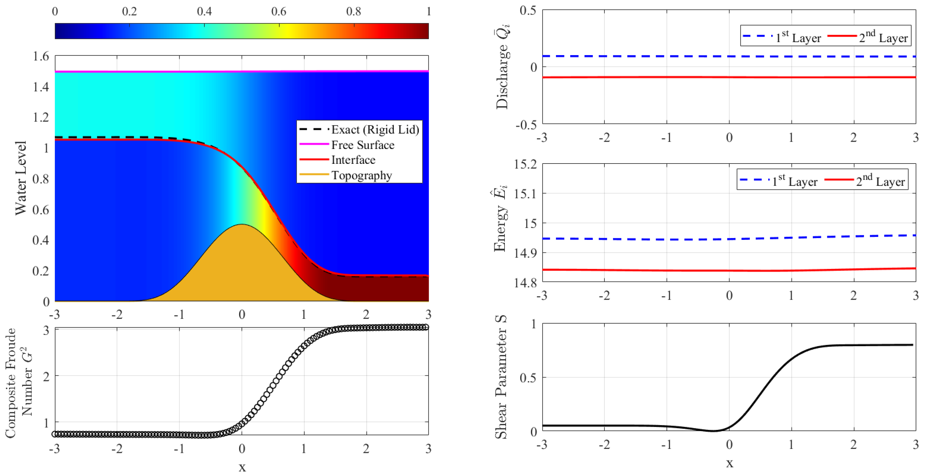
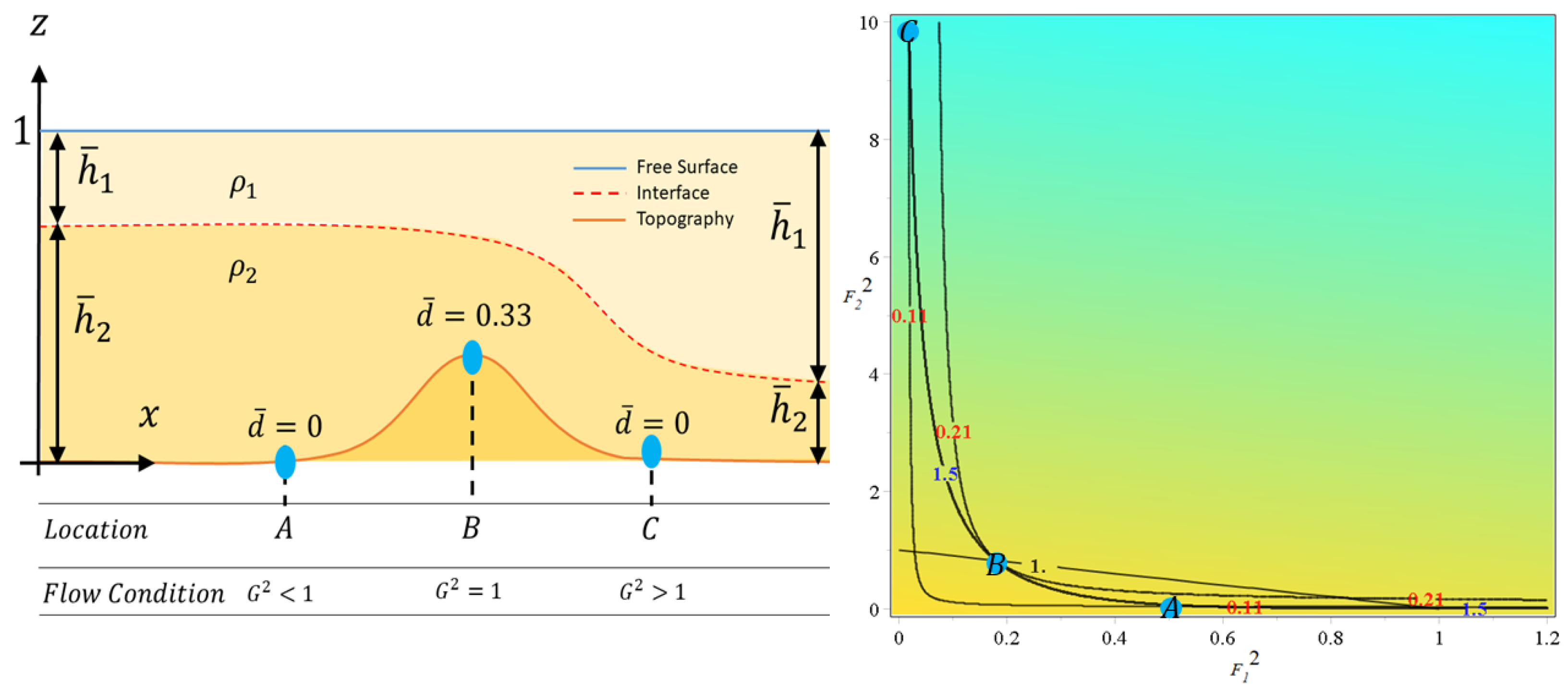
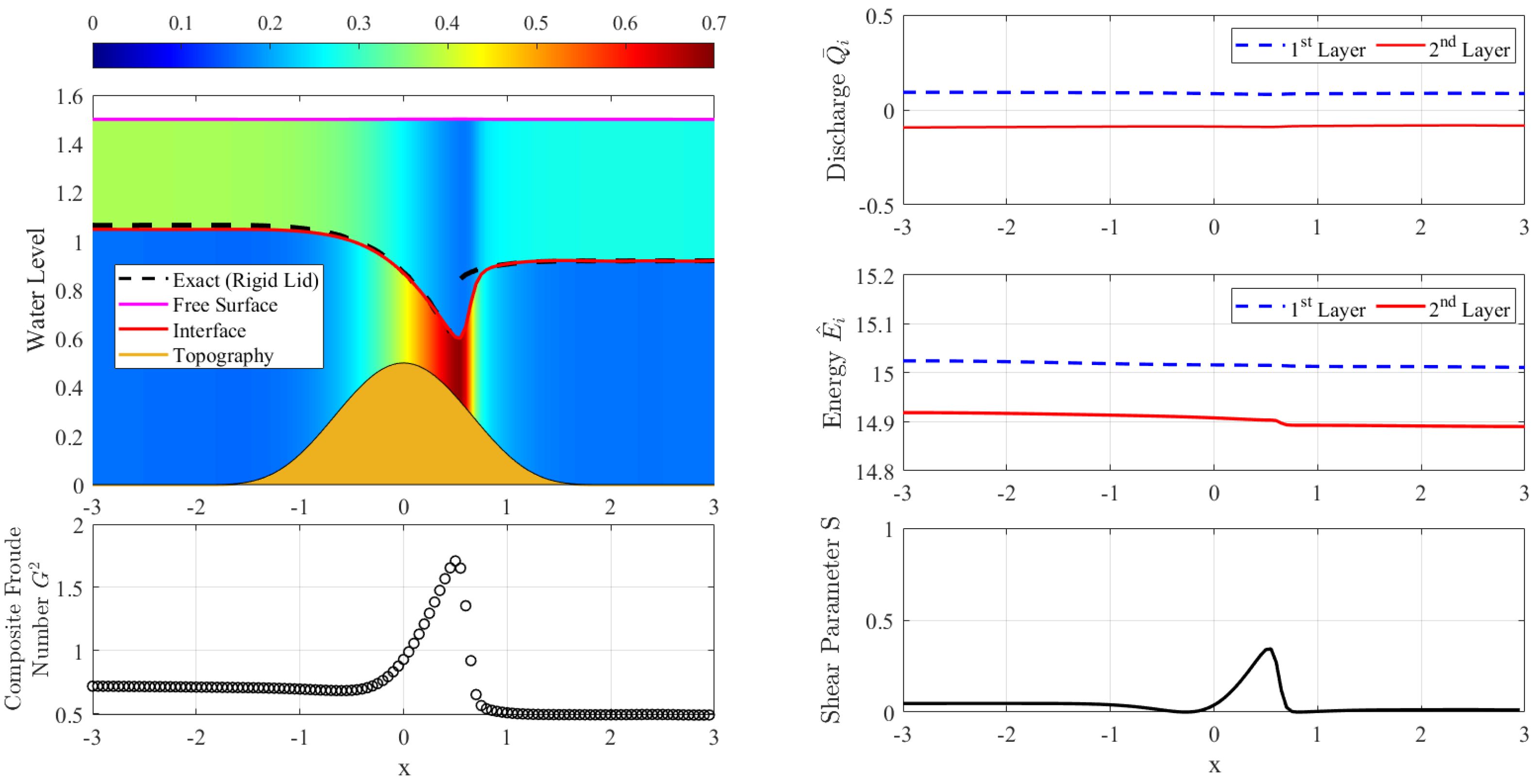
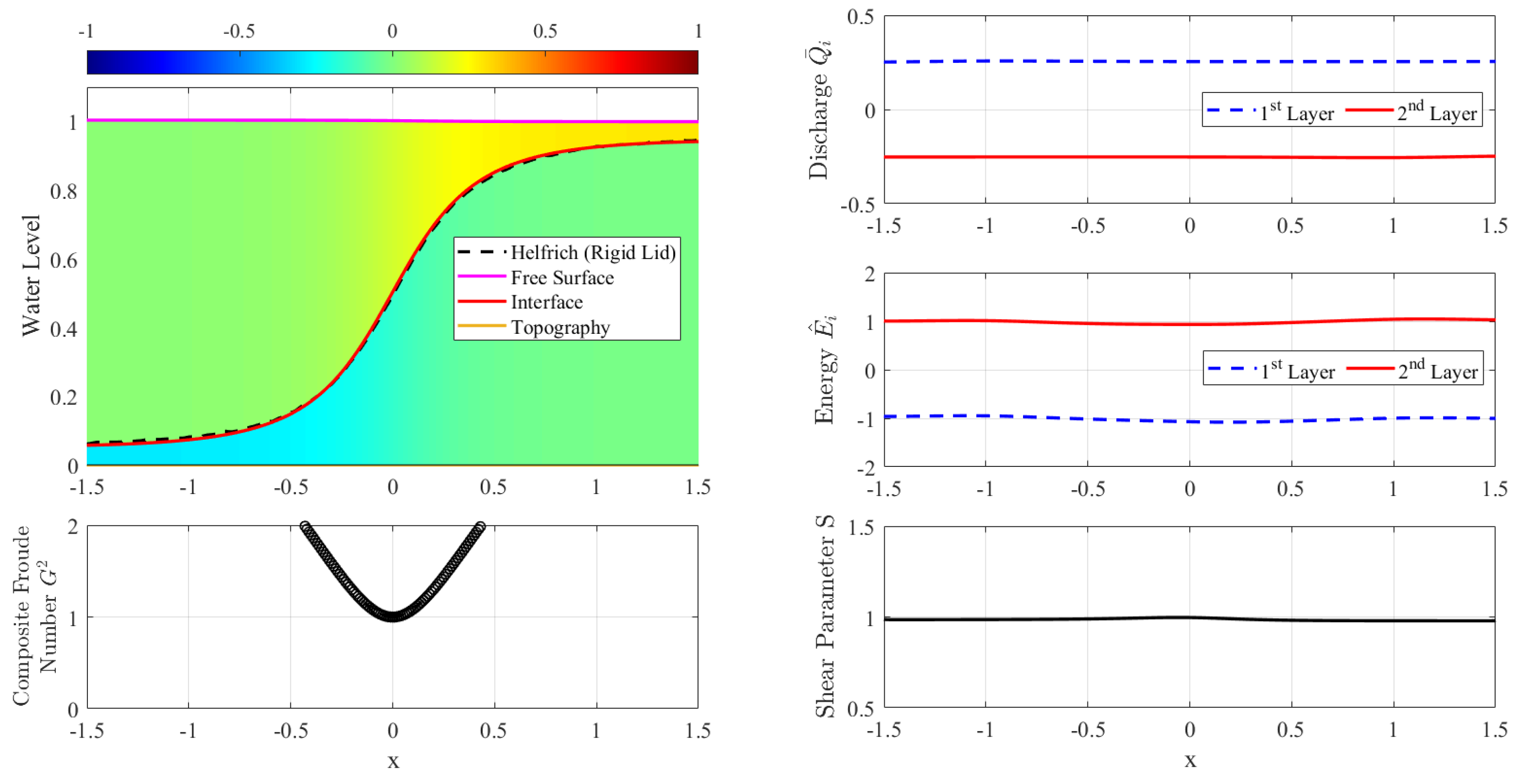
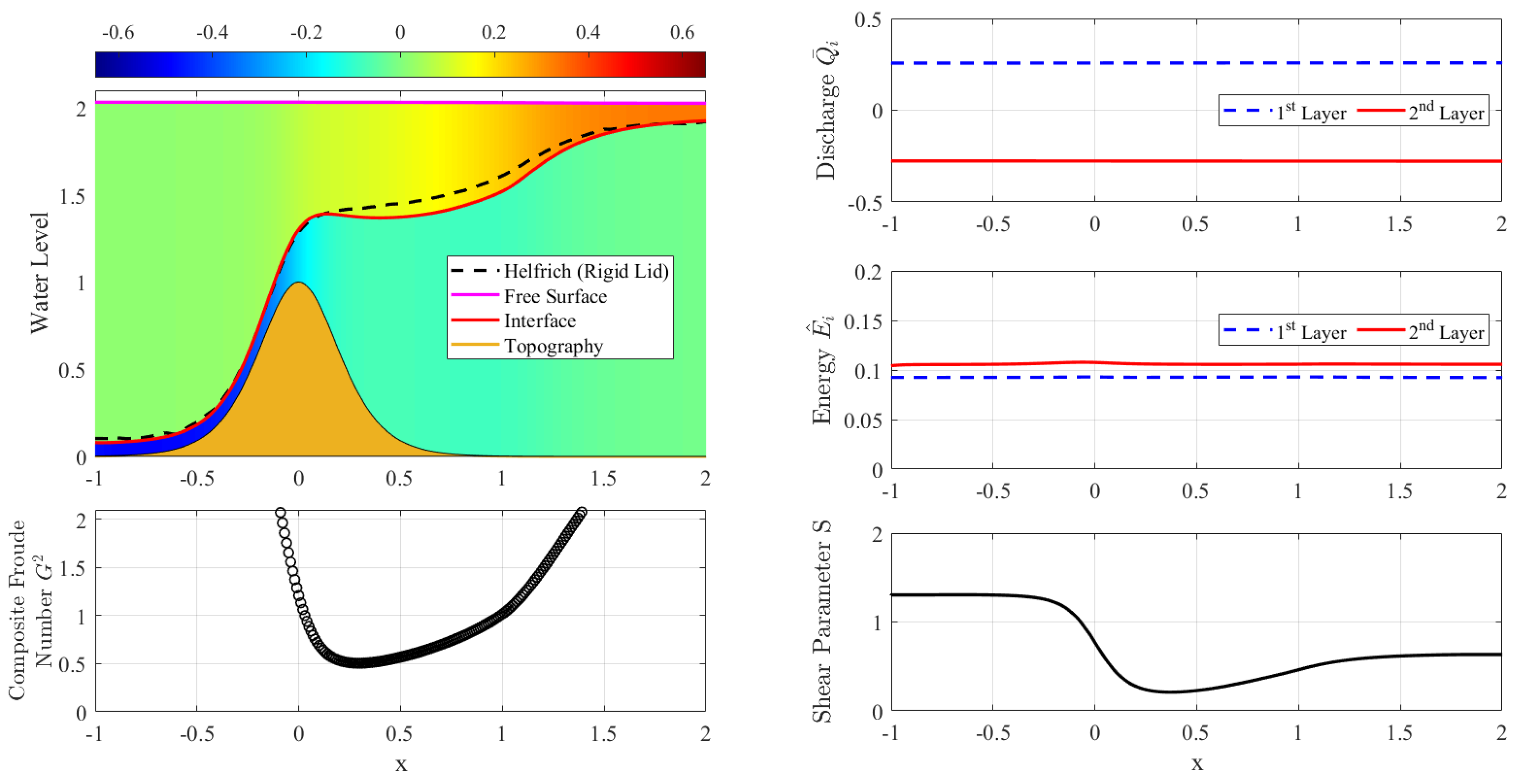
2.1. Steady Two-Layer Solutions

Farmer and Armi [4], Armi [6] conducted an in-depth study of the steady-flow of the two-layer rigid-lid model. The results of their study have been widely used to validate numerical schemes [1,3,7,9]. In the following description, we will present a brief review of the Armi Farmer steady solution, which will be used to validate our numerical scheme.

In the steady situation, mass conservation (1) and (3) reduces to ${\widehat{Q}}_1=A_{1}b$ and ${\widehat{Q}}_2=A_{2}b$, respectively, whereas the momentum Equations (2) and (4) lead to the specific energy for each layer as follows.

$$\begin{array}{ccc}& & {\widehat{E}}_1=\frac{1}{2}{\rho }_1{u}_1^2+g{\rho }_1(h_1+h_2+d),\hfill \end{array}$$

(5)

$$\begin{array}{ccc}& & {\widehat{E}}_2=\frac{1}{2}{\rho }_2{u}_2^2+g{\rho }_2(h_2+d)+g{\rho }_1{h}_1.\hfill \end{array}$$

(6)

In the above description, notations with hats represent steady variables. By subtracting the energy equations in (5) and (6) after dividing with $g^{\prime }{\rho }_2{H}_0$ and after some algebra, one obtains the following:

$$\begin{array}{ccc}& & \frac{{\widehat{E}}_1-{\widehat{E}}_2}{g^{\prime }{\rho }_2{H}_0}=\frac{1}{2g^{\prime }{H}_0}\left(r{u}_1^2-u_2^2\right)-\frac{h_2+d}{H_0},\hfill \end{array}$$

(7)

where $r=\frac{{\rho }_1}{{\rho }_2}$ and $g^{\prime }\equiv g(1-r)$, which represents reduced gravity. The energy difference (7) is also known as the Bernoulli equation [4].

Let the Froude number for each layer be denoted as follows.

$$\begin{array}{ccc}& & F_i^2=\frac{u_i^2}{g^{\prime }{h}_i}=\frac{Q_i^2}{g^{\prime }{b}^2{h}_i^3},i=1,2.\hfill \end{array}$$

(8)

As discussed in [6], the two-layer model (1)–(4) reaches a critical condition when $G^2=1$ in which $G^2$ the composite Froude number for two-layer flows with free surface is given by the following.

$$\begin{array}{ccc}& & G^2\equiv F_1^2+F_2^2-(1-r)F_1^2{F}_2^2.\hfill \end{array}$$

For layers with $r\approx 1$, the composite Froude number can be approximated to $G^2\approx F_1^2+F_2^2$, and the criticality condition becomes the following.

$$\begin{array}{ccc}& & F_1^2+F_2^2=1.\hfill \end{array}$$

(9)

If $G^2<1$, the flow is called subcritical, whereas if $G^2>1$ the flow is called supercritical. When $G^2=1$, the flow is said to be critical, and its location is called a control.

Unlike the one-layer shallow water equation which is always hyperbolic, the two-layer Equations (1)–(4) are not always hyperbolic. The hyperbolic property of the two-layer equations depends on a parameter called the shear parameter,

$$S\equiv \frac{{(u_1-u_2)}^2}{g^{\prime }(h_2+h_1)}.$$

(10)

The model will be hyperbolic if $S<1$, in this case, the characteristic velocities are real numbers. However, if $S>1$ the characteristic velocities becomes complex numbers, and the model changes from hyperbolic to elliptic [14].

The stability condition (10) is related to the Kelvin–Helmholtz instability. If this instability occurs, this means that the two previously immiscible fluids begin to mix. The energy will be reduced as a result of this mixing process. Numerically, this instability will cause spurious error in the calculation, causing the scheme to become unstable [1,8,9,12]. To control this instability, some dissipation must be added to the model; in this study, the artificial damping terms $\nu {\partial }_{xx}{u}_1$ and $\nu {\partial }_{xx}{u}_2$ is added to the momentum Equations (2) and (4), respectively.

The most common approximation used is the rigid-lid approximation. In this approximation, free surface deformation is neglected or ${\eta }_1$ is constant over time. When dealing with a rigid lid, the following relation must be added:

$$h_1+h_2+d=H_0,$$

(11)

with $H_0$ the reference height.

2.2. Formulation Using Normalized Variables

Furthermore, we define the following non-dimensional variables of free surface, interface, fluid thicknesses, channel width, bottom elevation, and discharges:

$$\begin{array}{ccc}& & {\overline{\eta }}_i=\frac{{\eta }_i}{H_0},{\overline{h}}_i=\frac{h_i}{H_0},\overline{b}=\frac{b}{b_0},\overline{d}=\frac{d}{H_0},{\overline{Q}}_i^2=\frac{Q_i^2}{g^{\prime }{b}^2{H}_0^3},i=1,2,\hfill \end{array}$$

(12)

with $b_0$ denoting the reference width. The dimensionless variables are denoted with bars, whereas the physical variables do not have bars. From the Froude number formula (8), we have the following useful relationship.

$${\overline{h}}_i={\left(\frac{{\overline{Q}}_i}{\overline{b}}\right)}^{2/3}{F}_i^{-2/3},i=1,2.$$

(13)

By using the relation (13), we can rewrite the rigid-lid Equation (11) in terms of Froude number as follows.

$$\begin{array}{ccc}& & {\left(\frac{{\overline{Q}}_1}{\overline{b}}\right)}^{2/3}{F}_1^{-2/3}+{\left(\frac{{\overline{Q}}_2}{\overline{b}}\right)}^{2/3}{F}_2^{-2/3}+\overline{d}=1,\hfill \end{array}$$

(14)

$$\begin{array}{ccc}& & {\overline{Q}}_r^{2/3}{F}_1^{-2/3}+F_2^{-2/3}={\left(\frac{{\overline{Q}}_2}{\overline{b}{(1-\overline{d})}^{3/2}}\right)}^{-2/3}.\hfill \end{array}$$

(15)

Equation (15) is called the rigid-lid curve, with $\frac{{\overline{Q}}_2}{\overline{b}{(1-\overline{d})}^{3/2}}$ being the volume flow rate.

Under the rigid-lid assumption, we have $-\overline{h_2}-\overline{d}={\overline{h}}_1-1$, so the Bernoulli Equation (7) can be rewritten as follows.

$$\begin{array}{ccc}& & \mathsf{\Delta }\widehat{E}\equiv \frac{{\widehat{E}}_1-{\widehat{E}}_2}{g^{\prime }{\rho }_2{H}_0}+1=\frac{1}{2}\left(r{\overline{h}}_1{F}_1^2-{\overline{h}}_2{F}_2^2\right)+{\overline{h}}_1.\hfill \end{array}$$

(16)

If the channel has constant width $\overline{b}=1$, the formula (16) can be written in terms of the Froude numbers and discharge ratio ${\overline{Q}}_r=|{\overline{Q}}_1/{\overline{Q}}_2|$ as follows:

$$\begin{array}{ccc}& & F_2^2={\overline{Q}}_r{\left(F_1^{-2/3}(F_1^2+2)-2\mathsf{\Delta }\overline{E}\right)}^{3/2}.\hfill \end{array}$$

(17)

where $\mathsf{\Delta }\overline{E}={\overline{Q}}_1^{-2/3}\mathsf{\Delta }\widehat{E}$.

Similarly to the one-layer shallow water model where steady hydraulics can be described as a trajectory of the energy curve, the steady interface of the two-layer model (assuming existence is guaranteed) can be described as a trajectory on the energy difference curve (17). This aspect will be discussed in detail by using specific examples in Section 4 and Section 5.

3. Numerical Model

In this section, we discuss the numerical scheme for solving the two-layer model (1)–(4). The scheme is based on the momentum conserving scheme for one-layer shallow water flows originally proposed by [15]. The scheme can be used to solve problems with rapidly varying flows, such as those involving hydraulic jumps and bores. This scheme has been implemented and extended to various shallow water flow problems, such as in [10,16,17] where it was referred to as the MCS scheme, an abbreviation for the momentum conserving staggered-grid scheme. The extension of the MCS scheme to the two-layer model has been successfully used for the study of internal waves in [18]. In this article, the scheme, which is limited to the hydrostatic model, will be used for discussion with a focus on simulating various steady flows in a channel with varying bed and width. The formulation of the MCS scheme for the two-layer hydrostatic model (1)–(4) will be described below.

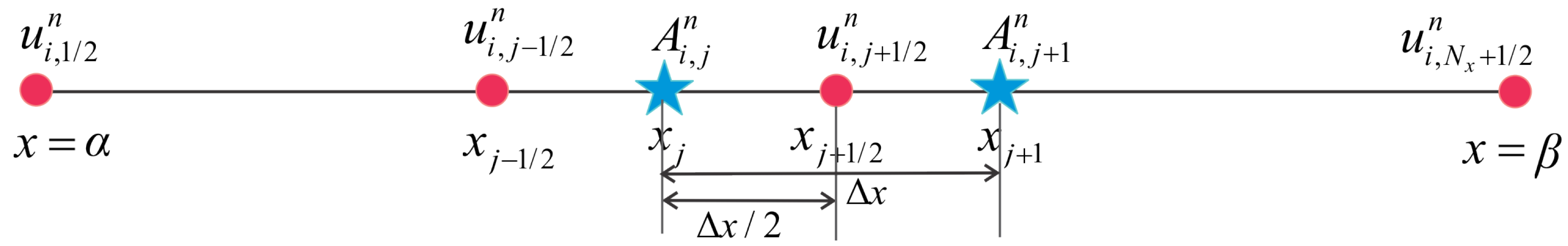
Consider the spatial domain $x\in [\alpha ,\beta ]$ and time domain $t\in [0,T]$ with $\alpha ,\beta ,T\in \mathbb{R}$. The spatial domain is discretized uniformly with a spatial step size $\mathsf{\Delta }x/2$ to yield partition points: $x_{1/2}=\alpha ,x_1,\cdots ,x_{j-1/2},x_j,x_{j+1/2},\cdots ,x_{Nx+1/2}=\beta$, with $N_x={\displaystyle \frac{\beta -\alpha }{\mathsf{\Delta }x}}$. The time domain is also discretized uniformly using the time step $\mathsf{\Delta }t$. In this staggered configuration, we approximate $A_i(x_j,t^n)\equiv A_{i,j}^n$ at full grid points $x_j$. On the other hand, we approximate $u_i(x_{j+1/2},t^n)\equiv u_{i,j+1/2}^n$ at half grid points $x_{j+1/2}$, see Figure 2. The semi discrete equations for (1)–(4) are read as follows.

$$\begin{array}{ccc}& & {\displaystyle \frac{d{A}_{1,j}^n}{dt}}+{\displaystyle \frac{Q_{1,j+1/2}^n-Q_{1,j-1/2}^n}{\mathsf{\Delta }x}}=0,\hfill \\ & & {\displaystyle \frac{d{u}_{1,j+1/2}^n}{dt}}+{\left(u_1{\partial }_x{u}_1\right)}_{j+1/2}^n+g\frac{{\eta }_{1,j+1}^{n+1}-{\eta }_{1,j}^{n+1}}{\mathsf{\Delta }x}=\hfill \end{array}$$

(18)

$$\begin{array}{ccc}& & \nu \frac{u_{1,j+3/2}^n-2u_{1,j+1/2}^n+u_{1,j-1/2}^n}{\mathsf{\Delta }{x}^2},\hfill \end{array}$$

(19)

$$\begin{array}{ccc}& & {\displaystyle \frac{d{A}_{2,j}^n}{dt}}+{\displaystyle \frac{Q_{2,j+1/2}^n-Q_{2,j-1/2}^n}{\mathsf{\Delta }x}}=0,\hfill \\ & & {\displaystyle \frac{d{u}_{2,j+1/2}^n}{dt}}+{\left(u_2{\partial }_x{u}_2\right)}_{j+1/2}^n+gr\frac{{\eta }_{1,j+1}^{n+1}-{\eta }_{1,j}^{n+1}}{\mathsf{\Delta }x}-g^{\prime }\frac{{\eta }_{2,j+1}^{n+1}-{\eta }_{2,j}^{n+1}}{\mathsf{\Delta }x}=\hfill \end{array}$$

(20)

$$\begin{array}{ccc}& & \nu \frac{u_{2,j+3/2}^n-2u_{2,j+1/2}^n+u_{2,j-1/2}^n}{\mathsf{\Delta }{x}^2}.\hfill \end{array}$$

(21)

It should be noted that the numerical damping terms with coefficient $\nu$ have been added to Equations (18) and (21). When the problem being simulated is not fully hyperbolic, as suggested by several authors [1,8,12], these additional damping terms are required to maintain the stability of the numerical scheme. This issue will be discussed in more detail in Section 5.

Returning to (18)–(21), the variables below are computed consistently:

$$\begin{array}{ccc}\hfill A_{i,j}=h_{i,j}{b}_j,& {\eta }_{1,j}=h_{1,j}+h_{2,j}+d_j& {\eta }_{2,j}=h_{2,j}+d_j,Q_{i,j+1/2}={}^{*}{A}_{i,j+1/2}{u}_{i,j+1/2},\hfill \end{array}$$

(22)

where ${}^{*}{A}_{i,j+1/2}$ in (22) is calculated by using the upwind approximation.

$${}^{*}{A}_{i,j+1/2}=\left\{\begin{array}{cc}{A}_{i,j},\hfill & \hfill \mathrm{for}{u}_{i,j+1/2}\ge 0,\\ A_{i,j+1},\hfill & \hfill \mathrm{for}{u}_{i,j+1/2}<0,\end{array}\mathrm{for}i=1,2.\right.$$

(23)

Using the analogy of the momentum conserving approximation of the shallow water equations for one-layer model as described in [10], we use the following approximation for the advection terms:

$$u_i{\partial }_x{u}_i|i,j+1/2={\displaystyle \frac{1}{{\overline{A}}_{i,j+1/2}}}\left({\displaystyle \frac{{\overline{Q}}_{i,j+1}{}^{*}{u}_{i,j+1}-{\overline{Q}}_{i,j}{}^{*}{u}_{i,j}}{\mathsf{\Delta }x}}-u_{i,j+1/2}{\displaystyle \frac{{\overline{Q}}_{i,j+1}-{\overline{Q}}_{i,j}}{\mathsf{\Delta }x}}\right),$$

(24)

whereas

$${\overline{A}}_{i,j+1/2}={\displaystyle \frac{A_{i,j}+A_{i,j+1}}{2}},{\overline{Q}}_{i,j}={\displaystyle \frac{Q_{i,j-1/2}+Q_{i,j+1/2}}{2}},$$

(25)

and the first-order upwind approximation for horizontal velocity is the following.

$${}^{*}{u}_{i,j}=\left\{\begin{array}{cc}\hfill u_{i,j-1/2},& \hfill \mathrm{for}{\overline{Q}}_{i,j}\ge 0,\\ \hfill u_{i,j+1/2},& \hfill \mathrm{for}{\overline{Q}}_{i,j}<0,\end{array}\mathrm{for}i=1,2.\right.$$

(26)

Equations (18)–(21) are semi-discrete schemes. A fully discrete scheme that we used here is obtained by implementing forward time integration to (18)–(21), yielding the following.

$$\begin{array}{ccc}& & A_{1,j}^{n+1}=A_{1,j}^n-\frac{\mathsf{\Delta }t}{\mathsf{\Delta }x}\left[Q_{1,j+1/2}^n-Q_{1,j-1/2}^n\right],\hfill \\ & & u_{1,j+1/2}^{n+1}=u_{1,j+1/2}^n-\mathsf{\Delta }t{\left(u_1{\partial }_x{u}_1\right)}_{j+1/2}^n\hfill \end{array}$$

(27)

$$\begin{array}{ccc}& & -g\frac{\mathsf{\Delta }t}{\mathsf{\Delta }x}\left({\eta }_{1,j+1}^{n+1}-{\eta }_{1,j}^{n+1}\right)+\nu \frac{\mathsf{\Delta }t}{\mathsf{\Delta }{x}^2}\left[u_{1,j+3/2}^n-2u_{1,j+1/2}^n+u_{1,j-1/2}^n\right],\hfill \end{array}$$

(28)

$$\begin{array}{ccc}& & A_{2,j}^{n+1}=A_{2,j}^n-\frac{\mathsf{\Delta }t}{\mathsf{\Delta }x}\left[Q_{2,j+1/2}^n-Q_{2,j-1/2}^n\right],\hfill \\ & & u_{2,j+1/2}^{n+1}=u_{2,j+1/2}^n-\mathsf{\Delta }t{\left(u_2{\partial }_x{u}_2\right)}_{j+1/2}^n-gr\frac{\mathsf{\Delta }t}{\mathsf{\Delta }x}\left({\eta }_{1,j+1}^{n+1}-{\eta }_{1,j}^{n+1}\right)\hfill \end{array}$$

(29)

$$\begin{array}{ccc}& & +g^{\prime }\frac{\mathsf{\Delta }t}{\mathsf{\Delta }x}\left({\eta }_{2,j+1}^{n+1}-{\eta }_{2,j}^{n+1}\right)+\nu \frac{\mathsf{\Delta }t}{\mathsf{\Delta }{x}^2}\left[u_{2,j+3/2}^n-2u_{2,j+1/2}^n+u_{2,j-1/2}^n\right].\hfill \end{array}$$

(30)

Thus, the MCS-schemes for the two-layer shallow water equations are (27)–(30). This scheme is explicit and is based on the leapfrog method, which is discussed in [11] for the case of a one-layer shallow water flow. This staggered grid arrangement has the advantage of being free of numerical damping error. Various test cases will be simulated in Section 4 and Section 5 to validate the proposed scheme. It should be noted that the artificial damping term is only used when the shear stability condition is violated, i.e., when $S>1$.

For the linearized form of the two-layer model (1)–(4), there are two phase speeds: $\sqrt{g{H}_0}$ corresponds to the fast mode, and $\sqrt{g^{\prime }\frac{h_1{h}_2}{H_0}}$ corresponds to the slow mode [18]. Thus, for all simulations performed here, $\mathsf{\Delta }t$ is chosen so that the Courant number is $\sqrt{g{H}_0}\frac{\mathsf{\Delta }t}{\mathsf{\Delta }x}\approx 0.5$. Furthermore, a wet-dry procedure should be used to avoid numerical instability in simulations involving dry areas. In this case, a simple wet-dry procedure is used for each layer; for example, in the lower layer, $u_2$ is calculated by using (30) only when the corresponding cell is wet. While the cell is considered wet if $A_{2,j+1/2}>A_{thres}$, that is, when the wet cross-sectional area exceeds the predetermined value of $A_{thres}$. The same is also holds for the upper layer.

Next, we will first show that the momentum conserving staggered grid scheme admits the well-balanced property. Well balanced here means that the scheme can maintain a steady state; if it was originally steady, it will stay steady. The following discussion is a generalization of the well-balanced property of the one-layer shallow water flow that has been derived in [19].

Theorem 1

(Well balanced semi-discrete). The semi discrete scheme (18)–(20) preserves the steady state at rest: flat surface and interface (${\eta }_1=0$ and ${\eta }_2=0$) and also no motion ($u_1=0$ and $u_2=0$).

Proof. 

Suppose at time $t^n$, the water does not move ($u_{1,j+1/2}^n=0$ and $u_{2,j+1/2}^n=0$), and the water surface and interface are flat (${\eta }_{1,j+1}={\eta }_{1,j}$ and ${\eta }_{2,j+1}={\eta }_{2,j}$). Implementing these on the semi discrete scheme (18)–(20) results in ${\displaystyle \frac{d{A}_{2,j}^n}{dt}}=0$ for $i=1,2$. Furthermore, we have the following.

$$\begin{array}{ccc}& & {\displaystyle \frac{d{A}_{i,j}^n}{dt}}=b_j^{}{\displaystyle \frac{d{h}_{i,j}^n}{dt}}+h_{i,j}^n{\displaystyle \frac{d{b}_j^{}}{dt}}=0,i=1,2.\hfill \end{array}$$

(31)

The above equations can be expressed in terms ${\eta }_1$ and ${\eta }_2$ by using relations (22) to yield the following.

$$\begin{array}{ccc}& & {\displaystyle \frac{d{A}_{2,j}^n}{dt}}\equiv b_j^{}{\displaystyle \frac{d({\eta }_{2,j}+d_j)}{dt}}+({\eta }_{2,j}+d_j){\displaystyle \frac{d{b}_j^{}}{dt}}=0,\hfill \end{array}$$

(32)

$$\begin{array}{ccc}& & {\displaystyle \frac{d{A}_{1,j}^n}{dt}}\equiv b_j^{}{\displaystyle \frac{d({\eta }_{1,j}-{\eta }_{2,j})}{dt}}+({\eta }_{1,j}-{\eta }_{2,j}){\displaystyle \frac{d{b}_j^{}}{dt}}=0.\hfill \end{array}$$

(33)

Since the channel width and depth does not vary in time, after dividing by $b_j^{}\ne 0$, for $j=1,2,\dots ,N_x$, we have ${\displaystyle \frac{d{A}_{2,j}^n}{dt}}={\displaystyle \frac{d{\eta }_{2,j}}{dt}}=0$. Moreover, we also have ${\displaystyle \frac{d{A}_{1,j}^n}{dt}}={\displaystyle \frac{d({\eta }_{1,j}-{\eta }_{2,j})}{dt}}={\displaystyle \frac{d{\eta }_{1,j}}{dt}}=0$. This means that ${\eta }_{1,j}$ and ${\eta }_{2,j}$ are constant at any time $t\ge t^n$.

Furthermore, as ${\eta }_{i,j}$, $i=1,2$ are both flat, Equations (19) and (21) become the following.

$$\begin{array}{ccc}& & {\displaystyle \frac{d{u}_{1,j+1/2}^n}{dt}}\equiv -gr\frac{{\eta }_{1,j+1}^{n+1}-{\eta }_{1,j}^{n+1}}{\mathsf{\Delta }x}=0,\hfill \\ & & {\displaystyle \frac{d{u}_{2,j+1/2}^n}{dt}}\equiv g^{\prime }\frac{{\eta }_{2,j+1}^{n+1}-{\eta }_{2,j}^{n+1}}{\mathsf{\Delta }x}=0,\hfill \end{array}$$

This means that $u_{i,j+1/2}$ is constant at any time $t\ge t^n$. As we know $u_{i,j+1/2}^n=0$, then $u_{i,j+1/2}$ is zero for any $t\ge t_n$. Hence, we have shown that surface and interface stay flat, and the two-fluid system remain motionless at any time $t\ge t_n$; hence, the proof is complete. □

Theorem 2

(Well balanced fully discrete). The fully discrete scheme (27)–(30) preserves the steady state of a lake at rest.

Proof. 

Suppose at time $t^n$, the surface and interface is flat (${\eta }_1=0$ and ${\eta }_2=0$) and does not move ($u_1=0$ and $u_2=0$). Implementing these on (27)–(30) results in the following.

$$A_{i,j}^{n+1}=A_{i,j}^n,fori=1,2.$$

By using (22), the above equations can be expressed in terms ${\eta }_1$ and ${\eta }_2$ as follows.

$$\begin{array}{ccc}& & ({\eta }_{2,j}^{n+1}+d_j)b_j=({\eta }_{2,j}^n+d_j)b_j,\hfill \end{array}$$

(34)

$$\begin{array}{ccc}& & ({\eta }_{1,j}^{n+1}-{\eta }_{2,j}^{n+1})b_j=({\eta }_{1,j}^n-{\eta }_{2,j}^n)b_j.\hfill \end{array}$$

(35)

After being divided by $b_j\ne 0$, Equation (34) becomes ${\eta }_{2,j}^{n+1}={\eta }_{2,j}^n$. Similarly, Equation (35) becomes ${\eta }_{1,j}^{n+1}-{\eta }_{2,j}^{n+1}={\eta }_{1,j}^n-{\eta }_{2,j}^n$ or ${\eta }_{1,j}^{n+1}={\eta }_{1,j}^n$. This means that ${\eta }_i$ is constant for every $t\ge t^n$.

Furthermore, as ${\eta }_{i,j}$ and $i=1,2$ are both flat, Equations (28) and (30) become the following.

$$\begin{array}{ccc}& & u_{1,j+1/2}^{n+1}\equiv -\frac{\mathsf{\Delta }t}{\mathsf{\Delta }x}\left[g\left({\eta }_{1,j+1}^{n+1}-{\eta }_{1,j}^{n+1}\right)\right]=0.\hfill \end{array}$$

(36)

$$\begin{array}{ccc}& & u_{2,j+1/2}^{n+1}\equiv -\frac{\mathsf{\Delta }t}{\mathsf{\Delta }x}\left[gr\left({\eta }_{1,j+1}^{n+1}-{\eta }_{1,j}^{n+1}\right)-g^{\prime }\left({\eta }_{2,j+1}^{n+1}-{\eta }_{2,j}^{n+1}\right)\right]=0\hfill \end{array}$$

(37)

Thus, for any time $t\ge t^n$, we obtain $u_{i,j+1/2}=0$, and ${\eta }_{i,j}$ is constant for $i=1,2$. The proof is complete. □

Steady State of a Lake at Rest

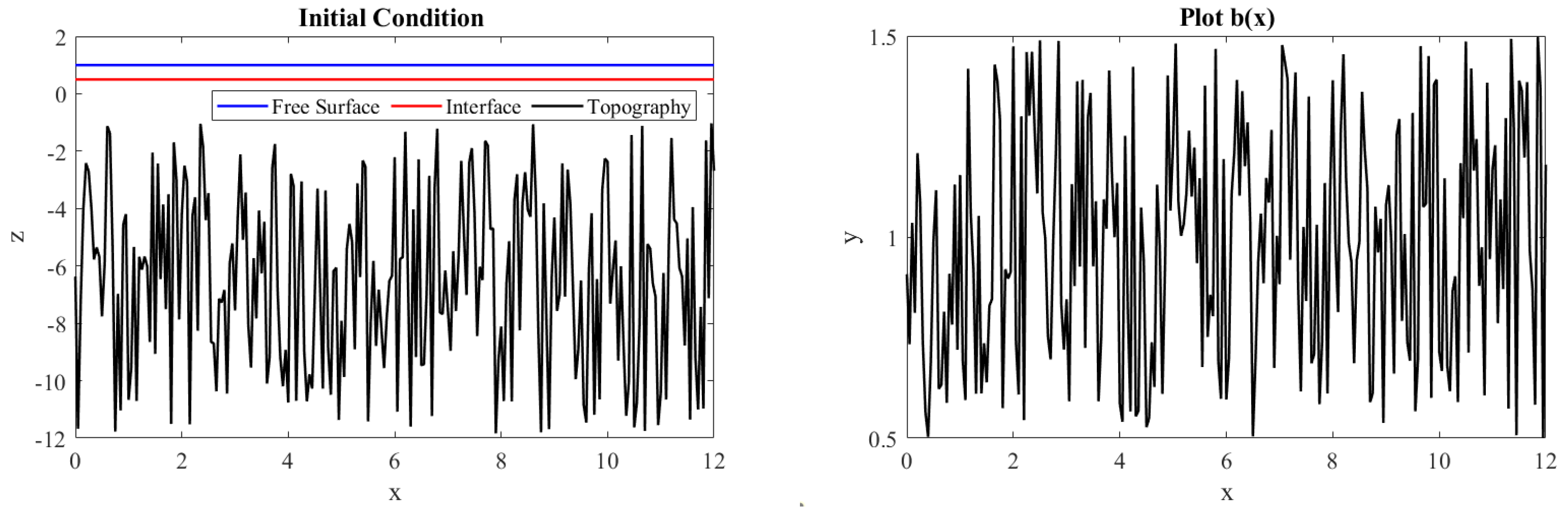
The first test is the simulation of steady state at rest. The spatial domain is $[0,12]$, with the spatial step size $\mathsf{\Delta }x=0.2$. This simulation uses a channel with randomly generated topography $d\left(x\right)$ and width $b\left(x\right)$ as shown in Figure 3. The initial condition is $u_1(x,0)=0$ and $u_2(x,0)=0$ and ${\eta }_1(x,0)=1$ and ${\eta }_2(x,0)=0.5$, which represent flat surface and flat interface at rest. Both left and right boundaries are hard wall boundaries $u_i(0,t)=0$ and $u_i(12,t)=0$ for $i=1,2$.

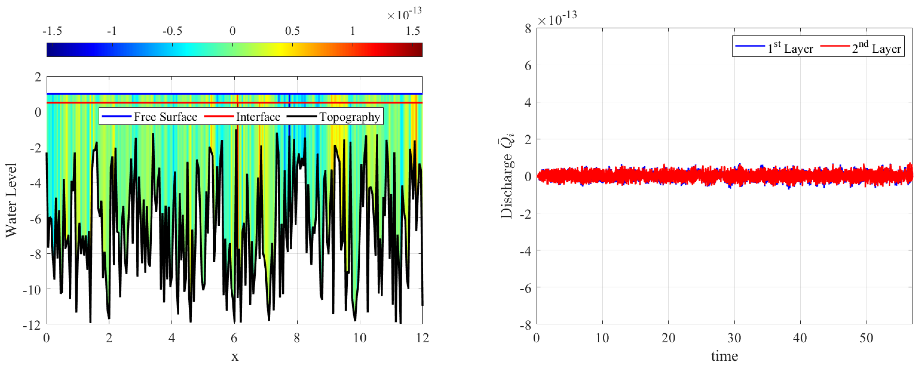
During the calculations it was observed that the free surface and interface remain flat and that velocities $u_1$ and $u_2$ are nearly zero (see Figure 4 (left)). As shown in Figure 4 (right), non-zero discharges $Q_1$ and $Q_2$ appear during computation, but they are still in the order of the round-off error; their values also do not increase over time. This test provides a computational evidence of the well-balanced property of numerical scheme (27)–(30) in the case of a channel with varying bed and width.

4. Simulation of Hyperbolic Case

In this section, we present the results of numerical calculations using the momentum conserving scheme (27)–(30) and simulate the formation of a steady interface in a two-layer flow model under the influence of bottom channel with a sill. All of the test cases presented here are simulated without the use of artificial damping, so we set $\nu =0$; additionally, the problems are hyperbolic with shear parameters less than one.

4.1. Smooth Subcritical Flow

This test case is taken from [7], focusing on simulating a steady interface in a channel with a bottom sill. The computational domain is $x\in [-3,3]$, with a spatial step size of $\mathsf{\Delta }x=0.05$ and gravity acceleration of $g=10$. The channel width is assumed to be one, and the bottom topography consists of a single hump represented by a smooth exponential function.

$$\begin{array}{ccc}& & d\left(x\right)=0.5exp(-x^2)-2.\hfill \end{array}$$

The initial condition is given by $u_i(x,0)=0$, ${\eta }_1(x,0)=0$ and ${\eta }_2(x,0)=-0.5$. The boundary conditions are the discharge $Q_1(-3,t)=0.15$ and $Q_2(-3,t)=-0.15$ at the inflow, and the layer depths are $h_1(3,t)=0.5$ and $h_2(3,t)=1.5$ at the outflow. The steady situation of subcritical flow is depicted in Figure 5 (left). As shown in that figure, the steady interface forms a negative hump, while the free surface remains flat. The lower layer flow moves from left to right ($u_2$ positive), while the upper layer flow moves from right to left ($u_1$ negative). The discharge and energy curves of both layers are depicted in Figure 5 (right); their constant values indicate that the steady state has been reached. We also plot the energy difference and shear instability; the shear instability is less than one, indicating that the problem is still hyperbolic.

4.2. Smooth Transcritical Flow

In this section, we conducted simulations of transcritical flows using the two-layer model. This is the test case presented in [7], also known as the maximal two-layer flow of the rigid-lid model by [4]. To simulate the transcritical flow, we performed two simulations: one where both layers flow in the same direction (parallel flow) and the other where the two layers flow in opposite directions (exchange flow).

Parallel Flow

The computational domain is $x\in [-3,3]$, with spatial step size $\mathsf{\Delta }x=0.05$, and gravity acceleration of $g=10$. The channel width is taken to unity, whereas the bottom topography consists of a single hump represented by a smooth function.

$$d\left(x\right)=\left\{\begin{array}{cc}0.125{\left[cos\left(\pi \frac{x}{2}\right)+1\right]}^2,\hfill & \mathrm{for}-2\le x\le 2,\hfill \\ 0,\hfill & \mathrm{for}\mathrm{otherwise}.\hfill \end{array}\right.$$

(38)

The initial condition used is $u_i(x,0)=0$, ${\eta }_1(x,0)=1.3338331$, and ${\eta }_2(x,0)=1.$

In this case, the fluid in both layers are flowing in the same direction (parallel flow) by adopting the boundary conditions: positive discharges at the left inflow $Q_1(-3,t)=0.09282893$, $Q_2(-3,t)=0.09282893$, and fixed water thicknesses for both layers at the outflow are given by $h_1(3,t)=1.3338331$, where $Q=0.09282893$ and $h_2(3,t)=0.1616669$. Starting from the initial condition, the numerical calculation shows the development of a steady interface, as shown in Figure 6 (left). That steady interface is of transcritical-type, which smoothly connects subcritical flow and supercritical flow on the left and right of the sill, respectively. As shown in that figure, the numerical steady interface agrees well with the analytical steady interface, with a slight deviation on the upstream part of the hump. When a steady state is reached, the discharge curves $Q_1$ and $Q_2$ and the energy curves $E_1$ and $E_2$ show constant values, as shown in Figure 6 (right). These flow parameters must indeed be constant for the steady analytical solution of the rigid-lid model. The fact that our simulation was able to produce a constant value for these parameters indicates that our two-layer MCS scheme can be used to simulate the rigid-lid case. In addition, we observed that the free surface is barely deformed during the simulation of this case. Furthermore, the shear parameter shown in Figure 6 (right) is less than one, indicating that the problem remains hyperbolic.

We also ran another simulation for this smooth transcritical flow in which both layers flow in opposite directions with the same discharge. This is accomplished in the numerical simulation by using the boundary conditions as $Q_1(3,t)=-0.09282893$, $Q_2(-3,t)=0.09282893$, and $h_1(-3,t)=0.4311358$ and $h_2(3,t)=0.1616669$. The numerical simulation yields a steady surface that is similar to the parallel flow case. This is to be expected because, as predicted by the rigid-lid analytic model, the steady interface is determined by the same values of ${\overline{Q}}_r$ and $\mathsf{\Delta }\widehat{E}$ as in the parallel case.

Next, we will discuss the hydraulic aspect of this smooth transcritical steady flow. This description holds for both cases: parallel flow as well as exchange flow, with the discharge ratio ${\overline{Q}}_r=|{\overline{Q}}_1/{\overline{Q}}_2|=1$. The channel topography (38) with constant channel width $\overline{b}=1$ has the form of a smooth hump with a crest $\overline{d}=0.33$ (corresponds to the volume flow rate of $\frac{{\overline{Q}}_2}{{(1-\overline{d})}^{3/2}}=0.21$) and a foot $\overline{d}=0$ (corresponds to the volume flow rate of $\frac{{\overline{Q}}_2}{{(1-\overline{d})}^{3/2}}=0.11$).

On the Froude number plane, we draw two rigid-lid contours: one corresponds to the foot, and another corresponds to the crest of the topographical hump. In numerical simulation, after reaching steady state $\mathsf{\Delta }\widehat{E}=1.5$, we plot the Bernoulli curve with contour $\mathsf{\Delta }\widehat{E}=1.5$. In Figure 7 (right), this Bernoulli curve intersects the rigid-lid contour $=0.11$ at the point A; this condition represents the subcritical upstream part of the steady interface indicated by the point A. Moving forward, at the bottom crest, the Bernoulli and the rigid-lid contour $=0.21$ intersect at B, exactly at a control point with $G^2=1$. Furthermore, the supercritical flow on the downstream part can be recognized by the point C. This downstream condition meets the fact that $h_2$ is small in the downstream area, implying that $F_2^2$ must be large.

4.3. Transcritical Flows with Jump

This is a simulation of steady interface in the case of transcritical flow with jump. Parameters used in this simulation are the same as the previous smooth transcritical case except that here we specify different boundary conditions. Discharges are specified at the inflow $Q_1(-3,t)=Q_2(-3,t)=0.09282893$, and water heights for each layer are specified at the outflow $h_1(3,t)=0.5794783$ and $h_2(3,t)=0.9205217$. The resulting steady interface is depicted in Figure 8; when the flow proceeds over the sill, the subcritical flow accelerates to supercritical, which then undergoes a hydraulic jump to match the boundary condition at the right boundary. The numerical steady interface, as shown in Figure 8 (left), is in good agreement with the exact steady-state solution, and some discrepancy appears at the hydraulic jump location. At the end of the simulation time, the discharge curve in Figure 8 (right) shows a constant value, but the energy curve, especially $E_2$, is not really constant. This indicates that our model is only an approximation of the rigid-lid model. Furthermore, the shear instability curve in Figure 8 (right) is less than one, suggesting that the problem remains hyperbolic.

5. Simulation of Conditionally Hyperbolic Cases

In this second subsection, we simulate steady interface in the case of channel with varying width. We conducted two test cases, both of which turned out to be conditionally hyperbolic case. Thus, in this case, we used a numerical scheme (27)–(30) that includes the artificial damping terms that is three-two orders of magnitude lower than the other terms.

5.1. Maximal Exchange Flows through a Contraction

This test case is known as the maximal exchange flow problem, which was introduced by [1]. On the computational domain $x\in [-1.5,1,5]$, with spatial step size $\mathsf{\Delta }x=0.01$, gravity acceleration $g=9.81$, and damping parameter $\nu =0.002$. This calculation makes use of a flat bed channel with $d\left(x\right)=0$ and varying width given by the following:

$$b\left(x\right)=1+4(1-exp(-{\alpha }^2{x}^2)),$$

(39)

with $\alpha =1.073$. The function (39) represents a normal channel width of $b=5$ with a single contraction $b=1$ at the origin $x=0$ and $b=2$ at $x=\pm 0.5$. Here, we use $h_1(x,0)=0.5$, $h_2(x,0)=0.5$, and $u_1(x,0)=-u_2(x,0)=0.2$ as the initial conditions. In this simulation, the upper layer is flowing to the right, while the lower layer is flowing to the left. The boundary conditions $u_1(-1.5,t)=0.2$ and $u_2(1.5,t)=-0.2$ are used in the numerical simulation, along with absorbing boundaries for the other two, $u_1(1.5,t)$ and $u_2(-1.5,t)$. Note that, for the absorbing boundary, we used the sponge layer technique here by [20]; for the computational interval $-1.5<x<1.5$, we place at the far right $x=1.5$ a sponge layer for $u_1$ on $1.5<x<2$ and at the far left $x=-1.5$ a sponge layer for $u_2$ on $-2<x<-1.5$. When the steady state is reached, the interface forms the maximal exchange flow, as illustrated in Figure 9 (left).

Figure 9 (left) depicts the steady interface and the composite Froude number $G^2$. The numerical steady interface shows a good agreement with the analytical steady interface of the rigid-lid model. We observe that the free surface remains flat during the simulation, indicating that our two-layer numerical scheme can be used to simulate the rigid-lid case. As shown in Figure 9 (right) both the discharges $Q_1$ and $Q_2$ and the energies $E_1$ and $E_2$ are constant, indicating that stability has been achieved. The $G^2$ curve shows that the maximal exchange flow is supercritical on both the upstream and downstream sides of the channel contraction. The control location with $G^2=1$ in this case is the channel contraction $x=0$. In addition, this simulation requires the inclusion of a damping term; otherwise, instability will occur. Indeed, hyperbolicity is not guaranteed in this problem because the shear parameter curve is nearly one throughout the domain, as shown in Figure 9 (right).

In the following, we will recognize the steady interface on the Froude number plane. Following [6] and using (5) and (6), we first rewrite the energy difference formula for the zero channel bed $d=0$ as follows.

$$\begin{array}{ccc}& & \frac{{\widehat{E}}_2-{\widehat{E}}_1}{g^{\prime }{\rho }_2{H}_0}\equiv \mathsf{\Delta }{E}^{\prime }=\frac{1}{2g^{\prime }{H}_0}\left(u_2^2-r{u}_1^2\right)+\frac{h_2}{H_0},\hfill \\ & & \mathsf{\Delta }{E}^{\prime }=\frac{F_2^{-2/3}(1+\frac{1}{2}{F}_2^2)-\frac{1}{2}{\overline{Q}}_r{F}_1^{4/3}}{{\overline{Q}}_r{F}_1^{-2/3}+F_2^{-2/3}}.\hfill \end{array}$$

The later expression is obtained after using (8). The given boundary conditions result in the upper layer flowing to the right, whereas the lower layer flowing to the left at the same rate yields $Q_r=\left|\frac{Q_1}{Q_2}\right|=1$. In this case, the rigid-lid Equation (15) and the Bernoulli equation are read as follows.

$$\begin{array}{ccc}& & F_1^{-2/3}+F_2^{-2/3}={\left(\frac{{\overline{Q}}_2}{\overline{b}}\right)}^{-2/3},\hfill \end{array}$$

(40)

$$\begin{array}{ccc}& & \mathsf{\Delta }{E}^{\prime }=\frac{F_2^{-2/3}(1+\frac{1}{2}{F}_2^2)-\frac{1}{2}{F}_1^{4/3}}{F_1^{-2/3}+F_2^{-2/3}}.\hfill \end{array}$$

(41)

Our interest is on the maximal two-way exchange flow between two infinite reservoirs; with density ${\rho }_1$ on the left and ${\rho }_2$ on the right. In this case, the inflowing layer spreads out to the point where the fluid thickness approaches zero. Since $Q_i$ is finite, the vanishing $h_i$ implies a Froude number $F_i$ that tends to infinity for $i=1,2$. The point A in Figure 10 (left) represents a position near reservoir ${\rho }_1$, with $F_2\to \infty$, whereas the point C represents a position near reservoir ${\rho }_2$, with $F_1\to \infty$. Consider Figure 10 (right), among several Bernoulli curves, there is only one level curve, i.e., with $\mathsf{\Delta }{E}^{\prime }=0.5$ that satisfies these boundary conditions; that curve is plotted as a thick solid curve. This Bernoulli curve intersects the criticality condition (9) at a point $(F_1^2=\frac{1}{2},F_2^2=\frac{1}{2})$, i.e., the point B, located at the narrowest section, which becomes a control with $G^2=1$. Furthermore, the rigid-lid curve (40) with contour $\frac{{\overline{Q}}_2}{\overline{b}}=\frac{1}{4}$ passes through the point B. Thus, the solid curve $A-B-C$ in the Froude number plane represents the steady interface of the maximal exchange flow. Moreover, this steady flow is supercritical on both sides of the control.

5.2. Exchange Flows through Sill and Contraction

The final test case is taken from [1]. The steady interface in this case represents the exchange flow through a channel with contraction and a bottom sill. The computational domain is $x\in [-1,2]$ with the spatial step size $\mathsf{\Delta }x=0.01$ and gravitational acceleration of $g=9.81$, and the damping parameter is $\nu =0.01$. The channel beds and widths are given by the following:

$$\begin{array}{ccc}& & d\left(x\right)={sech}^2\left(\beta x\right),andb\left(x\right)=0.5+1.5(1-exp(-{\alpha }^2{(x-1)}^2)),\hfill \end{array}$$

where $\alpha =0.673$ for $x\le 1$, $\alpha =1.273$ for $x\ge 1$, and $\beta =3.75$.

For this simulation, the initial conditions are $h_1(x,0)=1$, $h_2(x,0)=1$, $u_1(x,0)=0.2$, and $u_2(x,0)=-0.18$. To achieve an exchange flow with the upper layer flowing to the right and the lower layer flowing to the left, we use boundary conditions $u_1(-1,t)=0.2$ and $u_2(2,t)=-0.18$, with absorbing boundary conditions for the upper layer downstream and the lower layer upstream. In this case, the absorbing boundary is built using sponge layer technique similar to those described in Section 5.1.

Figure 11 (left) depicts the steady interface and the composite Froude number $G^2$. The numerical steady interface shows a good agreement with the analytical steady interface of the rigid-lid model. We observe that the free surface remains flat during the simulation, indicating that our two-layer numerical scheme can be used to simulate the rigid-lid case. Figure 11 (right) shows that both the discharges $Q_1$ and $Q_2$, as well as the energies $E_1$ and $E_2$, are constant, indicating that steady state has been achieved. The $G^2$ curve shows that the maximal exchange flow is supercritical on both the upstream and downstream sides of the channel, with a subcritical area trapped between the two controls, i.e., at the bottom sill $x=0$ and at the channel contraction $x=1$. The shear parameter curve shown in Figure 11 (right) is greater than one on the upstream side of the sill, therefore, hyperbolicity is not guaranteed for this problem. To avoid numerical instability, the numerical damping term must be incorporated

6. Conclusions

We have proposed an extension of the momentum conserving staggered-grid scheme (MCS) for the two-layer shallow water flows in channels with varying bed and width. Formulation of the scheme is a direct analog of the MCS scheme for the one-layer shallow water equations. The scheme is explicit and well-balanced, and it has been tested with the steady-at-rest case. The scheme was validated using various test cases of steady interface in a channel with bottom sill, including subcritical flow, smooth transcritical flow, and transcritical flow with hydraulic jump. The obtained results agree well with the exact steady interface of the two-layer rigid-lid model. In the simulation of the maximal exchange flow, the numerical scheme succeeded in producing a steady interface. In this simulation, an artificial numerical damping was used to avoid numerical instability. This was necessary because the problem is classified as conditionally hyperbolic. We concluded that the MCS scheme performs well in simulating various steady flows in channels with varying bed and width. However, the scheme developed here is limited to rectangular cross-section channels.

References

1. Helfrich, K.R. Time Dependant Two Layer Hydraulic Exchange Flows. J. Phys. Oceanogr. 1995, 25, 359–372. [Google Scholar] [CrossRef] [Green Version]
2. Brandt, P.; Alpers, W.; Backhaus, J.O. Study of the generation and propagation of internal waves in the Strait of Gibraltar using a numerical model and synthetic aperture radar images of the European ERS 1 satellite. J. Geophys. Res. C Ocean. 1996, 101, 14237–14252. [Google Scholar] [CrossRef]
3. Castro, M.J.; García-Rodríguez, J.A.; González-Vida, J.M.; Marías, J.; Parés, C.; Vázquez-Cendón, M.E. Numerical simulation of two-layer shallow water flows through channels with irregular geometry. J. Comput. Phys. 2004, 195, 202–235. [Google Scholar] [CrossRef]
4. Farmer, D.M.; Armi, L. Maximal two-layer exchange over a sill and through the combination of a sill and contraction with barotropic flow. J. Fluid Mech. 1986, 164, 53–76. [Google Scholar] [CrossRef]
5. Brandt, P.; Rubino, A.; Alpers, W.; Backhaus, J.O. Internal waves in the Strait of Messina studied by a numerical model and synthetic aperture radar images from the ERS 1/2 satellites. J. Phys. Oceanogr. 1997, 27, 648–663. [Google Scholar] [CrossRef] [Green Version]
6. Armi, L. The hydraulics of two flowing layers with different densities. J. Fluid Mech. 1986, 163, 27–58. [Google Scholar] [CrossRef] [Green Version]
7. Abgrall, R.; Karni, S. Two-layer shallow water system: A relaxation approach. SIAM J. Sci. Comput. 2009, 31, 1603–1627. [Google Scholar] [CrossRef]
8. Li, S.S.; Lawrence, G.A. Unsteady two-layer hydraulic exchange flows with friction. J. Fluid Mech. 2009, 633, 99–114. [Google Scholar] [CrossRef]
9. Castro-Díaz, M.J.; Fernández-Nieto, E.D.; González-Vida, J.M.; Parés-Madroñal, C. Numerical treatment of the loss of hyperbolicity of the two-layer shallow-water system. J. Sci. Comput. 2011, 48, 16–40. [Google Scholar] [CrossRef] [Green Version]
10. Swastika, P.V.; Pudjaprasetya, S.R.; Wiryanto, L.H.; Hadiarti, R.N. A momentum-conserving scheme for flow simulation in 1D channel with obstacle and contraction. Fluids 2021, 6, 26. [Google Scholar] [CrossRef]
11. Pudjaprasetya, S.R.; Magdalena, I. Momentum Conservative Schemes for Shallow Water Flows. East Asian J. Appl. Math. 2014, 4, 152–165. [Google Scholar] [CrossRef]
12. Frankcombe, L.M.; Hogg, A.M.C. Tidal modulation of two-layer hydraulic exchange flows. Ocean Sci. 2007, 3, 179–188. [Google Scholar] [CrossRef] [Green Version]
13. Lane-Serff, G.F.; Smeed, D.A.; Postlethwaite, C.R. Multi-layer hydraulic exchange flows. J. Fluid Mech. 2000, 416, 269–296. [Google Scholar] [CrossRef]
14. Kurganov, A.; Petrova, G. Central-upwind schemes for two-layer shallow water equations. SIAM J. Sci. Comput. 2009, 31, 1742–1773. [Google Scholar] [CrossRef] [Green Version]
15. Stelling, G.S.; Duinmeijer, S.P.A. A staggered conservative scheme for every Froude number in rapidly varied shallow water flows. Int. J. Numer. Methods Fluids 2003, 43, 1329–1354. [Google Scholar] [CrossRef]
16. Erwina, N.; Adytia, D.; Pudjaprasetya, S.R.; Nuryaman, T. Staggered Conservative Scheme for 2-Dimensional Shallow Water Flows. Fluids 2020, 5, 149. [Google Scholar] [CrossRef]
17. Pudjaprasetya, S.R.; Risriani, V.M.; Iryanto. Numerical simulation of propagation and run-up of long waves in U-shaped bays. Fluids 2021, 6, 146. [Google Scholar] [CrossRef]
18. Pudjaprasetya, S.R.; Magdalena, I. Two-Layer Non-Hydrostatic Model for Generation and Propagation of Interfacial Waves. China Ocean Eng. 2019, 33, 65–72. [Google Scholar] [CrossRef]
19. Mungkasi, S.; Magdalena, I.; Pudjaprasetya, S.R.; Wiryanto, L.H.; Roberts, S.G. A staggered method for the shallow water equations involving varying channel width and topography. Int. J. Multiscale Comput. Eng. 2018, 16, 231–244. [Google Scholar] [CrossRef]
20. Stelling, G.; Zijlema, M. An accurate and efficient finite-difference algorithm for non-hydrostatic free-surface flow with application to wave propagation. Int. J. Numer. Methods Fluids 2003, 23, 1–23. [Google Scholar] [CrossRef]
Figure 1. Sketch of the problem and notations. (Left) side view; (right) top view.
Fluids 06 00346 g001
Figure 2. Sketch of the computational domain α x β with the staggered grid partition and locations of the computed variables A i , j n and u i , j + 1 / 2 n , for i = 1 , 2 .
Fluids 06 00346 g002
Figure 3. (Left) The randomly generated channel bed and the initial free surface and interface. (Right) The randomly generated channel width.
Fluids 06 00346 g003
Figure 4. Snapshot of simulation results which show (left) flat surface and interface, with zero velocities (indicated by the color scale) and (right) nearly zero discharges.
Fluids 06 00346 g004
Figure 5. (Left) Steady interface in the case of subcritical flow. The fluid velocity for each layer is represented by the color scale. (Right) Plots of discharge and energy for each layer, as well as the shear parameter.
Fluids 06 00346 g005
Figure 6. (Left) Steady interface in the case of smooth transcritical flow, where both fluid layers flowing in the same direction. The fluid velocity for each layer is represented by the color scale. (Right) Plots of discharge and energy for each layer, as well as the shear parameter.
Fluids 06 00346 g006
Figure 7. (Left) Side view of the steady interface of the smooth transcritical flow due to a bottom sill (not to scale). (Right) The Froude number planes with several contours of the rigid-lid and Bernoulli are plotted in red and blue labels, respectively, whereas the straight line represents the criticality condition (9). The Bernoulli contour, shown as a thick solid curve A B C , depicts the steady interface of the smooth transcritical flow.
Fluids 06 00346 g007
Figure 8. (Left) Steady interface in the case of transcritical flow with jump, where both fluid layers flowing in the same direction. The fluid velocity for each layer is represented by the color scale. (Right) Plots of discharge and energy for each layer, as well as the shear parameter.
Fluids 06 00346 g008
Figure 9. (Left) Steady interface in the case of maximal two layer exchange flow. The fluid velocity for each layer is represented by the color scale. (Right) Plots of discharge and energy for each layer, as well as a shear parameter with a value of one, indicating a conditional hyperbolicity based on (10).
Fluids 06 00346 g009
Figure 10. (Left) Top and side views of the steady interface of the maximal exchange flow due to contraction (not to scale). (Right) The Froude number planes with several contours of the rigid-lid and Bernoulli are plotted in red and blue labels, respectively, whereas the straight line represents the criticality condition (9). The Bernoulli contour, shown as a solid curve A B C , depicts the steady interface of the maximal exchange flow.
Fluids 06 00346 g010
Figure 11. (Left) Steady interface in the exchange flow through channel with contraction and a bottom sill. (Right) Plots of discharge and energy for each layer; the shear parameter (10) is greater than one, indicating a loss of hyperbolicity in that region.
Fluids 06 00346 g011
Publisher’s Note: MDPI stays neutral with regard to jurisdictional claims in published maps and institutional affiliations.